Music Similarity Detection Through Comparative Imagery Data

Abstract

In music, plagiarism has been an important but troubled issue, which becomes ever more critical with the widespread usage of generative AI tools. Meanwhile, the development of techniques for music similarity detection has been hampered by the scarcity of legally verified data on plagiarism. In this paper, we present a technical solution for training music similarity detection models through the use of comparative imagery data. With the aid of feature-based analysis and data visualization, we conducted experiments to analyze how different music features may contribute to the judgment of plagiarism. While the feature-based analysis guided us to focus on a subset of features, whose similarity is typically associated with music plagiarism, data visualization inspired us to train machine learning models using such comparative imagery instead of using audio signals directly. We trained feature-based sub-models (convolutional neural networks) using imagery data and an ensemble model with Bayesian interpretation for combining the predictions of the sub-models. We tested the trained model with legally verified data as well as AI-generated music, confirming that the models produced with our approach can detect similarity patterns which are typically associated with music plagiarism. Furthermore, using imagery data as the input and output of an ML model has been proven to facilitate explainable AI.

1. Introduction

It is common for artists to be influenced by the greats of their time, and imitate their work and style in their early years. After all, as Oscar Wilde said, “imitation is the sincerest form of flattery” [1]. However, when imitation is of a certain form or reaches a certain level, it may become copyright infringement and plagiarism. In recent years, music generated by generative artificial intelligence (AI) models gained much attention, with a swirl of excitement, suspicion, and fear. There are ongoing efforts to develop a copyright and AI framework that rewards human creativity (e.g., [2]).

Existing technical methods for detecting similarity patterns in music can broadly be categorized into two groups: context-based and content-based. Context-based methods use contextual metadata, an umbrella term for musical information such as user ratings, radio and user playlists that the songs are a part of, and the lyrics and collaborative tags made by users on music websites [3]. Meanwhile, content-based methods extract music features from audio files, such as melodic structure, among many others.

Contextual methods perform well in music recommendation systems and music clustering based on similarity. For example, Schedl et al. [4] investigated the similarity between a wide array of artist’s music and developed a recommendation strategy using text-based metadata. Karydis et al. [5] compared user-assigned tags and features extracted from audio signal and showed that the former was outperformed by the latter in classifying the genre of musical pieces. Spärck Jones [6] proposed a weighting system for moderating the association between tags and songs in retrieval, which was utilized in the term frequency-inverse document frequency (TFIDF) metric. According to Beel et al. [7], 83% of text-based recommendation systems currently implement TFIDF.

Content-based methods exploit stored music pieces (audio or MIDI) in various ways, using text-based and audio-based approaches. Text-based approaches focus on textual representations where each music piece is an array of symbols encoding the relative locations of musical notes chronologically. With textual representations, some researchers have applied commonly used similarity metrics, such as cosine similarity or Euclidean distance, in the literature (e.g., [8,9]). Others developed their own music similarity metrics, e.g., fuzzy vectorial-based similarity [9]. Text-based methods have been used to detect melodic plagiarism. However, an unsettled question is whether melodic similarity is the only factor of music plagiarism.

Audio-based approaches rely on features extracted from music files and analyze music pieces in their feature vectors. Typically, music signals contained in audio files are processed via variations of Fourier and wavelet transforms. Li and Ogihara [10] used spectral features to find similar songs and detect emotion in music. Nguyen et al. [11] used melodies extracted from MIDI files to cluster similar songs, in conjunction with the K-nearest neighbors (kNN) and support vector machine (SVM) methods. In essence, this is similar to a text-based approach. Nair [12] evaluated the performance of several machine learning (ML) techniques for detecting music plagiarism, including logistic regression, naive Bayes, and random forest, among others. Karydis et al. [5] applied neural networks to spectral features. As there are numerous ways for specifying a feature in music, many features, which may be known or unknown currently, may potentially be used to characterize music plagiarism. It will be a long-term endeavor for researchers to find the most effective feature specifications (in a vast feature space) for detecting music plagiarism.

While there is a need to improve the legal definition as to how musical plagiarism is defined for a specific type and level of musical similarity, it is desirable for us to make technical progress that can provide analytical tools to assist in legal processes. While there is little doubt that we need to develop advanced AI technology for detecting music plagiarism, it is necessary for us to address a number of technical challenges, including the following:

C1.

As mentioned above, apart from melodic features, there is a vast feature space for us to explore in order to identify other features or combinations of features that can help detect music plagiarism.

C2.

There is an insufficient amount of legally verified data on music plagiarism for training ML models to detect music plagiarism or to identify or formulate useful feature specifications in detecting music plagiarism.

C3.

Music plagiarism is a serious allegation, and any ML model designed for suggesting such an allegation has to be treated with caution. How to interpret and explain ML predictions is a generally challenging topic commonly referred to as explainable AI.

In this paper, we present a study on developing ML models to detect music similarity patterns. We addressed the first challenge, C1, by analyzing and visualizing different features in terms of their similarity and dissimilarity in a number of known cases where the level of music similarity is relatively certain. This allowed us to focus our data collection and model development efforts on these indicative features. Meanwhile, we developed different sub-models for different features and trained an ensemble model to integrate these sub-models to make decisions collectively, avoiding over-reliance on a single feature.

To address the second challenge, C2, we created a dataset for the training and validation of ML models, while keeping the data of known cases for independent testing outside the development workflow. Inspired by feature-based analysis and visualization in addressing C1, we proposed a novel method for training ML models to detecting music similarity based on comparative imagery. Information-theoretical analysis indicates that the space of such comparative imagery has much lower entropy than the space of the original music signal data for creating the imagery, suggesting that training ML models requires less data in the former than the latter.

Data visualization has played an indispensable role in explainable AI, the comparative imagery used for testing an ML model provided an effective means for humans to scrutinize and interpret the judgment of the ML model, hence enhancing the explainability of the ML model. In particular, when we applied the trained ML model to a collection of AI-generated music, we were often not sure about the correctness of the similarity patterns detected by the model. By visualizing the comparative images for individual features, we were able to reason how the model made its decision.

In summary, the contributions of this work include the following:

• A broad analysis of the relationship between music feature similarity and music similarity in the context of copyright infringement and plagiarism [addressing C1].
• A novel method for using comparative imagery as intermediate data to train ML models to detect music similarity, while improving the interpretability of model predictions [addressing C2 and C3].
• An ensemble approach to develop an ML model for music similarity detection, which enables a long-term modular approach for results analysis, performance monitoring, and improvement of sub-models [addressing C2].
• A set of experiments where the ensemble model is applied to different testing data, including independent data differing significantly from the training data, known plagiarism data, and a collection of AI-generated music, demonstrating the feasibility and merits of the proposed method [addressing C1, C2, and C3].

In the remainder of this paper, we first describe the technical methods used in different parts of this work in Section 2. This is followed by Section 3, where we report the analytical results of different features in terms of their potential relevance to music plagiarism, and Section 4, where we report our development of ML models and our experimental results. In Section 5, we provide our concluding remarks and suggestions for future work.

2. Methods

In this section, we first describe the theoretical reasoning behind our approach, then present the four main methods used in this work, and finally outline our system architecture for enabling the development of machine learning (ML) models for music similarity detection and the deployment of these models in an ensemble manner.

2.1. Information-Theoretical Reasoning

In information theory, a function or a process is referred to as a transformation, which we denote as P here. The set of all possible data that P can receive is referred to as an input alphabet and the set of all possible data that P can produce is an output alphabet. As illustrated in Figure 1a, the two alphabets are denoted as ${\mathbb{Z}}_{\mathit{in}}$ and ${\mathbb{Z}}_{\mathit{out}}$, respectively. When a machine learning (ML) model is used to determine whether two pieces of music are similar, P is the model, ${\mathbb{Z}}_{\mathit{in}}$ consists of all possible pairs of music to be compared, and ${\mathbb{Z}}_{\mathit{out}}$ consists of all possible decisions that the model may produce. Typically, a model may return a similarity judgment in two or a few levels. Hence, the entropy of the output alphabet, $\mathcal{H}\left({\mathbb{Z}}_{\mathit{out}}\right)$, is no more than 3 bits for eight or fewer levels. Meanwhile, the informative space for all possible pairs of music is huge, and the entropy of the input alphabet, $\mathcal{H}\left({\mathbb{Z}}_{\mathit{in}}\right)$, is very high. Hence, $\mathcal{H}\left({\mathbb{Z}}_{\mathit{in}}\right)\gg \mathcal{H}\left({\mathbb{Z}}_{\mathit{out}}\right)$ and the model incurs a huge entropy loss. As Chen and Golan observed, such entropy loss is ubiquitous in most (if not all) decision workflows [13]. If the entropy reduction (measured as alphabet compression) is too much and too fast by an unreliable transformation, decision errors are more likely (measured as potential distortion) [13].

In practice, a common approach to address the high level of decision errors is to decompose a complex transformation P into a series of less complex transformations, $P_1,P_2,\dots ,P_n$, where entropy is reduced gradually as illustrated in Figure 1b. For some intermediate transformations, humans can inject more knowledge in developing better algorithms, models, software, etc. For some intermediate alphabets, humans can visualize and interpret intermediate data, gaining confidence about the workflow. In essence, explainable AI is facilitated by such workflow decomposition.

Figure 1a can also represent an ML workflow, where ${\mathbb{Z}}_{\mathit{out}}$ consists of all possible models that may be learned using the training and testing process P. The initial search space for the optimal model in ${\mathbb{Z}}_{\mathit{out}}$ is huge (i.e., it has very high initial entropy), but the process P uses the input data (or its statistics) as constraints to narrow down the search space iteratively, and in effect, change its probability of each model in the space so as to be found as the optimal model. The change in the probabilities in the search space reduces the entropy of ${\mathbb{Z}}_{\mathit{out}}$. When the input data are scarce, P does not have reliable statistics or invoke a sufficient number of iterations to change the probability of each model in the space appropriately, resulting in an unreliable model being found at the end of the process.

As discussed in Section 1, for music similarity detection, data scarcity is a major challenge. Therefore, instead of training a complex model that detects similarity directly from music signals, we adopted the common approach to reduce entropy gradually by decomposing both the model development and model deployment workflows as shown in Figure 1c. For example, transforming music pieces into fixed-length segments facilitates entropy reduction for both new music and known music, i.e.,

$$\mathcal{H}\left({\mathbb{Z}}_{\mathit{nm}}\right)>\mathcal{H}\left({\mathbb{Z}}_{\mathit{ns}}\right)\mathrm{and}\mathcal{H}\left({\mathbb{Z}}_{\mathit{km}}\right)>\mathcal{H}\left({\mathbb{Z}}_{\mathit{ks}}\right).$$

Meanwhile, human knowledge can help address data scarcity in ML workflows [14]. Tam et al. [15] estimated the amount of extra information provided by ML developers in two case studies. In this work, we make use of feature extraction algorithms as a form of human knowledge, and these algorithms are essentially transformations facilitating entropy reduction from inputs to outputs. We also employ similarity visualization to enable the involvement of humans in interpreting the predictions made by ML models. This is a way of using human knowledge to reduce uncertainty during model development as well as deployment. In the following four subsections, we will describe four methods used in the workflow as shown in Figure 1c to show how they facilitate entropy reduction further.

2.2. Method 1: Feature-Based Analysis

Feature-based analysis has been widely used in signal processing in general and music analysis in particular. Transforming signal representations of music segments to their feature representations facilitates entropy reduction, and in the context of Figure 1c, we have

$$\mathcal{H}\left({\mathbb{Z}}_{\mathit{ns}}\right)>\mathcal{H}\left({\mathbb{Z}}_{\mathit{nf}}\right)\mathrm{and}\mathcal{H}\left({\mathbb{Z}}_{\mathit{ks}}\right)>\mathcal{H}\left({\mathbb{Z}}_{\mathit{kf}}\right).$$

There are numerous feature specifications for music in the literature. Many specifications have different variants controlled by parameters. It is not difficult to anticipate that some features are more relevant to music similarity detection than others. For example, one may reasonably assume that similarity detection should not influenced by a feature representing the loudness of the notes or a feature indicating the instrument used in playing a musical piece. Nevertheless, for many features, there is no previous report about whether they are relevant to music similarity detection.

Therefore, it is necessary to conduct experiments to discover such relevance. For the experimentation in this work, we selected a total of 33 features, including 7 melodic features, 8 pitch statistics features, 7 chord and vertical interval features, 7 rhythm- and beat-related features, and 4 texture features. The descriptions of these features are given in

Table 1. The set of melodic features initially selected for experimentation [16].

Feature	Definition
Melodic Interval Histogram	A histogram with bins representing different melodic intervals expressed in semitones where the magnitudes of each bin shows the amount of times a melody consisting of that interval was played. The bin indices show how many semitones are in that melodic interval.
Amount of Arpeggiation	Fraction of melodic intervals that are repeated notes, minor thirds, major thirds, perfect fifths, minor sevenths, major sevenths, octaves, minor tenths or major tenths.
Melodic Pitch Variety	Average number of notes that are produced in a MIDI channel before a note’s pitch is repeated.
Number of Common Melodic Intervals	Number of different melodic intervals that each account individually for at least 9% of all melodic intervals.
Mean Melodic Interval	Mean average (in semitones) of the intervals involved in each of the melodic intervals in the piece.
Direction of Melodic Motion	Fraction of melodic intervals that are rising in pitch.
Distance Between Most Prevalent Melodic Intervals	Absolute value of the difference (in semitones) between the most common and second most common melodic intervals in the piece.

,

Table 2. The set of pitch statistics features initially selected for experimentation [16].

Feature	Definition
Pitch Class Histogram	A histogram with bins representing each pitch class where the magnitudes of each bin shows the amount of times a note from that class was played. The harmonics of each pitch class are grouped together.
Folded Fifths Pitch Class Histogram	A histogram derived directly from the pitch class histogram with the bins ordered by perfect fifth interval separation instead of semitones.
Strong Tonal Centers	Number of isolated peaks in the fifths pitch histogram that each individually account for at least 9% of all notes in the piece.
Number of Common Pitch Classes	Number of pitch classes that account individually for at least 20% of all notes.
Mean Pitch Class	Mean pitch class value, averaged across all pitched notes in the piece. A value of 0 corresponds to a mean pitch class of C, and pitches increase chromatically by semitone in integer units from there.
Pitch Class Variability	Standard deviation of the pitch classes of all pitched notes in the piece. Provides a measure of how close the pitch classes as a whole are to the mean pitch class.
Pitch Class Skewness	Skewness of the pitch classes of all pitched notes in the piece.
Pitch Class Kurtosis	Kurtosis of the pitch classes of all pitched notes in the piece. Provides a measure of how peaked or flat the pitch class distribution is.

,

Table 3. The set of chord and vertical interval features initially selected for experimentation [16].

Feature	Definition
Wrapped Vertical Interval Histogram	A vertical interval histogram wrapped by an octave (there are 12 bins) with each bin corresponding to a different vertical interval expressed in semitones where the magnitudes represent the amount of times that vertical interval was played.
Chord-Type Histogram	A normalized histogram with each bin corresponds to a chord type where the magnitudes represent the amount of times that chord was played.
Most Common Vertical Interval	The interval in semitones corresponding to the wrapped vertical interval histogram bin with the highest magnitude.
Variability of Number of Simultaneous Pitch Classes	Standard deviation of the number of different pitch classes sounding simultaneously.
Second Most Common Vertical Interval	The interval in semitones corresponding to the wrapped vertical interval histogram bin with the second highest magnitude.
Distance Between Two Most Common Intervals	The interval in semitones between the wrapped vertical interval histogram bins with the two most common vertical intervals.
Chord Duration	Average duration of a chord in units of time corresponding to the duration of an idealized quarter note.

,

Table 4. The set of rhythm- and beat-related features initially selected for experimentation [16].

Feature	Definition
Rhythmic Value Histogram	A normalized histogram where the value of each bin specifies the fraction of all notes in the piece with a quantized rhythmic value corresponding to that of the given bin.
Beat Histogram	A normalized histogram where the value of each bin specifies the beats per minute, where the magnitudes of each bin represent the relative frequency of that beat in the musical piece.
Rhythmic Value Median Run Lengths Histogram	A normalized feature vector that indicates, for each rhythmic value, the normalized median number of times that notes with that rhythmic value occur consecutively (either vertically or horizontally) in the same voice (MIDI channel and track).
Rhythmic Value Variability	Standard deviation of the note durations in quarter notes of all notes in the music. Provides a measure of how close the rhythmic values are to the mean rhythmic value.
Prevalence of Most Common Rhythmic Value	The fraction of all notes that have a rhythmic value corresponding to the most common rhythmic value in the music.
Number of Strong Rhythmic Pulses	Number of tempo-standardized beat histogram peaks with normalized magnitudes over 0.1.
Polyrhythms	Number of tempo-standardized beat histogram peaks with magnitudes at least 30% as high as the magnitude of the highest peak, and whose bin labels are not integer multiples of the bin label of the peak with the highest magnitude.

and

Table 5. The set of texture features initially selected for experimentation [16].

Feature	Definition
Parallel Motion	Fraction of movements between voices that consist of parallel motion.
Similar Motion	Fraction of movements between voices that consist of similar motion.
Contrary Motion	Fraction of movements between voices that consist of contrary motion.
Oblique Motion	Fraction of movements between voices that consist of oblique motion.

. They were implemented using the jSymbolic 2.2 API. In Section 3, we present and analyze the results of our experimentation on these features.

2.3. Method 2: Similarity Visualization

Data visualization has been used in text similarity detection (e.g., [17]) as well as in developing ML models for music applications (e.g., [18]). Data visualization played three roles in this work. Firstly, visualization allowed us to observe how much a feature may be relevant to music similarity detection and prioritize computational resources for harvesting training and testing data for developing ML models. In Section 3, we present and analyze the results of our experimentation on features with the aid of such visualization.

Secondly, the comparative imagery used to depict feature similarity was used for training and testing ML models. We will describe this in detail in the next subsection.

Thirdly, whenever an ML model or an ensemble decision process produced a decision, we found it useful to use visualization to help interpret the decision. In some cases, visualization helped us to identify possible causes of erroneous decisions, and in many cases, visualization enabled us to explain why the decision was reached, gaining confidence about the validity of the workflow.

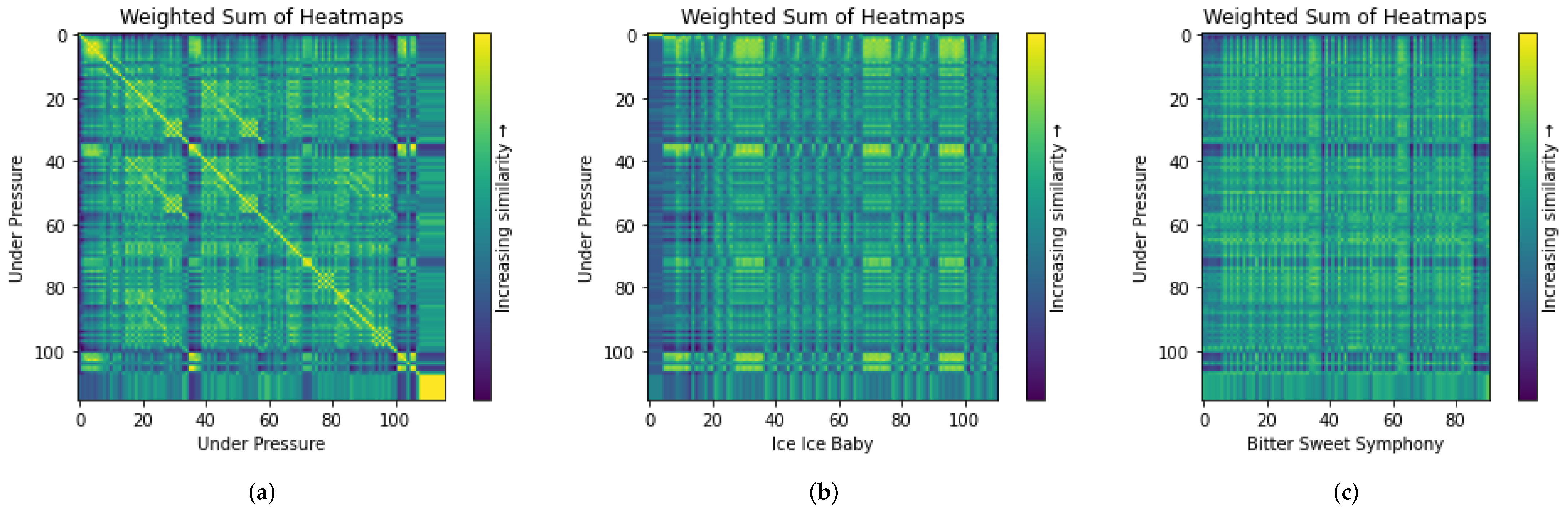
Figure 2 shows three heatmap visualizations, where the x and y axes correspond to the temporal sequences of two songs, respectively. In this work, we compare two music pieces in the unit of a bar. The three songs have 116 (Under Pressure), 113 (Ice Ice Baby), and 91 (Bitter Sweet Symphony) bars, respectively. The color of each cell indicates the level of similarity between the x-th bar of one song and the y-th bar of the other. The computed similarity level is in the range of [0, 1], and it is encoded using a continuous colormap, with a bright yellow color (RGB: 253, 231, 37) for 1 and dark purple (RGB: 68, 1, 84) for 0. The in-between colors are linearly interpolated. As shown in the legend on the right, bright yellow or green colors indicate high similarity while dark purple or blue indicate dissimilarity. In Figure 2a, we can easily observe the strong self-similarity along the diagonal line when the song “Under Pressure ⯈” by Queen and David Bowie (https://github.com/asaner7/imagery-music-similarity/blob/main/songs-in-paper/UnderPressure_mp3.mp3, accessed on 30 May 2025) is compared with itself. Meanwhile, we can also observe smaller similarity patterns in other temporal regions.

In Figure 2b, “Under Pressure” is compared with “Ice Ice Baby ⯈” by Vanilla Ice (https://github.com/asaner7/imagery-music-similarity/blob/main/songs-in-paper/IceIceBaby_mp3.mp3, accessed on 30 May 2025). “Ice Ice Baby” is part of a well-documented plagiarism lawsuit, the verdict of which confirmed that Vanilla Ice had copied the guitar riff of “Under Pressure” in his song. From the heatmap visualization, we can observe patterns of similarity in some temporal regions as well as dissimilarity in other regions.

In Figure 2c, “Under Pressure” is compared with “Bitter Sweet Symphony ⯈” by the Verve (https://github.com/asaner7/imagery-music-similarity/blob/main/songs-in-paper/BitterSweetSymphony.mp3, accessed on 30 May 2025). There is no documented similarity between the two songs. The heatmap does not show any identifiable patterns of bright patches, confirming the dissimilarity between the two songs.

These heatmaps were produced in the ensemble decision process (see Section 2.5). The individual feature heatmaps were combined based on their ensemble weights.

2.4. Method 3: Image-Based Machine Learning

Following our experimentation on the 33 features (see Section 3), we selected a subset of K features and prioritized our data collection and model development effort for these features. Currently, there are $K=4$ features in this subset, which can easily be extended in the future.

Dataset Creation. As described in Section 2.3, the data visualization method inspired us to develop ML models that can perform similarity detection tasks through “viewing” such heatmap images created for individual features. Note that it is not necessary for ML models to view the blue–yellow color-coded images as shown in Section 2.3. Although heatmaps are shown as color-coded images in this paper, in the context of ML models, they are stored as numerical matrices (32-bit float per cell) without any color information.

Because of the shortage of music similarity data that are legally validated, we intentionally kept such treasured authentic data out of the dataset for training and validation, and used them for independent testing only. As part of this work, we created a training and validation dataset using $N_0$ traditional songs that are copyright-free. Furthermore, we selected those songs, for which it was feasible to create their variants with available expertise and resources, and the similarity labeling was fairly certain when comparing songs and variants in the collection. For the work reported in this paper, $N_0=6$, and we are adding more songs into the corpus for future work. The six songs are Bella Ciao, Twinkle Twinkle Little Star, Row Row Row Your Boat, Ode to Joy, Happy Birthday, and Jingle Bells, which are considered to be dissimilar.

For every song in the corpus, we created some variations by using methods such as transpose, ornaments added, chord altered, and swing genre. With these variations, we expanded the song corpus from six to $N=34$ music pieces. Each original song and its variations forms a song group, and any comparison between any two music pieces in the group is considered to be similar, while any comparison between two music pieces selected from two different song groups is considered to be dissimilar. These six songs and their variants are part of the dataset available on GitHub (https://github.com/asaner7/imagery-music-similarity, accessed on 30 May 2025).

For each feature f, we use the feature-based analysis and visualization methods described in Section 2.2 and Section 2.3 to compare every pair of music pieces in the corpus, yielding $N\times N=1156$ heatmaps. Note that these heatmaps include self-comparison heatmaps as well as both orderings of every pair of music pieces (i.e., A-B and B-A). The former feature essential patterns that an ML model is expected to recognize. The latter feature diagonally mirrored patterns that an ML model can benefit from being trained and validation-tested with both.

These heatmaps are split into training and validation datasets at a ratio of 80%:20%. In order to balance the positively and negatively labeled data objects, we used a weighted random sampler with weights inversely proportional to the probabilities of class labels.

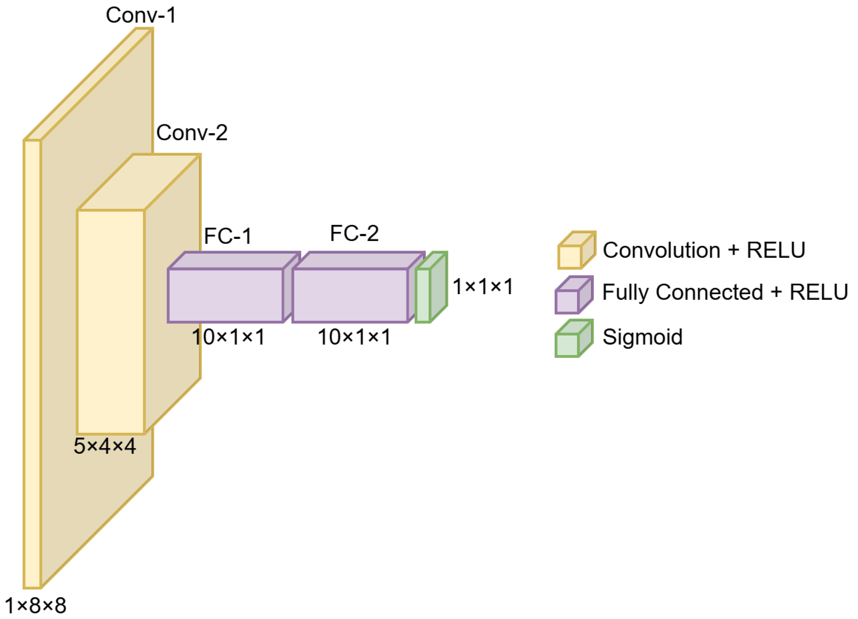
Training and Validation. With the comparative imagery as input data, we utilized convolutional neural networks (CNNs) [19] as the technical method for training music similarity detection models. The overall model structure is an ensemble of K CNN sub-models, each of which was trained to specialize on one of the K selected features. These CNN sub-models shared the same structure as illustrated in Figure 3. All layers including the fully connected layers were implemented as convolutional layers. For every layer, the ReLU activation [20] function was utilized. After using the CNN, the output was passed through a sigmoid function to convert the result into a probability of similarity. Although the network was trained with heatmaps of size $8\times 8$, it can be used to process heatmaps of size greater than $8\times 8$ by acting as a sliding window over a larger heatmap.

Each CNN sub-model was trained independently in order to achieve the best performance for each feature. The hyperparameters considered in the training and validation were learning rate (LR), epochs, and distance metric. To find the optimal values for these parameters and to choose the appropriate distance metric among the ones given in

Table 6. Common distance metrics used in the literature and their definitions [21].

Metric	Definition	Formula
Cosine Similarity	The cosine of the angle between two feature vectors $A=\{a_1,\dots ,a_n\}$ and $B=\{b_1,\dots ,b_n\}$.	$cos\left(\theta \right)={\displaystyle \frac{A·B}{\parallel A\parallel ·\parallel B\parallel }}$
Euclidean Distance	The distance between two feature vectors measured along a straight line.	$d_{L2}(A,B)=\sqrt{{\sum }_{i=1}^n{(a_i-b_i)}^2}$
Manhattan Distance	The distance between two feature vectors measured along orthogonal axes.	$d_{L1}(A,B)={\sum }_{i=1}^n|a_i-b_i|$
Earth Mover’s Distance	A measure of the minimum amount of work required to change one distribution into the other with respect to a feature vector distance metric d.	$d_{EM}(P,Q)={inf}_{\gamma \in \Pi (P,Q)}{\mathbb{E}}_{(x,y)\sim \gamma }\left[d(x,y)\right]$

, we conducted experiments, where each distance metric was tested with a range of suitable values for different parameters. For the training, BCE (binary cross entropy) loss was used with a momentum of 0.9 and a learning rate scheduler with an exponential decay of 0.9 per each epoch. In Section 4, we report our experimental results in relation to hyperparameters and distance metrics.

2.5. Method 4: Ensemble Decision Process

Our early experimentation of the $K=4$ sub-models indicated that they have different strengths and weaknesses. This naturally led to the ensemble approach to enable these sub-models to make similarity decisions collectively. Instead of simple voting or averaging, a Bayesian interpretation was adopted by viewing ensembling as marginalization over sub-models, giving the ensemble prediction

$$p\left(c\right|d)=\sum _{f=1}^{K}p\left(c|M_f\left(d\right)\right)\pi \left(M_f\right),d\in D$$

where c is a prediction (i.e., one of the two class labels “similar” and “dissimilar”), d is a data object in a dataset D, $p\left(c\right|d)$ is the probability for a data object d to result in a prediction c, $M_f$ is a sub-model for feature f, and $p\left(c|M_f\left(d\right)\right)$ is the probability for a sub-model $M_f$ to make a prediction c based on input data object d. The probability $p\left(c|M_f\left(d\right)\right)$ is moderated by $\pi \left(f\right)$, that is, a prior distribution over all feature-based sub-models. Arguably, the most appropriate distribution over models is the posterior with respect to the training data [22]. We can thus obtain $\pi \left(f\right)$ as ensemble weights inductively through the training process:

$$w_{M_f}=\pi \left(M_f\right)=P\left(M_f\right|D)={\displaystyle \frac{P\left(D\right|M_f)P\left(M_f\right)}{P\left(D\right)}}={\displaystyle \frac{exp[-\tau ·LL\left(M_f\right)]}{{\sum }_{j=1}^{K}exp[-\tau ·LL\left(M_j\right)]}}$$

where each sub-model $M_f$ is assigned a weight according to its likelihood to make a correct prediction in relation to the other sub-models. The weight $w_{M_f}=\pi \left(M_f\right)$ can be derived from the training loss. The fraction on the right expresses the relation between a sub-model $M_f$ and other sub-models. The log-likelihood function, $LL\left(M_f\right)$ is typically moderated by a factor $\tau$. We applied a heuristic (strongly related to shrinkage) to encourage shrinkage towards uniform weights to maximize the ensemble benefit and prevent a single model from dominating the resulting heatmap. Through our experimentation, we determined $\tau =0.2$ empirically. We will report the training results about the weights further in Section 4.

2.6. System Architecture

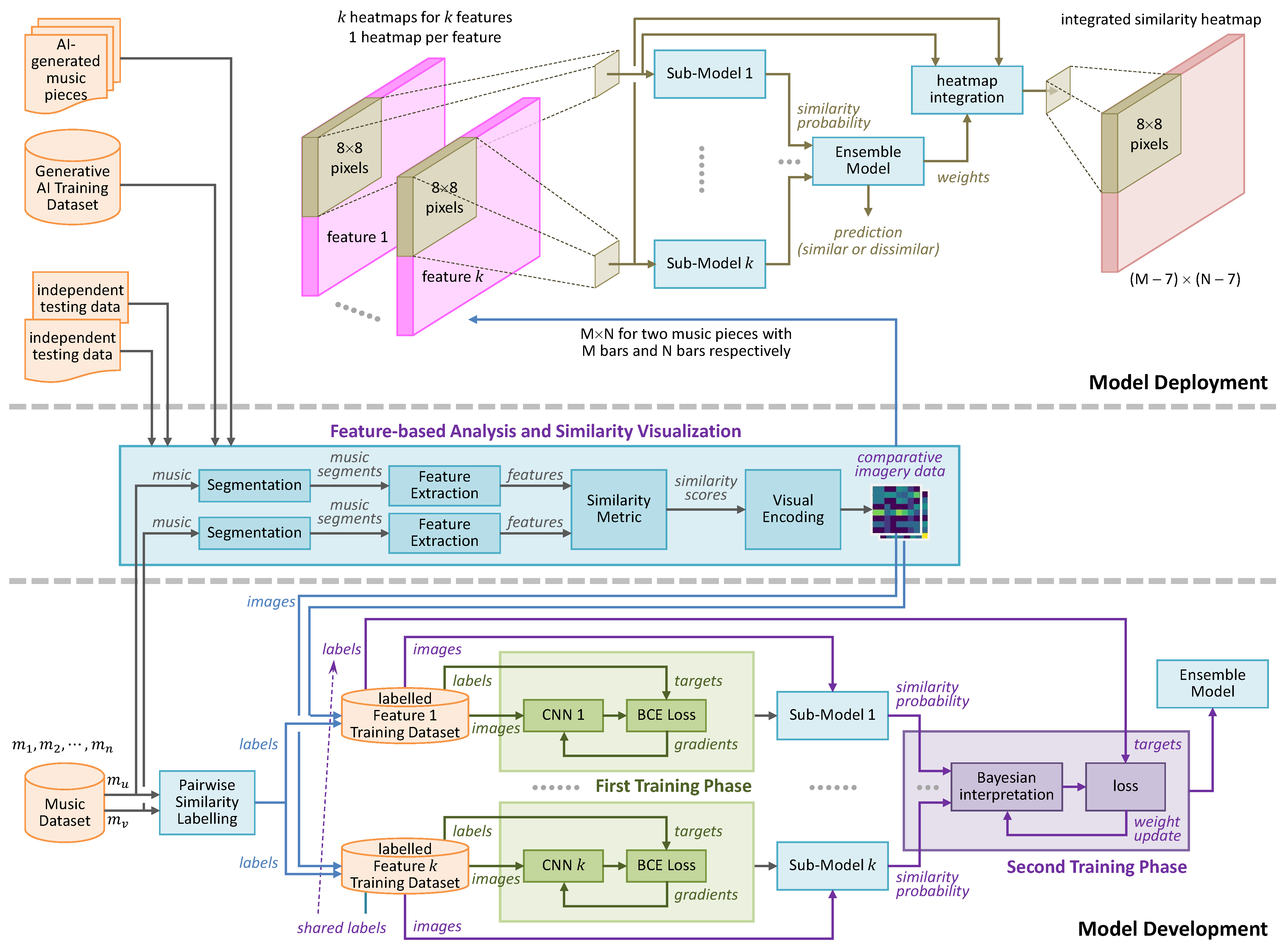
Figure 4 outlines the overall architecture of the technical environment that was used to conduct this research. In particular, the lower part of the figure shows the part of the environment for the training and validation of feature-based sub-models and the ensemble model. The upper part of the figure shows the part of the environment designed for deploying the trained model to test AI-generated music pieces, which were not used in the development phase. In Section 4, we report the results of testing these AI-generated music pieces, confirming that the ensemble model trained in the development phase can positively detect similarity in AI music pieces.

The middle part of the figure shows the technical components for feature-based analysis and heatmap generation, which support both the model development and deployment phases while allowing humans to visualize intermediate results.

3. Experimental Results: Validating the Framework

In this section, we report the results obtained from applying feature-based analysis and visualization methods to a number of songs in order to gain an understanding as to the relationship between music feature similarity and music similarity in the context of copyright infringement and plagiarism. It is not difficult to postulate that some features are more indicative than others. However, to the best of our knowledge, there a systematic experiment has yet to be reported in the literature. We thereby designed and conducted a systematic experiment on the 33 features in Table 1, Table 2, Table 3, Table 4 and Table 5 in conjunction with several songs.

Given a particular piece of music, one can apply some changes to the music to generate its variations. For example, consider the traditional song “Happy Birthday” ⯈ (https://github.com/asaner7/imagery-music-similarity/blob/main/songs-in-paper/HappyBirthday_mp3.mp3, accessed on 30 May 2025). We created its variations on MuseScore 4.2.1 [23], characteristically representing different forms of modification. Nevertheless, the modification was not sufficient enough to make any of these variations to be considered to be a different song. The variations created for “Happy Birthday” include the following: transpose ⯈ (https://github.com/asaner7/imagery-music-similarity/blob/main/songs-in-paper/HappyBirthday_Transpose.mp3, accessed on 30 May 2025), chord-change ⯈ (https://github.com/asaner7/imagery-music-similarity/blob/main/songs-in-paper/HappyBirthday_Chord.mp3, accessed on 30 May 2025), genre change (specifically swing in this case) ⯈ (https://github.com/asaner7/imagery-music-similarity/blob/main/songs-in-paper/HappyBirthday_Swing.mp3, accessed on 30 May 2025), grace notes and other embellishments ⯈ (https://github.com/asaner7/imagery-music-similarity/blob/main/songs-in-paper/HappyBirthday_Ornamental.mp3, accessed on 30 May 2025), and a combination ⯈ of several of these changes (https://github.com/asaner7/imagery-music-similarity/blob/main/songs-in-paper/HappyBirthday_Combo.mp3, accessed on 30 May 2025).

We intentionally avoided any preconception or biases by treating all 33 features consistently in our feature-based analysis and visualization. Each feature is defined upon a segment of 1 bar long. The MIDI file of each variation is limited to 8 bars, resulting in 8 feature values for 8 segments. The heatmaps for comparing any two songs or variations are all of $8\times 8$ resolution. Different distance metrics were experimented (Table 6). The figures in this section show only the results of the negative L1 norm (Manhattan distance). The pixels were all color-coded using the same color-coding scheme, with bright yellow for higher similarity and dark blue for higher dissimilarity. All of the heatmaps associated with the same feature have the same color-mapping function. All seven histogram-based features in Table 1, Table 2, Table 3, Table 4 and Table 5 were scaled between [−2,0] where all other features were scaled between [−3,0] to ensure maximum contrast for visual inspection. As mentioned in Section 2.4, the color-coding does not affect the machine learning processes as only the original numerical matrices (before visualization) were used in training, validation, and testing.

3.1. Melodic Features

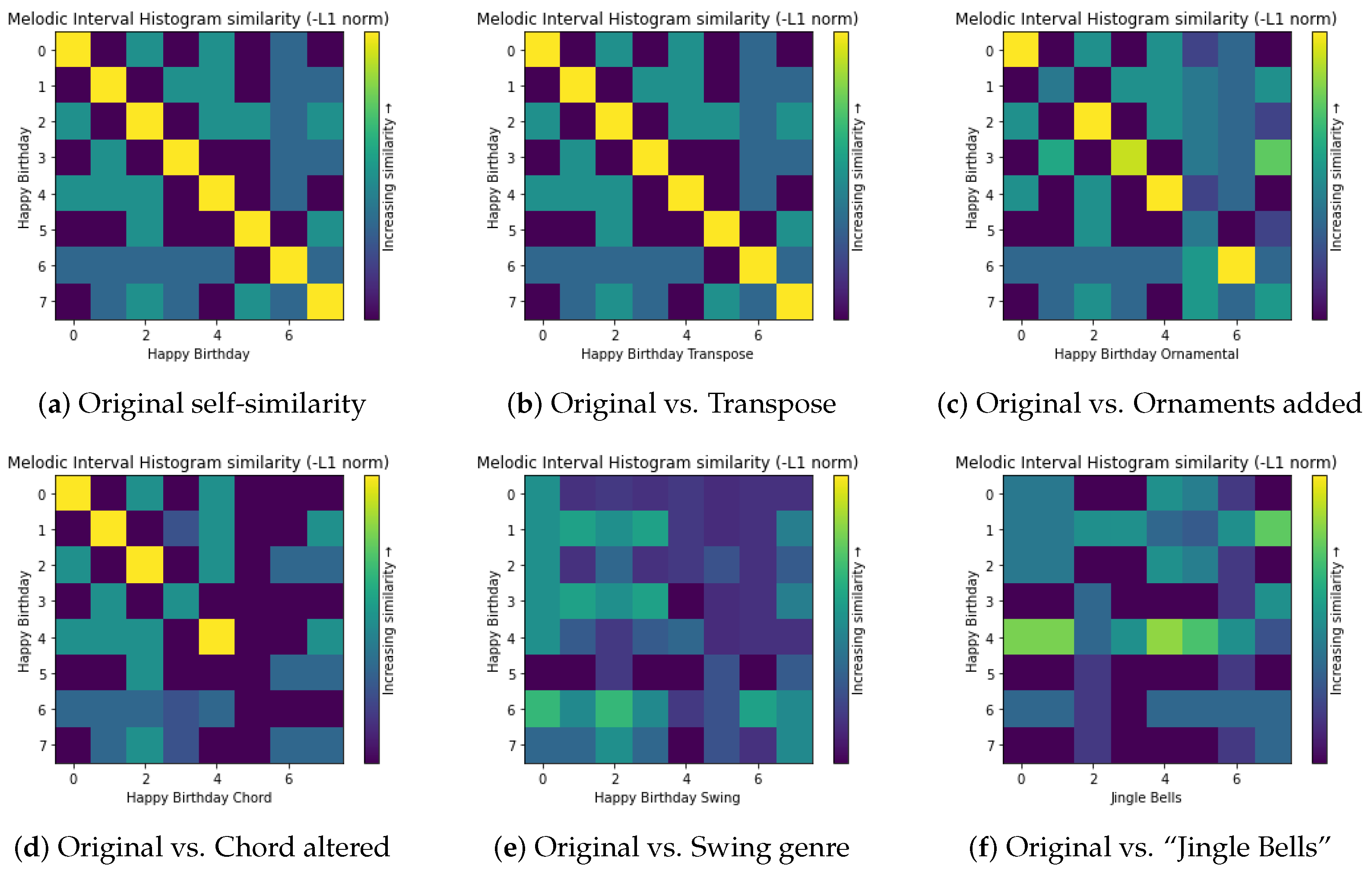
In the literature, melodic features have been used to detect similarity. Our experiments confirmed, largely, the usefulness of the melodic feature. Figure 5 shows six heatmaps illustrating the use of the melodic interval histogram to compare “Happy Birthday” with itself (a), four variations (b, c, d, e), and “Jingle Bells” ⯈ (https://github.com/asaner7/imagery-music-similarity/blob/main/songs-in-paper/JingleBells.mp3, accessed on 30 May 2025) (f). There were also comparisons with other types of variations and many other songs, and these six heatmaps are examples demonstrating the indicative power of the melodic feature.

As shown in Figure 5a, a self-similarity heatmap of this feature usually has a diagonal line of bright pixels, which serves as a baseline reference for observing dissimilar patterns in other heatmaps. The transpose manipulation maintains such a pattern as shown in Figure 5b; hence, this type of variation will be considered as similar to the feature of the melodic interval histogram.

From Figure 5c, we can see that the addition of ornaments to each bar of the song did not change the heatmap drastically, and substantial similarity is still obvious. In Figure 5d, it is clear that the addition of chords to each bar affected the heatmap more in comparison with Figure 5c; the overall melodic similarity has still been captured, but the changes in the bars at the end were not detected, which suggests some weakness of the feature.

Figure 5e indicates a major weakness of the feature of the melodic interval histogram in detecting genre changes, as there are no bright patterns at all. This suggests that genre changes might fool an ML model that relies too heavily on this feature. However, this observation may be biased by visual inspection. An ML model can still potentially learn to recognize other subtle patterns. Nevertheless, the risk should not be dismissed.

In Figure 5f, we can observe some bright pixels, suggesting melodic similarity in the bars concerned. These bright patterns appear in different regions of the heatmap and do not form a diagonal line or a block of pixels. This suggests that the similarity is either in an isolated location (e.g., location [$x=7,y=1$]) or related to a single bar (e.g., [y = 4]).

The other melodic features in Table 1 did not result in heatmaps as effective as the melodic interval histogram. The resultant heatmaps were either completely bright or there was almost no difference between similar cases (i.e., variations of “Happy Birthday” ) and dissimilar cases (i.e., “Jingle Bells” and some other songs). We therefore prioritize the melodic interval histogram for our data collection and ML development effort.

3.2. Pitch Statistics Features

Among the eight features in Table 2, only the folded fifths pitch class histogram showed some promising results. This feature is expected to be a complementary feature in the similarity detection model, since having similar pitch properties between two music pieces is not compelling enough to claim plagiarism. However, it is possible that alongside the melodic interval histogram, it may provide more evidence for an alleged plagiarism. 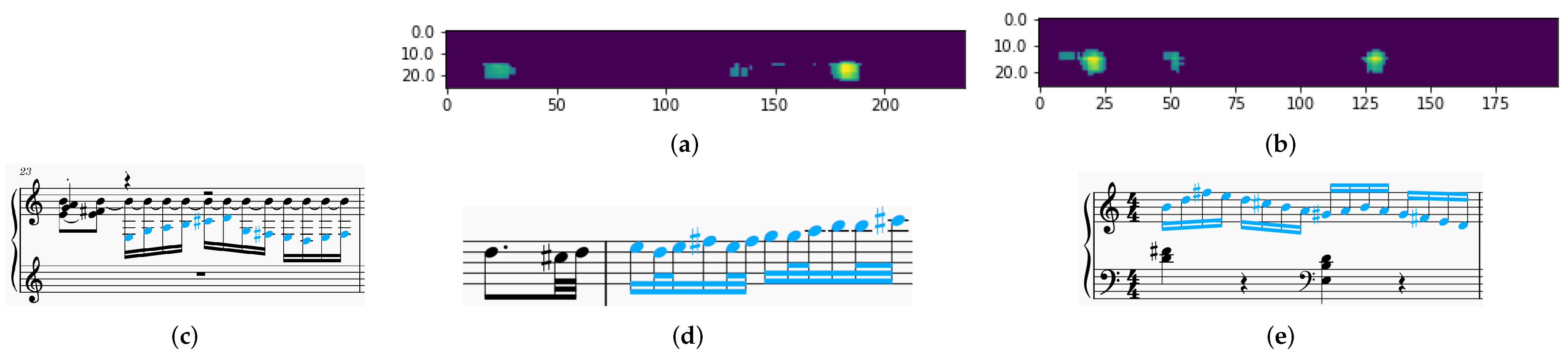Figure 6 shows the performance of this feature on the swing version of “Happy Birthday”, where the visual patterns depicted are more interesting than Figure 5e. This suggests that the feature of folded fifths pitch class histogram may potentially aid in the detection of similarity for this challenging type of variation.

3.3. Chords and Vertical Interval Features

Harmony may potentially be a useful aspect of music in similarity detection. Our experiments provided strong evidence in supporting this hypothesis. In particular, the features wrapped vertical interval histogram and distance between two most common vertical intervals performed well. Particularly, the distance between two most common vertical intervals performed well with the swing variation. The harmony, similar to pitch statistics, can provide supplementary evidence for similarity detection. Figure 7 shows some of the results obtained with the feature of distance between two most common vertical intervals. We can easily observe that Figure 7e shows a very strong indication of similarity.

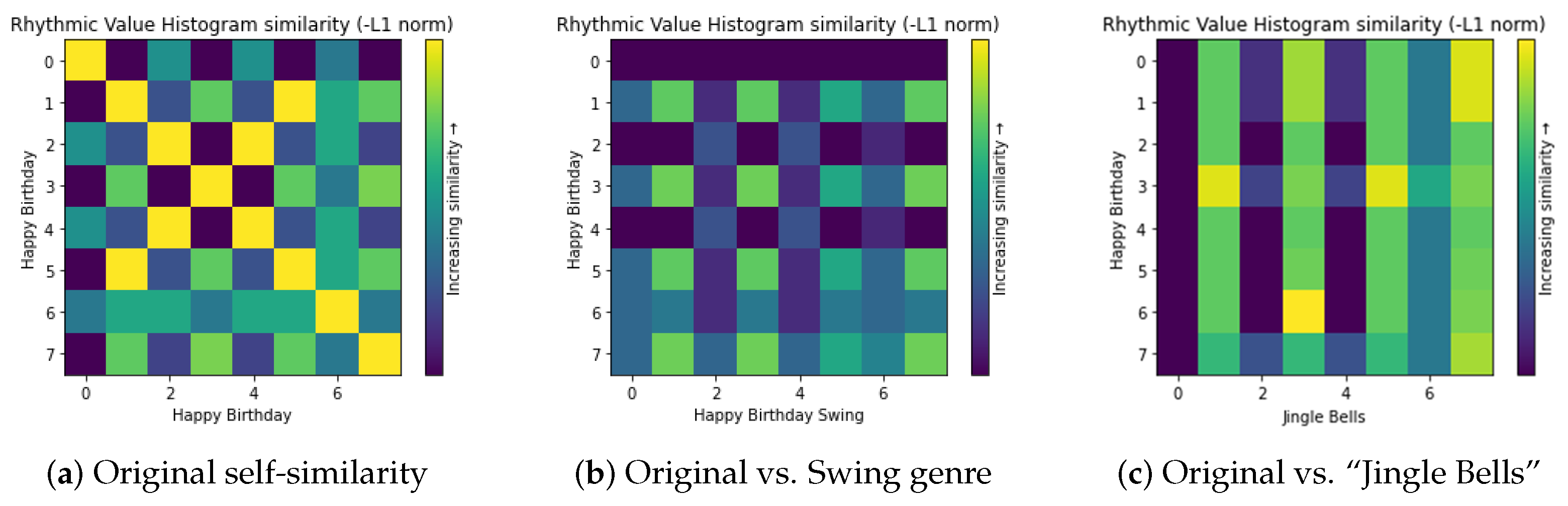
3.4. Rhythm and Beat Features

Through experimentation, we found that the seven rhythm and beat features in Table 4 did not adequately support similarity detection. This is understandable, since two different songs could potentially have the same rhythm, which would not be considered as plagiarism. There could also be cases where a variation of a song could have a different rhythm while still being the same song, e.g., the swing variation of “Happy Birthday”. As an example, Figure 8 shows three comparative heatmaps, indicating that the feature of rhythmic value histogram cannot distinguish between (b) being similar and (c) being dissimilar. Therefore, we did not prioritize any feature in Table 4 for data collection and model development in this work.

3.5. Texture Features

Our experiments showed that the four texture features in Table 5 were not indicative in similarity detection. It is understandable as the motion of voices present in a music piece is not a characteristic that is normally used to distinguish similar pieces from dissimilar ones. For example, Figure 9 shows three heatmaps with most pixels in bright yellow and some in bright green regardless of the songs being compared. Therefore, we did not prioritize any feature in Table 5 for data collection and model development in this work.

3.6. Findings from the Experimental Results

In addition to “Happy Birthday” and “Jingle Bells”, we also experimented with other songs. The overall experimental results of the feature-based analysis and visualization have shed light on which features may have strong association with similarity detection in the context of copyright infringement and plagiarism. Among the thirty-three features studied, most do not have such strong association, e.g., the seven rhythm and beat features in Table 4 and four texture features in Table 5. For these two groups of features, the findings are consistent with the general understanding as to what may contribute to the judgment of music plagiarism.

We have identified four features that have stronger indicative power than others. They are (i) melodic interval histogram, (ii) folded fifths pitch class histogram, (iii) wrapped vertical interval histogram, and (iv) distance between two most common vertical intervals. These features are all transpose-invariant and can detect similarity to an adequate extent where different chords and embellishments are added to create variations of a music piece. Moreover, when a combination of these alterations were applied to the original version of a music piece, the performance of these features did not deteriorate.

The type of swing-genre variations has been found to be a challenge for identifying similarity visually. Nevertheless, this provided us with stronger motivation to train ML models and to investigate whether the patterns resulting from such variations could indeed be detected by ML models even though they are not too obvious to the human eye. These experiments also inspired us to use comparative imagery as input data to train ML models for similarity detection. Since humans cannot visually assess thousands of heatmaps in order to compare one piece of music with many songs in a data repository, a good-quality ML model would be significantly more cost-effective. Meanwhile, as the judgment of plagiarism is a highly sensitive matter, it is necessary for humans to be able to scrutinize and interpret the judgment of any ML model for similarity detection. Hence, being able to visualize the feature-based comparative imagery allows explainable AI to support such scrutiny and interpretation.

4. Experimental Results: Model Training, Validation, and Testing

The datasets used in the experiments reported in Section 4.1, Section 4.2, and Section 4.4 are available on GitHub (https://github.com/asaner7/imagery-music-similarity, accessed on 30 May 2025).

4.1. Machine Learning Experiments

Like many ML workflows, we conducted numerous experiments to optimize various hyperparameters. For the four sub-models corresponding to the four features identified (Section 3),

Table 7. Summary of model performance with respect to different combinations of the specified hyperparameters using validation metrics. The abbreviations of the feature names are MI (melodic interval), FFPC (folded fifths pitch class), WVI (vertical interval), and DBTMCVI (distance between two most common vertical intervals).

Feature	Metric	Loss	F1 Score	Accuracy	AUC	LR	Epochs
MI Histogram	Earth Mover’s Distance	0.08	0.90	0.97	0.99	0.005	300
FFPC Histogram	Earth Mover’s Distance	0.10	0.94	0.98	0.99	0.005	100
WVI Histogram	Earth Mover’s Distance	0.08	0.99	1.00	1.00	0.01	100
DBTMCVI Heatmap	L1 Norm	0.12	0.94	0.98	0.99	0.01	200

shows the best combination obtained for training each of the four sub-models.

The results of the experiments showed that Earth mover’s distance calculated with respect to the L1 norm performed the best with the three histogram features, and L1 norm worked the best for the feature of distance between the two most common vertical intervals. Moreover, since the distance between the two most common vertical intervals is a scalar feature, Earth mover’s distance is not meaningfully applicable and was not considered as an option for this feature.

The individual validation performance of each feature-based sub-model is also summarized in Table 7, along with chosen training hyperparameters. Figure 10 shows that all models clearly train properly and converge to optimal parameters within the number of epochs allocated to training in each case. Overfitting is also demonstrably avoided, which is expected due to the use of an L2 regularizer and dropout.

Lastly, the confusion matrix of each CNN is given in Figure 11, where the accuracy measures of the four sub-models in the validation stage are displayed. Each sub-model can separate between classes almost perfectly, which can be inferred from the area under the receiver operator characteristic curve (AUC). All features have an almost perfect AUC score and a negligible classification error. However, this almost perfect performance does not mean that (i) all four sub-models are in agreement for every pixel location in a set of feature-based input heatmaps, and (ii) their performance in independent testing is not assured since the sub-models are not trained with any legally verified data.

The performance of the ensemble model on the same validation set used in validation-testing the individual sub-models is better than the individual performance of each sub-model in terms of all validation metrics as shown in

Table 8. Summary of model ensemble performance on the same validation set used in the training of the individual models. Feature names are abbreviated.

Results: Ensemble Model
Loss	0.06
F1 Score	1.00
Accuracy	1.00
AUC	1.00
Feature Weights:
MI Histogram	0.39
FFPC Histogram	0.20
WVI Histogram	0.33
DBTMCVI	0.08

. The confusion matrix in in Figure 12 also shows that the ensemble model has achieved a faultless classification of the heatmaps in the validation set. Therefore, enabling different feature-specific sub-models to make collective decisions is clearly beneficial to similarity detection.

4.2. Testing with Independent Data

In order to test the ensemble model and its sub-models, we selected two pieces of music that differ significantly from the training data. One is a Chinese folk song called “Mo Li Hua” (Jasmine Flower), which dates back to the 18th century. The song has multiple verses, each with the same basic melodic and rhythmic structure. Its melody is gentle, graceful, and lyrical. The other is a Turkish march called “Izmir Marsi” (Izmir March), dating back to the period of the Turkish War of Independence (1919–-1923). It is a fast paced, bold, and highly energetic song. The march has a main melody and accompanying counter melodies, and these are repeated throughout the song.

For each of the two pieces of music, we selected eight bars as the original version and created five variants, namely (a) transpose, (b) chord altered, (c) swing genre, (d) ornaments added, and (e) combination of several of these changes. Let us denote the original “Mo Li Hua” and its five variants as $C_o,C_a,C_b,C_c,C_d,C_e$, and those of “Izmir Marsi” as $T_o,T_a,T_b,T_c,T_d,T_e$. With the 12 music pieces, there are 66 pairwise comparisons, among which 30 are similar (positive) and 36 are dissimilar (negative).

Table 9. The results of testing the four sub-models and the ensemble model with independent testing data that differ from the training data significantly. The percentage values are normalized based on the class size, i.e., TP/(TP + FN), FP/(TN + FP), TN/(TN + FP), or FN/(TP + FN). The abbreviations of feature names are MI (melodic interval), FFPC (folded fifths pitch class), WVI (vertical interval), and DBTMCVI (distance between two most common vertical intervals).

Model	TP	FP	TN	FN	Precision	Recall	Accuracy	F1 Score
MI Histogram	25 (83.3%)	4 (11.1%)	32 (88.9%)	5 (16.7%)	0.862	0.833	0.864	0.847
FFPC Histogram	21 (70.0%)	10 (27.8%)	26 (72.2%)	9 (30.0%)	0.677	0.700	0.712	0.689
WVI Histogram	27 (90.0%)	2 (5.6%)	34 (94.4%)	3 (10.0%)	0.931	0.900	0.924	0.915
DBTMCVI	19 (63.3%)	13 (36.1%)	23 (63.9%)	11 (36.7%)	0.594	0.633	0.636	0.613
Ensemble	28 (93.3%)	3 (8.3%)	33 (91.7%)	2 (6.2%)	0.903	0.933	0.924	0.918

shows the results of applying the four sub-models and the ensemble model to heatmaps depicting these 66 pairwise comparisons.

From Table 9, we can observe that the ensemble model has performed the best in dealing with music data that differ significantly from the training data. It is closely followed by the WVI (vertical interval) sub-model, then MI (melodic interval), FFPC (folded fifths pitch class), and DBTMCVI (distance between two most common vertical intervals). Among the 66 pairwise comparisons, there are ten cases where MI and WVI sub-models disagree with each other. In eight (out of ten) cases, the FFPC sub-model helps the ensemble model to make correct decisions. The testing provided concrete validation evidence, confirming that training ML models with comparative imagery data can produce effective models for determining music similarity.

4.3. Testing with Known Plagiarism Data

The model can now be tested with known plagiarism data. In Section 2.3, we discussed one such case, “Under Pressure” vs. “Ice Ice Baby”. Figure 13a shows the similarity patterns detected by our ensemble model, which compared two songs using a 2D sliding window of $8\times 8$ bars and created an output heatmap. In other words, each pixel in this heatmap corresponds to an 8 × 8 pixel block in the original feature-based heatmap at the resolution of one bar per pixel. For human visualization, this model output is then dilated to recover the locations of the regions of similarity in the songs as shown in Figure 13b, where the similarity mask is thresholded to reduce the visibility of pixels with low similarity values. We can compare this with the original weighted-sum heatmap shown in Figure 2b; Figure 13b, which is referred to as an ensemble similarity mask, identifies all the critical regions shown in Figure 2b while allowing humans to focus on these regions more quickly and easily.

One important benefit of using comparative imagery as the input and output of a model for music similarity detection is that humans can review the input and output more intuitively. Figure 13c–f show four individual feature-based comparative heatmaps that are inputs to the four feature-based sub-models, respectively. We can observe that the ensemble output in Figure 13a does not solely depend on one feature. From the top to bottom of the image, the following can be observed:

• The first long line of bright dots ($y\approx 0$) is related to the corresponding bright patterns in (c, d).
• The second long line of bright dots ($y\approx 35$) corresponds to the bright patterns in (c, d, e).
• The short line of dots on the center–left ($y\approx 60$) corresponds to the bright patterns in (c), where the bright patterns span across the entire heatmap horizontally. It is interesting that the ensemble model considered only the small part on the left.
• The third long line of bright dots ($y\approx 70$) corresponds to (d).
• The fourth long line of bright dots ($y\approx 120$) corresponds to (c, d, e).
• The input heatmap in (f) does not contribute to the horizontal-line pattens shown in (a).
• Input heatmaps (c, d) show four vertical strips, while input heatmaps (e, f) show three vertical strips. For the left part of heatmaps ($x<20$), the ensemble model was more influenced by (c, d).
• The bright spot on the bottom-left of (c) did not trigger a positive reaction in (a), suggesting that the ensemble model does not completely rely on the melodic feature.

These observations demonstrate that our approach can provide a means to improve the explainability of AI.

4.4. Testing with AI-Generated Music

The increasing prevalence of generative AI models has raised concerns over copyright infringement. In this work, we used Google Magenta 2.1.2 [24] to create a music dataset for testing our trained models, and in particular, the ensemble model. Google Magenta has two generative AI models, MusicVAE and Music Transformer. At the moment, it is the only generative music tool whose source code, specifically the Transformer model, is available in the public domain.

Both models were trained using a classical music dataset called Maestro, which contains virtuosic piano performances of piano pieces by famous composers throughout history. This dataset was created by Hawthorne et al. [25]. Yin et al. [26,27,28] discussed the originality of the music generated by their model trained using the source code of Google Magenta and the Maestro dataset (1275 music pieces, around 200 h) [25]. They found some cases of chunks of music being copied from the training data in the generated music. The dataset by Hawthorne et al. is referred to as the CPI dataset and can be found at their website [29].

We trained two generative AI models, VAE and Transformer, using the source code of Google Magenta, the CPI dataset by Hawthorne et al. [25], and the same hyperparameters used by Yin et al. [26,27,28] in training their model. We applied our similarity detection model to a number of excerpts generated by the VAE and Transformer models. These excerpts are labeled as V-CPI-# or T-CPI-#, indicating the generative AI model (V for VAE or T for Transformer) trained by us and the training dataset CPI by Yin et al. [26,27,28] Figure 14 shows eight examples of music pieces generated using the Transformer and VAE with four examples from each, which were tested against all 1275 music pieces in the CPI dataset. We can observe bright patterns in these heatmaps, indicating the possible similarity regions. The heatmaps enable humans to focus on these regions without much effort, demonstrating the informativeness and the effectiveness of data visualization in aiding humans in their processes of evaluating, scrutinizing, and interpreting model outputs.

Let us examine one particular case closely. Figure 15 shows two testing results after comparing an AI-generated music piece using the Transformer model. Our similarity detection model found a few pieces in the training data, i.e., the CPI dataset. Two of these pieces, both by Beethoven, were examined closely. When comparing with T-CPI-1 with the 1275 pieces in the CPI dataset, the ensemble model scored both pieces with the highest similarity score of 0.92, which correspond to the brightest regions in the heatmaps as shown in Figure 15a,b. The repeating bright regions have almost identical musical properties and are repeated in Beethoven’s pieces. An interesting finding is that the highlighted regions correspond to approximately the same part of the AI-generated piece. This may be partly because T-CPI-1 is a relatively short piece and does not contain many repeated musical properties. The piece for the most part has many convoluted bars and unrealistic chord progressions which makes it distinctly different from the training data, and possibly only the highlighted region in the piece diverts from this behavior.

Upon listening to the three excerpts mentioned above, they in fact have a similar feel, which stems from the common melodic progressions between the pairs concerned as well as across all three. There are fairly distinguishable runs in all three excerpts, which can be heard easily by the human ear. In music, a run indicates a note progression consisting of adjacent notes played in a successive manner with usually one or two semitones between each note. Some examples of such runs present in the excerpts are given in Figure 15c–e. Normally, such similarity in music is not considered as copying. While the model has rightly identified such similarity patterns, it requires humans to interpret the patterns using their knowledge that is currently not present in the training data.

The melodic interval histogram for these bars would look reasonably similar since the melodic structure is almost the same even if the notes are different. This is because the intervals between the notes do not change across the melodic progression of the run, which allows the model to detect the similar nature of these features in the pieces. This is an indication that the model can detect not only exact replicas of melodic structures in musical pieces, but it can also detect even more generalized cases of similarities in the compared pieces. One implication of this model behavior is that it can serve as a warning mechanism for similarity patterns that could potentially infringe copyright, while leaving the final interpretation to human experts.

5. Conclusions

In music, plagiarism has been an important but troubled issue, which becomes even more critical with the widespread usage of generative AI tools. Meanwhile, the development of techniques for music similarity detection has been hampered by many challenges, including the three challenges discussed in Section 1. In this paper, we addressed these three challenges by bringing feature-based analysis and visualization into the ML workflow to develop models for music similarity detection, i.e., addressing C1 by gaining better understanding of the relationship between music feature similarity and music similarity in the context of copyright infringement and plagiarism; addressing C2 by providing the ML workflow with comparative imagery as a new form of data in training and testing; and addressing C3 by allowing humans to scrutinize and interpret model predictions through intermediate visualization data. In addition, we substantiated our approach using information-theoretical reasoning, created a dataset for training and validation while keeping legally validated data for testing, utilized CNNs and Bayesian interpretation for developing ML models, and applied our trained model to AI-generated music as well as legally validated data.

Although we have found several methods to address the three challenges, it does not in any way mean that these problems have been solved. More research and development will be necessary to address these and other challenges in music similarity detection. In particular, there is a general need to develop deeper theoretical understanding and practical methods for developing ML models with sparse data. Our experiments focused on certain song-type genres, and there are many different music genres to be studied, possibly using our approach or other approaches. In future work, we will expand our training and validation dataset as well as the collection of AI-generated music for testing. We also plan to apply a recent solution for dealing with data scarcity in image similarity analysis [30] to music similarity analysis by exploring ensemble models built from genre-specific sub-models.

References and Notes

1. Wilde, O. Imitation Is the Sincerest Form of Flattery That Mediocrity Can Pay to Greatness, circa 1890. Widely attributed to Oscar Wilde, though no definitive source confirms it in his published works.
2. UK Government. Copyright and Artificial Intelligence. 2024. Available online: https://www.gov.uk/government/consultations/copyright-and-artificial-intelligence/copyright-and-artificial-intelligence (accessed on 18 April 2024).
3. Knees, P.; Schedl, M. A survey on music similarity and recommendation from music context data. ACM Trans. Multimed. Comput. Commun. Appl. 2013, 10, 1–21. [Google Scholar] [CrossRef]
4. Schedl, M.; Pohle, T.; Knees, P.; Widmer, G. Exploring the music similarity space on the web. ACM Trans. Inf. Syst. 2011, 29, 1–24. [Google Scholar] [CrossRef]
5. Karydis, I.; Lida Kermanidis, K.; Sioutas, S.; Iliadis, L. Comparing content and context based similarity for musical data. Neurocomputing 2013, 107, 69–76. [Google Scholar] [CrossRef]
6. Spärck Jones, K. A Statistical Interpretation of Term Specificity and Its Application in Retrieval. J. Doc. 1972, 28, 11–21. [Google Scholar] [CrossRef]
7. Beel, J.; Gipp, B.; Langer, S.; Breitinger, C. Research-paper recommender systems: A literature survey. Int. J. Digit. Libr. 2015, 17, 305–338. [Google Scholar] [CrossRef]
8. Malandrino, D.; De Prisco, R.; Ianulardo, M.; Zaccagnino, R. An adaptive meta-heuristic for music plagiarism detection based on text similarity and clustering. Data Min. Knowl. Discov. 2022, 36, 1301–1334. [Google Scholar] [CrossRef]
9. De Prisco, R.; Malandrino, D.; Zaccagnino, G.; Zaccagnino, R. A computational intelligence text-based detection system of music plagiarism. In Proceedings of the 2017 4th International Conference on Systems and Informatics (ICSAI), Hangzhou, China, 11–13 November 2017; pp. 519–524. [Google Scholar] [CrossRef]
10. Li, T.; Ogihara, M. Content-based music similarity search and emotion detection. In Proceedings of the 2004 IEEE International Conference on Acoustics, Speech, and Signal Processing, Montreal, QC, Canada, 17–21 May 2004; Volume 5, pp. V-705–V-708. [Google Scholar] [CrossRef]
11. Nguyen, P.; Le, H.; Bui, V.; Chau, T.; Tran, V.; Bui, T. Detecting Music Plagiarism Based on Melodic Analysis. J. Inf. Hiding Multimed. Signal Process. 2023, 14, 75–86. [Google Scholar]
12. Nair, R.R. Identification and Detection of Plagiarism in Music using Machine Learning Algorithms. Master’s Thesis, National College of Ireland, Dublin, Ireland, 2021. [Google Scholar]
13. Chen, M.; Golan, A. What may visualization processes optimize? IEEE Trans. Vis. Comput. Graph. 2016, 22, 2619–2632. [Google Scholar] [PubMed]
14. Chen, M. Cost-Benefit Analysis of Data Intelligence–Its Broader Interpretations. In Advances in Info-Metrics: Information and Information Processing across Disciplines; Oxford University Press: Oxford, UK, 2020; pp. 433–463. [Google Scholar]
15. Tam, G.K.L.; Kothari, V.; Chen, M. An analysis of machine- and human-analytics in classification. IEEE Trans. Vis. Comput. Graph. 2017, 23, 71–80. [Google Scholar] [PubMed]
16. McKay, C. jSymbolic Manual. 2018. Available online: https://jmir.sourceforge.net/manuals/jSymbolic_manual/home.html (accessed on 17 January 2024).
17. Abdul-Rahman, A.; Roe, G.; Olsen, M.; Gladstone, C.; Whaling, R.; Cronk, N.; Morrissey, R.; Chen, M. Constructive visual analytics for text similarity detection. Comput. Graph. Forum 2017, 36, 237–248. [Google Scholar]
18. Ye, Z.; Chen, M. Visualizing ensemble predictions of music mood. IEEE Trans. Vis. Comput. Graph. 2023, 29, 864–874. [Google Scholar] [PubMed]
19. LeCun, Y.; Boser, B.; Denker, J.; Henderson, D.; Howard, R.; Hubbard, W.; Jackel, L. Handwritten Digit Recognition with a Back-Propagation Network. In Proceedings of the 3rd International Conference on Neural Information Processing Systems, Denver, CO, USA, 27–30 November 1989. [Google Scholar]
20. Fukushima, K. Cognitron: A self-organizing multilayered neural network. Biol. Cybern. 1975, 20, 121–136. [Google Scholar] [CrossRef] [PubMed]
21. Rubner, Y.; Tomasi, C.; Guibas, L.J. The Earth Mover’s Distance as a Metric for Image Retrieval. Int. J. Comput. Vis. 2000, 40, 99–121. [Google Scholar] [CrossRef]
22. Hamid, S.; Wan, X.; Jørgensen, M.; Ru, B.; Osborne, M. Bayesian Quadrature for Neural Ensemble Search. arXiv 2023, arXiv:2303.08874. [Google Scholar]
23. MuseScore Ltd. MuseScore Studio. 2024. Available online: https://musescore.org/en (accessed on 21 February 2024).
24. Google Magenta Team. Magenta: Music and Art Generation with Machine Intelligence. 2022. Available online: https://github.com/magenta/magenta (accessed on 10 November 2023).
25. Hawthorne, C.; Stasyuk, A.; Roberts, A.; Simon, I.; Huang, C.Z.A.; Dieleman, S.; Elsen, E.; Engel, J.; Eck, D. Enabling Factorized Piano Music Modeling and Generation with the MAESTRO Dataset. In Proceedings of the International Conference on Learning Representations, New Orleans, LA, USA, 6–9 May 2019; Available online: https://openreview.net/forum?id=r1lYRjC9F7 (accessed on 10 November 2023).
26. Yin, Z.; Reuben, F.; Stepney, S.; Collins, T. Measuring When a Music Generation Algorithm Copies Too Much: The Originality Report, Cardinality Score, and Symbolic Fingerprinting by Geometric Hashing. SN Comput. Sci. 2022, 3, 340. [Google Scholar] [CrossRef]
27. Yin, Z.; Reuben, F.; Stepney, S.; Collins, T. Deep learning’s shallow gains: A comparative evaluation of algorithms for automatic music generation. Mach. Learn. 2023, 112, 1785–1822. [Google Scholar] [CrossRef]
28. Yin, Z.; Reuben, F.; Stepney, S.; Collins, T. “A Good Algorithm Does Not Steal—It Imitates”: The Originality Report as a Means of Measuring When a Music Generation Algorithm Copies Too Much. In Artificial Intelligence in Music, Sound, Art and Design: 10th International Conference, EvoMUSART 2021, Held as Part of EvoStar 2021, Virtual Event, 7–9 April 2021, Proceedings; Springer: Cham, Switzerland, 2021; pp. 360–375. [Google Scholar] [CrossRef]
29. Google Magenta. MAESTRO Dataset. 2024. Available online: https://magenta.tensorflow.org/datasets/maestro (accessed on 10 November 2024).
30. Liao, Z.; Chen, M. Image similarity using an ensemble of context-sensitive models. In Proceedings of the KDD ’24: Proceedings of the 30th ACM SIGKDD Conference on Knowledge Discovery and Data Mining, Barcelona, Spain, 25–29 August 2024; pp. 1758–1769. [Google Scholar]
Figure 1. From an information-theoretic perspective, decomposing a single complex process in (a) into a series of less complex processes in (b) facilitates gradual entropy reduction. This allows humans to inject more knowledge, which may not be in the data, into the development of each component processes, while enabling humans to visualize and interpret the intermediate data during the deployment. The decomposed workflow in (c) enables gradual entropy reduction in music similarity detection, addressing the challenge of data scarcity as well as facilitating explainable AI. The bottom part of (c) shows that other machine- or human-centric processes, including some future technology, can be integrated through the ensemble decision process.
Applsci 15 07706 g001
Figure 2. Comparing the song “Under Pressure” with (a) itself, (b) “Ice Ice Baby” (similar), and (c) “Bitter Sweet Symphony” (dissimilar). These heatmaps were generated in the ensemble decision process (see Section 2.5), and each is a weighted sum of a set of feature similarity heatmaps with the ensemble weights. The temporal steps along the axes are of 1 bar song segments.
Applsci 15 07706 g002
Figure 3. The CNN structure of the K sub-models, one for each selected feature.
Applsci 15 07706 g003
Figure 4. The overall architecture of the technical environment for this research. The lower part of the figure shows the model development workflow, where k feature-based sub-models and an ensemble model are trained in two separate phases. In this work, we selected four features ( k = 4 ) and developed four sub-models. The upper part of the figure shows the deployment workflow, where we tested the ensemble model and its sub-models with different data that are not used in the development workflow. The middle part of the figure shows the functionality that is shared by both workflows.
Applsci 15 07706 g004
Figure 5. The heatmaps of melodic interval histograms comparing “Happy Birthday” with itself (positive reference), four variations, and “Jingle Bells” (negative reference).
Applsci 15 07706 g005
Figure 6. The heatmaps of folded fifths pitch class histogram for comparing “Happy Birthday” with itself (positive reference), its swing-genre variation, and “Jingle Bells” (negative reference).
Applsci 15 07706 g006
Figure 7. The heatmaps of distance between two most common vertical intervals for comparing “Happy Birthday” with itself (positive reference), four variations, and “Jingle Bells” (negative reference).
Applsci 15 07706 g007
Figure 8. Heatmaps of rhythmic value histogram for comparing “Happy Birthday” with itself (positive reference), its swing-genre variation, and “Jingle Bells” (negative reference). The lack of distinguishing power can be observed.
Applsci 15 07706 g008
Figure 9. Heatmaps of similar motion for comparing “Happy Birthday” with itself (positive reference), its swing-genre variation, and “Jingle Bells” (negative reference). The lack of distinguishing power can be observed.
Applsci 15 07706 g009
Figure 10. Plots of training and validation loss against the number of iterations for all of the features.
Applsci 15 07706 g010
Figure 11. Confusion matrices of the validation set for all of the features with the final trained models: (a) melodic interval histogram; (b) folded fifths pitch class histogram; (c) wrapped vertical interval histogram; (d) distance between two most common vertical intervals.
Applsci 15 07706 g011
Figure 12. The confusion matrix for the validation set for the ensemble model.
Applsci 15 07706 g012
Figure 13. The ensemble output can be validated and explained using the individual feature maps of the songs “Under Pressure” and “Ice Ice Baby”. (a) Unprocessed ensemble output. (b) Ensemble similarity mask. (c) Melodic interval histogram. (d) Folded fifths pitch class histogram. (e) Vertical interval histogram. (f) Distance between two most common vertical intervals heatmap.
Applsci 15 07706 g013
Figure 14. Applying the trained ensemble model (with four sub-models) to compare eight AI-generated music pieces with 1275 pieces of music in the CPI database. For each reference piece (vertical), the heatmap has a top-matched piece (horizontal) in the CPI database. (a) V-CPI-2 vs. Prelude and Nocturne for Left Hand, Op. 9 by Alexander Scriabin. (b) V-CPI-3 vs. Fantasies, Op. 116 No. 7 by Johannes Brahms. (c) V-CPI-9 vs. Scherzo No. 2 in B-flat Major, Op. 31 by Frédéric Chopin. (d) V-CPI-13 vs. Sonetto 123 del Petrarca by Franz Liszt. (e) T-CPI-2 vs. Variations and Fugue in E-flat Major, Op. 35, “Eroica” by Frédéric Chopin. (f) T-CPI-7 vs. Variations Serieuses Op. 54 by Felix Mendelssohn. (g) T-CPI-10 vs. Scherzo No. 2 in B-Flat Minor, Op. 31 by Frédéric Chopin. (h) T-CPI-11 vs. Paraphrase de concert sur Rigoletto, S.434 by Franz Liszt.
Applsci 15 07706 g014
Figure 15. Examples of runs that are present in the similar regions of the excerpts of the three pieces. (a) T-CPI-1 (vertical) vs. a piece by Beethoven (horizontal): Sonata No. 5 in A Major, Op. 18, No.5, Op. 131. (b) T-CPI-1 (vertical) vs. a piece by Beethoven (horizontal): Sonata No. 2 in A Major, Op. 2, No.2: IV. Rondo. (c) An excerpt from T-CPI 1. (d) An excerpt from the Beethoven piece in (a). (e) An excerpt from the Beethoven piece in (b).
Applsci 15 07706 g015