1. Introduction
Modern production facilities can enhance their efficiency through the dynamic development of technology and the widespread availability of computerized control systems [
1,
2,
3,
4]. Current technical capabilities enable the implementation of advanced solutions and facilitate access to infrastructure that allows for the direct acquisition of data from industrial and control-measurement devices. The analysis of such data is a starting point for the better understanding of processes and the more effective use of machines, which in turn enable improvements at all levels of plant management.
1.1. Energy Use in Comminution and Classical Foundations
Comminution (crushing and grinding) is the single most energy-intensive step in the mineral value chain, typically accounting for 30–50% of a concentrator’s total electricity demand [
5]. Classical size-reduction theories—Rittinger (1867), Kick (1885), and most influentially, Bond’s Third Theory of Comminution [
6]—remain the analytical bedrock for estimating specific energy requirements via the Work Index concept. Bond’s methodology, together with population–balance modelling developed by Austin and co-workers [
7], provided the foundation for mill dimensioning, throughput forecasting and early control rules.
Building on these theories, researchers at JKMRC and elsewhere created the first digital simulators of grinding circuits, enabling what Lynch later termed “constrained process optimisation” [
8]. The dynamic simulation work of Herbst and Fuerstenau [
9] and Rajamani & Herbst [
10] introduced multi-loop PI control tuning guidelines that are still embedded in many distributed control systems (DCSs). Model-based predictive control (MPC) subsequently emerged as a powerful alternative, offering the explicit handling of process delays and constraints [
11,
12]. These classical contributions form a well-established benchmark against which any claimed improvement—whether evolutionary algorithms, adaptive neuro-fuzzy inference systems, or deep learning—must be rigorously compared.
1.2. Towards Energy-Efficient Grinding Technologies
Over the last three decades, the industry has adopted novel comminution technologies—high-pressure grinding rolls (HPGRs), stirred media mills, and vertical roller mills—that can achieve 10–40% energy savings relative to traditional ball mills [
13,
14]. Complementary advances in liner design and discrete element method (DEM) simulations have improved charge motion and lifter profiles, further lowering specific energy consumption [
15]. Despite these technological gains, operational energy efficiency is still highly sensitive to ore hardness variability, feed size fluctuations, and sub-optimal control actions [
16]. Consequently, the comminution community continues to view real-time optimisation as a major lever for both cost reduction and greenhouse gas mitigation.
1.3. Evolution of Intelligent Control in Mineral Processing
The first wave of “intelligent” controllers relied on expert-system shells that encoded heuristics from senior metallurgists. With the rise of inexpensive computing power, researchers began training shallow artificial neural networks (ANN) to emulate plant responses. Early studies by Mohanta & Sarangi [
17] and Ghorbani et al. [
18] demonstrated that multilayer perceptrons could predict grind size and flotation recovery with errors lower than linear or polynomial regressions. More recent investigations applied deep LSTM architectures to capture longer-horizon dynamics and incorporate machine-vision signals, achieving superior set-point tracking under variable ore blends [
19]. Nevertheless, these data-driven approaches are often criticised for their “black-box” nature and the difficulty of embedding hard process constraints—issues that hybrid models, evolutionary multi-objective optimisation (EMOO) and physics-informed networks attempt to address. Recent studies have further demonstrated the effectiveness of neural networks in modelling and optimising grinding processes. For instance, ref. [
20] applied a hybrid LSTM–MLP model with NSGA-II to optimise robotic grinding, achieving superior trade-offs between energy use and surface quality. The ANN-based prediction of particle size distribution was shown to be accurate across varying conditions in [
21]. A comprehensive framework for the modelling, control, and optimisation of an industrial grinding circuit using neural networks was introduced in [
22]. These works highlight the adaptability of deep and hybrid architectures to nonlinear, delayed, and multivariable systems.
1.4. Deep-Learning—Driven Optimisation Across Energy-Intensive Industries
Artificial neural network and deep learning (DL) techniques have moved far beyond the proof-of-concept stage and are now embedded in real-time digital twins that supervise entire value chains. A recent case study on a gold-flotation plant showed that an encoder–decoder LSTM surrogate can forecast the concentrate grade 30 min ahead with an
of 0.94, enabling feed-forward set-point adjustments and cutting specific energy by 12% [
23]. Similar multivariate, multistep DL surrogates are being ported to grinding circuits and thickener networks, providing mill-wide optimisation layers that are orders of magnitude faster than first-principle simulators.
A complementary thread focuses on predictive maintenance. In a packaging-plant conveyor, a CNN–BiLSTM digital twin flagged 88% of chain-slack and loop-rupture events at least one shift in advance, allowing maintenance planners to halve unplanned stoppages and save 6% of annual electricity consumption [
24]. The study demonstrates how edge-deployed DL models can operate under strict latency budgets (<10 ms) while streaming thousands of sensor tags over private 5G.
Within mineral comminution itself, Zhang et al. combined channel-attention CNNs with stacked LSTMs (CACN-LSTM) to predict SAG-mill power draw; plant trials at a 26 MW mill achieved a mean absolute error below 2.5% and supported energy-aware MPC retuning [
25]. Earlier work by Avalos and co-authors used a pure LSTM encoder to classify forthcoming “hard” versus “soft” ore events, reaching 80% accuracy and giving operators up to 30 min of warnings to reconfigure feed blending [
26].
Deep learning is also reshaping soft-sensing. Transformer-based vision models trained on froth-image sequences now estimate tailings grade in iron reverse-flotation circuits with 7% lower RMSE than ResNet baselines, unlocking reagent-dosing savings of roughly
$0.07 t
−1 of the ore [
27]. A complementary deep-ensemble sensor for gold–antimony flotation boosted condition-recognition accuracy to 97%, offering actionable feedback for chemical-dosage control [
28].
Beyond unit-operation scale, deep reinforcement learning (DRL) is emerging for large-scale, constraint-rich scheduling. Lu et al. framed the daily allocation of 40 haul trucks under safety corridors as a Markov decision process and trained a proximal-policy-optimisation (PPO) agent that cut cycle times by 11% and reduced idle fuel burn by 9% compared with mixed-integer programming [
29]. Comparable DRL schedulers are being piloted in steel rolling, hot forging, and cement kilns, pointing toward unified multi-objective controllers that weigh energy, throughput, and emissions in real time.
Collectively, these ANN and DL applications illustrate a clear pattern: coupling high-capacity learners with first-principle or rule-based layers, often within a synchronised digital-twin framework, delivers measurable gains in energy efficiency, asset utilisation, and sustainability across multiple heavy-industry contexts. Ongoing challenges include rigorous uncertainty quantification, life-of-mine dataset drift, and the transparent reconciliation of black-box predictions with operator intuition, but the trajectory toward fully autonomous, energy-optimised plants is now unmistakable.
1.5. Comparison of Black-Box, Physics-Informed, and Hybrid Models in Energy Systems
The mineral-processing literature increasingly compares purely data-driven black-box predictors, usually deep neural networks, with classical physics-based simulators and newer hybrid architectures that fuse the two. Smith & Jones systematically benchmarked an encoder–decoder LSTM against a population-balance-model (PBM) simulator for closed-circuit ball-milling. Although the LSTM cut the mean absolute error in product P
80 by 35%, it exhibited 5-fold higher variance when feed hardness drifted outside the training envelope [
30]. A similar conclusion emerged from Wang & Liu’s flotation soft-sensor study: their CNN predictor reached an
of 0.96 on within-range data but collapsed to 0.62 under unseen reagent regimes, whereas a first-principle mass balance retained
throughout [
31].
Hybrid models attempt to blend the strengths of both worlds. Li et al. embedded breakage–selection kernels as differentiable layers inside a physics-informed neural network (PINN) for semi-autogenous grinding; the resulting model matched the LSTM’s accuracy while preserving physical consistency and requiring 40% fewer training samples [
32]. Rossi et al. extended this idea to a plant-wide digital twin, coupling a convolutional auto-encoder with finite-volume transport equations for energy balance. When piloting at a copper concentrator, the hybrid twin enabled a model-predictive control (MPC) layer that cut specific energy by 11%, doubling the gain achieved with either component alone [
33].
Interpretability and maintainability are additional decision criteria. García et al. quantified explanation quality using SHAP scores and found that operators trusted a grey-box (hybrid) mill power model 1.7 times more than a pure CNN, leading to measurably faster alarm responses in the control room [
34]. Kim & Park introduced a “dual-twin’’ architecture in which a recurrent neural net constantly recalibrates a mechanistic crusher model, their Bayesian updating scheme delivered calibrated prediction intervals that satisfied ISO-95 % coverage on three months of production data [
35].
Economic longevity also matters. In a five-year life-of-mine analysis, Alonso et al. showed that maintaining a physics-based HPGR model costs roughly one-quarter as much as retraining a large transformer every quarter, yet it yields a comparable net present value when the two are wrapped in an MPC framework [
36]. However, Kabir et al. demonstrated that coupling discrete element method (DEM) breakage simulations with a lightweight graph neural network can achieve near-real-time crushing optimisation on commodity GPUs, narrowing the cost gap with first-principle codes while retaining DEM’s extrapolation fidelity [
37].
Finally, two meta-analyses provide cross-industry context. Nguyen & Patel reviewed 78 studies across mining, cement, and steel, concluding that hybrids outperform black-box or physics-only models in 68% of energy-efficiency metrics, albeit at higher development complexity [
38]. Patel et al. focused on uncertainty quantification, finding that only 12% of black-box papers report calibrated prediction intervals versus 47% for hybrids and 71% for physics-based models, underscoring the maturity gap in risk-aware deployment [
39].
Collectively, these comparative studies suggest a nuanced trade-off: black-box networks excel in narrowly defined regimes with abundant data, first-principle simulators offer robustness and lower life-cycle cost, while hybrid structures increasingly dominate when both accuracy and generalisability are mission-critical. Future research should therefore target automated hybridisation frameworks and standardised uncertainty metrics to accelerate technology transfer from pilot to full-scale operations.
1.6. Industry 4.0 and Digital Transformation of Open-Pit Mining
Modern open-pit mining, like other industrial sectors, is introducing the broad automation of facilities along with production optimisation. The highly competitive market forces enterprises to reduce production costs and increase product quality. To meet these increasingly demanding requirements, from the perspective of automation, a well-functioning control, monitoring, and optimisation system is essential. For this reason, intelligent control systems based on neural networks and machine learning are being implemented.
The implementation of digital and industrial transformation—described in the literature as Industry 4.0—in the mining sector creates new development opportunities and introduces modern knowledge-based management supported by accurate data [
40]. Beyond the first wave of automation, today’s Mining 4.0 initiatives combine cyber-physical systems with high-fidelity digital twins that stream real-time sensor data into physics-informed process models. Multi-site case studies report downtime cuts of 15–20%, energy savings of 10–15%, and significantly faster decision cycles when haulage, ventilation, and plant-wide control are driven by continuously updated virtual replicas [
41,
42].
A critical enabler of these gains is the rapid rollout of private 5G/edge-computing architectures, which guarantee sub-10 ms latency for thousands of IIoT devices spread across large pits and tunnels. This connectivity supports autonomous trucks, drone fleets and mobile-robot-as-a-sensor networks, while keeping compute resources close to the ore face for low-power AI inference and adaptive control loops [
43]. Parallel advances in AI-driven predictive-maintenance frameworks—often ensembles of CNN–LSTM models fed by vibration, acoustic and thermal imagery—have lifted the mean time between failure by roughly 25% across crushers, conveyors and SAG mills, as summarised in a 2025 systematic review [
44].
From a sustainability perspective, integrating energy, water and emissions metrics directly into these data pipelines allows operations to track ESG key performance indicators (KPIs) in near-real time. Mining companies that embed such dashboards into daily planning routines report not only lower Scope 1 and 2 emissions but also improved licence-to-operate scores and have easier access to green financing [
45]. Complementary research highlights that aligning digital-twin objectives with multi-objective optimisation—balancing throughput, energy intensity and safety risk—produces more robust strategies than traditional single-target set-point policies [
46,
47,
48,
49].
Collectively, these developments show that Industry 4.0 in mining is evolving from isolated automation projects to enterprise-wide, AI-enhanced ecosystems that continuously optimise resource efficiency, worker safety and environmental performance. Establishing coherent KPI frameworks, investing in resilient 5G/edge infrastructures and coupling physics-based twins with transparent AI models emerge as critical success factors for the sector’s long-term competitiveness and sustainable growth.
Recent studies emphasise that the real breakthrough comes from integrating cyber-physical systems with high-fidelity digital twins, which continuously synchronise sensor data with physics-based models to optimise haulage, ventilation and asset-health decisions—reducing unplanned downtime by up to 20% and cutting energy use by 10–15% [
50,
51]. At the same time, AI-driven predictive-maintenance frameworks built on deep-learning ensembles are now being deployed at large open-pit operations. A 2023 systematic review reports mean-time-between-failure improvements of 25% across crushers, conveyors and grinding mills [
52]. Such data-intensive applications depend on low-latency connectivity: private 5G/edge-computing architectures tested in underground block-cave mines demonstrate sub-10 ms control-loop delays while supporting thousands of IIoT devices, enabling fully autonomous truck and drone fleets [
53]. Beyond productivity, these platforms facilitate near-real-time ESG dashboards that link energy and emissions metrics with production targets, empowering mine managers to align short-term scheduling with long-term decarbonisation pathways. Collectively, the convergence of digital twins, AI analytics and high-bandwidth wireless networks defines the next stage of Mining 4.0—shifting optimisation from post hoc reporting to the proactive, self-adapting control of energy-intensive unit operations.
1.7. Motivation for Adaptive AI-Enhanced Optimisation
The introduction of new control and optimisation strategies for mineral grinding systems using intelligent adaptive methods based on deep learning is a response to dynamic and unpredictable changes in production strategies. These changes are a consequence of unstable market conditions in the mineral resources industry, such as significant increases or decreases in product demand.
Classical approaches to grinding process control and optimisation, based on heuristic models of process relationships, are effective only within a narrow range of production parameters, often specified by mill manufacturers. Under rapidly changing production conditions, these methods prove insufficient, as they lack adaptability to new and often extreme process situations [
5,
11]. In such circumstances, the most effective solutions are based on artificial intelligence techniques. Optimisation of operating parameters under dynamic conditions in mineral processing thus becomes a complex task of dynamic constrained multi-objective optimisation (DCMOP). This variability includes, among others, fluctuations in raw-material quality, shifting production goals, and technological failures or disturbances. To solve such problems, evolutionary multi-objective optimisation methods—such as MP-DCMOEA—and Long Short-Term Memory (LSTM) neural networks are effectively used [
19]. These methods enable effective adaptation of control systems to changing operational conditions, ensuring process stability and production efficiency.
Recent work has highlighted the limitations of purely black-box models such as ANN, especially in terms of physical consistency and generalization. Paper [
54] reviewed hybrid modelling approaches that combine data-driven learning with physics-based constraints. Physics-informed neural networks (PINNs) offer a promising solution by embedding physical laws directly into training, improving robustness and interpretability [
55]. In industrial applications, such as gas turbines, PINNs have outperformed conventional ANNs in modelling dynamic thermodynamic behaviour [
56], supporting their use in energy-intensive process optimisation. Artificial intelligence is increasingly enhancing industrial automation and process optimisation. The work in [
57] highlights key challenges and benefits of integrating AI with SCADA systems, including improved fault detection and autonomous decision-making. Reinforcement learning is emerging as an effective tool for adaptive control, with [
58] reviewing its use in real-time optimisation and anomaly detection. In mining, AI-driven predictive maintenance is gaining ground, for example ref. [
44] reports the widespread adoption of digital twins and intelligent asset management. These developments support the shift toward energy-efficient, self-adaptive industrial systems.
Also, recent studies further reinforce the growing applicability and competitiveness of black-box and hybrid data-driven models in energy-intensive industrial processes. The authors of [
59] reviewed simulation tools for energy management and highlighted how black-box models, particularly those based on neural networks, are increasingly adopted in consulting practice due to their flexibility and lower dependence on structural system data. Vivian et al. [
60] performed a comparative study between grey-box and ANN-based models in indoor temperature prediction, showing that while grey-box models offer better interpretability, ANN approaches provide superior accuracy under varying dynamic conditions. A domain-specific application of AI-based black-box modelling has been proposed by [
61], who developed a NARX neural network model to identify dynamic behavior in photovoltaic inverter systems without access to internal system parameters, demonstrating the effectiveness of neural networks in high-fidelity dynamic prediction tasks. These examples support the rationale for adopting ANN-based modelling strategies in complex, nonlinear and partially observable systems, such as the grinding process considered in this work.
1.8. Energy-Efficiency Focus for Limestone Grinding
A review of the global literature on energy efficiency in the extraction and processing of mineral resources covers a broad range of scientific studies, focusing on minimising energy consumption while maintaining high process efficiency. Energy use in the mineral industry—particularly in grinding and crushing processes—is one of the main cost drivers and has significant importance from both sustainability and production optimisation perspectives [
62,
63]. Achieving energy efficiency in mineral grinding is particularly challenging due to the variability of the geomechanical properties of raw materials, the complexity of the process itself, and the multi-objective nature of grinding goals. Efforts are made to reduce energy consumption while improving grain-size distribution and increasing grinding throughput [
14,
64].
Literature reports indicate that the energy efficiency of mineral grinding processes, including limestone, can be improved by the following [
13,
65]:
Selecting appropriate grinding technology—Using roller or high-pressure roller mills instead of traditional ball mills can lead to significant energy savings;
Optimising operational parameters—Adjusting parameters such as mill rotational speed, grinding time, and feed particle size can significantly influence the energy efficiency of the process;
Implementing advanced process-control systems—The real-time monitoring and control of grinding parameters allow for ongoing adjustments of operating conditions, which reduce energy consumption.
The implementation of these actions can result in substantial energy savings and improved grinding efficiency in the mineral-processing industry.
1.9. Scope and Contribution of This Study
The aim of the research presented in this paper was to model and optimise industrial limestone processing in a roller mill using energy–technological process-evaluation indicators. The mathematical identification of the research object (the limestone grinding and classification system) was based on factorial experiments conducted at the processing plant of Kopalnia Wapienia “Czatkowice” sp. z o.o. Information provided by the control system served as the basis for optimising the operation of the grinding and classification unit, and the resulting data enabled the development of mathematical models for these processes.
By explicitly benchmarking the proposed LSTM–EMOO framework against established Bond-based energy models, PI/MPC controllers, and previously published ANN studies [
11,
18], this work addresses the gap highlighted by recent reviews that call for transparent comparisons between classical and AI-driven approaches. The findings therefore contribute to the broader effort to decarbonise comminution while maintaining—or improving—plant profitability.
2. Materials and Methods
This paper presents neural network models that identify the industrial limestone grinding and classification process, which are essential for controlling and optimising this process. The main objective of these efforts was to reduce the processing costs of limestone. The models were developed based on techno-economic process evaluation indicators. As demonstrated by both practical experience and the literature, indicators for evaluating such technological systems should take into account both the amount of processed material and the parameters generating the main processing costs. In particular, the primary costs in a limestone grinding unit are associated with electricity and gas consumption. Two evaluation indicators were developed: S—the specific electricity consumption indicator; and W—an extended indicator that additionally considers gas consumption in the mill (expressed as the burner load percentage). The values of these indicators were calculated based on process data recorded by the SCADA system during factorial experiments.
3. Study Object
Kopalnia Wapienia “Czatkowice” sp. z o.o. is an open-pit mining facility that extracts Carboniferous limestone deposits. The mining area is extensive—currently approximately 135 hectares. The extraction of limestone is conducted using open-pit methods with a wall-and-bench system and multi-wing advancement of the working front. The mined limestone is used, among other applications, for the production of high-quality sorbents for flue gas desulfurization in power plants.
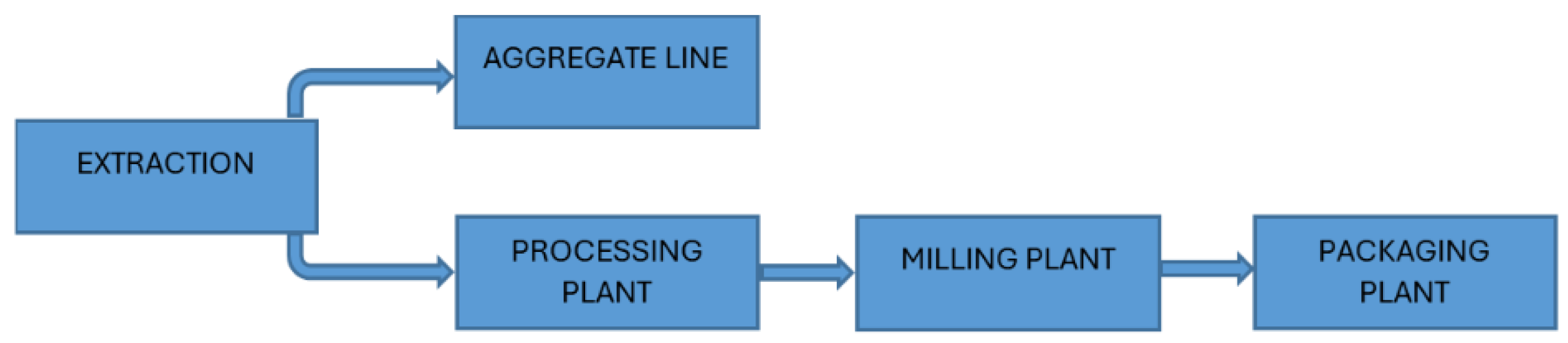
Kopalnia Wapienia Czatkowice carries out a comprehensive process of limestone extraction and processing, which includes several key technological stages:
Mining Plant: Extraction and aggregate production;
Mineral Processing Department: Mechanical processing plant, limestone grinding plant, storage and loading unit, and milled product packaging station.
The entire production process is divided into individual stages, as illustrated in
Figure 1.
Depending on its chemical composition (e.g., lead, silica, or magnesium content), the raw material is routed either to the aggregate plant or to the processing plant. Limestone with increased silica content is used for the production of commercial aggregates, whereas raw material with lower silica content is processed into limestone flour, sands, and stones.
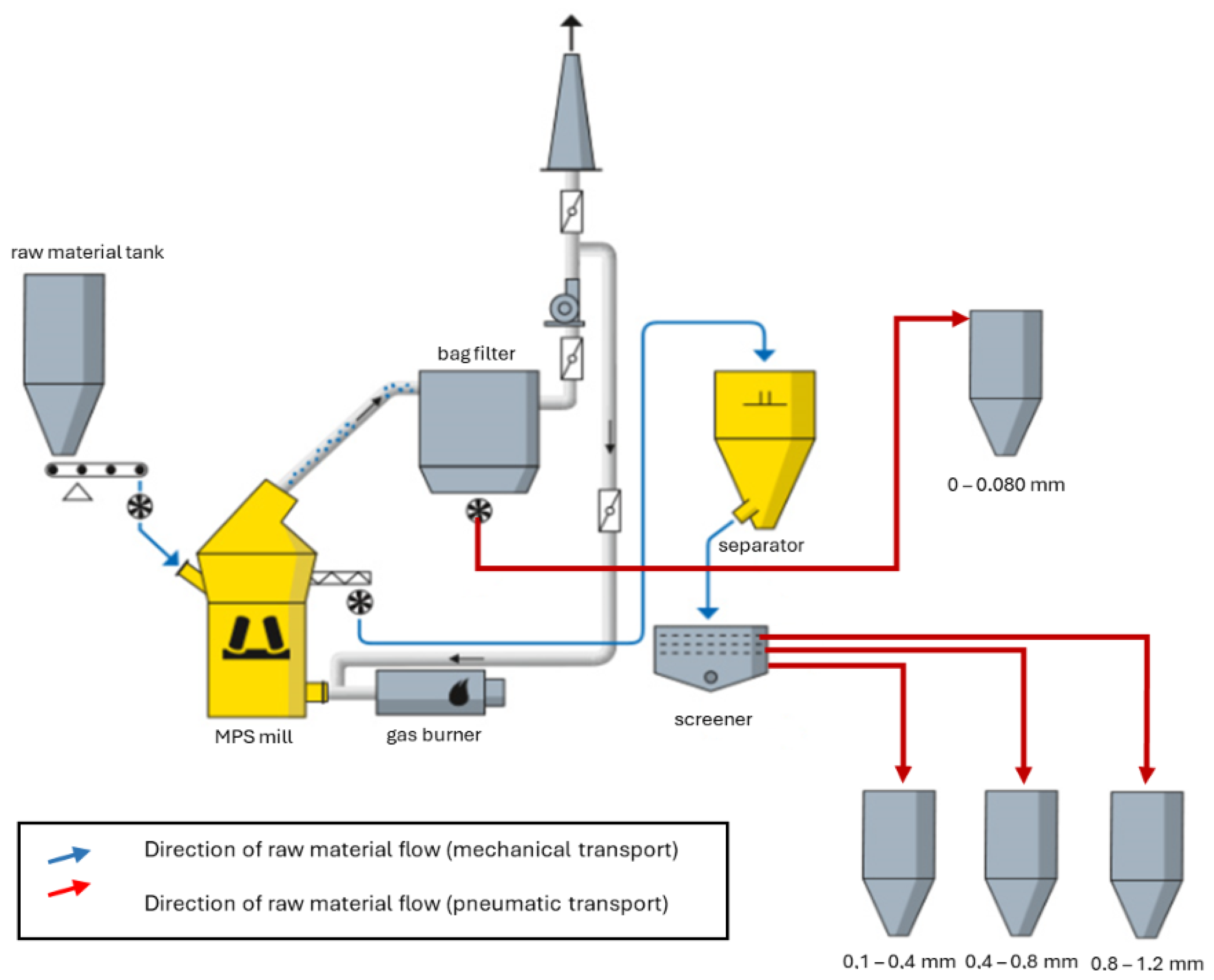
Grinding Plant: The technological grinding system, shown in
Figure 2, consists of two parallel twin processing lines featuring high complexity and technological advancement.
Figure 2.
Simplified flow diagram of the grinding process at KW Czatkowice.
Figure 2.
Simplified flow diagram of the grinding process at KW Czatkowice.
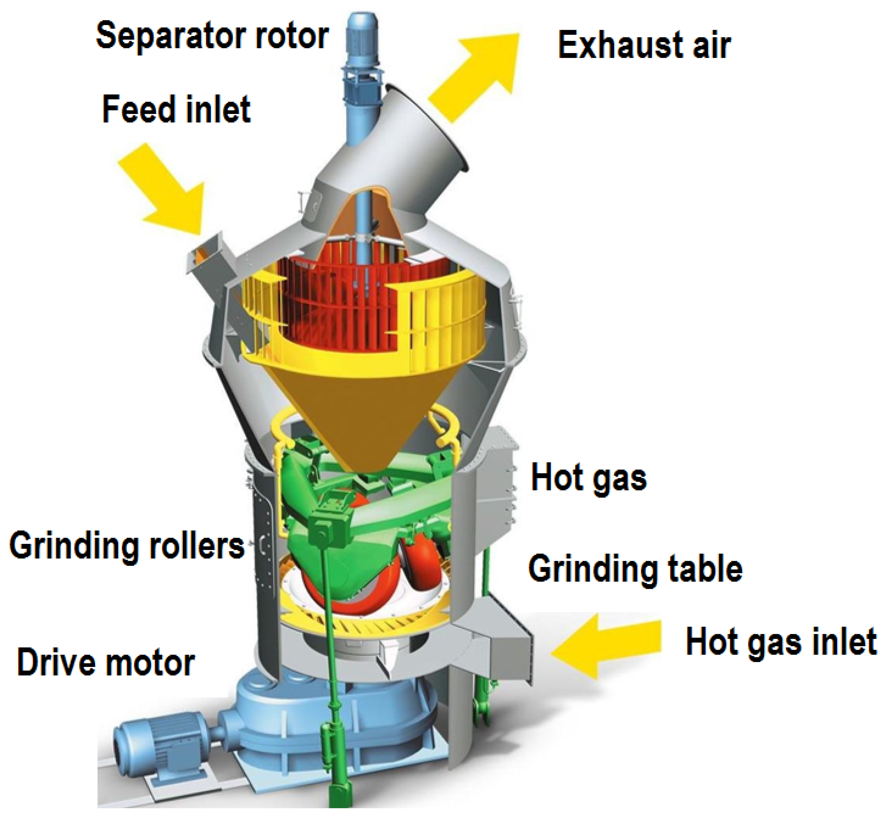
The main grinding equipment is a roller mill manufactured by the German company GEBR: PFEIFFER (Kaiserslautern, Germany) (
Figure 3), with a throughput of up to 80 tons per hour.
Material enters the mill through buffer tanks, from which it is transported to the mill by dosing scales. The raw material falls onto a rotating grinding table and is crushed between rollers, resulting in grain sizes down to 4 mm. The grinding process is tightly integrated with drying—performed using a gas burner located at the mill inlet, which heats the air to approximately 250 °C.
The ground particles are then carried by an airstream generated by the process fan. A separator with a rotating rotor classifies the particles into fine and coarse fractions. Fine particles are directed to a dedusting installation and transported to storage as limestone flour with a grain size of 0.045–0.080 mm, while coarser particles (>0.08 mm) are sent back for further grinding or stored.
The cleaned air from the filter is directed to the mill fan, which discharges it through the chimney and returns it to the mill inlet as part of a closed-loop system.
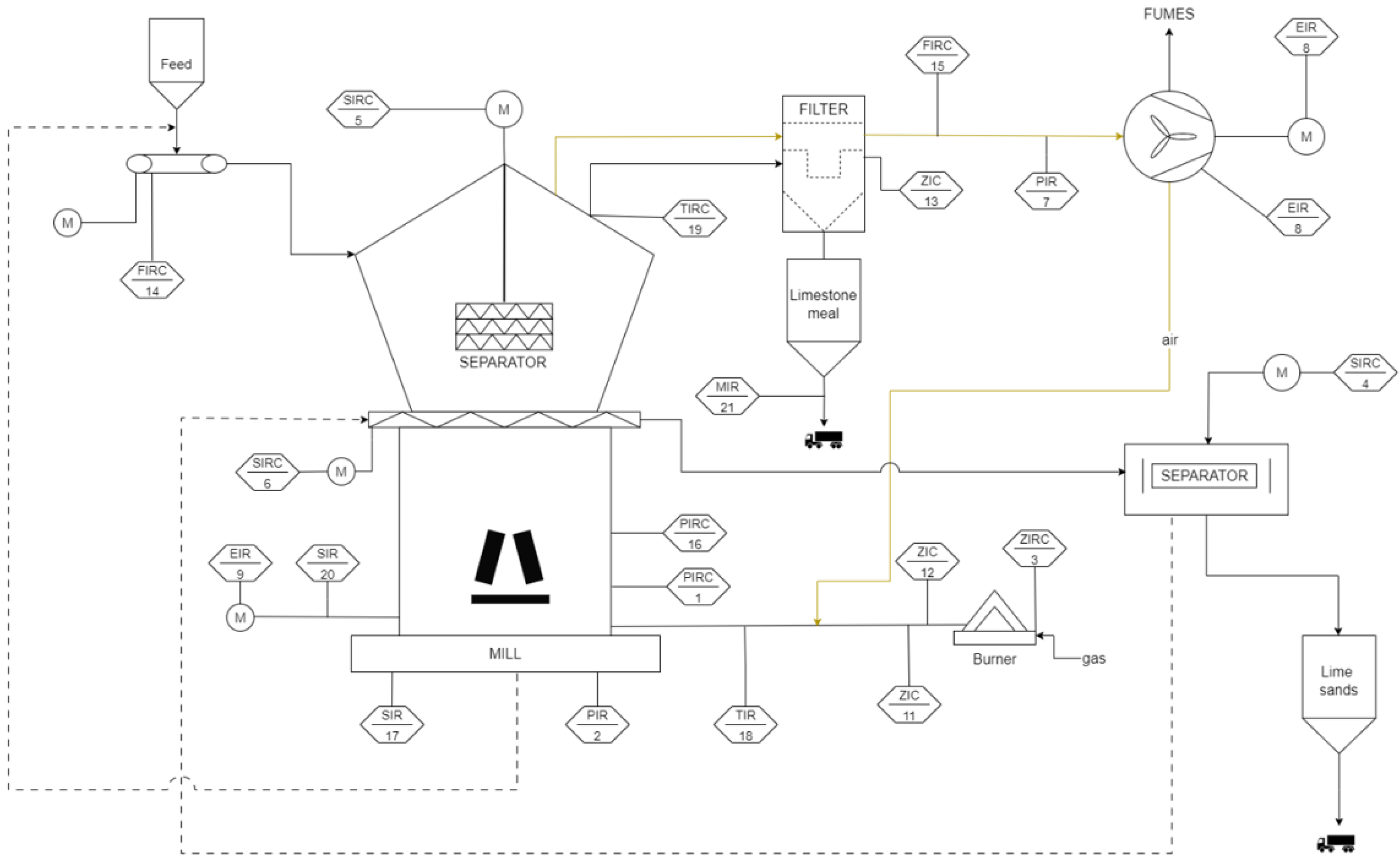
The production line is fully automated, and the entire technological setup is equipped with measurement and control instrumentation. A simplified diagram of the grinding line with key measurement points is shown in
Figure 4.
The analyzed system records over 3500 variables, enabling extensive process analysis. Process control relies heavily on operator experience, and the system is designed with redundancy (e.g., two clustered application servers, duplicated Ethernet connections, etc.) to ensure production continuity even in the event of component failure.
4. Cost Analysis
In order to identify the process responsible for generating the highest unit cost, a detailed cost analysis was carried out across all stages of raw material extraction and processing. Although operational costs vary, they must provide essential information for effective production management and informed business decision-making.
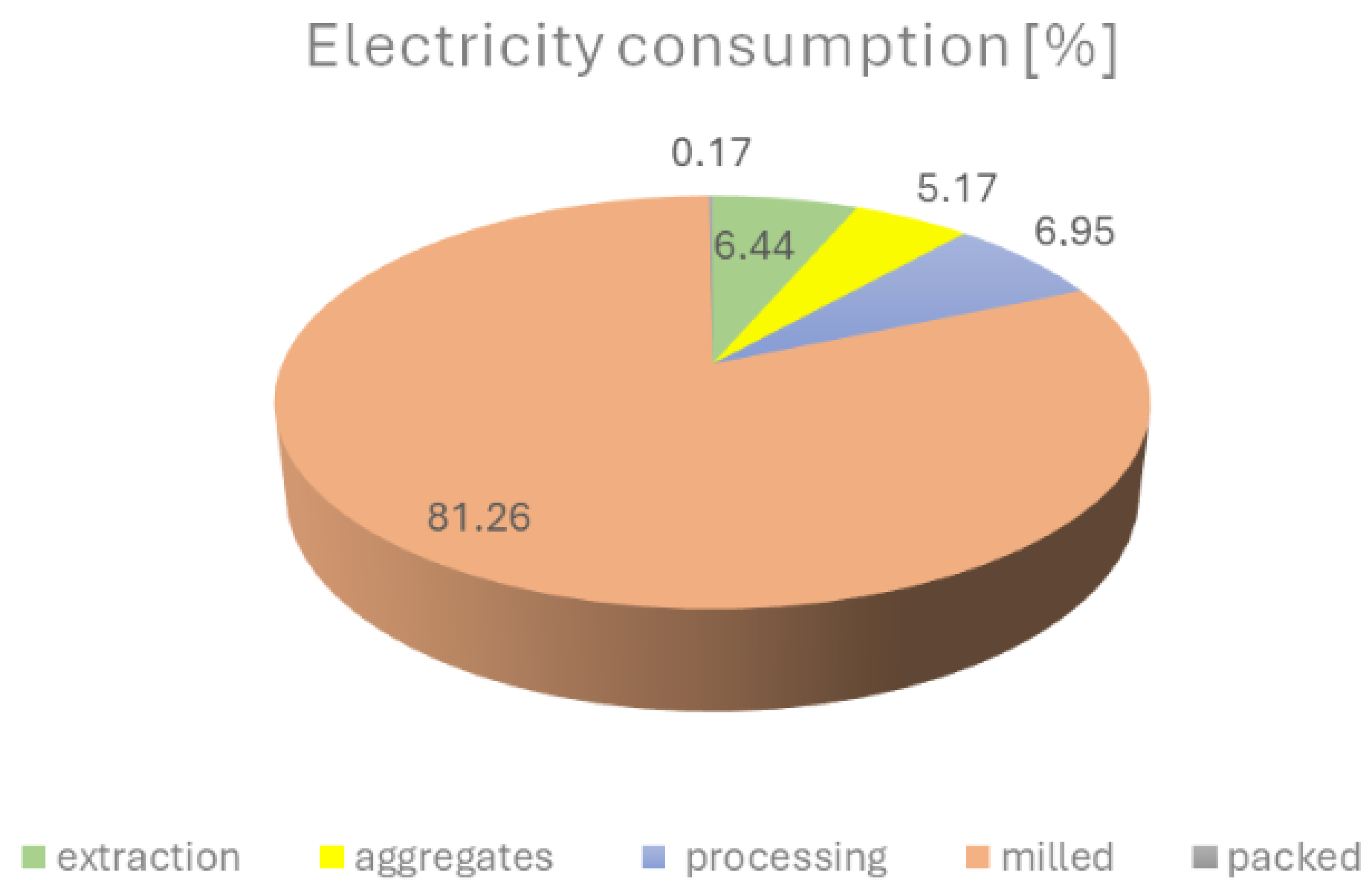
One of the key areas forming the foundation for process optimisation is the cost of utility consumption, particularly electricity and gas, which can be actively controlled. The analysis revealed that the grinding process is characterized by the highest electricity consumption (see
Figure 5). Moreover, it is the only stage of production that uses gas, which is necessary for product drying. Additionally, this process involves the largest number of machines and equipment in the entire technological cycle. For these reasons, it was identified as a key area for conducting factorial experiments and implementing optimisation measures.
5. Evaluation Indicators and Process Parameters
To improve the efficiency of the limestone grinding and classification circuit, it is essential to develop robust mathematical models supported by quantitative evaluation indicators. Considering both economic and technological criteria, two key energy indicators were formulated to assess the performance of the system.
The first of these indicators is the specific electric energy consumption (
S), which quantifies the ratio between the total power consumed by the main drive units—namely, the mill and the main fan—and the mass flow rate of the limestone (
1). It is defined as follows:
To further enhance the precision of energy performance evaluation, a second indicator (
W) was introduced (
2). This modified index additionally incorporates the gas consumption of the mill, represented by the relative load of the gas burner:
where:
S: Specific electric energy consumption [kWh/Mg].
W: Modified energy consumption indicator accounting for burner load [kWh/Mg].
: Mill motor power consumption [kW].
: Main fan motor power consumption [kW].
: Limestone feed mass flow rate [Mg/h].
: Relative load of the gas burner [%].
The objective of process optimisation is to minimize both indicators, thereby reducing energy intensity while maintaining or improving technological performance.
The modelling of these indicators was based on real-time process data collected by the SCADA (Supervisory Control and Data Acquisition) system implemented in the KW Czatkowice grinding plant.
Measured Process Parameters
The key process variables recorded by the SCADA system were used to develop and validate the proposed energy indicators.
Table 1 summarizes the selected parameters and their respective notations and units.
6. Experimental Conditions
The data used to build the neural network models were collected from a factorial experiment conducted at the grinding plant of KW Czatkowice in November and December 2023, covering five work shifts. As part of the experiment, four key controllable parameters were selected:
Screw conveyor motor speed;
Temperature after the mill;
Airflow before the main fan;
Pressure drop across the mill.
Each parameter was tested at three different levels. Each experiment lasted for 3 h, with a 1-h stabilization period between tests to allow process parameters to settle. During the experiments, automatic control loops in the SCADA system were disabled, which made it possible to capture the boundary conditions of the process. Detailed experimental conditions are shown in
Table 2.
7. Optimisation of the Grinding Process Using Artificial Neural Networks
In modern manufacturing, the optimisation of machining processes is crucial for improving product quality, reducing costs, and increasing efficiency. Among these processes, grinding plays a key role in achieving high surface quality and dimensional accuracy. Traditional optimisation approaches often rely on empirical methods or simplified mathematical models, which may not fully capture the complexity of the process. ANNs offer a promising alternative, as they are capable of modelling nonlinear relationships between process parameters and quality outcomes based on experimental data. This section presents the development and validation of ANN-based models for predicting key evaluation indicators in the grinding process.
7.1. Design of a Predictive Model for Evaluation Indicators Using ANN
Regression models were developed based on the analysis of correlations between process data and quality evaluation indicators. However, system designers do not have direct control over these process variables. It was decided to create a predictive model for the evaluation indicators using variables that can be controlled, as presented in
Table 3.
7.1.1. Model Architecture
As an additional method for modelling the energy indicators, artificial neural networks were proposed. The developed model performs a regression task, producing a single continuous output representing the selected evaluation indicator [
66]. The model was implemented using the TensorFlow library and its high-level API, Keras [
67], and was designed with a fully connected, feedforward architecture.
The input to the model consisted of selected controllable process variables. The architecture is composed of the following layers:
7.1.2. Loss Function and Metrics
The mean squared error (MSE) was selected as the primary loss function due to its convexity and strong statistical grounding in Gaussian likelihood estimation. It penalizes large deviations more heavily, leading to improved accuracy in most regression tasks:
To complement MSE, the mean absolute error (MAE) was also computed:
While MAE treats all errors equally and is robust to outliers, MSE emphasizes larger discrepancies. Together, they provide a comprehensive view of both typical and extreme prediction errors. Additional metrics reported include the root mean squared error (RMSE) and coefficient of determination (), which quantify overall predictive performance.
7.1.3. Model Training
The model was compiled using the Adam optimiser [
68], which adaptively adjusts learning rates for each parameter using estimates of first- and second-order gradient moments. This optimiser combines the strengths of AdaGrad and RMSProp [
69], making it well-suited for complex, non-convex optimisation tasks such as neural network training.
An exponentially decaying learning rate schedule was employed, beginning at an initial learning rate of 0.001. Prior to training, each dataset was randomly split into training and test subsets, with 20% of the samples reserved for testing. The remaining 80% of the data was used to train the model, within which an additional 20% was internally allocated for validation during training.
The training process was carried out over 1000 epochs with a batch size of 64. To prevent overfitting and improve model generalization, the following callbacks were employed:
ModelCheckpoint—Saves the model with the lowest validation loss.
EarlyStopping—Stops training if no improvement in validation loss is observed for 10 consecutive epochs.
TensorBoard—Enables the real-time visualization and diagnostics of training metrics.
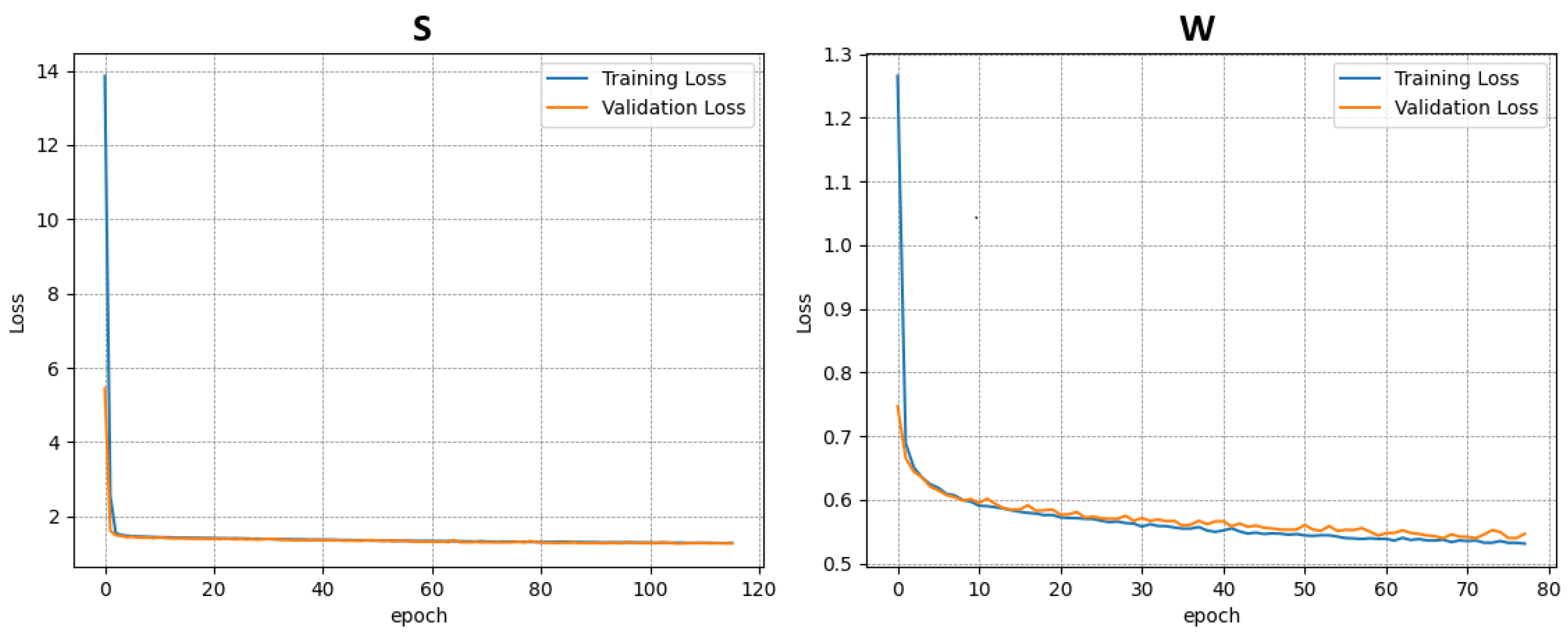
After training, model performance was evaluated on the separate test set using the metrics described above. Training outcomes were visualized using the following:
Training and validation loss curves across epochs.
Scatter plots comparing actual vs. predicted values across key features.
Boxplots of the distributions of actual and predicted indicator values.
All results were saved for further analysis and model benchmarking.
7.2. Design of a Hybrid Ensemble for Evaluation Indicators
Single-model regressors often struggle to capture both the highly nonlinear behaviour of the gas–solid mixture and the piece-wise linearities introduced by mechanical constraints (e.g., v-belts, variable-speed drives). We therefore combine two learners with complementary inductive biases in a heterogeneous ensemble, allowing the downstream optimiser to exploit a smoother and more reliable surrogate response surface.
All predictors are restricted to the four adjustable variables listed in
Table 3. This guarantees that any optimal operating point proposed by the model remains physically achievable by the plant PLC. Historical values outside the editable range are discarded, preventing the learners from extrapolating into unsafe regions.
7.2.1. Base Learners
Two complementary base learners were selected for the ensemble model: a multilayer perceptron (MLP) and a gradient-boosted tree model (XGB). Their key characteristics and hyper-parameters are summarized in
Table 4.
7.2.2. Data Preparation
A historical log is first filtered for steady-state intervals. Records are split chronologically into 80% training and 20% testing segments to mimic forward prediction. Continuous inputs are standardised, while the target undergoes the log-transform , yielding near-Gaussian residuals and stabilised variance; the inverse map is applied before reporting errors in physical units.
7.2.3. Ensemble Construction
Let
and
denote the base predictions. A convex combination yields the final estimate:
Weights are fixed at because cross-validation showed that (i) either the learner alone dominates only in the isolated corners of the input domain and (ii) performance variance grows when the ensemble is tuned on small validation folds.
Interpretability Note
While the arithmetic mean sacrifices the global feature-importance scores produced by XGBoost, local Shapley values can still be computed for each constituent and aggregated, allowing engineers to trace counter-intuitive recommendations back to thermodynamic effects (MLP) or to dominant threshold rules (XGB).
7.2.4. Training and Evaluation
The MLP is trained for 1000 epochs (
EarlyStopping patience = 20); the XGB halts automatically when the validation MAE fails to improve for 50 rounds. The evaluation on the hold-out set uses
,
, and
:
7.2.5. Evaluation of the Predictive Model for Indicators
To evaluate the generalization capability of the neural network models, training and testing were conducted using four different datasets derived from the limestone grinding and classification system. These datasets, collected during various operational periods and experimental campaigns, were extracted from the SCADA system and preprocessed to retain 26 relevant process variables—primarily those that are controllable.
An overview of the datasets used is provided below:
- (A)
July–December 2022—Consists of 7440 samples and 26 variables, representing routine operational data from the second half of 2022.
- (B)
Industrial Experiments 2023—Contains 2226 samples and 26 variables. This dataset was recorded during targeted industrial experiments conducted in 2023 to explore new process configurations.
- (C)
June–August 2023—Includes 4294 samples and 26 variables, capturing standard plant operations during the summer months of 2023.
- (D)
Combined Dataset—An aggregated dataset comprising all of the above, totalling 13,960 samples. It was constructed to develop a model capable of capturing more general patterns across varied operating conditions.
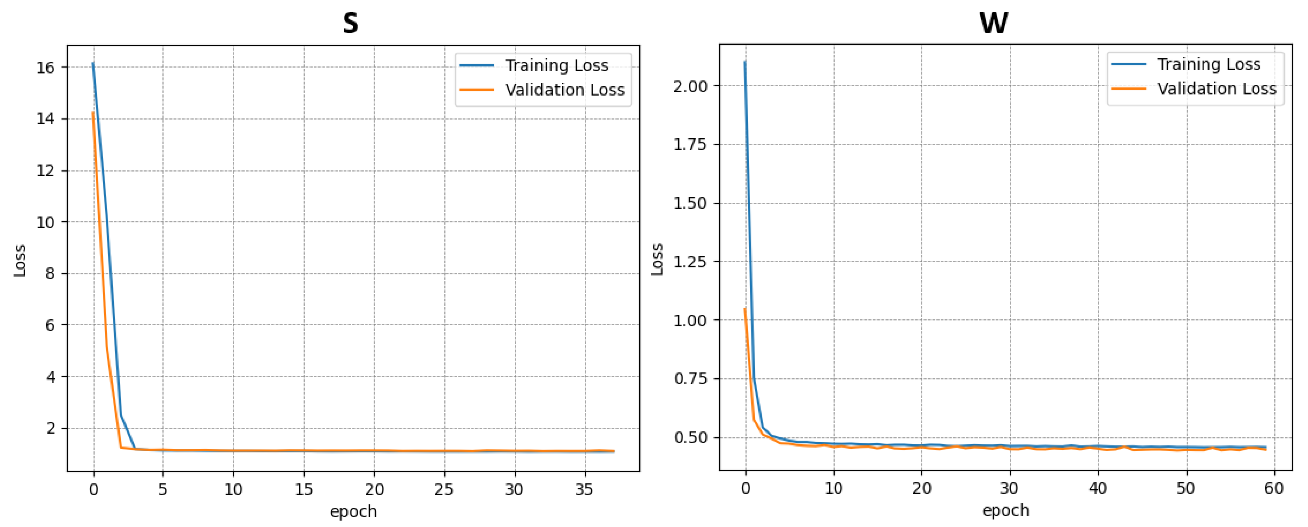
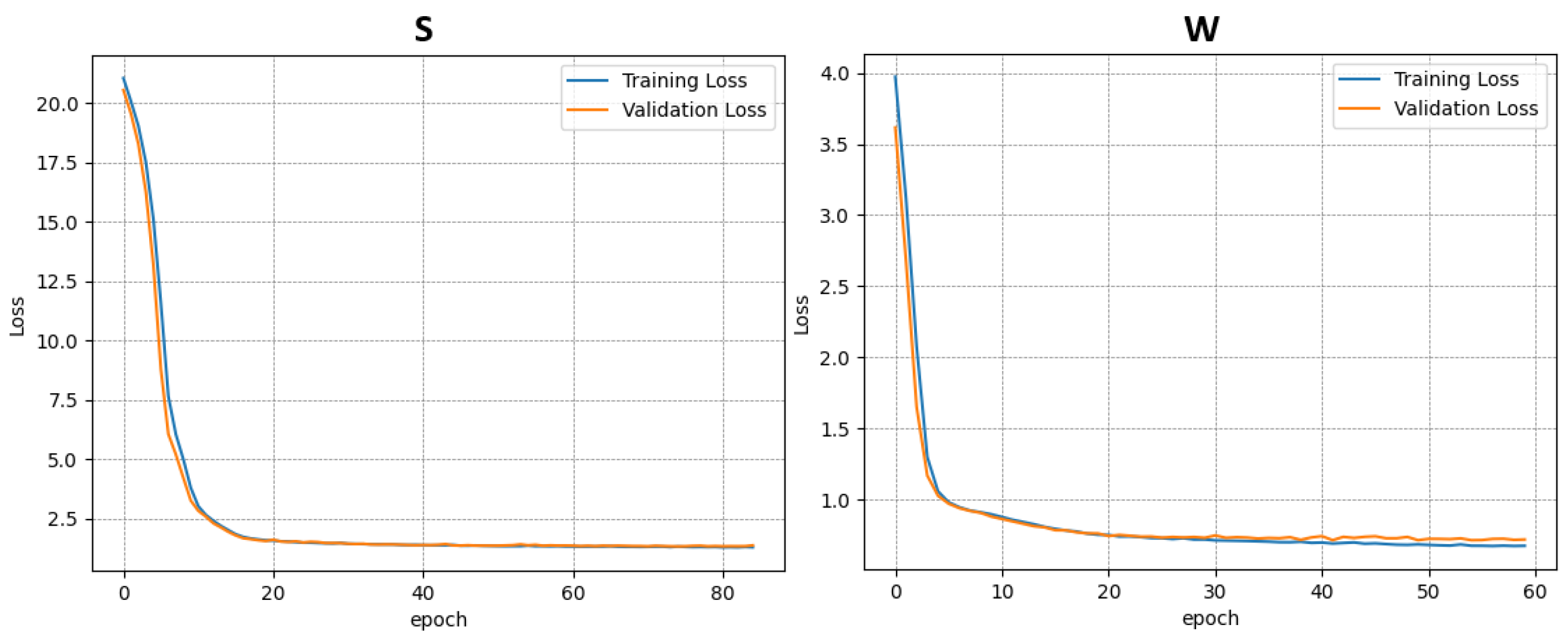
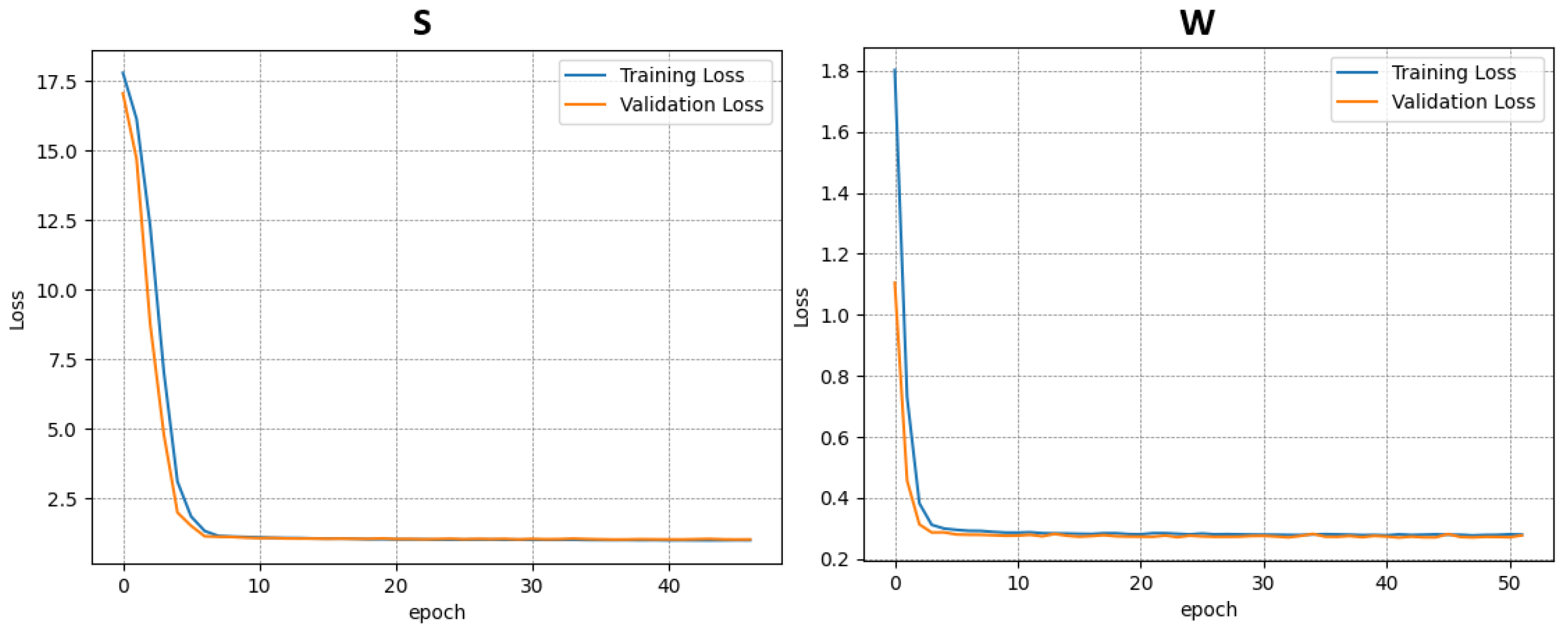
Each dataset was used independently to train a separate instance of the model. In total, four training procedures were performed—three on the individual datasets (A–C) and one on the combined dataset (D). The results of the training and validation phases for each case are presented in
Figure 6,
Figure 7,
Figure 8 and
Figure 9.
This approach allowed for the assessment of model performance under both specific and generalized data conditions, facilitating comparisons between specialized and broadly trained models.
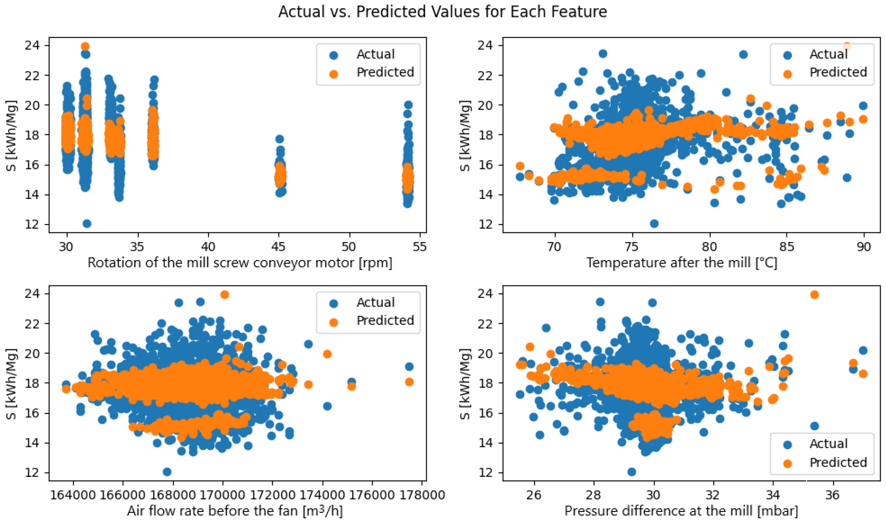
After the training process, each model was tested on the individual datasets used during the training phase. The model, which is a function of four variables (the controlled parameters), was represented using four plots that show the evaluation indicator as a function of the controlled parameters. For each comparison between the actual and predicted values, the distribution of these values was presented, providing a more detailed insight into the performance quality of the models (
Figure 10,
Figure 11 and
Figure 12).
Based on the comparison between actual (blue) and predicted (orange) S-index values for dataset A (
Figure 10), several patterns emerge. First, the model consistently “compresses” its prediction range: While the true S varies from about 13 to 24 kWh/Mg, the forecasts lie mainly between 15 and 20 kWh/Mg, indicating an underestimation of the highest values and an overestimation of the lowest. Second, different process features reveal distinct error patterns: At very low and very high mill-screw speeds, the model fails to capture the steep rise or fall in energy use; for temperatures after milling, the slope of the predicted trend is noticeably shallower than in the real data; with airflow, predictions form a narrow “corridor” while the true values spread out at extreme flows; for pressure drop, the model hits the central region accurately but underestimates S at high drops and overestimates it at low drops. Moreover, the scatter of residuals varies by feature: For temperature, the error band remains relatively uniform, whereas for pressure drop, it widens at the axis extremes. In practice, this means the model predicts the distribution center well but loses reliability near the parameter boundaries. To improve performance, one should extend factorial experiments to include boundary settings, introduce nonlinear transformations of the input variables (e.g., squares or interaction terms), and consider uncertainty quantification techniques to flag high-risk operating regions.
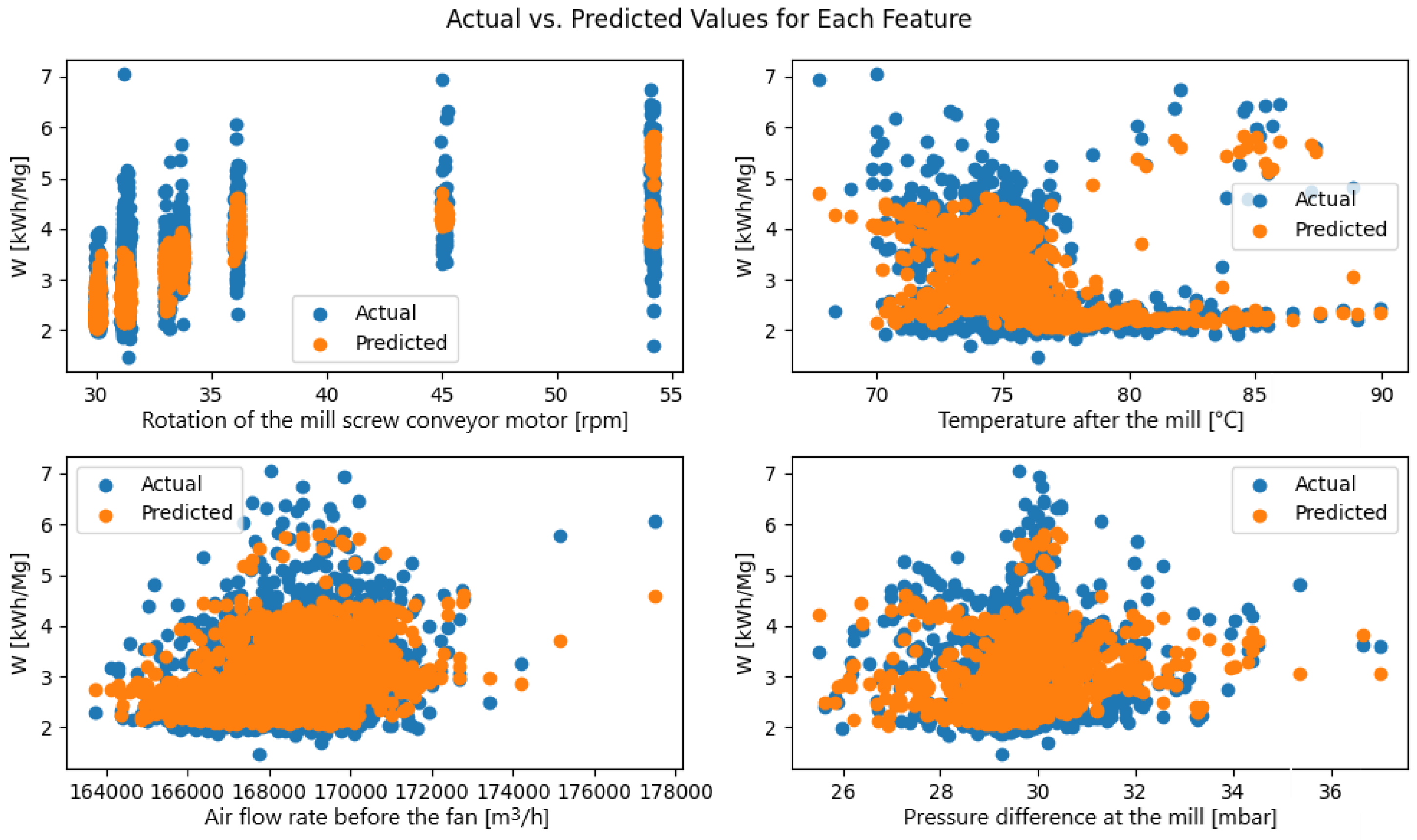
The analysis of the plots in
Figure 11 comparing actual and predicted
W-index values for dataset A as a function of the four controllable variables shows that the model performs better here than it does for the S-index, although it still compresses the extremes slightly. The true W ranges roughly from 1.5 to 7 kWh Mg
−1, whereas the forecasts are concentrated mainly between 2 and 5 kWh Mg
−1, so the highest consumptions are somewhat underestimated and the lowest ones are overestimated. At very low and very high screw-conveyor speeds, the model underpredicts W, yet in the central speed band (≈32–36 rpm), the two point clouds almost coincide. With respect to the temperature after the mill, a bimodal pattern emerges: For 70–76 °C, the actual and predicted values overlap closely, while above 80 °C, the forecasts clustering around 3 kWh Mg
−1 fail to capture the real increase in energy use that reaches 6–7 kWh Mg
−1. Across the range of air-flow rates before the fan the model reproduces the lower and middle regions well, and only at the highest flows (beyond about 175,000 m
3h
−1) does a mild underestimation appear. For the pressure drop across the mill, the predictions almost trace the envelope of the actual data, with larger errors occurring only at the extremes—below 26 mbar and above 34 mbar.
Error statistics confirm the visual impression. For dataset A, the mean absolute error and coefficient of determination are roughly 0.28 kWh Mg−1 and 0.25 for W versus about 0.98 kWh Mg−1 and 0.19 for S. In other words, the network captures the variability of the W-index far more accurately—especially in the middle operating range—whereas its predictions for S are more strongly flattened and deviate more from observations, particularly in the extreme regions.
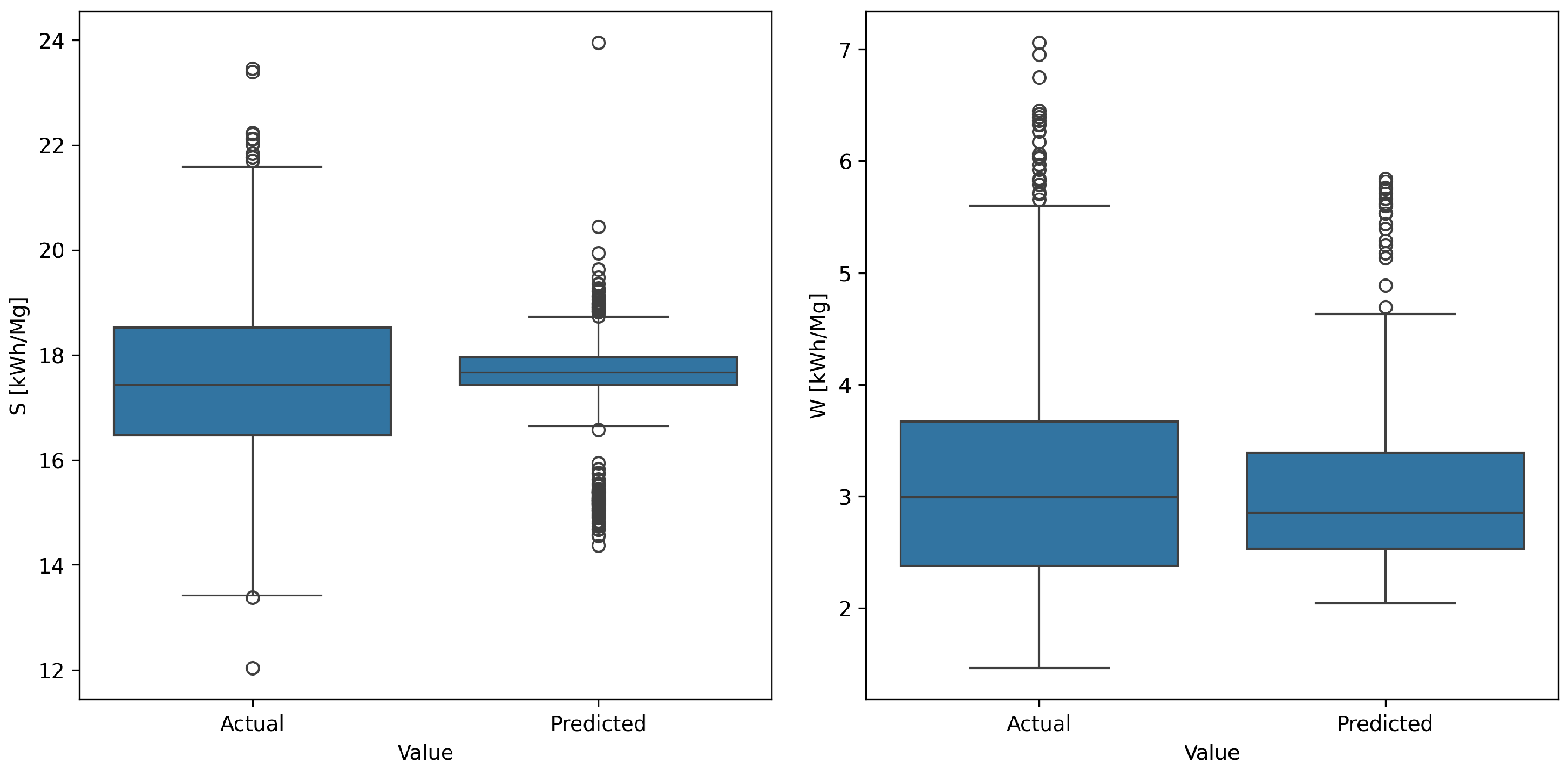
Figure 12 presents the empirical and predicted distributions of both indices using box-and-whisker diagrams. For the S-index (left panel), the centres of the two boxes—median and inter-quartile range—almost coincide, indicating that the model reproduces the process mean quite well. Nevertheless, the forecasted distribution is markedly narrower: Its inter-quartile span is roughly half that of the real data, and the extreme observations (below about 14 kWh Mg
−1 and above 22 kWh Mg
−1) are virtually absent. The model therefore pulls the tails toward the mean, confirming the previously noted tendency to compress variance.
The pattern is similar, though less pronounced, for the W-index (right panel). The predicted median, around 2.8 kWh Mg−1, lies very close to the empirical median, and the model’s box covers almost the same central range as the data. Differences re-emerge at the extremes: Actual values extend down to roughly 1.8 kWh Mg−1 and up to nearly 7 kWh Mg−1, whereas the model seldom drops below 2.3 kWh Mg−1 or exceeds 4.5 kWh Mg−1.
In summary, the boxplots show good agreement in central tendency for both indices but a systematic flattening of the tails. The surrogate is therefore reliable for predicting typical energy consumption, yet it remains overly conservative in the most expensive or risky operating states. Practically, this means that the forecasts are useful for day-to-day optimisation, but when analysing boundary conditions—such as full-load operation or emergency flow reductions—additional outlier-detection or safety margins are advisable.
The distributions of actual and predicted values suggest that the models perform better in predicting the
W indicator across all datasets, as the actual values and predictions overlap significantly. For the
S indicator, the model trained on the dataset from the industrial experiment performs the best. However, the prediction distributions of all models fall within the range of actual values, which is a positive signal, indicating prediction accuracy. The model’s metrics are presented in
Table 5.
A comparison of results (
Table 5) confirms that the hybrid ensemble model consistently outperforms the standalone ANN in terms of predictive accuracy across both energy indicators (S and W). The ensemble yields lower MAE, MSE, and RMSE values in most datasets, indicating a better fit and more reliable generalization capability. This advantage is particularly evident for the W indicator, where the ensemble achieves substantially higher
values (up to 0.54 for dataset A) compared to the ANN. The superior performance of the ensemble stems from the complementary strengths of the MLP and XGBoost components, enabling the model to capture both smooth nonlinearities and sharp threshold effects inherent in the grinding process.
8. Optimisation of the Neural Network Model
Similarly to the training process of the ANN model, the optimisation of the black-box type function was carried out for the same four cases. In the previous case, all variables used to construct the indicators
S and
W were considered. This approach may be partially valid, as these indicators may indirectly depend on the controlled variables. For example, vibrations could be influenced by the operation of the mill, but they may also depend on the composition and granularity of the crushed material. From a control perspective, vibrations represent a disturbance in the system and are only partially correlated with control inputs. Therefore, it was decided to determine the local minima of the energy indicators considering only the controlled variables (
Table 3): that is, the parameters over which direct control can be exerted. Two separate mechanisms were used for optimisation: Bayesian optimisation and a genetic algorithm. These algorithms allowed, on the one hand, the estimation of missing state variables (system states that were not directly measured) and, on the other hand, the finding of local minima for the
S and
W indicators.
Bayesian Optimisation
Bayesian optimisation is a global optimisation strategy designed for problems where the objective function is expensive to evaluate, lacks an analytical form, and may be noisy [
70,
71]. It is particularly effective for optimising black-box functions such as those represented by deep neural networks. The goal is to find
subject to the following conditions:
f is a black-box function with unknown analytical form and gradients;
Evaluations of are computationally expensive;
Observation may be noisy.
Given these constraints, Bayesian optimisation is well-suited for optimising data-driven models like neural networks used in this work. The method constructs a surrogate model of the objective function using a Gaussian process (GP), which is updated iteratively based on observed data. The algorithm proceeds as follows [
72]:
- 1.
At iteration t, a GP model, is fit to the observations for .
- 2.
A computationally inexpensive acquisition function is optimised to select the next point for evaluation: .
- 3.
The objective function is evaluated at to obtain .
The acquisition function balances exploration and exploitation. In this work, the algorithm probabilistically selected among several acquisition strategies using the gp_hedge heuristic:
Expected Improvement (EI): ;
Lower Confidence Bound (LCB): ;
Probability of Improvement (PI): .
Here, is the best observed value to date, and and are the GP posterior mean and standard deviation, respectively.
In this study, Bayesian optimisation was employed to identify the optimal setpoints of controllable process parameters that minimize the predicted values of the energy indicators W and S. The optimisation was implemented using the gp_minimize function from the scikit-optimize library, which applies Gaussian process regression to iteratively refine the search space.
The objective functions were constructed using previously trained neural network models:
Here, represents a vector of normalized controllable process variables.
The optimisation was performed independently for each indicator with the following configuration:
Total evaluations: 50.
Initial random samples: 10.
Acquisition strategy: gp_hedge.
Random seed: 42 (to ensure reproducibility).
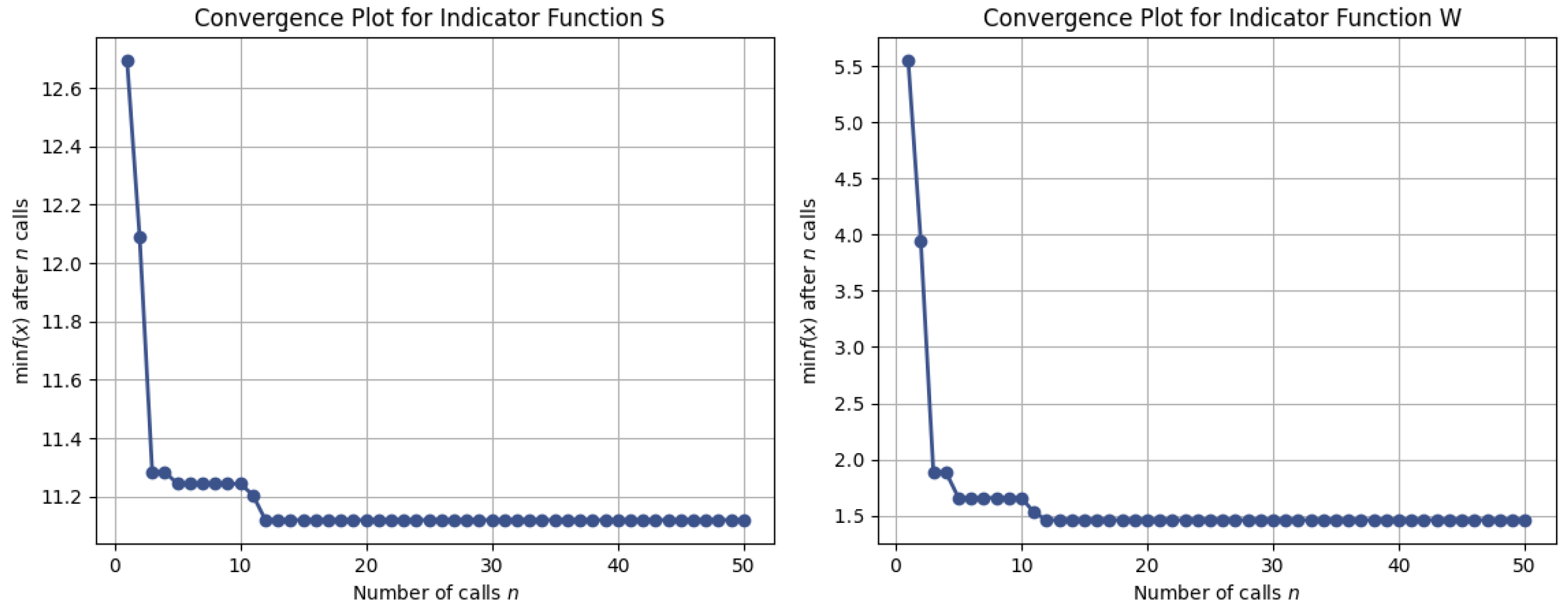
At each iteration, the surrogate GP model was updated with the latest data, and the next candidate point was selected by maximizing the acquisition function. This iterative procedure converged toward the minimum of the surrogate model, yielding the following:
The convergence of the optimisation process was visualized using convergence plots, depicting the evolution of the best observed function value over iterations.
Figure 13 illustrates the convergence behavior of the Bayesian optimisation process for both indicators. The plots demonstrate that the optimization algorithm rapidly approaches near-optimal values within the first 10–15 evaluations and stabilizes thereafter. This confirms that the ensemble-based surrogate models provide not only improved predictive accuracy (
Table 6,
Table 7,
Table 8 and
Table 9) but also reliable guidance for downstream optimisation tasks, ensuring effective search for energy-efficient operating conditions.
This approach offers an efficient, data-driven methodology for determining optimal operating conditions without relying on the explicit physical modelling of the process.
9. Optimisation Using Genetic Algorithms
Genetic algorithms (GAs) are a class of population-based metaheuristic optimisation techniques inspired by evolutionary mechanisms such as natural selection, crossover, and mutation [
73]. These algorithms are particularly effective for solving black-box optimisation problems where the objective function is nonlinear, non-convex, multimodal, or expensive to evaluate [
74,
75].
In the context of this study, GA was applied to optimise controllable process parameters with respect to the predictive energy efficiency indicators W and S. Each solution is represented as a chromosome—a real-valued vector corresponding to the input variables of the model. The optimisation goal was to minimize the value of each indicator as predicted by the trained neural networks. Accordingly, the fitness functions were defined as follows:
Here, is a vector of normalized controllable process variables.
The genetic algorithm follows the general steps outlined below:
- 1.
Population Initialization: A population of candidate solutions (chromosomes) is initialized randomly within defined parameter bounds.
- 2.
Fitness Evaluation: Each chromosome is evaluated using the fitness function, assigning a fitness score based on the predicted indicator value.
- 3.
Selection: The most fit chromosomes are selected for reproduction using a rank-based selection mechanism.
- 4.
Crossover: Selected parent chromosomes are recombined to generate offspring, introducing genetic diversity into the population.
- 5.
Mutation: Offspring undergo random mutations at a low probability to avoid premature convergence and encourage exploration.
- 6.
Replacement: Offspring replace part of the existing population to form the next generation.
- 7.
Termination: The algorithm continues iterating until a predefined number of generations is reached or convergence criteria are satisfied.
In this study, the implementation was carried out using the pygad library with the following configuration:
Number of generations: 100.
Population size: 100 individuals.
Number of genes: Equal to the number of controllable parameters.
Parent selection method: Rank selection.
Number of parents selected per generation: 10.
Number of elite (retained) parents: 2.
Mutation probability: 10%.
Gene space: Bounded ranges defined for each control variable.
Two independent optimisation runs were conducted—one for minimizing indicator W and one for S. Over 100 generations, the population evolved toward optimal solutions using crossover, mutation, and selection mechanisms.
The final output of the algorithm includes the best-performing solution (chromosome) and the corresponding minimum value of the indicator:
at ;
at .
This evolutionary strategy complements Bayesian optimisation by enabling a stochastic, global search of the parameter space. Its robustness to local minima and independence from gradient information make it particularly well-suited for optimising data-driven industrial models. The final optimisation results are summarized in
Table 10,
Table 11,
Table 12 and
Table 13.
It is worth noting that both optimisation methods identify very similar energy minima for the S and W indicators. Both genetic algorithms and Bayesian optimisation effectively find system operating parameters that result in significantly lower energy consumption compared to the previously used heuristic settings.
One striking observation is that despite the distinct control values selected from the assumed range of parameter variability, both methods achieve very similar indicator values. This suggests that the entire state space contains multiple local minima. Therefore, it is reasonable to use two different optimisation algorithms. However, genetic algorithms may discover alternative local minima, which could be more advantageous for the enterprise from an operational or production management perspective.
10. Results
This analysis focused on two key aspects regarding the use of neural networks for optimising mill operations:
In the first case, neural networks were used to identify the model’s hyperplane, which allowed for determining the quality indicators even when some signals were unobservable. This means that the developed neural network model can estimate the values of S and W even in the event of sensor failure. On the other hand, when all signals are available, the mechanism can predict the indicator values for different parameter settings without requiring additional experimentation. The practical application of this methodology can serve comparative purposes, avoiding costly experiments. The system operator can obtain a set of indicator values for the current operating state. By adjusting individual parameters and processing them through the proposed neural network, the operator can determine whether the indicators improve. In this way, an optimal set of parameters can be determined and implemented in the actual system.
The second part of the analysis employed two different approaches to optimising black-box functions, aiming to optimize the mill’s operating parameters for four different cases (datasets A–D). Both Bayesian optimisation and genetic algorithms successfully identified operating settings that minimize energy indicators S and W. The results demonstrate that Bayesian optimisation achieved slightly better energy savings in several cases, although genetic algorithms also found comparable settings.
Importantly, the ensemble model developed in this study exhibited significantly better fit quality compared to standalone artificial neural networks, as confirmed by lower error metrics (MAE, MSE, and RMSE) and higher values across multiple datasets. Despite the improved predictive accuracy of the ensemble model, the optimisation results obtained using this model were comparable to those achieved with the standalone ANN models. This indicates that the ensemble model not only provides more accurate predictions but also delivers consistent and reliable guidance for downstream optimisation processes, ensuring practical applicability in industrial settings.
A comparison of energy savings before and after optimisation is shown in
Table 14.
11. Conclusions
This study demonstrated the development and validation of advanced data-driven models for predicting and optimising the energy performance of industrial limestone grinding. By combining ANN and a hybrid ensemble model incorporating MLP and XGBoost, we successfully established a predictive framework that performs reasonably well.
The proposed ensemble model exhibited superior predictive accuracy compared to standalone ANN, as confirmed by lower MAE, MSE, and RMSE values across multiple datasets and higher R2 coefficients, particularly for the W energy indicator. These improvements stem from the ensemble’s ability to jointly capture smooth nonlinear interactions and piecewise linearities characteristic of the grinding process.
Importantly, despite the enhanced predictive capability, the optimisation results obtained using the ensemble-based surrogate models are comparable to those generated by the standalone ANN. Both Bayesian and genetic optimization approaches, when applied to the ensemble models, identified operational settings that deliver similar energy savings, confirming the consistency and reliability of the optimised solutions. The ensemble model, therefore, provides a more accurate yet equally practical tool for real-world energy optimisation tasks.
The findings of this research validate the robustness and industrial relevance of AI-enhanced surrogate modelling in mineral grinding processes. The proposed methodology offers a data-supported basis for optimising energy consumption while maintaining operational flexibility and process stability. Future work will focus on integrating these models into real-time control architectures and extending the approach to other comminution technologies.
Limitations: Although the training log contained nearly 14,000 steady-state records, only nine factorial test runs were available to probe the extreme corners of the operating envelope. All data originated from a single limestone line in one plant, lithological changes or a different mill design could therefore shift the response surface and reduce model accuracy. In addition, the validation presented here is strictly open-loop: the recommended set points were compared with historical measurements offline, so potential feedback effects such as recycle loads or product-quality drift were not captured.
Future work: To move from offline feasibility to full industrial deployment, we plan to (i) embed the ensemble surrogate and Bayesian optimiser in the plant’s SCADA system with automated set-point, write-back, and rule-based failsafes; (ii) run a multi-month closed-loop trial to quantify long-term savings under variable ore hardness and ambient conditions; (iii) transfer the workflow to other comminution technologies such as ball mills and HPGRs; and (iv) investigate hybrid physics-informed networks that could reduce the amount of plant data required for re-training. Parallel studies will examine the economic impact of energy savings on the cost-per-tonne of product and the associated reduction in CO2 emissions. By addressing these points, we aim to establish a broadly applicable, field-proven toolkit for energy-aware optimisation across the mineral-processing sector.


 ,
, 
