Modeling Population Dynamics and Assessing Ecological Impacts of Lampreys via Sex Ratio Regulation

Abstract

Regulating lamprey populations is crucial for maintaining ecological equilibrium. However, the unique sex determination process of lampreys is constrained by multiple factors, complicating intuitive analysis of population dynamics and their impact on the natural environment. This study employed a two-species competition mechanism to elucidate the factors influencing sex ratios and their mechanistic effects on lamprey population size. Using the Lotka–Volterra equations, we investigated how sex ratios affect trophic levels both upstream and downstream of lampreys in the food web. A logistic population growth model was applied to assess the impact of sex ratio variations on symbiotic parasitic species, while the Analytic Hierarchy Process (AHP) was utilized to explore the dynamic relationship between sex ratio changes and ecosystem stability. To validate model efficacy, we manipulated temperature and food availability under controlled disturbance conditions, analyzing temporal variations in lamprey population size across different disturbance intensities to evaluate model sensitivity. The findings indicate that the variable sex ratio’s benefit is in facilitating the lampreys’ population’s enhanced adaptation to environmental shifts. The coexisting species exhibit a similar pattern of population alteration as the lampreys, albeit with a minor delay. A definitive link between the quantity of lampreys and the parasitic species is absent. A male ratio of 0.6 optimally contributes to the ecosystem’s equilibrium. Over time, the configuration of our model’s parameters proves to be sensible. This research provides robust theoretical support for developing scientific strategies to regulate lamprey populations.

1. Introduction

1.1. Background

Sea lampreys, resembling eels and feeding on blood, are widely distributed globally, as depicted in Figure 1. This species possesses a distinct mechanism for determining sex, governed by the larvae’s growth speed [1]. The growth rate of marine lampreys during the larval stage varies by the availability of food, which influences the sex ratio in adulthood. Adaptive sex ratio variation in nature is influenced by multiple factors and exerts significant effects at various biological scales, ranging from population-level dynamics to broader ecosystem processes. Consequently, examining how lampreys’ gender proportions correlate with their habitat’s resource availability is crucial for maintaining ecosystem stability over time.

We aim to create a comprehensive model to explore the interaction between the adaptive differences in the sex ratio of sea lampreys and ecological systems. The objective of this approach is to enhance the overall comprehension of sea lampreys’ biological characteristics and their ecological functions. Such a model not only helps to elucidate the underlying mechanisms of sea lamprey population dynamics but also offers valuable scientific insights for ecological conservation and management.

1.2. Review

The population of sea lampreys, a blood-feeding species that consumes the blood of other fish, plays a crucial role in maintaining the balance of the ecosystems they inhabit. As a result, the environmental effects of sea lampreys are garnering more focus from pertinent management bodies, making their population control a key concern in managing lake ecosystems. However, due to the inherent complexity of ecosystems and the need to account for the interplay of multiple factors, qualitative methods alone are insufficient for capturing the underlying dynamics.

Ecosystem modeling offers a promising alternative by incorporating both structural components and functional processes into a unified framework, enabling a more quantitative and systematic approach to ecological research. Scholars have explored ecosystem modeling across various dimensions, covering terrestrial [2], aquatic [3], and aerial [4] environments, and extending across domains such as agriculture [5], forestry [6], and fisheries [3]. Research has ranged from single-species studies to large-scale community and ecosystem modeling [7]. With increasing ecological challenges in recent years, such modeling approaches have become essential tools for both understanding and conserving ecosystems.

In terms of modeling techniques, several approaches have been developed: Christopher K. Wikle [4] employed hierarchical Bayesian models to incorporate parameter uncertainty and layered ecological structures, finding no significant time trend in house sparrow abundance. Miguel Lurgi et al. [8] used ecological network models to simulate how invasive species influence prey (e.g., rabbits) abundance, considering important feedback mechanisms. Hugo Fort [9] employed the linear generalized Lotka–Volterra model to demonstrate its predictive capability in multi-species systems.

However, these researchers frequently overlooked the ripple effects on the environment caused by changes in abundance. This paper addresses that gap by explicitly considering how population changes, especially those driven by sex ratio variation, can further affect ecosystem dynamics. While Zhen et al. [10] also employed the Lotka–Volterra framework to study total population and assess the influence of sex ratio changes, their model overlooked the life-history stages and developmental heterogeneity that characterize sea lamprey population structure. In this study, we incorporate a detailed life-cycle representation of sea lampreys, considering their distinct behavioral and ecological traits at different developmental stages. This integrated modeling approach offers a robust framework for simulating the ecological impact of adaptive sex ratio variation and provides deeper insights into sea lamprey population dynamics and their role within ecosystems.

1.3. Our Work

In this paper, we establish four mathematical models progressively and address four problems, which are shown in Figure 2.

Additionally, a summary of our key contributions is presented below:

(1)

Through the amalgamation of lampreys’ tripartite life cycle and their gender transition process, we developed a dual-species comparative framework grounded in differential equation methodologies. This model considers variations in population at various phases of the species’ growth and development, diverging from prior research.

(2)

Implementing the fourth-order Runge–Kutta technique guarantees the precision, steadiness, and intricacy of the outcomes. This facilitates a more effective computation of the outcomes derived from the dual-species competition model.

(3)

Employing a hierarchical analysis approach evaluates the impact of various elements on ecosystem stability, thereby enhancing the efficacy of the derived outcomes.

2. Assumptions and Symbols

To simplify the problem, we adopt the following basic assumptions, each of which is justified. Other assumptions based on different models will be listed in the following model-related sections.

Assumption 1:

Food availability is the main factor affecting the growth rate of sea lamprey larvae.

Justification: In nature, food availability directly affects the growth rate and survival of individuals. For many aquatic organisms, food availability is a key limiting factor in determining growth and development rates. Particularly for juvenile fish, adequate food supply can promote rapid growth and increase chances of survival, whereas food scarcity can limit growth rates and even lead to high mortality rates.

Assumption 2:

Variations in the sex ratio have a direct impact on the rate of reproduction and the size of the population.

Justification: Sex ratio is one of the key factors affecting the reproductive potential of a population. A balanced sex ratio ensures adequate reproductive opportunities, while a skewed sex ratio may reduce the reproductive success of a population, which in turn affects population size and growth rate.

Assumption 3:

Overlook the impact of disease spread and movement within and outside populations on the size of the population.

Justification: Although disease and migration have significant effects on population dynamics, ignoring these factors during the initial modeling phase simplifies the model and makes it easier to analyze and understand. This simplifying assumption allows the researcher to focus on food availability and sex ratio, two factors that more directly affect population growth.

Assumption 4:

Limit environmental carrying capacity.

Justification: Any ecosystem has a finite amount of resources, which limits the maximum sustainable size of populations living in that system. Environmental carrying capacity takes into account the limits of the resources available in an ecosystem and is an important predictor of population growth and stability.

Assumption 5:

Individuals at an identical developmental phase in a population are considered equal.

Justification: This assumption assumes that there are no significant genetic or phenotypic differences between individuals within a population, and thus that each individual is the same in terms of growth rate, survival rate, and so on. This simplification reduces the complexity of the model and is a practical approximation for large-scale population dynamics studies, although it may ignore inter-individual differences.

Assumption 6:

Once established, the sexes remain unchanged.

Justification: This reflects the biological reality of most vertebrates that the sex of an individual will not change once it is determined early in a life stage. This assumption simplifies the modeling of sex dynamics because it excludes the potential effects of sex transitions on population structure and dynamics.

The main notations used in this paper are listed in

Table 1. Notations used in this paper.

Symbol	Description
$\mathrm{K}$	Environmental capacity
$\mathrm{Ni}$	$\mathrm{The} i$-th lamprey population
${\delta }_i$	$\mathrm{Growth} \mathrm{rate} \mathrm{of} \mathrm{the} i$-th lamprey population
${\mu }_i$	$\mathrm{Mortality} \mathrm{rate} \mathrm{of} \mathrm{the} i$-th lamprey population
$f$	Total amount of food
$\mathsf{\eta }$	Environmental Resource Utilization

.

Additionally, sources of data used in the paper are websites such as the Great Lakes Fishery Commission and so on.

3. Resource-Dependent Sex Ratio Dynamics Model (RDSRD Model)

In this section, we analyze the advantages and disadvantages of adaptive sex ratio variation in sea lamprey populations under changing resource availability, based on a comprehensive modeling of their life cycle and supported by a population-level competition mechanism through simulation experiments.

3.1. Two-Species Competition Mechanism

This part will focus on creating a model for population competition, integrating the lampreys’ life cycle traits and gender determination processes.

Population expansion occurs in three distinct phases according to the life cycle

The life cycle of lampreys is a complex process divided into fourmain stages, each with its own unique physiological and ecological characteristics. These fourstages include the Hatching Stage, Larval Stage, Metamorphosis Stage, Adult Stage. The four-phase life cycle change is shown in Figure 3 below.

The Hatching Stage (HS) is the first stage of the life cycle of lampreys. Lamprey eggs are diminutive yet yield a substantial amount. On each occasion, their egg production ranges from 80,000 to 100,000. Typically, eggs are found clinging to sandy and gravelly surfaces. Soon after emerging, they transform into fry and progress to the larval phase.

The Larval Stage (LS) can last up to seven years or more, which is the longest stage of the lampreys’ life cycle [12]. During this period, larvae live on the bottom of freshwater streams, usually buried in silt or sand, forming U-shaped or slanted burrows.

The Metamorphosis Stage (MS) is relatively short and marks a rapid transition from larva to adult. At the end of this stage, individuals complete sex differentiation, which may be influenced by environmental conditions such as food availability.

The Adult Stage (AS) is the final stage of the lampreys’ life cycle and is shorter in duration relative to the larval stage. Mature lampreys evolve into predators, consuming tiny fish, invertebrates, and various animals. At maturity, lampreys return to freshwater streams to lay eggs and die shortly thereafter, completing their life cycle [12,13].

During the modeling process, the metamorphosis stage was ignored because it was in a transitional phase and had a relatively short duration. In conjunction with the stage characterization of sea lampreys, we divided the population growth model into three stages. The relationship between number changes in the three phases is shown in Figure 4 below. After the larva’s sex is determined, it transforms into an adult. The adult stage of lampreys is divided into male and female.

Consequently, the number of the lamprey population is calculated as

$$N=N_1+N_2+N_3+N_4$$

(1)

where $N_1$, $N_2$, $N_3$, and $N_4$ are the number in the hatching stage, the number in the larval stage, the number of male adults, and the number of female adults, respectively.

To build a model reflecting the number of the sea lamprey population, we need to define the pattern of change and the interrelationship of numbers in each stage. The incubation phase (N1) encompasses the transformation of fertilized eggs into larvae. The success rate of hatching can be affected by multiple elements, such as temperature, the intensity of predation, and the prevailing environmental conditions. Larval stage (N2) refers to the phase post-hatching where larvae undergo growth until their transformation into adults. Number growth during this period can be affected by factors such as food availability, mortality, and growth rate. Adult stage (N3 for males and N4 for females): larvae pass through the metamorphosis stage to become adults, with the sexes differentiating at the end of the metamorphosis stage. The number of adults (males and females) is affected by factors such as the success of metamorphosis, the proportion of sex differentiation, and the mortality rate of adults. Sex differentiation can be expressed as the proportion of females $P_f$ and the proportion of males $P_m$ in the adult population, while we have

$$P_m+P_f=1$$

(2)

From this, we used a set of differential equations with time as the independent variable to describe the number of lampreys at each stage. We adopted Assumption 3 (overlook the impact of disease spread and movement within and outside populations on the size of the population) and Assumption 5 (individuals at an identical developmental phase in a population are considered equal here).

$${\displaystyle \frac{d{N}_1}{dt}}=\mathsf{\gamma }{\mathsf{\delta }}_3{N}^{*}-{\mathsf{\delta }}_1{N}_1-{\mathsf{\mu }}_1{N}_1$$

(3)

$${\displaystyle \frac{d{N}_2}{dt}}={\mathsf{\delta }}_1{N}_1-{\mathsf{\delta }}_2{N}_2-{\mathsf{\mu }}_2{N}_2$$

(4)

$${\displaystyle \frac{d{N}_3}{dt}}=P_m{\mathsf{\delta }}_2{N}_2-{\mathsf{\delta }}_3{N}^{*}-{\mathsf{\mu }}_3{N}_3$$

(5)

$${\displaystyle \frac{d{N}_4}{dt}}=P_f{\mathsf{\delta }}_2{N}_2-{\mathsf{\delta }}_3{N}^{*}-{\mathsf{\mu }}_4{N}_4$$

(6)

$$N^{*}=min\left(N_3,N_4\right)$$

(7)

where $\mathsf{\gamma }$ is the hatching success rate, ${\delta }_1, {\delta }_2, \mathrm{and} {\delta }_3$ are the maturation rate from fertilized eggs to juveniles, the maturation rate from juveniles to adults, and the mating rate of adults, and ${\mu }_1, {\mu }_2, {\mu }_3, \mathrm{and} {\mu }_4$ are the mortality rates of lamprey eggs, juveniles, and adult males and females, respectively. Here, $N^{*}$ is the lower number of males and females, which determines the likelihood of mating. This setting ensures that the number of mating events is limited by the sex ratio balance.

Relationship between sex ratio and food availability under sex-determined mechanisms

Lampreys’ sex determination mechanism is environmentally delicate and, in contrast to numerous other species, does not rely exclusively on genetic elements. Specifically, the sex of the lampreys is not fixed at fertilization but is influenced by specific conditions in the environment, especially food availability. This mechanism of sex determination is characterized by the following:

Association between growth rate and sex differentiation: During the larval stage of lampreys, the growth rate of an individual affects its eventual sex. This means that sex determination is directly related to the environmental conditions encountered by the individual during the initial phase of development.

Role of food availability: Food availability is considered a key factor in determining the growth rate of larvae. Larvae in environments abundant in food exhibit quicker growth, typically leading to a greater female ratio. Conversely, in environments with limited food availability, larvae exhibit slower growth and a comparatively larger male population.

Variability in sex ratio: Since sex is determined based on environmental conditions, this leads to significant variability in the sex ratio of lampreys under different environmental conditions. For example, when food availability is low, the proportion of males can reach about 78% of the population, whereas in environments abundant in food, the proportion of males may drop to about 56% [1].

Therefore, we first constructed a sex ratio function for lampreys.

$$P_m=F\left(x\right)$$

(8)

$$x={\displaystyle \frac{f}{N_2}}$$

(9)

Equations (8) and (9) describe the relationship between sex ratio and food availability per unit of larva. $P_m$ is the proportion of males in the total adult population. $x$ denotes the average amount of food available per larva, where $f$ is the total amount of food available and $N_2$ is the number of lampreys in the larval stage. We adopted Assumption 1 (food supply is the main factor influencing the growth rate of sea eel larvae). $F\left(x\right)$ is a decreasing function reflecting the ecological trend that greater food availability leads to a lower male proportion and a higher female proportion. The specific form of the sex ratio function is as follows:

$$F\left(x\right)=1-\left(1-a_1·e^{-x}\right)·b_1$$

(10)

The effect of food quantity on the sex ratio is regulated by parameters $a_1$ and $b_1$. This function may reflect the tendency for the proportion of males to decrease and the proportion of females to increase as food availability increases.

Since food availability is dynamic, we developed an equation for food availability over time

$${\displaystyle \frac{df}{dt}}=a_2-b_2·N_2·e^{{\displaystyle \frac{f}{N_2}}}$$

(11)

where $a_2$ represents the natural rate of growth of food and $b_2$ is the coefficient on the rate of food consumption. When studying the advantages and disadvantages of sex ratio variation in lampreys and analyzing whether changing the sex ratio is beneficial to coping with changes in external conditions, we should compare the differences between the two situations with adaptive sex mechanisms and without sex mechanisms. A two-species competition mechanism was subsequently introduced [14], in which a population of sea lampreys with adaptive sex ratios competed with a population of sea lampreys with fixed sex ratios to more visually examine changes in sex ratios, reproductive success, and population size in the face of being competed against by conspecifics. To integrate the gender composition into the model of population competition, the initial value of this function, $F\left(x\left(0\right)\right)$, is utilized to ascertain the population’s initial gender makeup through a gender adaptation process:

The initial gender composition of the adaptive mechanism population is

$$\left\{\begin{array}{c}{P}_m=F\left({\displaystyle \frac{f_0}{N_2\left(0\right)}}\right)\\ P_f=1-P_m\\ N_{2,\mathit{male}}\left(0\right)=P_m·N_2\left(0\right)\\ N_{2,\mathit{female}}\left(0\right)=P_f·N_2\left(0\right)\\ N_{2,\mathit{female}}\left(0\right){+N}_{2,\mathit{male}}\left(0\right)=N_2\left(0\right)\end{array}\right.$$

(12)

where $f_0$ is the total amount of food available at the initial time, $N_{2,\mathit{female}}\left(0\right)$ is the number of female lampreys in the larval stage at the initial time, $N_{2,\mathit{male}}\left(0\right)$ is the number of male lampreys in the larval stage at the initial time, and $N_2\left(0\right)$ is the the number of lampreys in the larval stage at the initial time.

Dominant population model based on competitive mechanisms

The basic mathematical model of the competition between two species is constructed below.

Let two kinds of groups $i, j$, in the same environment rely on the same limited resources to survive. Set the moment $t$ when the two species’ total numbers were $N_i\left(t\right)$ and $N_j\left(t\right)$, the growth of the population is subject to their laws, the natural growth rate of ${\mathrm{r}}_{\mathrm{i}}$ and $r_j$, respectively, when the other side of the extinction of the number of survival is, respectively, $K_i$ and $K_j$. In this context, $N_{i,\mathit{larva}}\left(0\right)$ is the $N_2\left(0\right)$ referenced in Equation (12).

$$N_i\left(0\right)=N_{i,\mathit{egg}}\left(0\right)+N_{i,\mathit{larva}}\left(0\right)+N_{i,\mathit{adult}}\left(0\right)$$

(13)

Set the initial moment when both populations are small. If the consumption of resources by the individuals of the second population is $a_i$ times the consumption of the individuals of the first population, then the growth rate of the first species group is

$$r_i·\left(1-{\displaystyle \frac{N_i+a_i{N}_j}{K_i}}\right)N_i$$

(14)

Similarly, if individuals of the first population consume $a_j$ times more resources than individuals of the second population, the growth rate of the second species group is

$$r_j·\left(1-{\displaystyle \frac{N_j+a_j{N}_i}{K_j}}\right)N_j$$

(15)

The growth rate of each population ($r_i$ and $r_j$) reflects the natural ability to grow in the absence of competitive pressures. This rate depends on the reproduction rate, mortality rate, and viability of individuals. Here, we have employed basic Assumption 4 (limited environmental carrying capacity). $K_i$ and $K_j$ denote the maximum population size that each population can reach in the absence of competition, i.e., the carrying capacity of the environment. $a_i$ and $a_j$ denote the resource consumption between two populations. This ratio determines the amount of competitive pressure one population exerts on the other. Thus, the total number of two populations $N_i\left(t\right)$ and $N_j\left(t\right)$ satisfy the following set of differential equations

$$\left\{\begin{array}{c}{\displaystyle \frac{d{N}_i}{dt}}=r_i·\left(1-{\displaystyle \frac{N_i+a_i{N}_j}{K_i}}\right)N_i\\ {\displaystyle \frac{d{N}_j}{dt}}=r_j·\left(1-{\displaystyle \frac{N_j+a_j{N}_i}{K_j}}\right)N_j\end{array}\right.$$

(16)

Introducing

$$b_{ii}={\displaystyle \frac{r_i}{K_i}},b_{ij}={\displaystyle \frac{r_i{a}_i}{K_i}},b_{ji}={\displaystyle \frac{r_j{a}_j}{K_j}},b_{jj}={\displaystyle \frac{r_j}{K_j}}$$

(17)

where $b_{ii},{ b}_{ij}, b_{ji}, \mathrm{and} b_{jj}$ are competition coefficients that characterize the strength of interactions between populations. These coefficients reflect the degree of influence of one population on the growth of another. Substituting Equation (17) into Equation (16) yields

$$\left\{\begin{array}{c}{\displaystyle \frac{d{N}_i}{dt}}=N_i\left(r_i-b_{ii}{N}_i-b_{ij}{N}_j\right)\\ {\displaystyle \frac{d{N}_j}{dt}}=N_j\left(r_j-b_{ji}{N}_i-b_{jj}{N}_j\right)\end{array}\right.$$

(18)

Once initial values are allocated to the populations, the equation system becomes the mathematical representation of the two-species competitive system.

3.2. Results Analysis

In this subsection, we will perform experimental simulations using the previously developed two-population competition model and present and analyze the experimental results. In the analysis results, we employed the two hypotheses mentioned earlier:

Assumption 2:

Variations in the sex ratio have a direct impact on the rate of reproduction and the size of the population.

Assumption 6:

Once established, the sexes remain unchanged.

Before comparing these two competing populations, we first give the algorithm for solving the differential equations and define two new metrics for comparison, including environmental resource utilization and reproductive success.

The following Algorithm 1 is designed to address the differential equations in the intricate growth model introduced above.

Algorithm 1. Fourth-order Runge-Kutta method solves ODE
INPUT: the initial conditions: $N_i\left(t=0\right)$, ${\mu }_i, {\delta }_i, p_i$, …, iteration step $h$ range
OUTPUT: $N_i\left(t\right)$ changes over time results
1:	for $i$ in $h$ do
2:	$def ODE\left(\right):$
3:	while $t<t\_end$ do
4:	$\# Calculate the weight of a numerical integral\left(K_i\right)$
5:	$K_1\leftarrow h·f\left(t,N_i\right)$
6:	$K_2\leftarrow h·f\left(t+h/2,N_i+{\mathrm{K}}_{\mathrm{i}}/2\right)$
7:	$K_i$ similar …
8:	# Update $N_i$
9:	$N_i\leftarrow N_i+\left(K_1+2·K_2+2·K_3+K_4\right)/6$
10:	$t\leftarrow t+h$
11:	end while
12:	return $N_i\left(t\right)$ and determine convergence and error
13:	end for

Figure 5 displays the outcomes of applying the aforementioned algorithm to model variations in lampreys’ number and sex ratio over time, considering different conditions of food availability. The outcomes under conditions of food adequacy are depicted in Figure 5a, while Figure 5b presents the findings in scenarios of food scarcity.

Comparing Figure 5a,b, we can see that in the first five years, the male ratio of the food-sufficient group was lower, while the male ratio of the food-deficient group was higher, which is consistent with the theory that “males have a lower energy threshold for growth”. As time went on, the number of food-deficient groups dropped sharply and approached extinction. When contrasted, the proportion of males in the group lacking food was found to be lower. This indicates that the male ratio is affected by multiple factors and has an opposite trend over time.

Over time, as depicted in Figure 5a,b, it becomes evident that the male ratio tends to stabilize at a specific value. Now, we will precisely analyze whether such a balance point exists. If it does exist, then:

$${\displaystyle \frac{d{N}_3}{dt}}={\displaystyle \frac{d{N}_4}{dt}}=0$$

(19)

$${\displaystyle \frac{df}{dt}}=0$$

(20)

From Equations (6) and (7), we can obtain:

$$P_m{\delta }_2{N}_2-{\delta }_3{N}^{*}-{\mu }_3{N}_3=P_f{\delta }_2{N}_2-{\delta }_3{N}^{*}-{\mu }_4{N}_4$$

(21)

that is,

$$P_m={\displaystyle \frac{1}{2}}\left({\displaystyle \frac{{\mathsf{\mu }}_3{N}_3-{\mathsf{\mu }}_4{N}_4}{{\mathsf{\delta }}_2{N}_2}}+1\right)$$

(22)

From Equation (11), we can obtain:

$$x={\displaystyle \frac{f}{N_2}}=ln{\displaystyle \frac{a_2}{b_2·N_2}}$$

(23)

since $x$ is one-to-one corresponding to $P_m$, when $P_m$ remains constant, by analyzing the above equation, we can conclude that the fluctuation of $P_m$ depends on ${\displaystyle \frac{{\mathsf{\mu }}_3{N}_3-{\mathsf{\mu }}_4{N}_4}{{\mathsf{\delta }}_2{N}_2}}$:

When ${\mathsf{\mu }}_3{N}_3>{\mathsf{\mu }}_4{N}_4$, $P_m$ is greater than ${\displaystyle \frac{1}{2}}$.

When ${\mathsf{\mu }}_3{N}_3<{\mathsf{\mu }}_4{N}_4$, $P_m$ is less than ${\displaystyle \frac{1}{2}}$.

When ${\mathsf{\mu }}_3{N}_3={\mathsf{\mu }}_4{N}_4$, $P_m$ is equal to ${\displaystyle \frac{1}{2}}$.

The proportion of hatchery and juvenile lampreys was large and similar, with the sum of the two exceeding 80%, and the ratio of males to females gradually decreased from an initial 3:1 to nearly 1:1, as depicted in Figure 6.

In summary, the complete population growth model of lampreys takes into account its life cycle stage pattern and sex determination mechanism and synthesizes the complexity and ecological dynamics of biological processes. Modifying the parameters of the model enables the forecasting of how various environmental scenarios and management strategies impact the lampreys’ population composition and number. It can be seen that food sufficiency leads to an increase in the number of sea lampreys and eventually stabilization, and the male ratio increases and stabilizes, while food scarcity leads to a decrease in the number of sea lampreys and an increase in the male-to-female ratio followed by a decrease and a gradual tendency toward 1:1.

Furthermore, we set up two types of lampreys with identical conditions except for the trait of whether the sex ratio changed over time. First, we introduce two comparative indicators, including environmental resource utilization and reproductive success.

Environmental Resource Utilization $\mathsf{\eta }$: the ratio of a population’s number $N$ to its environmental holding capacity $K$. We adopted Assumption 4.

Reproductive success ($RS$): the product of hatching success $\mathsf{\gamma }$ and mating success ${\delta }_3$ in Equation (4).

The expression is as follows:

$$\mathsf{\eta }={\displaystyle \frac{N}{K}}$$

(24)

$$RS=\mathsf{\gamma }·{\mathsf{\delta }}_3$$

(25)

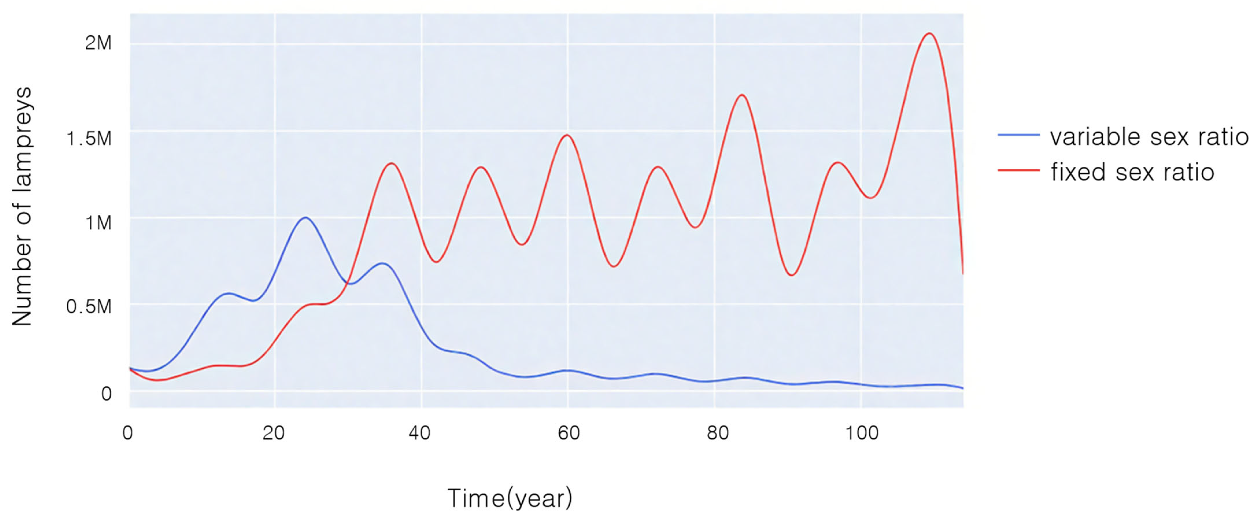
Figure 7 illustrates the variations in population sizes of two species over time under experimental conditions with the same initial sex ratio and initial age composition when sea lampreys with sex ratios that can change in response to the environment compete with sea lampreys with unchanging sex ratios.

From Figure 7, it can be seen that in the first 30 years, the population size of both lampreys tended to become larger, and the population size of sea lampreys with a variable sex ratio was significantly larger than that of those with a non-variable sex ratio. Thirty years later, the population size of sea lampreys with a non-variable sex ratio exceeded that of those with a variable sex ratio, and gradually tended to be in dynamic equilibrium, whereas the population size of lampreys with a variable sex ratio gradually became smaller and smaller, approaching nearly extinct status.

Figure 8 compares the differences of the following indices between the two populations:

Stability of population sex ratio: We set the initial male ratio of both lampreys to 0.7 and found that the male ratio of lampreys with an unchanged sex ratio gradually returned to normal, i.e., 0.5, while the male ratio of lampreys with a changeable sex ratio in the external environment was maintained at 0.7, with a tendency to increase.

Stability of age composition structure: For the juvenile ratio of both lampreys, we set the initial juvenile ratio of both at 0.96 and found that the juvenile ratio of lampreys with no change in sex ratio stayed at 0.96.

Reproductive success: Our finding indicates that the reproductive success rate of lampreys with an unchanged sex ratio gradually decreased, and the decrease was large, while the reproductive success rate of lampreys with a changeable sex ratio was maintained at about 0.7.

Environmental resource utilization: Regarding the resource utilization of the two species, it was found that the resource utilization of lampreys, which did not change their sex ratio, showed a decreasing trend and remained low for the first 20 years. On the other hand, the resource utilization of lampreys that can change their sex ratio following the external environment showed a significant upward trend, dynamically increasing from 10% to 70%.

From this, we can further conclude that the advantages of a variable sex ratio in lamprey populations include increased adaptability to environmental changes, the optimization of resource use, and reproductive success by adjusting the sex ratio.

We summarize the advantages and disadvantages of variable sex ratios in lamprey populations, and overall, if a population with variable sex ratios is allowed to compete with non-variable populations, it is not advantageous.

The advantages include increased resilience to environmental change by adjusting sex ratios to optimize environmental resource utilization and reproductive success. Within environments abundant in material resources, an increased number of females might promote swift population increase and proliferation. Such a mechanism may help populations to remain stable when environmental conditions change.

The disadvantage of this sex mechanism is that in resource-constrained and competitive environments, the population structure (composed of age composition and sex ratio) is unstable, and excessive bias toward one sex may lead to a reduction in genetic diversity. Over time, this could impact the population’s survival and reproductive capabilities.

We speculate that fluctuations in sex ratios may have an impact on other species in the ecosystem, altering the existing balance of the food chain, which will be discussed in subsequent sections. The impacts on ecosystems are complex and multifaceted, and further research is needed to gain a deeper understanding of the long-term impacts of sex ratio fluctuations on ecological balance and other species.

4. Adaptive Sex Ratio Impact Model (ASRI Model)

In this section, we will first use the Lotka–Volterra equation to construct the predation and prey models of lampreys according to the different roles they play in different ecosystems. Subsequently, by conducting experimental simulations, we aim to examine how lampreys affect species both upstream and downstream within the communal food web.

4.1. Predation and Prey Model Based on the Lotka–Volterra Equation

The role played by lampreys in the ecosystem is complex, whereby larvae live at the bottom of freshwater streams and feed mainly on microorganisms and organic matter in filtered water, considered to be parasites that have a significant impact on the ecosystem. Adult lampreys may migrate to different waters, including freshwater and brackish environments, and adult lampreys turn into predators, feeding on small fish, invertebrates, and so on. Concurrently, lampreys serve as a food source in certain global areas, including Scandinavia, the Baltic Sea, and among indigenous communities in North America’s Pacific Northwest. Therefore, we examine the role of lampreys as predators and prey in the food chain in the community separately. Figure 9 illustrates the varied functions of lampreys within the ecosystem dynamics.

Modeling of lampreys as predators

In this model, we assume that lampreys predominantly prey on a particular fish (the prey). Using the Lotka–Volterra equation [15], we can express this as:

Population growth equation for the prey(fish):

$${\displaystyle \frac{d{N}_{prey}}{dt}}=\left(r_{prey}-{\alpha }_1{N}_{lamp}\right)·N_{prey}$$

(26)

where $N_{prey}$ is the number of prey, $r_{prey}$ is its natural growth rate, $N_{lamp}$ is the number of predators (lampreys), and ${\alpha }_1$ is the predation rate coefficient. $r_{prey}{N}_{prey}dt$ is the naturally increasing number, and ${\alpha }_1{N}_{lamp}{N}_{prey}dt$ is the number of prey that are preyed upon. The quantity of prey being preyed upon is proportional to the number of prey and the predator, because only when predators and prey meet will predation occur.

Population growth equation for predator (lampreys):

$${\displaystyle \frac{d{N}_{lamp}}{dt}}=\left({\mathsf{\beta }}_1{\mathsf{\alpha }}_1{N}_{prey}-m_{lamp}\right)·N_{lamp}$$

(27)

where ${\mathsf{\beta }}_1$ is the transformation efficiency coefficient (the efficiency with which a preyis transformed into a new individual of the predator) and $m_{lamp}$ is the natural mortality rate of the predator (lampreys). ${\mathsf{\beta }}_1{\mathsf{\alpha }}_1{N}_{prey}{N}_{lamp}dt$ is the increase in the number of predators (lampreys) due to the hunting process. The additional coefficient in Equation (27) is because the predators may need to eat several times before they can produce new individuals, thus there is a transformation efficiency coefficient ${\mathsf{\beta }}_1$. $m_{lamp}{N}_{lamp}dt$ refers to the number of dead lampreys.

Modeling of lampreys as prey

In another scenario, we can consider lampreys as the prey and some larger predatory fish or other aquatic animal as the predator. The model equations can be set up similarly to obtain the following system of equations:

$$\left\{\begin{array}{c}{\displaystyle \frac{d{N}_{lamp}}{dt}}=\left(r_{lamp}-{\mathsf{\alpha }}_2{N}_{predator}\right)·N_{lamp}\\ {\displaystyle \frac{d{N}_{predator}}{dt}}=\left({\mathsf{\beta }}_2{\mathsf{\alpha }}_2{N}_{lamp}-m_{predator}\right)·N_{predator}\end{array}\right.$$

(28)

where $r_{lamp}$ is the natural growth rate of lampreys, ${\mathsf{\alpha }}_2$ is the predation rate coefficient, and $N_{predator}$ is the number of predators. ${\mathsf{\beta }}_2$ is the transformation efficiency coefficient, and $m_{predator}$ is the natural mortality rate of predators.

4.2. Results and Analysis of Modeling the Role of Sex Change in the Food Chain

We use the predator–prey model established previously, and the experimental results are shown and analyzed.

The first is an experimental simulation of a scenario in which lampreys serve as prey, and the results obtained are shown in Figure 10.

The left picture of Figure 10 shows the trend of the male proportion of lampreys over time after predation, which corresponds to the trend of the seven-gill lampreys and predator populations over time shown in the right picture of Figure 10. It can be seen that, as the number of lampreys increases, the male proportion of the lampreys shows a gradual decline and the number of predators rises with a time lag; then, the increase in the number of predators results in a large number of lampreys being preyed upon. There was a significant drop in lamprey populations and a rise in male lamprey numbers, and over time, predator numbers also fell swiftly due to reduced food availability.

Subsequently, there was a simulated experiment where lampreys functioned as predators, with the outcomes depicted in Figure 11.

The left panel of Figure 11 shows the trend in the proportion of male sea lampreys as predators over time, which matches the trend in the number of sea lampreys over time shown in the right panel of Figure 11. Moreover, it can be observed that as the number of prey increases, the proportion of males in sea lampreys gradually decreases, while the number of sea lampreys themselves rises. There is the same time lag, and then the increase in the number of sea lampreys leads to a large number of prey being preyed upon and a sharp decrease in numbers, while the proportion of male sea lampreys rises. After a period of time, the number of prey also gradually increased due to the decrease in the number of sea lampreys.

In summary, we have experimentally obtained conclusions about the effects of variable sex in lamprey populations on the ecosystem. Changes in lamprey sex ratios have important effects on the food web, and changes in the sex ratio of lamprey populations indirectly affect species upstream and downstream of their food chain by altering reproduction rates and population sizes. For example, population growth due to an increase in the proportion of females may increase predation pressure on downstream prey species while providing more food resources for upstream predators when food conditions become more abundant.

In addition, population dynamics due to changes in sex ratios may affect other species, such as parasites and species in symbiotic relationships. These important effects will be discussed in the subsequent sections, and in the next section, we will examine their implications for ecosystem stability.

5. Sex Ratio Impact on Ecosystem Stability Model (SRIES Model)

In this section, we will first develop a simple logistic model of population growth. Subsequently, we refine the basic model by considering the life cycle stage traits and the sex differentiation variability among the sea lamprey population. Evaluate how this unique seven-gill trait impacts individual organism populations in the ecosystem where it has a distinct relationship, such as symbiotic or parasitic, and conduct both practical and experimental evaluations of the model’s application and testing.

5.1. A Simple Logistic Model of Population Growth

In this case, we adopt Assumption 4. Additionally, the following four assumptions are made about the lamprey population in a given region:

• Assumption 2: The effect of migration of lamprey individuals in and out of the population on population size is not considered.
• Assumption 4: The carrying capacity of the environment in a given region is constant and does not change over time.
• Assumption 5: The population is homogeneous and all individuals within the population are physiologically and behaviorally identical.
• The population growth rate is constant, without considering the effects of changes in sex ratio and age composition.

We define the average number of lamprey species as $N$. According to the Logistic model, this number increases over time without exceeding the environmental carrying capacity $K$. We have

$${\displaystyle \frac{dN}{dt}}=rN\left(1-{\displaystyle \frac{N}{K}}\right)$$

(29)

where $r$ is the intrinsic growth rate, $K$ is the maximum average number of the species within the environmental limit, and ${\displaystyle \frac{dN}{dt}}$ is the rate of change in population size over time.

However, practical application to lampreys as a population requires the consideration of hypothetical limitations, particularly in variable natural and artificial environments. Lampreys have a uniquely distinct three-stage life cycle, and sex ratios are influenced by food availability, so environmental carrying capacity is not constant in growing environments with variable food availability, which in turn leads to non-constant population growth rates by affecting age composition and sex ratios. At the same time, the contribution of lampreys of different sexes to the population is different because males or females show different sex dominance in environments with different food conditions [1,11].

5.2. Symbiotic Sex Ratio Dynamics Model (SSRDM)

The objective of this model is to analyze how changes in sex ratios within lamprey populations affect the dynamics of related populations in an ecosystem under symbiotic relationships. The model takes into account the interactions between the two populations and introduces a logistic growth function to simulate the self-limiting properties of population growth [16,17].

Growth modeling of population 1:

$${\displaystyle \frac{d{x}_1}{dt}}=r_1{x}_1\left(1-{\displaystyle \frac{x_1}{N_1}}+a_1{\displaystyle \frac{x_2}{N_2}}\right)$$

(30)

where $x_1$ and $x_2$ are the numbers of the two populations, $r_1$ is the natural growth rate of population $1$, $N_1$ and $N_2$ are the environmental carrying capacities of population $1$ and population $2$, respectively, and $a_1$ is the coefficient of influence of population $2$ on the growth of population $1$.

Growth model for population 2:

$${\displaystyle \frac{d{x}_2}{dt}}=r_2{x}_2\left(1-a_2{\displaystyle \frac{x_1}{N_1}}-{\displaystyle \frac{x_2}{N_2}}\right)$$

(31)

where $r_2$ is the natural growth rate of population $2$ and $a_2$ is the coefficient of influence of population $1$ on the growth of population $2$.

5.3. Host–Parasite Sex Ratio Dynamics Model (HPSRDM)

The purpose of this model is to help us understand how changes in sex ratios within host populations can affect the growth and spread of host populations, and how this interaction can, in turn, affect the health and number of host populations [18].

Modeling the growth of host populations:

$${\displaystyle \frac{dH}{dt}}=r_{H}H\left(1-{\displaystyle \frac{H}{K_H}}\right)-\alpha PH$$

(32)

where $H$ is the number of host populations, $r_H$ is the natural growth rate of the host, $K_H$ is the environmental carrying capacity of the host, $\alpha$ is the parasitism rate coefficient, and $P$ is the number of parasitized populations.

Growth modeling of parasitized populations:

$${\displaystyle \frac{dP}{dt}}=\beta PH-\mu P$$

(33)

where $\beta$ is the transformation efficiency of the parasitized population to acquire new parasites from the host population and $\mu$ is the mortality rate of the parasitized population.

5.4. Application and Analysis of Extended Models

We conducted experimental simulations of symbiotic and parasitic relationships associated with lampreys, respectively, and the results obtained are shown below.

As shown in Figure 12, we also explored salmonids that have a symbiotic relationship with lampreys to plot the number of interactions between them over time. It can be found that their population number changes are basically synchronized, which is consistent with the basic model of a mutually beneficial symbiotic relationship. However, a noticeable delay persists, given that their populations are simultaneously constrained by environmental capabilities.

As shown in Figure 13, our model further explores four parasites that have parasitic relationships with lampreys, plotting their number over time at 20-year intervals. It can be seen that a gradual increase in the sex ratio of lamprey populations is accompanied by an increase in the number of Nematodes and Trematodes, in contrast to the changes in Arthropods and Protozoans. Thus, the proportion of males in lampreys is positively correlated with Nematodes and Trematodes.

In summary, sea lamprey populations provide an advantage to other species in the ecosystem, while there are only general symbiotic interspecific interactions with species in symbiotic relationships. Changes in sex ratios may affect the host selection and transmission strategies of parasites, as lampreys of different sexes may be different physiologically and behaviorally. This may affect parasite life cycles and spread rates, alter the dynamics of host–parasite relationships, and affect species diversity and stability in ecosystems. Models can be used to predict and develop strategies to control the spread of parasitized populations, especially when considering how to reduce parasitism pressure by managing host population sex ratios.

6. Variable Sex Ratio Ecosystem Interaction Model (VSREI Model)

This part delves into the impact of the sea lampreys on the entire ecosystem, modeling its stability via hierarchical analysis and examining the influence of sex ratio alterations on ecosystem stability.

6.1. Definition of Quantitative Indicators

Before conducting the hierarchical analysis, we first define several quantifiable indicators associated with ecosystem stability. The ecological definition of ecosystem stability is mostly a combination of resistance stability and resilience stability, which is defined in the context of disturbance. Furthermore, our aim is to employ measures not related to disruptions but closely linked with stability, in conjunction with the initial two metrics, to thoroughly evaluate stability and consider the degree of community number fluctuation and the community structure robustness index. The definitions of each are given in Figure 14.

Resistance and Resilience

Cluster parameters have a mean and time variance of $y_0$, shown here by $95\%$ confidence intervals around the mean. Impulse perturbations end at time $t_0$ (or stress perturbations begin) and parameters change $\left|y_0-y_L\right|$ after a time lag $\left|t_L-t_0\right|$ [19].

The resistance ($RS$) is an index of the magnitude of this change.

$$RS=1-{\displaystyle \frac{2\left|y_0-y_L\right|}{y_0+\left|y_0-y_L\right|}}$$

(34)

The resilience ($RL$) is an exponent of the rate of return to $y_0$ after the lag period,

$$RL=\left({\displaystyle \frac{2\left|y_0-y_L\right|}{\left|y_0-y_L\right|+\left|y_0-y_n\right|}}-1\right)÷\left(t_n-t_L\right)$$

(35)

where $y_n$ is the value of the parameter at the measurement time $t_n$, which indicates the recovery after a certain period of time.

Degree of community number fluctuation and community structure robustness index

Assuming that there are $k$ species in the community, the degree of fluctuation of the $k$ species is weighted and summed, and the degree of fluctuation is measured by the population number variance. Then, the expression for the degree of fluctuation of the community is

$$\sum _{k}Var\left(N_k\right)=\sum _k\underset{T}{\int }{\left(N_k-\overline{N_k}\right)}^{2}dt÷\underset{T}{\int }dt$$

(36)

where $\overline{N_k}$ is the average number of species $k$, expressed as

$$\overline{N_k}={\displaystyle \frac{{\int }_T{N}_{k}dt}{T}}$$

(37)

The community structure robustness index refers to the weighted sum of the number of individual populations in the community, where the weighting coefficient is related to the contribution of the species in maintaining the stability of the community. The expression is

$$Q=\sum _k{g}_k·N_k$$

(38)

where $g_k$ is the community structure coefficient.

6.2. AHP-Based Ecosystem Stability Model

The Analytic Hierarchy Process (AHP) allows us to assess the impact of sex ratio changes on ecosystem stability by integrating four quantitative indicators into a comprehensive evaluation model. This approach allows us to identify the influences that are important for ecosystem stability by comparing and weighing different indicators.

Analyzing the impacts in pairs resulted in a judgment matrix derived from significance assessments.

$$\left[\begin{array}{cccc}1& 3& 1/6& 1/4\\ 1/3& 1& 1/7& 1/5\\ 6& 7& 1& 3\\ 4& 5& 1/3& 1\end{array}\right]$$

In the aforementioned matrix, the initial row, second row, third row, and fourth row symbolize resistance, resilience, fluctuations in community number, and the robustness index of the community structure, respectively. Columns one, two, three, and four in the preceding matrix also symbolize resistance, resilience, fluctuations in community number, and the robustness index of community structure. The figures in the matrix symbolize the varied interrelations of significance across the parameters. We allocated values to the pairwise comparison matrix following our judicious assessment:

(1)

Given RS’s significance in short-term stability, it was deemed somewhat more crucial than RL, leading us to allocate a value of 3.

(2)

RS was considered less critical compared to the robustness index, given that the system’s long-term stability hinges more on its structural strength, leading us to allocate a value of 1/6.

(3)

RL was deemed marginally less significant compared to the robustness index, leading to a rating of 1/5.

We then need to check the consistency of the judgment matrix and evaluate it with a consistency ratio (CR). $CR$ can be calculated by Equation (39).

$$CR={\displaystyle \frac{CI}{RI}}$$

(39)

where $CI$ is the consistency index and $RI$ is the stochastic index.

$CI$ is calculated by Equation (40).

$$CI={\displaystyle \frac{{\mathsf{\lambda }}_{max}-n}{n-1}}$$

(40)

where ${\lambda }_{max}$ is the maximum eigenvalue of the judgment matrix. The correspondence between n and RI can be obtained by looking up the table.

We then calculated ${\lambda }_{max}=4.1725$, $CI=0.0575$, $CR=0.0639<0.1$. The check was passed, indicating that the judgment matrix we set earlier is reasonable and effective. The weights of each factor are shown in Figure 15.

6.3. Analysis of the Impact of Sex Changes on Ecosystem Stability

We then conducted experimental simulations of lamprey populations with different sex ratios, applying the ecosystem stability model based on multilevel analysis developed in this chapter. The results from the experiments are displayed in

Table 2. The results of the AHP-based ecosystem stability model.

Male Ratio	Stability	Resistance	Number	Variance	Total Score	Rank
0.30	0.74	1.00	0.10	0.36	0.23	5
0.40	0.47	0.10	0.59	0.08	0.40	4
0.50	0.47	0.57	0.60	0.59	0.58	2
0.60	0.10	1.00	1.00	0.10	0.62	1
0.70	1.00	0.57	0.26	1.00	0.56	3

.

Based on the final rankings, we found that the sea lamprey population had the most favorable impact on ecosystem stability when the male ratio was about 0.60. When the male ratio was about 0.30, the sea lamprey population had the worst impact on ecosystem stability.

In summary, changes in the sex ratio will affect the degree of community number fluctuation and community structural robustness index by influencing reproductive strategies and population number distribution in the ecosystem, which further impacts community resistance and resilience. Changes in the sex ratio of lamprey populations will directly affect the fluctuation of their population size, and may also affect the predation and prey relationship of lampreys, thereby affecting the balance of the whole food web. The stability of an ecosystem depends on the complex interactions between the species within it, and changes in the internal structure of any one population may cause a chain reaction that affects the health and functioning of the entire system. Briefly, adaptive changes in sex ratios may increase the resistance of ecosystems to environmental change, while at the same time affecting their resilience and internal stability, especially in the face of large-scale or long-term environmental perturbations.

7. Sensitivity Analysis

This paper is mainly based on the Runge–Kutta algorithm to solve the model of the system of differential equations corresponding to the population change in lampreys, and some of the parameters are approximations of the ideal state. Nonetheless, the situation tends to be more intricate, particularly in the case of lampreys, a distinct species whose gender is influenced by their growth rate. Therefore, the practicality, scientific validity, and stability of this model should be further considered.

Specifically, considering that the hatching success of lampreys is closely related to the environmental temperature as well as the amount of food, this test perturbed the temperature and the amount of food within a certain range. To evaluate the model’s sensitivity, a comparison was made of the population trends of lampreys at various levels of disturbance over time.

Figure 16 shows the changes in the survival environment temperature of the lamprey population under different levels of disturbance. It can be found that in the short term, to a certain extent, the higher the temperature, the larger the population size and the more rapid the growth, while the lower the temperature, the smaller the population size and the slower the growth. The main reason is that the survival rate during the incubation period is closely related to the temperature, but in the long term, the difference in the size of different populations at the time of stabilization is relatively small. This also further validates the reasonableness of the present model, that when the external environment is suitable, the population size of lampreys is mainly limited by the environmental capacity.

Figure 17 shows the variation of the lamprey population under different levels of disturbance of the living environment food. It can be found that the richer the amount of food, the larger the size of its population. However, following approximately 35 years of growth, the disparity among various populations becomes less pronounced.

8. Conclusions and Discussion

Overall, we created a complex model, which contains the dynamics of the sex ratio and examines the effects of changes in the sex ratio on population and ecosystem stability. Through competitive modeling, we conclude that in resource-rich environments, changes in sex ratios can lead to rapid population expansion. However, in resource-limited environments, changes in sex ratios may lead to long-term reductions in the reproductive capacity of populations. Simulations also suggest that changes in the sex ratio of sea lampreys can help co-occurring species suppress overgrowth and adapt to complex environmental changes. In addition, the ecosystem was most stable when the male ratio was close to 0.6, and these findings provide useful guidance for developing ecological management strategies.

Previous studies by Zhuhua Ji et al. [20] did not portray how the sex ratio varies over time; however, our study clearly gives a picture of how the sex ratio varies over time under food shortage and sufficiency. Our research illustrates and validates that in shorter time cycles, females under restricted growth conditions face higher mortality because they require more energy for the development of reproductive organs [21], and the food-restricted group exhibits a higher male-to-female ratio. Over extended periods, changes in the sex ratio itself may affect the population as a whole, with a sharp decrease in population size, which in turn affects the amount of food available to individual sea lampreys, increasing the number of females. Alternatively, the sharp decrease in its population may have led to a specific sex-determination mechanism in the lampreys, making it more inclined to produce females to ensure the reproduction of the race. In addition, the numerical solution of the system of differential equations using the fourth-order Runge–Kutta method ensured the accuracy and stability of the model calculations, which provided reliable results for the complex ecological dynamics model. It was found that hatchery sea lampreys and juvenile sea lampreys accounted for a large proportion of the overall population size, with the sum of both exceeding 80%. This is most likely a protective mechanism for the organisms, breeding large numbers of eggs and larvae to cope with crises, adapt to nature, and ensure that there is a sufficient number of adult individuals.

In the sex ratio model, we focus on the characteristic changes in the sex ratio of sea lampreys with the external environment and simulate the external environmental parameters by introducing large fluctuations. Such an approach enhances the model’s adaptability, more accurately mirrors the unpredictability and extremity of the environment within the real ecosystem, and bolsters the model’s accuracy. The decrease in males and increase in females resulted in increased survival pressure on downstream prey while providing sufficient food for their upstream predators. This suggests that sea lampreys and their upstream and downstream populations produce mutual constraints on the number of organisms through this predatory relationship. In contrast, changes in the sex ratio did not have a specific effect on the symbiotic organisms and only affected the behavior of a portion of the parasitic organisms. The findings of our research indicate that optimal ecosystem stability occurs with a male sex ratio of 0.6. In the future, we will likely be able to adjust the number of species and ensure ecological balance through this specific constraint relationship.

Our study still faces certain limitations, as we overlooked how the living conditions of sea lampreys influence their gender ratio, in contrast to various studies [1,22], indicating a strong correlation between sex determinants and their living environment. Furthermore, during the establishment of the two population competition models, the focus was solely on the variance in total food quantity, omitting the intricate alterations in the average physical quantity of fish. Changes in this index will be influenced by a wider range of factors and require more complex modeling.

The growth rate of sea lampreys determines their sex after maturity, and their growth rate is, in turn, influenced by the adequacy of their food supply, a conclusion that is amply supported by our study. The number of invasive lampreys is an important factor in the collapse of local fishery resources [23,24], and it is very important to realize the control of sea lamprey populations and study the mechanism of sea lamprey sex determination for the conservation of fishery resources.

References

1. Johnson, N.S.; Swink, W.D.; Brenden, T.O. Field study suggests that sex determination in sea lamprey is directly influenced by larval growth rate. Proc. R. Soc. B Biol. Sci. 2017, 284, 20170262. [Google Scholar]
2. Elmhagen, B.; Ludwig, G.; Rushton, S.; Helle, P.; Lindén, H. Top predators, mesopredators and their prey: Interference ecosystems along bioclimatic productivity gradients. J. Anim. Ecol. 2010, 79, 785–794. [Google Scholar] [PubMed]
3. Smith, A.; Fulton, E.; Hobday, A.; Smith, D.; Shoulder, P. Scientific tools to support the practical implementation of ecosystem-based fisheries management. ICES J. Mar. Sci. 2007, 64, 633–639. [Google Scholar]
4. Wikle, C.K. Hierarchical Bayesian models for predicting the spread of ecological processes. Ecology 2003, 84, 1382–1394. [Google Scholar]
5. Wang, F.; Luo, Y.; Zhang, W.; Yu, Y. A Decomposition-Based Stochastic Multilevel Binary Optimization Model for Agricultural Land Allocation Under Uncertainty. Mathematics 2025, 13, 1213. [Google Scholar] [CrossRef]
6. Biau, G. Analysis of a random forests model. J. Mach. Learn. Res. 2012, 13, 1063–1095. [Google Scholar]
7. Fulton, E.A. Approaches to end-to-end ecosystem models. J. Mar. Syst. 2010, 81, 171–183. [Google Scholar]
8. Lurgi, M.; Ritchie, E.G.; Fordham, D.A. Eradicating abundant invasive prey could cause unexpected and varied biodiversity outcomes: The importance of multispecies interactions. J. Appl. Ecol. 2018, 55, 2396–2407. [Google Scholar]
9. Fort, H. On predicting species yields in multispecies communities: Quantifying the accuracy of the linear Lotka-Volterra generalized model. Ecol. Model. 2018, 387, 154–162. [Google Scholar]
10. Zhen, J.; Duan, J.; Zhao, Q.; Saheya, B. Effects of Gender Ratio Change on Lampreys Ecosystem. Math. Model. Its Appl. 2024, 13, 80–85. [Google Scholar]
11. Chang, M.-m.; Wu, F.; Miao, D.; Zhang, J. Discovery of fossil lamprey larva from the Lower Cretaceous reveals its three-phased life cycle. Proc. Natl. Acad. Sci. USA 2014, 111, 15486–15490. [Google Scholar] [PubMed]
12. Hardisty, M.W.; Potter, I.C. The Biology of Lampreys; Academic Press: London, UK, 1971. [Google Scholar]
13. Hardisty, M.W. Biology of the Cyclostomes; Springer: London, UK, 1982. [Google Scholar]
14. Li, C.; Sun, J.; Zhang, H. Introduction of Several Biological Population Models. Hans J. Comput. Biol. 2019, 9, 5. [Google Scholar]
15. Das, S.; Gupta, P. A mathematical model on fractional Lotka–Volterra equations. J. Theor. Biol. 2011, 277, 1–6. [Google Scholar] [PubMed]
16. Zhang, H.; Wu, Y. The Symbiosis Evolution and Equilibrium in City Community Based on Logistic Model. Ecol. Econ. 2016, 32, 73–76+114. [Google Scholar]
17. Gao, H.; Li, X. Hopf Bifurcation of Predator Prey Symbiotic Model with Time Delay. J. Jilin Univ. (Sci. Ed.) 2023, 61, 1339–1350. [Google Scholar]
18. Liu, H.; Li, Z.; Liu, Z.; Li, W. Complex non-unique dynamics in host-parasitoid model. J. Lanzhou Univ. (Nat. Sci.) 2009, 45, 53–59. [Google Scholar]
19. Shade, A.; Peter, H.; Allison, S.D.; Baho, D.L.; Berga, M.; Bürgmann, H.; Huber, D.H.; Langenheder, S.; Lennon, J.T.; Martiny, J.B. Fundamentals of microbial community resistance and resilience. Front. Microbiol. 2012, 3, 417. [Google Scholar]
20. Ji, Z.; Chen, J.; Wang, Z. A Study on Lampreys Population Based on Sex-Ratio-Related Growth-Balance Model. arXiv 2024, arXiv:2407.10411. [Google Scholar]
21. Beamish, F. Biology of the North American anadromous sea lamprey, Petromyzon marinus. Can. J. Fish. Aquat. Sci. 1980, 37, 1924–1943. [Google Scholar]
22. Pyrzanowski, K.; Zięba, G.; Marszał, L.; Leśniak, M.; Banasiak, D.; Przybylski, M. Do Endangered Lampreys Benefit from Water Pollution? Effect of Municipal Sewage Treatment Plant Operation on Growth and Abundance of the Ukrainian Brook Lamprey and the European Brook Lamprey. Water 2025, 17, 494. [Google Scholar] [CrossRef]
23. Ferreira-Martins, D.; Champer, J.; McCauley, D.W.; Zhang, Z.; Docker, M.F. Genetic control of invasive sea lamprey in the Great Lakes. J. Great Lakes Res. 2021, 47, S764–S775. [Google Scholar]
24. Goldsworthy, C.A.; Carl, D.D.; Sitar, S.P.; Seider, M.J.; Vinson, M.R.; Harding, I.; Pratt, T.C.; Piszczek, P.P.; Berglund, E.K.; Michaels, S.B. Lake Superior fish community and fisheries, 2001–2022: An era of stability. J. Great Lakes Res. 2025, 51, 102414. [Google Scholar]
Figure 1. Global distribution chart of lampreys. The numbers in the figure represent the number of adult lampreys, with the unit being hundreds. Red signifies a broad distribution of lampreys, yellow indicates a moderate dispersion, and green denotes a limited distribution.
Applsci 15 07680 g001
Figure 2. Models and problems.
Applsci 15 07680 g002
Figure 3. Growth diagram of the three stages of the lamprey life cycle [11].
Applsci 15 07680 g003
Figure 4. Relationship between the number changes in the three stages of lampreys.
Applsci 15 07680 g004
Figure 5. Growth and sex ratio of lampreys under different conditions of food availability.
Applsci 15 07680 g005
Figure 6. Age distribution of lamprey populations over time.
Applsci 15 07680 g006
Figure 7. Changes in population size over time during competition between two populations.
Applsci 15 07680 g007
Figure 8. Changes in the percentage of males, percentage of juveniles, reproductive success, and resource utilization during competition.
Applsci 15 07680 g008
Figure 9. Number transfer relationships between lampreys as predator and prey.
Applsci 15 07680 g009
Figure 10. Interactions between lampreys and predators.
Applsci 15 07680 g010
Figure 11. Interactions between lampreys and their prey.
Applsci 15 07680 g011
Figure 12. Symbiosis of lampreys.
Applsci 15 07680 g012
Figure 13. Parasitism of lampreys.
Applsci 15 07680 g013
Figure 14. Examples of quantitative definitions of resistance and resilience from ecology.
Applsci 15 07680 g014
Figure 15. Weight of each factor in the AHP-based model.
Applsci 15 07680 g015
Figure 16. Sensitivity of the model under the condition of applying different disturbances α to the ambient temperature.
Applsci 15 07680 g016
Figure 17. Sensitivity of the model under the condition of applying different disturbances β to the survival environment food.
Applsci 15 07680 g017