Co-Optimization of Vibration Suppression and Data Efficiency in Robotic Manipulator Dynamic Modeling

Abstract

In response to the limitations of vibration suppression performance caused by the difficulty in accurately modeling nonlinear friction during robotic manipulator dynamics parameter identification, this paper proposes a hybrid identification method based on a Broad Learning System (BLS) optimized by Particle Swarm Optimization (PSO). First, a joint excitation trajectory is designed using a fifth-order Fourier series with zero boundary conditions to ensure sufficient excitation of system dynamics. Then, a linear regression formulation of the manipulator’s structural dynamics is established, and the BLS network is employed to model the unstructured residuals—primarily arising from nonlinear friction—with high precision. Finally, the PSO algorithm is applied to optimize the hyperparameters of the BLS network, achieving global model optimality. Simulation results demonstrate that under typical motion conditions of the manipulator, the proposed method exhibits excellent capability in capturing nonlinear disturbances, maintaining joint prediction errors below 6 × 10⁻¹² N·m. This significantly improves the accuracy and robustness of the feedforward vibration suppression control. Moreover, by integrating PSO-based hyperparameter optimization and trajectory design with sufficient excitation, the proposed method enhances data efficiency during the identification process, offering a novel and practical identification strategy for precise modeling and control of complex mechanical systems.

1. Introduction

With the widespread application of industrial robots in high-precision machining, aerospace manufacturing, and medical automation, the requirements for control accuracy and dynamic performance of robotic manipulators have become increasingly demanding. However, structural vibration has emerged as a major bottleneck hindering further performance improvement. In practical operations, due to structural flexibility, varying payloads, drive backlash, and nonlinear factors such as friction, robotic manipulators are prone to residual vibration, flexible vibration, and self-excited vibration during high-speed movements and frequent start-stop operations. These vibrations result in decreased positioning accuracy, prolonged execution time, and compromised system stability [1].

Recent studies have focused extensively on identifying the sources of vibration. Bai et al. proposed a torque compensation method based on a tracking filter, demonstrating that constructing a feedforward term by estimating acceleration can effectively suppress the peak response of residual joint vibrations in robotic manipulators [1]. Li et al. further highlighted that abrupt variations in trajectory jerk (i.e., the derivative of acceleration) are also key contributors to vibration. By optimizing spline trajectory parameters using a Quasi-Genetic Algorithm (QGA), they significantly reduced jerk variance, thereby suppressing vibrations at the source [2]. To meet the dual demands of vibration suppression and high-precision control, Zou et al. introduced a composite control strategy combining Zero-Vibration (ZV) input shaping and a Pole-placement Predictive Function Controller (PPFC). By employing gravity-compensated quasi-linear joint dynamics, the system was decoupled into four parallel first-order subsystems. On a 3-DOF manipulator, this method achieved a 45% reduction in tracking error, a 78% suppression of residual vibration, and a 32% reduction in motor torque fluctuations [3], thereby validating the effectiveness of the feedforward-feedback composite architecture in flexible joint control. Pereira et al. proposed a feedforward control method based on Time-Varying Filtered B-splines (TVFBS), which successfully suppressed residual vibrations in a 6-DOF robotic manipulator while maintaining operation speed. Compared to conventional Time-Varying Input Shaping (TVIP) methods, this approach improved trajectory tracking accuracy and established a modeling framework for the frequency response function applicable to multi-joint robotic systems [4].

However, the aforementioned methods typically rely on accurate modeling of the system’s frequency response, which limits their applicability when dealing with unstructured disturbances such as frictional hysteresis and environmental perturbations. These approaches are often based on idealized models or are restricted to trajectory-level regulation, lacking precise nonlinear dynamic identification and modeling support for the system itself. Therefore, under complex nonlinear disturbances, constructing a high-precision dynamic model remains a major challenge for implementing active vibration control. Although traditional mechanism-based modeling methods can analytically estimate inertial parameters, they fall short in accurately characterizing unstructured disturbances such as harmonic drive flexibility and time-varying friction hysteresis. As a result, the deviation between the model-predicted torque and the measured torque often exceeds 18.5% [5]. This underscores the necessity for a novel identification method that operates without the assumption of frictionless modeling—one that can autonomously learn the dynamic behavior of friction and support online parameter optimization. Conventional identification methods are primarily based on Newton–Euler or Lagrangian dynamics and are widely used in rigid manipulator systems. In these frameworks, inertial and center-of-mass parameters are typically estimated using linear Least Squares (LS) or Recursive Least Squares (RLS) algorithms. Yousefi et al. proposed a friction compensation approach by embedding experimentally validated LuGre friction models into a state feedback controller for motor-mechanical systems. Moradi et al. further extended this approach by incorporating nonlinear least squares into a sliding-mode control structure to enable time-varying friction identification, thereby achieving high-precision trajectory tracking for multi-DOF robotic [6].

In robotic manipulator systems characterized by flexible joints, harmonic drives, and strong structural coupling, the system response contains a substantial amount of nonlinear and dynamic disturbance components. Traditional structural models struggle to capture the complex frictional effects and load coupling characteristics inherent in such systems. To address these challenges, increasing attention has been directed toward unstructured modeling approaches. Zhu and Mao employed a BackproPagation (BP) neural network architecture to learn the mapping between inputs and outputs autonomously, treating network weights as parameters to accomplish inertial parameter identification tasks [7]. Parvaresh et al. compared the performance of Auto-Regressive with eXogenous (ARX) and Nonlinear Auto-Regressive with eXogenous (NARX) models in continuum robotic systems, and they found that the NARX model provided a more accurate description of nonlinear dynamic characteristics [8]. Hashim et al. utilized a BackPropagation Multilayer Perceptron (BPMLP) to perform nonlinear dynamic modeling of a flexible beam structure with fixed-free boundary conditions. In comparison with the traditional RLS method, the neural network exhibited superior accuracy in both time and frequency domains. The effectiveness of the model was validated through correlation tests and prediction error analysis, offering a solid foundation for the subsequent design of vibration suppression controllers [9]. However, these methods often suffer from high training complexity, difficulty in online parameter updating, and limited generalization capability.

To establish a nonlinear dynamic model under vibration control, recent research has begun to incorporate intelligent optimization algorithms to assist in parameter identification. Pinitnanthakorn et al. proposed a method combining Haar wavelet transformation with PSO, which enhanced nonlinear modeling capability through signal compression and global optimization. This approach successfully controlled the identification error of a multi-DOF robotic manipulator within 2% [10]. Wu et al. applied the identified parameters in a Nonlinear Model Predictive Control (NMPC) framework, constructing feedforward compensation for friction, thereby improving trajectory tracking performance in six-axis robotic systems [11]. The BLS, first introduced by Chen et al. in 2017 [12], constructs a width-expandable network using a combination of feature mapping and enhancement nodes. By employing pseudoinverse or regularized least squares to solve output weights, BLS avoids the iterative gradient-based training process typically required in conventional neural networks [12]. Feng et al. applied BLS to nonlinear system modeling and control by developing a fuzzy incremental BLS architecture, enabling online learning and control of complex systems [13]. Liu et al. embedded BLS into the control of a micromanipulation platform to perform small-sample nonlinear identification, successfully modeling microscale friction disturbances and achieving robust control [14]. Due to its fast training speed and support for incremental parameter updates, BLS is particularly suitable for friction modeling in industrial robots where fast response and dynamic adjustment are essential.

In robotic manipulator systems, complex disturbances such as nonlinear friction, flexible joint connections, and inertial mismatches are key contributors to high-frequency micro-vibrations and low-frequency residual oscillations. To achieve precise vibration suppression control, it is essential to accurately model the nonlinear dynamic disturbance components within the system. However, since the BLS involves a large number of randomly initialized parameters-such as the number of feature nodes, weight initialization ranges, and the configuration of enhancement layers-these hyperparameters significantly affect the model’s convergence speed and prediction accuracy during practical implementation. Under constrained excitation trajectories, it becomes increasingly difficult to fully characterize nonlinear disturbances using only the structural regression matrix. Therefore, incorporating evolutionary algorithms to optimize the model has become an important means of enhancing identification performance. Similar “nonstructural disturbance + parameter optimization” frameworks have been shown to improve torque estimation accuracy, particularly in low-speed regimes [15].

In summary, although existing methods have made certain progress in parameter identification for vibration control, several limitations remain. These include a heavy reliance on physical modeling [6], high computational cost associated with neural network training [7], lack of controller-compatible interfaces in some optimization approaches, and inadequate handling of multimodal nonlinear behaviors [16].

To address these challenges, this paper proposes a dynamic identification method that integrates the BLS with PSO. The proposed approach takes joint state variables as inputs and employs the BLS to model nonlinear friction, thereby constructing a nonstructural mapping from joint states to frictional torque and overall torque responses. This framework enables automatic learning of the frictional dynamic response without relying on explicit model assumptions. Meanwhile, PSO is used to optimize the structural and hyperparameters of the BLS network, enhancing the global accuracy of the identification model. In addition, by combining trajectory excitation design with the efficient structure of BLS, the method reduces the dependency on large-scale training datasets, thereby improving data efficiency and adaptability in real-world robotic applications.

The remainder of this paper is organized as follows: Section 2 presents the dynamic modeling and excitation trajectory design of the flexible-joint manipulator. Section 3 introduces the BLS-PSO-based identification method and its implementation. Section 4 discusses simulation results and analyzes the effectiveness of the proposed method. Finally, conclusions and future work are given in Section 5.

2. Dynamic Modeling and Linearization

In the design of vibration-suppression-oriented control strategies for robotic manipulators, an accurate dynamic model serves as a critical foundation for parameter identification and model-based compensation. To establish a high-precision dynamic model suitable for parameter identification under vibratory conditions, the Newton–Euler method is employed to derive the rigid-body dynamic equations. Subsequently, the technique of minimal parameter set construction is applied to formulate a linear regression form suitable for identification. In addition, the influence of unstructured disturbances such as friction and joint flexibility is taken into account, leading to a matrix representation of the mass matrix. This formulation provides a theoretical basis for the integration of nonstructural compensation models in subsequent sections.

The modeling framework adopted in this paper builds upon classical rigid-body dynamics and joint flexibility representations commonly used in robotic systems [3]. While the fundamental equations follow established principles, the overall modeling process, including the combination of flexible joint dynamics, zero-boundary Fourier excitation trajectories, and subsequent data-driven disturbance modeling is independently designed and implemented by the authors to support the proposed identification method.

2.1. Dynamic Modeling

The Newton–Euler method is one of the most widely used approaches for robotic manipulator modeling in both industrial and academic settings. Compared to the Lagrangian formulation, it offers higher computational efficiency and a superior recursive structure, particularly when dealing with multi-degree-of-freedom (multi-DOF) systems. This method establishes a complete dynamic mapping between joint state variables and system outputs by performing bidirectional recursion at both the kinematic and dynamic levels [17]. In terms of controllability and practical implementation, the Newton–Euler method is more suitable for industrial servo control systems, as it allows for better integration with parameter identifiers and feedforward compensators [16]. Based on this approach, the system utilizes forward recursion to describe the time-varying dynamic relationships between joint drives and connected links. Let the angular velocity and linear velocity of the $i$-th link be denoted as ${\omega }_i$ and $v_i$, respectively, where $A_i$ denotes the transformation matrix of link i, and $q_i$ is the joint angle of joint i.

The corresponding recursive formulations are given in Equations (1) and (2):

$$v_i=A_{i-1}{v}_{i-1}+f_i\left(q_i,{\dot{q}}_i\right)$$

(1)

$${\omega }_i =A_{i-1}{\omega }_{i-1}+g_i\left({\dot{q}}_i,{\ddot{q}}_i\right)$$

(2)

Based on the rigid-body inertia law and the principle of momentum conservation, the dynamic equilibrium equation for a single joint can be formulated as shown in Equation (3):

$${\tau }_i=J_i^T\left(f_i^{\mathrm{e}\mathrm{x}\mathrm{t}}+m_i{a}_i\right)$$

(3)

Here, $J_i^T$ denotes the Jacobian matrix of the $i$-th link, $f_i^{\mathrm{e}\mathrm{x}\mathrm{t}}$ represents the external disturbance force, and $m_i$ is the mass of the corresponding link. The complete rigid-body dynamic equation of the manipulator system can then be summarized as shown in Equation (4):

$$\tau =M(q)\ddot{q}+C(q,\dot{q})\dot{q}+G(q)+{\tau }_{\mathrm{fric} }$$

(4)

In this context, $M(q)$ represents the joint-space inertia matrix, $C(q,\dot{q})$ denotes the centrifugal and Coriolis torque terms, $G(q)$ is the gravity vector, and ${\tau }_{\mathrm{fric} }$ corresponds to the disturbance torque induced by friction. To provide a clearer representation of the contribution of each dynamic component to the joint output torque, Equation (4) can be further refined into Equation (5), which is expressed as follows:

$${\tau }_i={\sum }_{j=1}^n{M}_{ij}(q){\ddot{q}}_j+C_i(q,\dot{q})+G_i(q)+{\tau }_{f,i}+{\tau }_{\mathrm{e}\mathrm{x}\mathrm{t},i}$$

(5)

$$\left\{\begin{array}{l}{\sigma }_w=0.1u_{20}\hfill \\ {\displaystyle \frac{{\sigma }_u}{{\sigma }_w}}={\displaystyle \frac{{\sigma }_v}{{\sigma }_u}}={\displaystyle \frac{1}{{(0.177+0.000823h)}^{0.4}}}\hfill \end{array}\right.$$

(6)

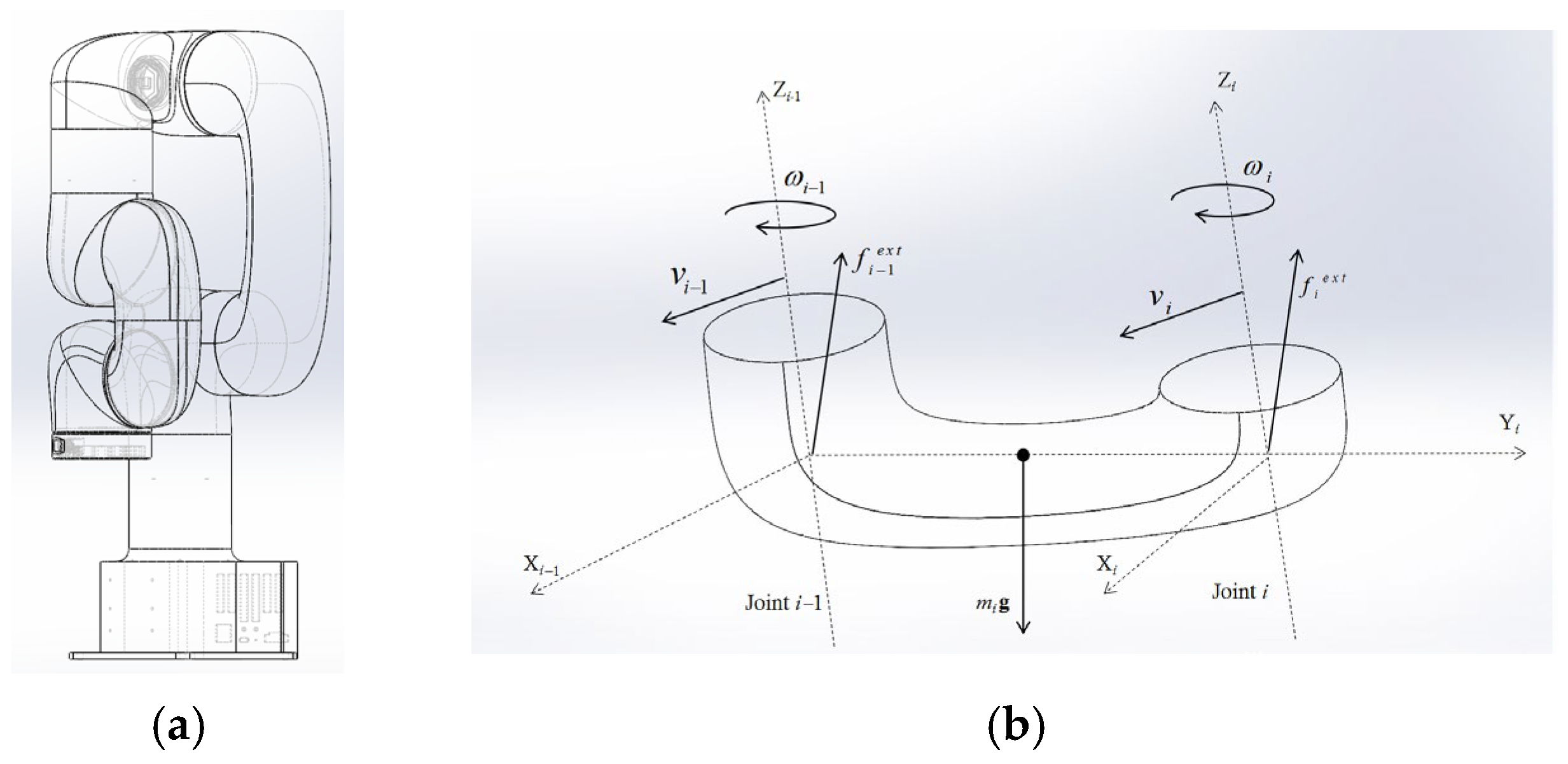
Here, ${\tau }_i$ represents the total output torque of the $i$-th joint, $M_{ij}(q)$ denotes the elements of the joint inertia matrix, and ${\tau }_{ext,i}$ represents the potential external disturbance terms. This expression provides the torque factors that form the basis for subsequent friction modeling and structural coupling analysis. The schematic of the dynamic parameters is shown in Figure 1. In Figure 1a, the SolidWorks model of a six-degree-of-freedom robotic manipulator is shown, indicating the mechanical structure adopted in this study. Figure 1b further defines the relevant kinematic and dynamic parameters on a single link, including angular velocity, linear velocity, gravity, link mass, and external disturbance forces, which are used in the modeling process.

2.2. Construction of Minimal Parameter Set and Linear Regression Expression

In robotic manipulator dynamic modeling, the original parameterized model often contains a large number of redundant parameters, such as masses, moments of inertia, and center-of-mass positions. This redundancy can lead to non-uniqueness of the solution or reduced identification accuracy. To improve the observability of the model and enhance the numerical stability of the identification system, the dynamic model is typically reconstructed into a Minimal Parameter Set (MPS) form and transformed into a standard linear regression structure, thereby enabling structure simplification for identification purposes.

In Equation (6), terms $M(q)$, $C(q,\dot{q})$, and $G(q)$ are all nonlinear functions with parameters embedded within the expressions, making direct identification difficult. To facilitate a structure suitable for least squares estimation, the model must be linearized and expressed in the form shown in Equation (7):

$$\tau =Y(x)\cdot P+\epsilon$$

(7)

Here, $x=\{q,\dot{q},\ddot{q}\}$ represents the state vector of the manipulator at the identification instant, $q$ denotes the joint position vector, $\dot{q}$ denotes the joint velocity vector, and $\ddot{q}$ denotes the joint acceleration vector. These state variables determine the instantaneous dynamic behavior of all physical quantities in the Newton–Euler formulation. Through algebraic transformation, the mass, inertia, and center-of-mass parameters are combined with structural constants into a minimal identifiable parameter set $P$. A linear regression matrix $Y(x)$ is constructed accordingly, and $\epsilon$ represents residual terms such as unmodeled disturbances or sensor noise.

From Equation (7), the linear regression form can be derived. To extract an explicit linear expression from the nonlinear dynamic model, an accurate regression matrix $Y$ is constructed, with its elements being functions of the state variables. These include joint angles, joint velocities, joint accelerations, and combination functions, which are related to the system’s inertia, Coriolis forces, and gravity terms. Based on the rigid-body dynamic characteristics of the robotic manipulator links, the minimal parameter set $P$ mainly includes:

$$P={\left[m_1,m_1{r}_{1x},m_1{r}_{1y},m_1{r}_{1z},I_{1,xx},I_{1,yy},I_{1,zz},f_{v1},f_{c1},\dots ,m_6,\dots ,f_{c6}\right]}^T$$

(8)

It mainly includes mass terms ${\mathrm{m}}_{\mathrm{i}}$, center-of-mass position terms $m_1{r}_{1y}$, moment of inertia terms $I_{1,xx}$, and friction parameter terms $f_{c1}$ [18]. To accommodate the structural identification requirements of a six-degree-of-freedom manipulator, the state variables $x=\{q,\dot{q},\ddot{q}\}$ are mapped into multiple dimensions of the regression matrix, as expressed in Equation (9):

$$Y={\left[\begin{array}{cccccc}{\ddot{q}}_1& {\dot{q}}_1& g& {\ddot{q}}_1{\dot{q}}_1& \mathrm{c}\mathrm{o}\mathrm{s}\left(q_1\right)& \dots \\ {\ddot{q}}_2& {\dot{q}}_2& g& {\ddot{q}}_2{\dot{q}}_2& \mathrm{c}\mathrm{o}\mathrm{s}\left(q_2\right)& \dots \\ ⋮& ⋮& ⋮& ⋮& ⋮& \ddots \\ {\ddot{q}}_6& {\dot{q}}_6& g& {\ddot{q}}_6{\dot{q}}_6& \mathrm{c}\mathrm{o}\mathrm{s}\left(q_6\right)& \dots \end{array}\right]}_{6\times m}$$

(9)

Since $Y$ contains certain columns that are linearly dependent, it is ill-conditioned and cannot be directly estimated using the least squares method. Therefore, QR decomposition is applied to transform it into a full-rank form [18], as shown in Equations (10) and (11):

$$Y_{min}=Y\cdot P_b$$

(10)

$$P_b=K\cdot P$$

(11)

Here, $K$ is the parameter transformation matrix, which extracts the unique inertial subspace. After transformation, $Y_{min}$ becomes the identification matrix with maximal observability.

2.3. Derivation of the Inertia Matrix

In flexible-joint robotic systems, each joint is modeled with two independent degrees of freedom to accurately capture the dynamics of both the actuator and the mechanical link. Specifically, we denote:

$\theta$ as the motor-side joint angle (i.e., actuator output) and $q$ as the link-side joint angle (i.e., physical displacement of the link).

The inertia matrix $M(q)$ represents the centralized expression of inertial coupling terms in the dynamic model, and its accurate modeling is crucial for predicting system responses and achieving high-precision torque estimation. Under vibration control conditions, the accuracy of the inertia matrix directly affects the performance of feedforward compensation and the system’s ability to isolate nonlinear disturbances. In systems with flexible connections or harmonic drive structures, the rigid-body inertia matrix fails to adequately capture the true dynamic characteristics of the system. Therefore, flexible coupling effects are introduced, with the expression given as:

$$J_{\mathrm{e}\mathrm{f}\mathrm{f}}\ddot{\theta }+K(\theta -q)+B(\dot{\theta }-\dot{q})=\tau$$

(12)

Here, $J_{\mathrm{e}\mathrm{f}\mathrm{f}}$ denotes the equivalent rotational inertia; $K$ and $B$ refer to the equivalent stiffness and viscous damping coefficient of the flexible connecting element. By introducing this structural formulation, the elastic hysteresis behavior of the flexibly coupled system can be effectively described.

Starting from the kinetic energy perspective, the inertia matrix structure of a six-degree-of-freedom manipulator is derived and reconstructed into a linear form suitable for identification. From the above, it is known that the link mass is denoted as ${\mathrm{m}}_{\mathrm{i}}$, the center-of-mass position as $r_i$, the angular velocity as ${\omega }_i$, and the rotational inertia tensor as $I_i$. The kinetic energy can be expressed as the sum of translational kinetic energy and rotational kinetic energy:

$$T={\sum }_{i=1}^6\left({\displaystyle \frac{1}{2}}{m}_i{\dot{r}}_i^T{\dot{r}}_i+{\displaystyle \frac{1}{2}}{\omega }_i^T{I}_i{\omega }_i\right)$$

(13)

Based on ${\dot{r}}_i=J_{v_i}(q)\dot{q}$ and ${\omega }_i=J_{{\omega }_i}(q)\dot{q}$, the total kinetic energy of the system can be obtained as:

$$T={\displaystyle \frac{1}{2}}{\dot{q}}^T\left({\sum }_{i=1}^6\left[m_i{J}_{v_i}^T{J}_{v_i}+J_{{\omega }_i}^T{I}_i{J}_{{\omega }_i}\right]\right)\dot{q}\triangleq {\displaystyle \frac{1}{2}}{\dot{q}}^{T}M(q)\dot{q}$$

(14)

From this, the explicit structure of the inertia matrix can be obtained, as shown in Equation (15):

$$M(q)={\sum }_{i=1}^6\left(m_i{J}_{v_i}^T{J}_{v_i}+J_{{\omega }_i}^T{I}_i{J}_{{\omega }_i}\right)$$

(15)

Using $M(q)$ as the fundamental modeling object, its importance in output torque estimation is validated [18]. Furthermore, to characterize the role of inertial coupling terms in a six-degree-of-freedom manipulator system, it is expanded into a matrix form:

$$M(q)=\left[\begin{array}{cccc}{M}_{11}& M_{12}& \dots & M_{16}\\ M_{12}& M_{22}& \dots & M_{26}\\ ⋮& ⋮& \ddots & ⋮\\ M_{16}& M_{26}& \dots & M_{66}\end{array}\right]$$

(16)

Each element in the matrix is a function of the joint angles, with the specific coefficients determined by the geometric and mass properties of each link. According to the Newton–Euler method, the inertial torque output of the system can be expressed as ${\tau }_{\mathrm{inertia} }$:

$${\tau }_{\mathrm{inertia} }=M(q)\ddot{q}={\sum }_{j=1}^6\left({\sum }_{i=1}^6{M}_{ij}(q){\ddot{q}}_j\right)e_i$$

(17)

This structure can be applied in the modeling stage of predictive control, explicitly defining the inertia matrix path and allowing for correction of the predictor structure based on the residuals of the regression matrix [19]. To construct the regression model, $M(q)$ and $\ddot{q}$ are reformulated as the product of the state regression matrix $Y_M$ and the minimal parameter vector $P_M$:

$${\tau }_{\mathrm{inertia} }=Y_M(q,\ddot{q})\cdot P_M$$

(18)

The main characteristic terms include polynomials such as $Y_M$, $cos\left(q_i\right){\ddot{q}}_i$, and $cos\left(q_i+q_j\right){\ddot{q}}_k$, while parameter $P_M$ contains variables related to mass inertia and inertial coupling, as shown in Equation (19),

$$P_M={\left[m_1,I_{1xx},m_1{x}_{c1},\dots ,I_{6zz},m_6{x}_{c6}\right]}^T$$

(19)

In identification experiments, the observability of 1 can be improved by designing specific trajectory excitation parameters, thereby ensuring that the regression matrix is of full column rank [20].

The inertia matrix is the dominant component in the excitation-response process, especially during rapid acceleration phases, where parameter distortion can directly cause abnormal outputs in the control system and trigger structural oscillations. Therefore, accurate reconstruction of $M(q)$ becomes a critical foundation for feedforward compensation and vibration source inference. This structure forms the core regression component of the linear identification process, serving as the basis for inertial parameter fitting. Moreover, its residuals are used as the input residuals for subsequent BLS training, providing the input source for friction disturbance modeling.

3. Nonlinear Identification Method Based on Broad Learning System and Particle Swarm Optimization

3.1. Construction of a Nonlinear Friction BLS Network

In the context of vibration control, unstructured disturbances such as frictional interference and structural coupling residuals are major contributors to system micro-vibrations and end-effector drift. To enhance the system’s ability to perceive such dynamic disturbances, a BLS with nonlinear fitting capability is introduced as the core of the vibration modeling module.

The BLS learns the mapping between input state vectors and friction torque, capturing friction dynamics directly and enabling feedforward compensation in subsequent vibration controllers.

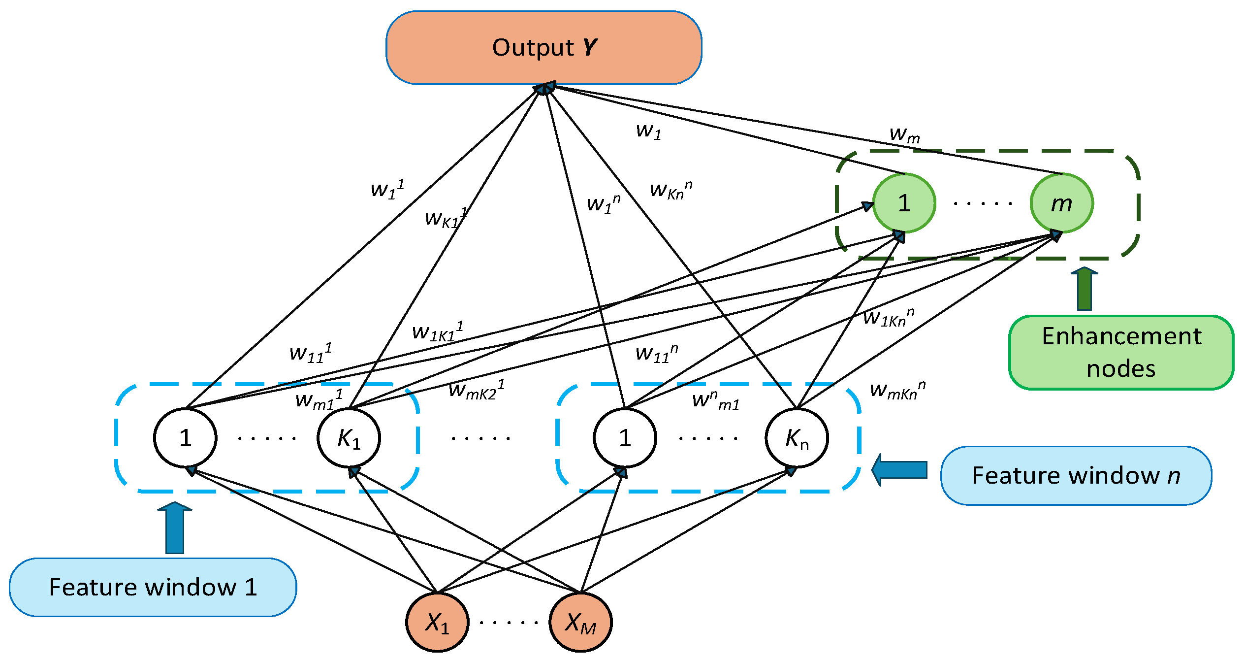
BLS is a shallow neural network and an efficient alternative to deep learning, utilizing a width-expansion strategy. It consists of a feature mapping layer, enhancement layer, and output layer, and replaces traditional deep architectures with lateral expansion. BLS exhibits strong adaptability in handling nonlinear systems. By applying multiple random mapping functions, the input data are projected into a high-dimensional feature space, and the target output is approximated using least squares estimation [12]. Figure 2 illustrates the structure of a BLS network.

The feature mapping layer of BLS transforms the input into a high-level feature space to approximate nonlinear functions. To better simulate velocity-dependent friction disturbances observed during robotic manipulator motion, the LuGre friction model is introduced as a physical reference form for unstructured disturbances. Its dynamic expression is given in Equation (20):

$$\dot{z}=\dot{q}-{\displaystyle \frac{\left|\dot{q}\right|}{{\sigma }_{0}g(\dot{q})}}z,{\tau }_f={\sigma }_{0}z+{\sigma }_1\dot{z}+{\sigma }_2\dot{q}$$

(20)

Here, $\mathrm{z}$ denotes the elastic displacement state of microscopic surface contact, ${\sigma }_0$ represents the stiffness coefficient of the model, ${\sigma }_1$ is the damping coefficient, and ${\sigma }_2$ is the viscous friction coefficient. Term $g(\dot{q})$ is defined as the velocity-based Stribeck function, used to simulate the nonlinear stick–slip decay behavior. The specific form of $g(\dot{q})$ is given in Equation (21):

$$g(\dot{q})={\tau }_c+\left({\tau }_s-{\tau }_c\right)e^{-{\left({\displaystyle \frac{\dot{q}}{v_s}}\right)}^2}$$

(21)

This structure characterizes the dynamic response of the friction torque to changes in joint velocity. Next, input $\mathrm{x}$ is constructed, and the joint state variables are defined as shown in Equation (22):

$$x=[q,\dot{q},\ddot{q}]\in R^3$$

(22)

Here, $q,\dot{q},\ddot{q}$ represents the joint angle, velocity, and acceleration, which are used as the input to the BLS network to effectively provide information about the friction disturbance variation under the current joint state. Subsequently, the feature mapping layer is constructed, where the input undergoes feature transformation. Each mapping channel applies a random weight and bias followed by an activation function, as expressed in Equation (23):

$$Z^{(i)}={\varphi }^{(i)}\left(x{W}_z^{(i)}+b_z^{(i)}\right)\in R^{1\times k},i=\mathrm{1,2},\dots ,m$$

(23)

Here, $W_z^{(i)}$ denotes the weights applied to the input for each mapping node; ${\varphi }^{(i)}$ is the activation function responsible for introducing nonlinear characteristics; and each $Z^{(i)}$ provides a set of corresponding high-dimensional features. All such features collectively form the total feature mapping matrix, as shown in Equation (24):

$$Z=\left[Z^{(1)},Z^{(2)},\dots ,Z^{(m)}\right]\in R^{1\times (m\cdot k)}$$

(24)

The feature-mapped inputs are passed to the enhancement layer, where complex nonlinear combinations are generated through enhancement functions:

$$H^{(j)}={\xi }^{(j)}\left(Z{W}_h^{(j)}+b_h^{(j)}\right)\in R^{1\times l},j=\mathrm{1,2},\dots ,n$$

(25)

By concatenating all enhancement nodes and generating the output, Equation (26) is obtained:

$$H=\left[H^{(1)},H^{(2)},\dots ,H^{(n)}\right]\in R^{1\times (n\cdot l)}$$

(26)

The final layer is trained through the output layer to fit the friction torque, resulting in the regression matrix:

$$A=[Z,H]\in R^{1\times M}$$

(27)

Let the target friction torque be denoted as ${\tau }_{\mathrm{fric} }^{\mathrm{target} }$; the training objective is to minimize the fitting error:

$${min}_W{‖A\cdot W-{\tau }_{\mathrm{fric} }^{\mathrm{target} }‖}_2^2$$

(28)

The weight $\mathrm{W}$ is the final output weight and can be directly used for friction torque prediction.

$${\hat{\tau }}_{\mathrm{BLS} }=[Z,H]\cdot W$$

(29)

To enhance the generalization ability and stability of the BLS network, a regularization loss function is introduced in the output layer training objective. Let $\mathrm{N}$ be the number of samples, ${\hat{\tau }}_i$ represent the predicted friction torque of the $i$-th sample by the BLS network, ${\tau }_i$ denote the corresponding ground truth, and $\lambda$ be the regularization coefficient used to suppress overfitting. The loss function is defined as shown in Equation (30):

$$\mathcal{L}(W)={\displaystyle \frac{1}{N}}{\sum }_{i=1}^N{\left({\tau }_i-{\hat{\tau }}_i\right)}^2+\lambda \Vert W{\Vert }_2^2$$

(30)

Compared to deep neural networks, the shallow and flexible architecture of BLS makes it particularly well suited for high-frequency vibration modeling, nonlinear friction learning, and non-uniform dynamic response modeling. In disturbed nonlinear systems, it offers improved identification accuracy and enhanced stability performance. Figure 3 shows the BLS simplified model under the non-linear system.

3.2. BLS Network Optimized by PSO

In the dynamic parameter identification of robotic manipulators under vibration suppression, the identification process is often affected by friction components and low-frequency structural vibrations. These factors may lead to output drift or distorted responses as excitation conditions change, particularly in the presence of nonlinear disturbances.

To address this issue, PSO is introduced to optimize the structural parameters of the BLS network, significantly enhancing its local fitting capability for nonlinear disturbances and improving the noise tolerance of the overall regression structure.

PSO is a swarm intelligence evolutionary algorithm proposed by Kennedy and Eberhart in 1995. It is inspired by the cooperative foraging behavior of bird flocks in multimodal environments. The algorithm dynamically adjusts the search path of each particle in a high-dimensional solution space through a dual-memory mechanism: individual best experience and global best performance. Compared with conventional optimization methods, PSO exhibits superior convergence stability and global search capability in high-dimensional nonlinear systems. It is especially effective in frequency response modeling and controller parameter tuning, where it offers strong overshoot suppression and response speed control [21].

The performance of the BLS model is influenced by multiple factors, including the number of feature mappings, the type of activation functions, and the regularization coefficient. Traditional heuristic methods struggle to find an optimal configuration in such a multidimensional parameter space, limiting the applicability of BLS in complex nonlinear disturbance scenarios. The introduction of PSO transforms the network training process into a parameter optimization problem: each particle represents a specific configuration of the BLS network and is evaluated through a fitness function (e.g., torque prediction error). The parameter update is guided by feedback from both individual and global optima. This approach not only improves the BLS network’s ability to locally fit nonlinear friction and flexible coupling disturbances but also enhances the robustness and generalization ability of the overall regression model.

Assuming a swarm of $N$ particles, the position update of each particle is determined by tracking its personal best and the global best positions, as defined in Equations (31) and (32):

$$v_i^{k+1}=w{v}_i^k+c_1{r}_1\left(p_i-x_i^k\right)+c_2{r}_2\left(g-x_i^k\right)$$

(31)

$$x_i^{k+1}=x_i^k+v_i^{k+1}$$

(32)

To further enhance the search effectiveness of the particle swarm and mitigate premature convergence, a constriction factor model $\mathsf{\chi }$ is introduced. This model controls the dynamic convergence rate of the step size and improves particle stability in complex parameter spaces. Its specific formulation is given in Equation (33):

$$\chi ={\displaystyle \frac{2}{\left|2-\phi -\sqrt{{\phi }^2-4\phi }\right|}}$$

(33)

The final expression is given in Equation (34):

$$v_i^{k+1}=\chi [w{v}_i^k+c_1{r}_1\left(p_i-x_i^k\right)+c_2{r}_2\left(g-x_i^k\right)]$$

(34)

Here, $\mathsf{\phi }$ represents the sum of $c_1$ and $c_2$; $x_i$ is the current position vector of the $i$-th particle; $v_i$ is the velocity vector; $p_i$ denotes the personal best position of the particle; $g$ is the global best position; and $w$ is the inertia weight.

To improve the boundary control capability during the particle swarm optimization process, the particles are initialized as shown in Equation (35):

$$x_i(0)\sim \mathcal{U}\left(x_{\mathrm{m}\mathrm{i}\mathrm{n}},x_{\mathrm{m}\mathrm{a}\mathrm{x}}\right),v_i(0)\sim \mathcal{U}\left(v_{\mathrm{m}\mathrm{i}\mathrm{n}},v_{\mathrm{m}\mathrm{a}\mathrm{x}}\right)$$

(35)

The initial positions and velocities of the particles are uniformly sampled within the upper and lower bounds to ensure global coverage of the search space and to prevent divergence due to boundary violations. The position boundaries are defined as shown in Equation (36):

$$x_i^{(t+1)}=\left\{\begin{array}{ll}{x}_{\mathrm{m}\mathrm{i}\mathrm{n}},& \mathrm{if} x_i^{(t+1)}<x_{\mathrm{m}\mathrm{i}\mathrm{n}}\\ x_{\mathrm{m}\mathrm{a}\mathrm{x}},& \mathrm{if} x_i^{(t+1)}>x_{\mathrm{m}\mathrm{a}\mathrm{x}}\\ x_i^{(t+1)},& \mathrm{otherwise} \end{array}\right.$$

(36)

A time-decay-based inertia weight annealing mechanism is introduced to enable global exploration in the early stage and smooth convergence in the later stage, as defined in Equation (37):

$$\omega (t)={\omega }_{\mathrm{m}\mathrm{a}\mathrm{x}}-{\displaystyle \frac{\left({\omega }_{\mathrm{m}\mathrm{a}\mathrm{x}}-{\omega }_{\mathrm{m}\mathrm{i}\mathrm{n}}\right)\cdot t}{T_{\mathrm{m}\mathrm{a}\mathrm{x}}}}$$

(37)

The final convergence criterion of the PSO algorithm is defined as:

$$\left|J_t-J_{t-1}\right|<ϵ$$

(38)

Equation (38) indicates that when the change in fitness between two consecutive iterations is less than threshold $ϵ$, the algorithm is considered to have reached a stable solution.

Through continuous iterative updates of the equations, each particle converges toward the optimal region in the global search space, thereby enhancing the nonstructural identification capability of the constructed BLS network. The objective of particle swarm optimization is to minimize the loss function defined based on identification error. Let $N$ be the number of training samples, $J$ the model output, and ${\hat{\tau }}_i$ the true torque values. The fitness function is then defined as shown in Equation (39):

$$J={\displaystyle \frac{1}{N}}{\sum }_{i=1}^N{‖{\hat{\tau }}_i-{\tau }_i‖}^2$$

(39)

This equation quantifies the mean squared error between the estimated torque output and the true torque under the current BLS network structure parameters. The optimization objective is to find the optimal combination of hyperparameters that minimizes this error.

3.3. Hybrid Optimization-Based Parameter Identification Framework

In dynamic parameter identification, traditional minimal parameter set regression models can provide a clear structural mapping from a physical modeling perspective. However, they often fail to ensure accuracy in output prediction and consistency in control response when faced with unstructured disturbances in real-world systems. Therefore, achieving high-precision torque estimation and effective subsequent vibration suppression control depends critically on the efficient integration of structural and nonstructural modeling approaches.

In the standard linear regression model based on the minimal parameter set, all dynamic characteristics of the system can be explained by structural terms. However, in practical systems, robotic manipulators are affected by unstructured disturbances that lack a unified modeling form. To enhance the model’s fitting capability and improve the accuracy of feedforward control compensation, nonstructural disturbance terms are introduced into the original structural model. The overall model can then be expressed as:

$$\tau (t)=Y\left(x_t\right)P+{\tau }_f(t)+e(t)$$

(40)

By combining the nonlinear modeling capability of the BLS with the global optimization ability of PSO, a unified framework is established for jointly modeling both the structural dynamic components and unstructured disturbances in robotic manipulators. In this mechanism, the minimal parameter set model serves as the foundation for capturing the primary structural dynamics, while the BLS is used to model residual terms arising from factors such as friction. PSO is employed to optimize the architecture and hyperparameters of the BLS network. Together, this forms a structure-driven hybrid identification framework that supports high-frequency vibration compensation and high-precision feedforward torque prediction. The structural model terms are estimated using the least squares method:

$${\hat{\tau }}_{\mathrm{struct} }(t)=Y\left(x_t\right)P$$

(41)

The residual is defined as:

$$r(t)=\tau (t)-\left({\hat{\tau }}_{\mathrm{struct} }(t)+K(\theta -q)+B(\dot{\theta }-\dot{q})\right)$$

(42)

This definition characterizes the residual as the main source of unstructured disturbances. To prevent it from propagating through the control system and exciting structural vibrations, it must be accurately modeled and suppressed. A disturbance modeling function is constructed using the BLS:

$${\hat{r}}_t={\mathcal{F}}_{\mathrm{B}\mathrm{L}\mathrm{S}}\left(x_t;W,\beta \right)$$

(43)

The final system identification model can be expressed as:

$$\hat{\tau }(t)={\hat{\tau }}_{\mathrm{struct}}(t)+{\hat{r}}_t=Y\left(x_t\right)P+{\mathcal{F}}_{\mathrm{B}\mathrm{L}\mathrm{S}}\left(x_t\right)$$

(44)

By integrating structural modeling with a disturbance compensation mechanism, the proposed model not only enhances the resolution of vibration source modeling but also significantly improves system prediction performance, reduces the amplitude of compensation excitation, and exhibits strong real-time update capability, making it suitable for feedforward control scenarios.

Figure 4 illustrates the control framework for compensating unstructured joint torque in robotic arms using a BLS-based friction modeling approach enhanced by PSO optimization. The system receives joint position, velocity, and acceleration as inputs, which are fed into both the nominal dynamic model and the friction modeling network. The dynamic model estimates the structured torque under ideal rigid-body assumptions, while the BLS friction network captures nonlinear residual components such as joint friction. These two outputs are combined to form the total estimated torque, which is then compared against the actual measured torque to calculate an error signal. This error serves as the fitness input for the PSO optimizer, which continuously adjusts the structure and parameters of the BLS network. The optimized results are passed through a weight updating module and fed back into the BLS network, enabling real-time adaptation. Through this closed-loop mechanism, the system incrementally improves its ability to model and compensate for unstructured torque components, thereby enhancing overall modeling accuracy and robustness.

3.4. Excitation Function Design and Sampling

Dynamic parameter identification relies on sufficient excitation of the system’s state space through input trajectories. In vibration-suppression-oriented parameter identification, the excitation trajectory must cover the full motion range of the joints while also activating subtle friction disturbances and flexible coupling modes, enabling the model to comprehensively identify unstructured sources that induce vibration. Insufficient excitation leads to incomplete coverage, resulting in degradation of the identification matrix and making it difficult to model errors, which may cause improper compensation in the control response [20].

To meet the requirements of identifiability, excitation smoothness, and periodic closure, a fifth-order Fourier excitation trajectory with zero boundary conditions is designed. Its basic form is given in the following equation:

$$q_{d,i}(t)={\sum }_{k=1}^5\left({\displaystyle \frac{a_{i,k}}{{\omega }_k}}sin\left({\omega }_{k}t\right)-{\displaystyle \frac{b_{i,k}}{{\omega }_k}}cos\left({\omega }_{k}t\right)\right)$$

(45)

Here, $q_{d,i}(t)$ represents the excitation displacement trajectory of the iii-th joint; ${\omega }_k$ denotes the base frequency of the $k$-th sine/cosine component; and $a_{i,k}$ and $b_{i,k}$ are the corresponding Fourier coefficients for the joint. All joint trajectories constructed using the zero-boundary Fourier series satisfy the constraint conditions defined in the following equation, which ensures smooth excitation and prevents non-physical vibration caused by discontinuities.

$$q_{d,i}(0)=q_{d,i}(T)=0,$$

(46)

$${\dot{q}}_{d,i}(0)={\dot{q}}_{d,i}(T)=0,$$

(47)

$${\ddot{q}}_{d,i}(0)={\ddot{q}}_{d,i}(T)=0.$$

(48)

To ensure that the sampled data can effectively excite the full state of the system, the excitation trajectory is sampled at 500 Hz, satisfying the Nyquist criterion. The trajectory period is set to 10 s to cover the complete cycles of all five Fourier orders, preventing truncation effects. The trajectory constraints ensure that both joint angles and velocities are zero at the start and end points, guaranteeing continuity and differentiability at the boundaries and avoiding false vibration responses caused by abrupt changes.

Figure 5 shows the zero-boundary fifth-order Fourier excitation trajectories for the robotic manipulator, representing the prescribed input signals at the motor-side. Here, J_i denotes the motor-side joint input angle for joint i, used to avoid ambiguity with other rotational variables. These trajectories are specifically designed as ideal reference signals to excite the robotic system sufficiently for dynamic parameter identification. It should be noted that these input trajectories do not depict the actual joint output responses, which would reflect additional vibrations due to joint flexibility and other nonlinear effects.

Table 1. Joint excitation trajectory parameters.

Joint Parameters	Joint 1	Joint 2	Joint 3	Joint 3	Joint 5	Joint 6
$q_{i,0}$	−0.1738	−0.0922	0.0631	−0.6137	0.4425	−0.0799
$a_{i,1}$	−0.7341	−0.0259	−0.1009	−0.8351	−0.7559	−0.6254
$b_{i,1}$	−0.6612	0.5541	−1.5451	−0.8694	0.7561	−0.5224
$a_{i,2}$	0.1784	0.0426	0.4528	0.2441	0.6617	0.7819
$b_{i,2}$	0.2216	2.6674	−0.3699	1.0831	0.9726	−0.7831
$a_{i,3}$	0.4174	1.5415	0.2490	0.3279	−0.5766	0.6088
$b_{i,3}$	0.2898	−0.5156	−0.2294	1.4351	0.6927	2.8099
$a_{i,4}$	0.4292	−0.7398	1.7237	−0.1248	−0.4196	−0.5076
$b_{i,4}$	0.8286	0.1477	1.2663	−0.0740	0.8642	−0.5941
$a_{i,5}$	−1.5795	0.6055	0.3583	0.7880	−0.8074	−0.3085
$b_{i,5}$	−0.9484	−0.3202	−1.6608	1.1983	1.9128	0.1656

lists the excitation trajectory parameters, which include the fifth-order Fourier coefficients used for all six joints. These coefficients correspond to the amplitude scaling factors for the sine and cosine components, defining the relative contribution of each frequency order within the excitation signal. They determine the spectral structure and time-domain energy distribution of the trajectory. These coefficients are directly used to generate the drive signals, which are applied in both simulation and physical experimental systems to collect modeling sample data, excite system dynamic responses, and ultimately support the modeling of unstructured disturbances and the identification of vibration characteristics.

4. Simulation Experiments

To validate the proposed system parameter identification method based on the integration of BLS and PSO, a series of simulations were conducted to assess its modeling performance under vibratory operating conditions. The proposed algorithm and associated simulation framework were implemented using MATLAB R2023b Specifically, the PSO optimization algorithm was programmed using MATLAB script files, while the BLS network leveraged MATLAB’s built-in linear algebra routines and optimization toolboxes to ensure efficient matrix computations. The simulations were executed on a personal computer equipped with an Intel Core i7 processor, 16 GB RAM, and Windows 11 operating system. Such an environment clearly demonstrates the practical feasibility and real-time potential of the proposed identification algorithm for robotic manipulator control.

First, friction torque was simulated to evaluate the method’s stability in the presence of structural vibrations induced by nonlinear disturbances. Then, the total joint torque was analyzed and compared to verify the overall accuracy of the identification approach. Finally, the total torque estimation error was used to demonstrate the feasibility of the proposed identification framework.

4.1. Friction Torque Simulation Experiment

To suppress vibration-inducing factors during the modeling stage, a friction disturbance residual modeling experiment was designed as part of the parameter identification process. The goal was to further extract and characterize the dynamic contribution of nonlinear friction to the total joint torque. Since vibrations in actual robotic manipulators are largely caused by friction and structural nonlinearities, random noise terms were introduced in the simulation to approximate external disturbances, thereby reflecting the dynamic effects of vibration on the manipulator.

Although this setup cannot fully replicate physical vibrations, it effectively tests the stability and accuracy of the identification model.

Three curves were analyzed in the experiment:

The black curve represents the true friction torque, serving as the benchmark of the ideal model and used to evaluate the accuracy of BLS predictions. The red curve represents simulated sensor measurements, obtained by adding high-frequency vibration and white noise to the true friction torque, which reflects the fluctuations commonly observed in real-world sensor signals. The blue curve represents the friction torque estimated by the BLS from noisy observations, aiming to approximate the true model through nonlinear feature mapping.

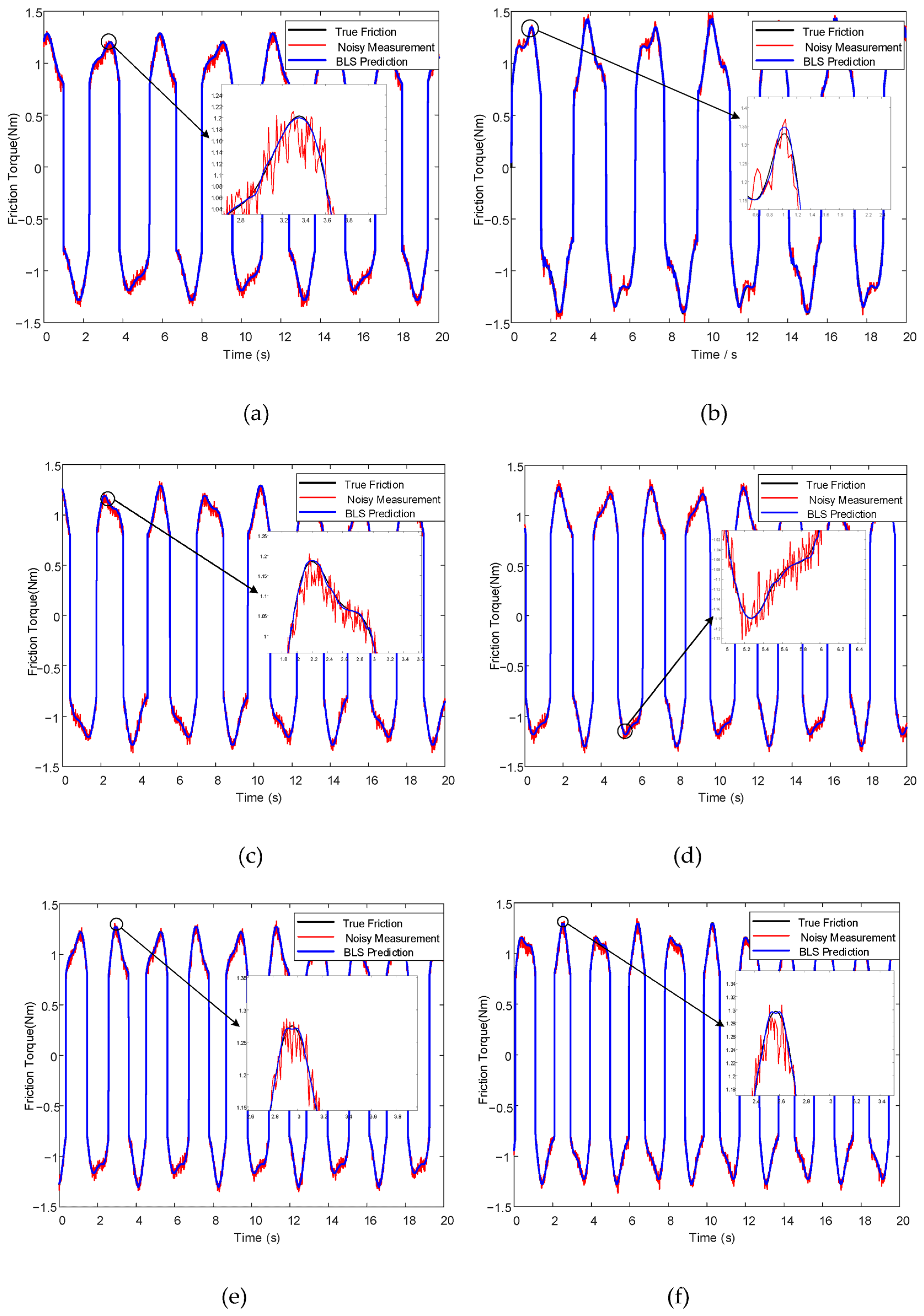
To better illustrate the prediction performance of the BLS model under noise interference, a local segment of the signal was magnified in Figure 6. The enlarged view clearly shows that, despite the presence of measurement noise, the BLS-predicted signal (blue curve) closely follows the true friction curve (black curve), demonstrating strong denoising capability and accurate fitting in transient regions.

The experimental results are shown in Figure 6. For each joint of the six-degree-of-freedom manipulator, the true friction torque and the predicted friction disturbance output by the BLS network were extracted and compared. This analysis verifies whether the BLS network can effectively filter out high-frequency noise and extract meaningful friction torque under actual control conditions, while also evaluating whether the prediction accuracy of the friction torque meets the requirements of the control system.

Figure 7a illustrates the torque prediction error for Joint 1. The error remains within ±0.008 N·m, with slight asymmetry. A peak deviation of +0.05 N·m occurs at the acceleration transition (t ≈ 2.1 s), while a negative peak of –0.06 N·m appears near the velocity reversal (t ≈ 8.7 s). During the steady motion phase (t = 4–7 s), the error stabilizes. These results confirm the BLS model’s ability to maintain continuity and dynamic responsiveness at motion inflection points.

Figure 7b illustrates the error pattern for Joint 2, showing periodic oscillations of ±0.018 N·m around t ≈ 3.5 s. The frequency corresponds to the second-order bending mode of the manipulator, indicating flexible coupling interference. Despite this, the BLS network constrains residual vibration energy effectively, demonstrating its suitability for flexible joint modeling and dynamic decoupling.

Figure 7c illustrates the error characteristics of Joint 3, with deviations consistently confined within ±0.015 N·m. Notable spikes occur at t ≈ 2.1 s and 8.7 s, aligned with nonlinear transitions in friction dynamics such as the Stribeck effect. The BLS framework accurately captures these nonlinearities while preserving overall convergence, reflecting strong sensitivity to hysteresis and transient dynamics.

Figure 7d illustrates the error of Joint 4, featuring higher-frequency fluctuations with the maximum amplitude reaching ±0.12 N·m. These oscillations likely arise from harmonic reducer meshing dynamics. Despite the challenging conditions, the PSO-tuned regularization parameter (λ = 1 × 10⁻⁴) ensures stable output and suppresses low-torque noise amplification, underscoring the model’s robustness.

Figure 7e illustrates the prediction error for Joint 5. The error signal is dense and irregular, with peaks near ±0.013 N·m, primarily concentrated in frequency bands associated with mechanical meshing. By applying a widened BLS structure with 20 enhancement nodes, the network successfully attenuates transient disturbances, validating its effectiveness in handling nonstationary structural noise.

Figure 7f illustrates the error profile for Joint 6, showing a composite signal of white noise with low-amplitude periodic components. The error remains stably bounded within ±0.015 N·m without significant drift. These features reflect the BLS model’s strong filtering capability under compound disturbances such as commutation noise and joint flexibility.

In conclusion, the proposed BLS-based friction modeling framework achieves consistently high torque prediction accuracy across all six joints. It demonstrates strong capability in handling nonlinear friction phenomena, flexible modal coupling, and dynamic noise interference. The model’s low error margins, robust convergence, and adaptability to multi-source disturbances highlight its potential for deployment in high-precision motion control and model-based predictive systems in advanced robotic applications.

4.2. Joint Total Torque Simulation Experiment

In vibration control, the dynamic accuracy of joint total torque is directly related to the positional stability of the end-effector. Therefore, to evaluate the ability of the proposed identification model to support control performance at the level of overall dynamic output, a joint total torque comparison simulation experiment was designed.

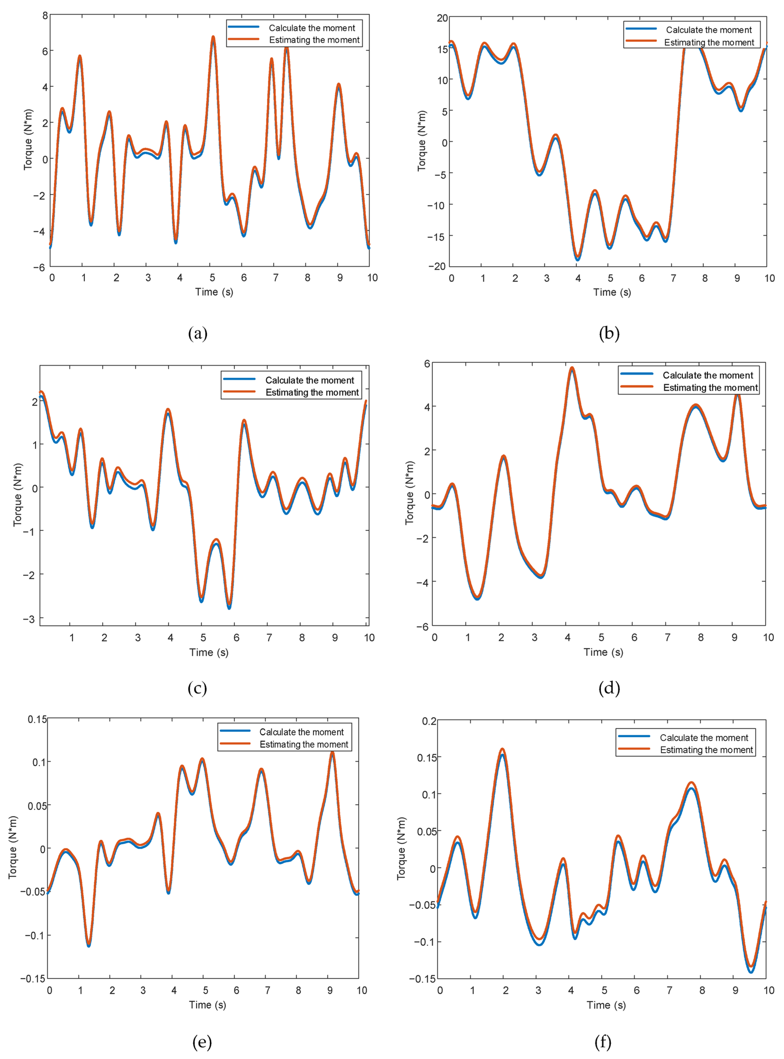
Figure 8 presents the comparison between the ideal total torque curves (blue lines) and the BLS-predicted total torque outputs (red lines) for all six joints.

As shown in Figure 8a, the two curves exhibit a high degree of overall alignment, with near-complete overlap in the main motion region (e.g., from t = 5 s to t = 10 s), indicating that the overall model effectively captures both the inertial and frictional characteristics of the system.

Minor deviations occur during the start-stop motion phases (around t = 0–2 s and t = 9–10 s), which can be attributed to abrupt coupling effects between system inertia and friction; this behavior falls within the expected scope of a standard identification model.

Figure 8b shows that the comparison curves for Joint 2 exhibit good overall performance. In particular, during the stable motion phase between 7 and 9 s, the predicted torque closely matches the ideal torque, demonstrating strong predictive capability.

Near the two prominent velocity reversal points (approximately at t = 4 s and t = 9 s), the predicted torque shows slight lag, with a maximum error of approximately 0.04 N·m. This is caused by the coupling between dynamic inertia variation and the nonstationary nature of friction characteristics. Such behavior is consistent with the inertial delay effects commonly observed in nonlinear dynamic system modeling and falls within a reasonable range.

In Figure 8c, the total torque comparison for Joint 3 exhibits more complex nonlinear characteristics. The predicted curve (blue line) generally follows the trend of the ideal curve (red line), but during several high-frequency motion phases (e.g., t = 7–10 s), noticeable fluctuations appear in the predicted torque.

These fluctuations are attributed to frequent velocity reversals and load changes in Joint 3, reflecting its complex coupled disturbance dynamics. Despite this, the overall prediction error remains within ±0.045 N·m, highlighting the model’s sensitivity to unstructured disturbances.

In Figure 8d, the torque prediction for Joint 4 appears exceptionally stable. Due to the lower intensity of nonlinear disturbances and the more consistent friction–inertia relationship of this joint, the two curves exhibit a very high degree of alignment. The overall error remains within ±0.02 N·m, with virtually no noticeable fluctuations.

Figure 8e shows that the total torque comparison for Joint 5 features clear high-frequency disturbance characteristics. The predicted curve generally follows the trend of the ideal curve throughout most of the motion cycle and performs particularly well during high-speed transition phases (e.g., around t = 6 s and t = 9 s). However, slight deviations are observed at certain local points (e.g., t = 3 s), with an amplitude of approximately 0.03 N·m.

For Joint 6, as illustrated in Figure 8f, the total torque prediction exhibits frequent disturbances and irregular fluctuations. While the predicted curve shows noticeable stochastic behavior, it closely matches the overall trend of the ideal total torque. The error is evenly distributed, and the maximum deviation remains below 0.02 N·m, demonstrating strong capability in tracking random disturbances.

4.3. Total Torque Error Analysis

To evaluate the accuracy of the identification model under vibratory conditions during motion, the total torque error is analyzed by comparing the true and predicted torques, with a focus on performance under vibration-induced excitation.

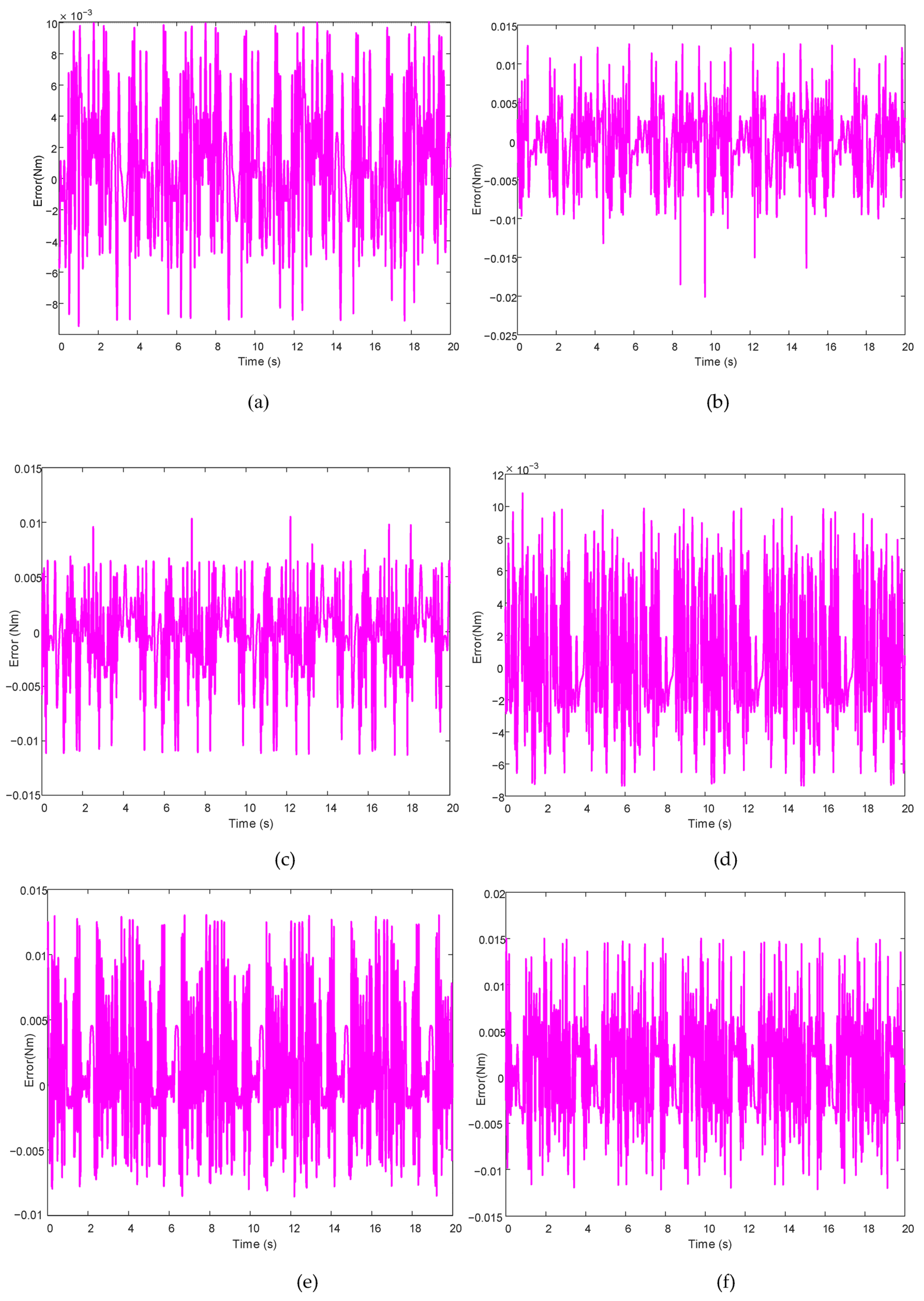
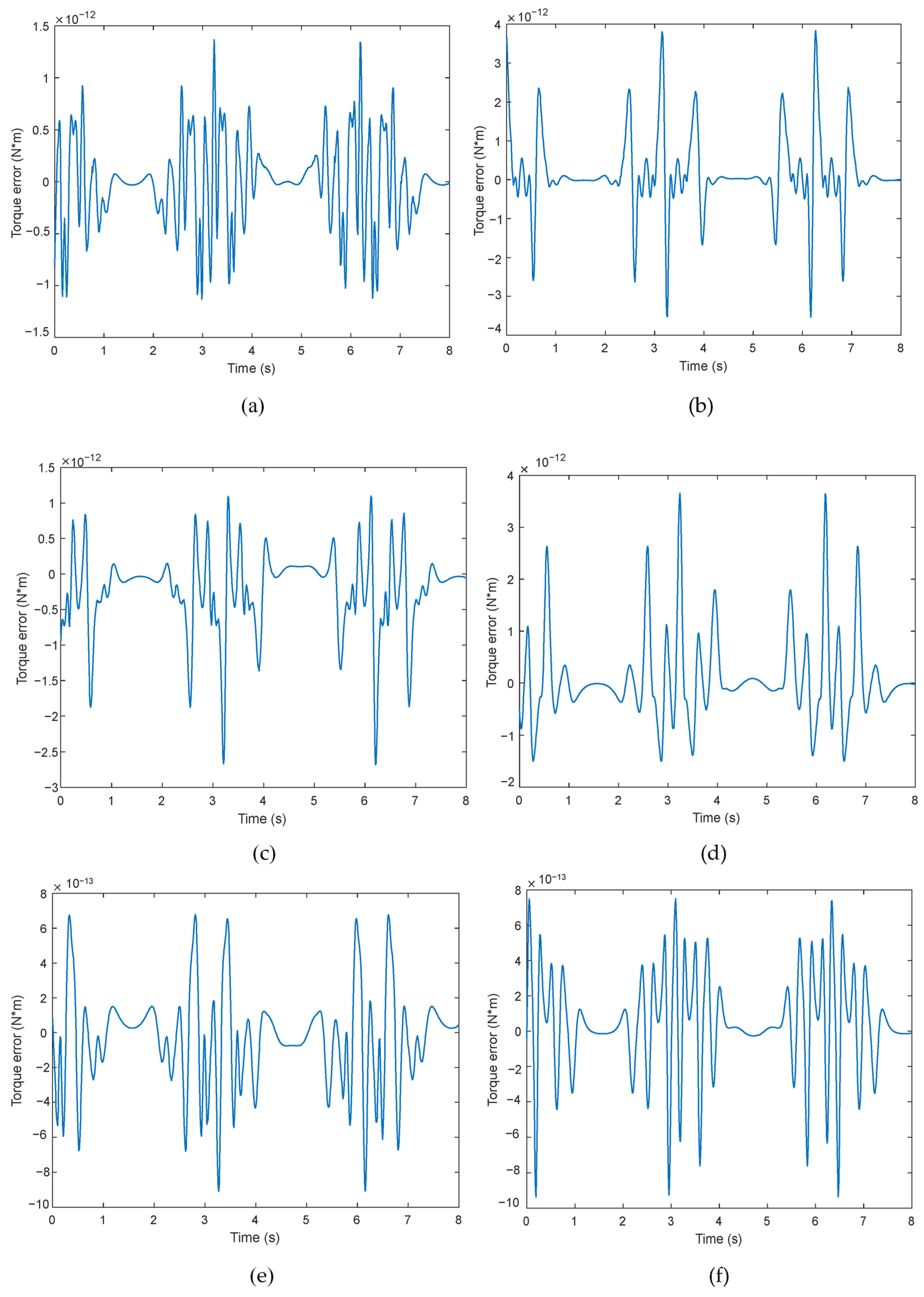
Figure 9 presents the total torque error curves for each joint. Figure 9a shows the prediction error for Joint 1. The error curve exhibits a generally random distribution, with a maximum deviation of less than 1.5 × 10⁻¹² N·m. Most of the error is concentrated around the start and end phases (0–1 s and 3–4 s), which correspond to dynamic transitions during manipulator start-up and stopping. In the steady-state motion phase (around 8 s), the error amplitude significantly decreases and approaches zero.

Figure 9b shows the identification error for Joint 2, with a maximum magnitude of approximately 4 × 10⁻¹² N·m. The error peaks are clearly located near the velocity reversal nodes (around 3 s and 6 s), corresponding to the nonlinear friction–inertia dynamic coupling points previously identified in the analysis. During the intermediate steady motion phase (4–5 s), the error fluctuations are minimal, with absolute values below 1 × 10⁻¹² N·m.

The total torque error curve for Joint 3, shown in Figure 9c, exhibits a certain degree of complexity and high-frequency oscillatory characteristics. The overall maximum error is approximately −2.5 × 10⁻¹² N·m, primarily concentrated in the time intervals of 3–4 s and 6–7 s.

These errors are associated with the frequent speed changes and strongly asymmetric frictional coupling characteristics of Joint 3. Nonetheless, the constructed model successfully keeps the error within a reasonable range, with the overall mean error remaining at a low and stable level.

The error curve for Joint 4 is shown in Figure 9d. The fluctuation amplitude is extremely low, remaining almost entirely within the range of ±4 × 10⁻¹² N·m throughout the motion. This joint is subject to relatively minimal nonlinear disturbances during the system identification process. Such performance is crucial for precision vibration suppression control strategies, as it effectively reduces the negative impact of micro-vibrations on end-effector positioning accuracy.

Figure 9e presents the total torque error curve for Joint 5, which exhibits typical high-frequency random disturbance characteristics. The maximum error amplitude is approximately 6 × 10⁻¹² N·m, mainly concentrated in the frequently varying velocity regions between 2–4 s and 6–7 s.

As discussed earlier, these errors correspond to the high-frequency components of friction torque coupled with nonlinear disturbances from inertial load variation. Overall, the model keeps the error within a relatively small range and demonstrates strong adaptability to high-frequency disturbances and load fluctuations.

Figure 9f shows the error curve for Joint 6. Due to the lower inertia of the end-effector degree of freedom, this joint is more sensitive to frictional noise, resulting in slightly larger errors compared to the previous joints. The maximum error amplitude is around ±8 × 10⁻¹² N·m.

Nevertheless, the friction modeling network effectively suppresses the influence of high-frequency noise, keeping the overall error stable and within a controlled range. These results further confirm the model’s capability for high-precision, small-disturbance capture, making it suitable for robotic manipulator micro-vibration suppression scenarios.

4.4. Comparative Analysis

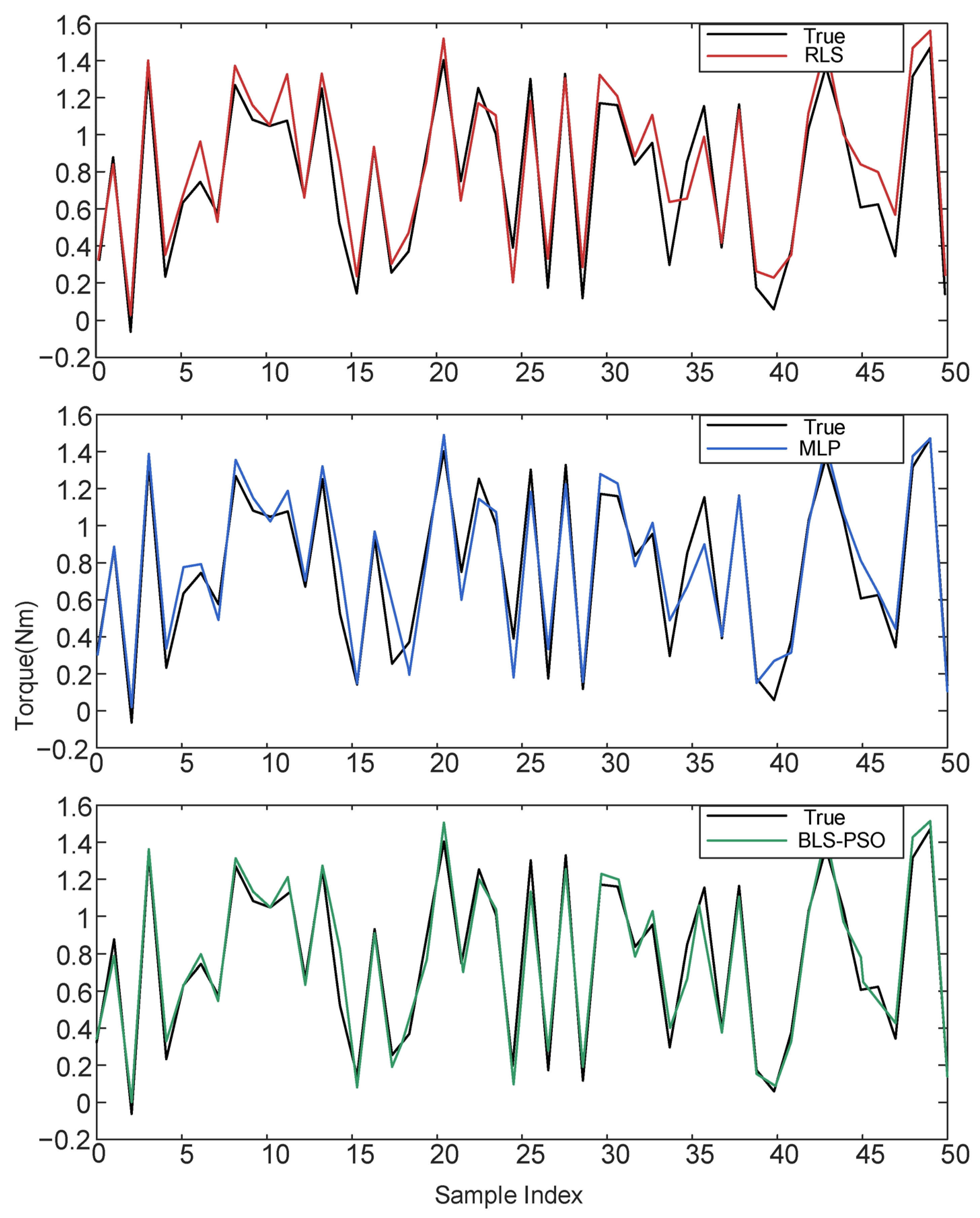
To comparatively evaluate the torque prediction performance of different modeling methods, three representative approaches—RLS, MLP, and the proposed BLS-PSO—are illustrated in Figure 10. From top to bottom, the subplots correspond to RLS, MLP, and BLS-PSO predictions versus the ground truth.

RLS (Top): Although the Recursive Least Squares (RLS) method captures the general trend of the torque curve, it exhibits noticeable deviations in regions with sharp fluctuations. This indicates limited adaptability to the nonlinear and non-smooth characteristics of the friction torque.

MLP (Middle): The Multi-Layer Perceptron (MLP) achieves better performance than RLS in capturing the high-frequency variations. However, it still suffers from overshooting and irregular fitting in certain regions, especially when the signal is noisy or dynamically changing.

BLS-PSO (Bottom): In contrast, the proposed BLS-PSO method demonstrates significantly improved prediction accuracy, with its output curve closely tracking the true torque across the entire sample index range. The alignment between the green prediction line and the black ground truth curve is notably tighter, validating the effectiveness of combining Broad Learning with PSO-based adaptive optimization in handling nonlinearity and model uncertainty.

This comparative result highlights the superior generalization and noise robustness of the proposed method, making it a more suitable choice for real-time robotic torque modeling applications.

As shown in Figure 11, the proposed BLS-PSO method yields consistently smaller prediction errors across the test samples. Compared to RLS and MLP, BLS-PSO demonstrates improved stability and reduced peak deviations, particularly in mid and late test intervals. The results validate its capability to accurately capture nonlinear dynamics and suppress modeling noise.

Table 2. Quantitative comparison of three methods.

Method	RMSE	Smoothness	Time
RLS	0.11723	0.60058	0.0001024
MLP	0.11116	0.56249	0.044911
BLS-PSO	0.10893	0.55865	0.0003557

summarizes the numerical results of the three evaluated methods. The proposed BLS-PSO achieves the lowest RMSE (0.10893) and highest smoothness (0.55865), indicating superior prediction accuracy and reduced output vibration. Although its computation time (0.00036 s) is slightly higher than RLS, it remains significantly faster than MLP. The results confirm that BLS-PSO offers the best trade-off among accuracy, robustness, and efficiency, making it well suited for real-time robotic applications.

5. Conclusions

This study proposes a dynamic parameter identification method for robotic manipulators based on the integration of BLS and PSO. By combining this approach with a zero-boundary fifth-order Fourier excitation trajectory, the method achieves high-precision modeling of both the system’s structural dynamics and nonlinear frictional disturbances, ultimately serving vibration suppression control.

Simulation results demonstrate that the proposed method maintains low total torque prediction errors across various representative motion scenarios. It effectively captures complex joint-specific friction characteristics and unstructured disturbance dynamics, validating its effectiveness and generalizability in both complex mechanical system identification and practical engineering applications. Furthermore, the hybrid modeling framework improves data utilization efficiency, enabling accurate parameter identification even under limited or constrained data conditions, which is critical for real-time robotic control environments.

In future work, this identification method can be further integrated into actual control loops to explore its capabilities in vibration source separation modeling and feed forward disturbance rejection control under strongly nonlinear and flexible structural conditions, with the goal of developing adaptive vibration suppression systems with learning capabilities.