Capturing User Preferences via Multi-Perspective Hypergraphs with Contrastive Learning for Next-Location Prediction

Abstract

With the widespread adoption of mobile devices and the increasing availability of user trajectory data, accurately predicting the next location a user will visit has become a pivotal task in location-based services. Despite recent progress, existing methods often fail to effectively disentangle the diverse and entangled behavioral signals, such as collaborative user preferences, global transition mobility patterns, and geographical influences, embedded in user trajectories. To address these challenges, we propose a novel framework named Multi-Perspective Hypergraphs with Contrastive Learning (MPHCL), which explicitly captures and disentangles user preferences from three complementary perspectives. Specifically, MPHCL constructs a global transition flow graph and two specialized hypergraphs: a collective preference hypergraph to model collaborative check-in behavior and a geospatial-context hypergraph to reflect geographical proximity relationships. A unified hypergraph representation learning network is developed to preserve semantic independence across views through a dual propagation mechanism. Furthermore, we introduce a cross-view contrastive learning strategy that aligns multi-perspective embeddings by maximizing agreement between corresponding user and location representations across views while enhancing discriminability through negative sampling. Extensive experiments conducted on two real-world datasets demonstrate that MPHCL consistently outperforms state-of-the-art baselines. These results validate the effectiveness of our multi-perspective learning paradigm for next-location prediction.

1. Introduction

With the widespread adoption of location-based services and the increasing availability of user mobility data, location prediction [1,2,3]—the task of forecasting the future position a user is likely to visit based on their historical movement trajectory—has gained significant attention in recent years. It plays a critical role in various real-world applications such as personalized recommendation systems [4], intelligent navigation [5], urban planning [6], and location-aware advertising [7]. 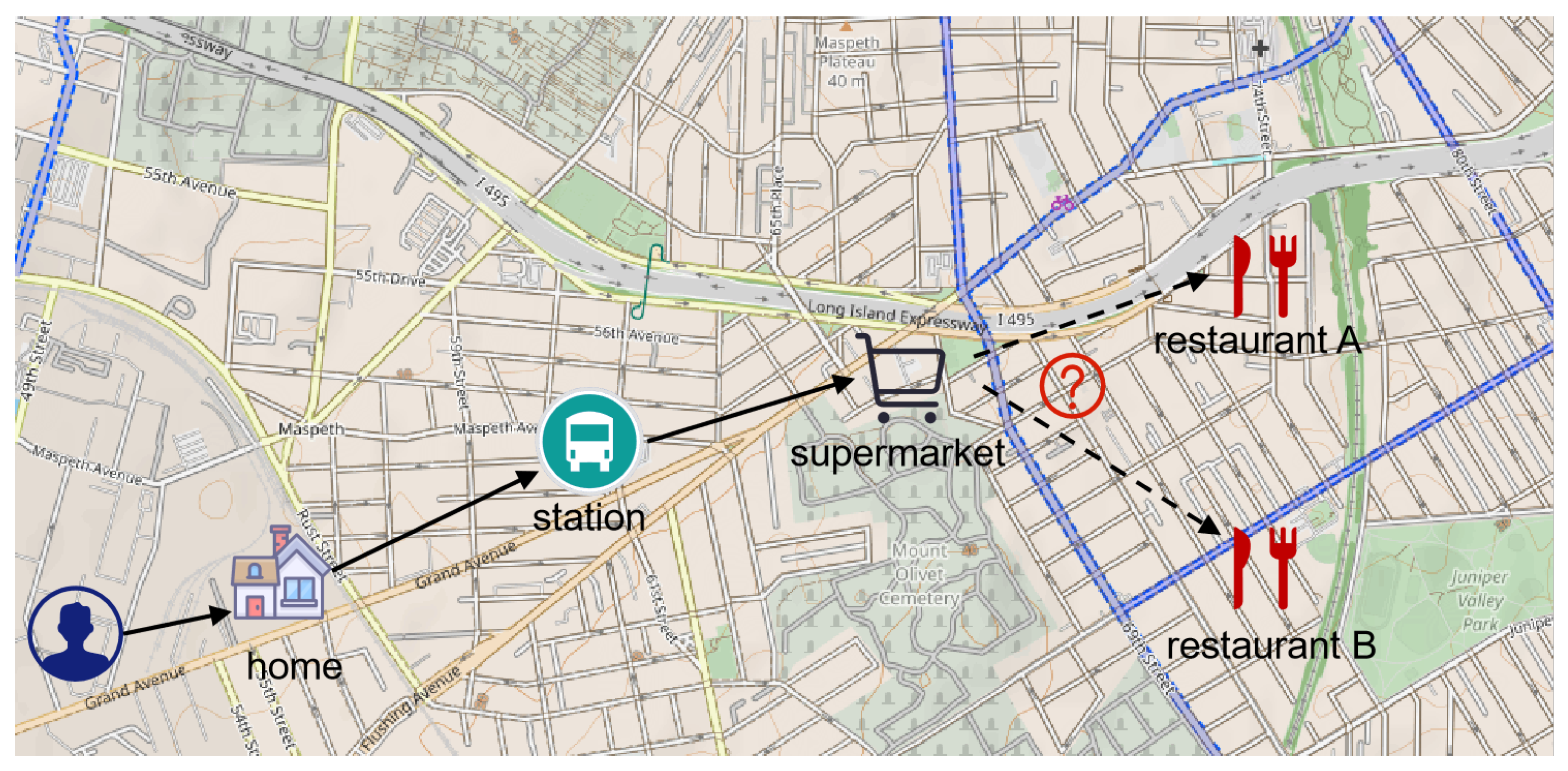In many studies, the location prediction is also referred to as a point-of-interest (POI) recommendation, where a POI denotes specific geographical entities like restaurants, parks, or stores that users may check into and visit, as shown in Figure 1. It aims to infer user preferences and contextual patterns from historical trajectory data and predict which location predictions users are most likely to visit next. Location prediction addresses the fundamental problem: leveraging users’ spatiotemporal behavioral history to anticipate their next geographical action.

Numerous models have been developed to address this task, which can broadly be categorized into four main groups. The first group comprises traditional approaches such as collaborative filtering (CF) [8,9] and matrix factorization (MF) [10,11], which capture co-visitation or preference patterns but often struggle with sequential or spatial dynamics. The second category includes recurrent neural network (RNN)-based models [12,13,14,15], which utilize temporal sequence modeling to learn the evolution of user preferences over time. However, these models often face limitations in capturing long-term dependencies and complex spatial interactions. The third group introduces attention-based models [16,17,18,19] that dynamically assign weights to different historical check-ins or contextual factors, improving the ability to model user intent. Finally, graph-based [20,21,22] and hypergraph-based methods [23,24,25] have emerged as powerful tools for modeling high-order and non-Euclidean user-location prediction relationships by representing check-in sequences and spatial clusters as graphs or hypergraphs. These approaches offer enhanced flexibility in representing multifaceted interactions but still face challenges in disentangling diverse behavioral influences effectively. In recent studies, contrastive learning has also been coupled with advanced probabilistic methods such as Variational Bayes [26]. These methods provide a robust framework for sparse recovery, enabling more efficient learning in high-dimensional spaces.

Despite the substantial advancements in location prediction, three critical challenges remain unresolved, limiting the effectiveness of current models:

First, a prevalent limitation lies in the entanglement of heterogeneous behavioral signals—such as collective user preferences, sequential transition patterns, and geographical proximity—into a unified latent representation. This monolithic embedding often obscures the distinct contribution of each factor, making it difficult to interpret the underlying decision-making process and reducing the model’s ability to adapt to varying user behaviors across contexts.

Second, although some recent approaches [27,28,29] leverage graph-based or multi-relational structures to capture diverse interaction patterns, they frequently fall short in terms of explicit disentanglement. Instead of modeling each behavioral perspective independently, these models often integrate multiple views into a single graph structure or latent space without clearly separating their semantic roles. As a result, the learned representations tend to be entangled and coarse-grained, which hampers the model’s ability to capture fine-grained, view-specific dynamics essential for accurate location prediction.

Third, even in models [30,31] that do acknowledge multiple views, there is a notable lack of mechanisms for explicit alignment or contrastive integration across these perspectives. Without encouraging consistency or highlighting distinctions among views, the model fails to fully exploit the complementary nature of multi-perspective information. This deficiency becomes especially pronounced in scenarios characterized by data sparsity and noisy check-in records, where robust and discriminative representations are crucial for generalization. Consequently, the inability to systematically disentangle and reconcile different behavioral signals remains a bottleneck in achieving accurate location predictions.

To address the above challenges in location prediction, we propose a novel framework named Multi-Perspective Hypergraphs with Contrastive Learning (MPHCL), which captures and disentangles user preferences by integrating three key behavioral dimensions. The framework comprises three individual graphs: (1) the collective preference hypergraph for collaborative preferences within the user community, (2) the geospatial context hypergraph for spatial correlations between locations, and (3) the global transition flow graph for mobility patterns based on visit sequences. This multi-perspective approach enables nuanced disentanglement of behavioral factors influencing user mobility. We introduce a unified hypergraph representation learning network that ensures the independence of each perspective during embedding, utilizing a node–hyperedge–node message passing framework and across-hyperedge propagation to prevent feature entanglement. Additionally, a cross-view contrastive learning mechanism aligns multi-view representations by treating embeddings of the same user or location across different views as positive pairs while considering others as negative. This approach enhances consistency, strengthens the robustness of learned embeddings, especially under sparse or noisy data, and facilitates effective integration of diverse signals. Consequently, MPHCL provides a comprehensive and personalized understanding of user intent, leading to improved performance in location prediction tasks.

In short, our main contributions are summarized as follows:

• We propose a novel Multi-Perspective Hypergraphs with Contrastive Learning (MPHCL) model for location prediction, which disentangles user preferences by leveraging hypergraphs from three perspectives. Our unified hypergraph representation learning network incorporates a two-step information propagation scheme to capture high-order locations, including within-hyperedge feature aggregation and across-hyperedge feature propagation. Additionally, we introduce a cross-view contrastive learning mechanism that enhances view-specific user and location prediction representations through self-supervised signals.
• We leverage graph Laplacian matrices to perform effective spectral reasoning over the constructed hypergraphs, which allows for the propagation of user preferences along directed paths in the process of graph learning.
• Extensive experiments on two real-world datasets have verified the prediction performance of our proposed MPHCL model compared with various state-of-the-art methods.

2. Related Work

Next-location prediction has become a fundamental task in location-based services, prompting the development of various predictive models. Existing methods can be broadly classified into four categories: traditional approaches, recurrent neural network-based models, attention-enhanced sequential frameworks, and graph-based techniques. In this section, we review representative works from each category and discuss their respective strengths and limitations.

2.1. Traditional Approaches

Traditional methods such as collaborative filtering (CF) [8,9] and matrix factorization (MF) [10,11] have long served as foundational techniques in location-based social network (LBSN) recommendations. CF-based approaches typically model user preferences by leveraging behavioral similarities among users or items. For instance, Lian et al. [8] integrate short-term sequential transitions and long-term personalized preferences through a latent factor model, effectively capturing spatio-temporal dynamics and individualized patterns for next-location prediction. Meanwhile, the ICCF model [9] enhances CF by incorporating semantic features and implicit feedback, utilizing a confidence-weighted framework to mitigate cold-start challenges and extract meaningful patterns from heterogeneous data sources such as user demographics and textual content. On the other hand, MF-based methods aim to decompose the user-item interaction matrix into low-rank latent spaces. GeoMF++ [10] introduces spatially aware latent factors through grid-based modeling to jointly learn user preferences and geographical influences, demonstrating strong scalability and robustness to sparsity. Similarly, SQPMF [11] unifies social trust, transition behaviors, and personalized preferences within a probabilistic matrix factorization model, leveraging contextual and sequential cues to enhance location prediction accuracy. Despite their effectiveness, these traditional approaches often struggle with modeling complex higher-order relationships and disentangling multifaceted user intents, motivating the development of more advanced representation learning techniques.

While some traditional trip choice models (e.g., discrete choice models, gravity models, and agent-based simulations) typically rely on predefined utility functions and require extensive feature engineering or domain-specific priors, our method is data-driven and leverages graph-based representation learning with self-supervised contrastive signals. Moreover, unlike transport system models (TSMs) [32,33] that focus on macroscopic travel flows, our model aims at personalized, fine-grained next-location prediction in location-based social networks (LBSNs), which emphasizes individual behavioral signals, rather than aggregate transportation flows.

2.2. RNN-Based Models

To capture the sequential dependencies inherent to user mobility patterns, recurrent neural network (RNN)-based models have been widely adopted for next-location prediction. Early RNN variants, such as ST-RNN [12], incorporate temporal and spatial intervals into standard RNN architectures, enabling the modeling of time-aware and location-sensitive user trajectories. To further address the challenge of heterogeneous user preferences, GTSAR-RNN [13] introduces a group-specific modeling strategy, where users are clustered via probabilistic matrix factorization, and separate RNNs are trained to capture intra-group behavioral dynamics. By integrating sentiment-aware location prediction aspects, geographical categories, and temporal context, this model significantly enhances personalization and relevance, especially under sparse data conditions. More recent approaches, such as NeuNext [14], enhance traditional LSTM networks with specialized time and distance gates, effectively capturing both short-term transitions and long-term interests through adaptive spatio-temporal gating mechanisms. Meanwhile, LSTPM [15] advances sequential modeling by combining geo-dilated LSTMs with a nonlocal attention mechanism, allowing the model to simultaneously attend to long-range dependencies and local contextual cues. Despite their notable success in modeling sequential behaviors, RNN-based methods often struggle to represent high-order or multi-relational structures among users and location predictions, limiting their expressiveness in capturing complex spatial or collaborative influences embedded in real-world check-in data. These models primarily focus on pairwise relationships, which makes it difficult to capture complex interactions that involve multiple users or locations simultaneously. As a result, RNNs struggle to model collaborative co-visitation patterns, spatial dependencies between locations, and other higher-order relationships that are crucial for accurate location prediction.

2.3. Attention-Based Models

Attention-based models have emerged as a powerful alternative to traditional sequential methods to better capture user intent and contextual nuances. These approaches assign dynamic weights to historical check-ins and contextual signals, thereby enhancing the interpretability and adaptability of location prediction. STAN [16] employs a bi-layer spatiotemporal attention mechanism to model temporal dependencies and geographical proximity while incorporating personalized item frequency to account for repetitive behavioral patterns. Extending this idea, GETNext [17] constructs a global trajectory flow map and uses graph convolutional layers to integrate spatial, categorical, and temporal properties, offering a holistic representation of user mobility dynamics. More advanced models like Diff-DGMN [18] fuse dual-graph learning with diffusion-based sampling to jointly model user-specific sequential transitions and global location prediction spatial distributions. Its directional attention and stochastic reverse process allow for effective preference generation even under cold-start conditions. Similarly, ImNext [19] addresses the challenges of unstructured spatiotemporal gaps and multitask learning by combining self-attention mechanisms with robust trajectory modeling, outperforming various baselines across diverse urban datasets. While attention-based models demonstrate strong capability in capturing salient features from complex mobility data, they often treat user behaviors as flat sequences or rely on pairwise relations, lacking an explicit mechanism to disentangle diverse interaction signals such as collaborative preferences, temporal transitions, and geographic proximity in a unified framework.

2.4. Graph-Based and Hypergraph-Based Methods

Graph-based and hypergraph-based methods have gained increasing attention in location prediction due to their ability to model high-order and non-Euclidean interactions among users and locations. Zuo et al. [20] construct multi-view graphs—including global location prediction feature and distance graphs, as well as user-specific historical graphs—to jointly capture long-term preferences and spatial constraints through the fusion of GCN and Transformer architectures. Similarly, Graph-Flashback [21] builds a spatial-temporal knowledge graph (STKG) to encode weighted location prediction transition patterns, employing GCNs and personalized similarity functions to refine sequential representations and enhance user-specific modeling. To further enrich relational semantics, HKGNN [22] leverages hyper-relational knowledge graphs by integrating user-location prediction-time mobility patterns, social ties, and location prediction attributes into a unified hypergraph structure. It combines a hypergraph neural network with attention-based encoders and decoders to capture complex structural and contextual dependencies, yielding robust performance under data sparsity.

Hypergraph-based models extend beyond conventional pairwise graphs by modeling multi-entity interactions as hyperedges. DHCL [23] constructed hypergraphs with three different perspectives to decouple and represent user preferences. MSTHN [24] constructs an enhanced spatial–temporal hypergraph that captures both local sequential dependencies and global collaborative signals, applying a dual-level aggregation strategy to adaptively represent dynamic user behaviors. STHGCN [25] also adopts a hypergraph approach, aggregating multi-hop spatiotemporal trajectory information to better model complex check-in patterns. While these methods demonstrate strong capabilities in modeling structural relationships, most do not explicitly disentangle the diverse behavioral factors, such as collaborative co-visitation, sequential mobility, and geographic proximity, into independent representations, potentially limiting generalization. In contrast, our proposed framework addresses this gap through multi-perspective hypergraph construction and contrastive disentanglement.

While traditional collaborative filtering and matrix factorization methods offer foundational insights into user-location preferences, and RNN and attention-based models advance sequential and contextual modeling, they often fall short in capturing complex, high-order, and multi-relational dynamics. Graph and hypergraph-based approaches have further pushed the boundaries by modeling structured interactions and high-order associations, yet most existing models still entangle heterogeneous behavioral signals into unified latent spaces, hindering adaptability. Motivated by these limitations, our work proposes a novel framework that explicitly disentangles user preferences from collaborative, sequential, and geographical perspectives using multi-perspective hypergraphs and contrastive learning, thereby enabling more robust and personalized location prediction.

3. Preliminaries

3.1. Task Formulation

Let $U=\{u_1,u_2,\dots ,u_{\left|U\right|}\}$ denote a set of users and $L=\{l_1,l_2,\dots ,l_{\left|L\right|}\}$ represent a collection of locations. Every location, $l\in L$, is characterized by a distinct geographical coordinate tuple, specifically defined as (longitude, latitude), i.e., $(lon,lat)$. For each user $u\in U$, we extract their trajectory represented as ${\mathcal{S}}_u=\left\{(l_i,t_i)\right\}\mid i=1,2,\dots ,n\}$, wherein each tuple $(l_i,t_i)$ signifies that user u visited location $l_i$ at the corresponding timestamp, $t_i$.

Considering a specified user, u, along with their trajectory sequence, ${\mathcal{S}}_u$, the primary objective of the location prediction task is to predict top-k locations that user u is anticipated to visit in the next timestamp.

3.2. Hypergraph

A hypergraph is a generalized structure of a graph [34], where a single edge can connect two or more vertices simultaneously, thereby allowing for more complex relationships among the vertices. An example is shown in Figure 2. Formally, a hypergraph can be denoted as $\mathcal{G}=\{\mathcal{V},\mathcal{E},\mathbf{H}\}$, where $\mathcal{V}$ represents the set of vertices and $\mathcal{E}$ denotes the collection of hyperedges. To effectively capture the topological arrangement of vertices and hyperedges within this framework, the incidence matrix can be introduced, represented as $\mathbf{H}\in {\mathbb{R}}^{\left|\mathcal{V}\right|\times \left|\mathcal{E}\right|}$. This matrix serves as a critical tool in the analysis of hypergraphs; specifically, when a vertex, $v\in \mathcal{V}$, is included in a hyperedge, $e\in \mathcal{E}$, the corresponding entry in the incidence matrix is defined as $\mathbf{H}(v,e)=1$; otherwise, it is set to $\mathbf{H}(v,e)=0$. This binary representation allows for a concise depiction of the interconnections among vertices and hyperedges, facilitating the further exploration of the hypergraph’s properties and applications.

4. Methodology

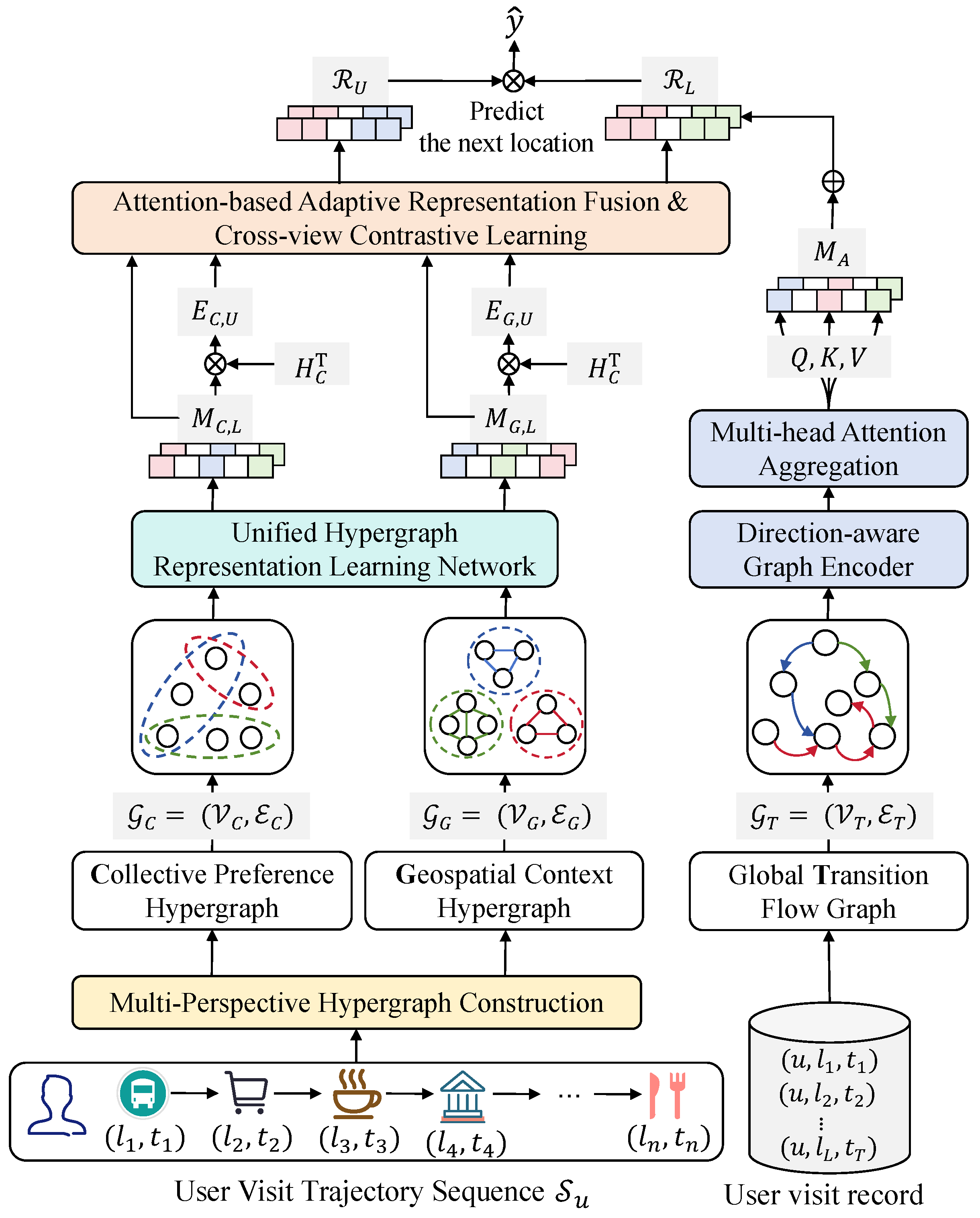
The overall framework of the proposed Multi-Perspective Hypergraphs with Contrastive Learning (MPHCL) model for location prediction is illustrated in Figure 3. The collective preference hypergraph captures collaborative user behavior, the geospatial context hypergraph reflects the spatial relationships between locations, and the global transition flow graph models the sequential dependencies in user visits. The model employs a two-step information propagation mechanism to capture high-order dependencies within each hypergraph. Additionally, the cross-view contrastive learning module aligns the embeddings from different views, maximizing agreement across user and location representations. This architecture enables the model to integrate complementary information from multiple perspectives for more accurate location predictions.

4.1. Multi-Perspective Hypergraph Construction

In the realm of location prediction, understanding the intricate interaction relationships between users and locations is paramount. These relationships are multifaceted, encompassing (1) user-location interactions, (2) transitional dynamics that reflect the relationships among different locations, and (3) geographical correlations that emerge from the physical proximity of these locations. To capture and model these complex dynamics effectively, previous studies have introduced methodologies that treat users and locations as discrete nodes within a graph framework, wherein the interconnections between them are represented as edges.

However, traditional graph structures involve notable limitations [35], as they predominantly focus on pairwise relationships. This approach restricts the ability to capture higher-order interactions, i.e., those that involve multiple nodes concurrently, which are often crucial for understanding the underlying semantic context. For instance, the social dynamics surrounding a user’s engagement with multiple locations or the interrelationships among a cluster of geographically proximate locations may involve intricate interactions that a conventional graph representation cannot adequately express.

Given these constraints, we recognize the necessity of a more sophisticated framework that can accommodate the complexities of these relationships. Inspired by the highly flexible and versatile nature of hypergraphs [36], we propose a novel approach that entails the design of three distinct hypergraphs. These hypergraphs are not merely enhancements of traditional structures but, rather, represent a paradigm shift in how we conceptualize relational data within the location prediction sphere. Each hypergraph is meticulously crafted to encapsulate different aspects of user–location interactions, thereby facilitating a richer representation of the relational patterns.

4.1.1. Collective Preference Hypergraph

In order to effectively capture the high-order interactions between users and locations, we construct a collective preference hypergraph, ${\mathcal{G}}_C=({\mathcal{V}}_C,{\mathcal{E}}_C,{\mathbf{H}}_C,{\mathbf{W}}_C)$, where ${\mathcal{V}}_C=\{l_1,l_2,\dots ,l_{\left|L\right|}\}$ denotes the set of locations, and ${\mathcal{E}}_C=\{e_u\mid u\in U\}$ represents the collection of user-specific trajectories encoded as hyperedges. Each hyperedge, $e_u\subseteq {\mathcal{E}}_C$, comprises the locations visited by user u and is weighted by a diagonal matrix ${\mathbf{W}}_C=\mathrm{diag}(w_1,\dots ,w_{\left|U\right|})$, where each hyperedge weight, $w_u=1/|e_u|$, provides trajectory length normalization to counterbalance varying visitation frequencies. Hyperedges are formed based on the check-in trajectories of individual users. Specifically, each user’s visit history is represented as a hyperedge, where each hyperedge connects the locations that the user has visited. These hyperedges are weighted by the length of the user’s trajectory to normalize the visitation frequencies, ensuring that users with more frequent visits do not dominate the learning process. The user-location visit pattern is encoded by the incidence matrix ${\mathbf{H}}_C\in {\{0,1\}}^{\left|L\right|\times \left|U\right|}$, with elements defined as follows:

$$H_C(l,e_u)=\left\{\begin{array}{cc}1,\hfill & \mathrm{if}l\in e_u\hfill \\ 0,\hfill & \mathrm{otherwise}\hfill \end{array}\right.$$

(1)

The vertex degrees are computed as $d\left(v\right)={\sum }_{e_u\in {\mathcal{E}}_C}{\mathbf{H}}_C(v,e_u)·w_u$, while the hyperedge degrees are given by $\delta \left(e_u\right)={\sum }_{v\in {\mathcal{V}}_C}{\mathbf{H}}_C(v,e_u)$, forming diagonal degree matrices ${\mathbf{D}}_v\in {\mathbb{R}}^{\left|L\right|\times \left|L\right|}$ and ${\mathbf{D}}_e\in {\mathbb{R}}^{\left|U\right|\times \left|U\right|}$.

The intra-sequence co-visitation structure is captured by the weighted adjacency matrix ${\mathbf{H}}_C{\mathbf{W}}_C{\mathbf{H}}_C^{\top }$, which encodes the relational strength between locations. To capture inter-sequence user dependencies based on shared location visitation, we define a hyperedge similarity metric using cosine similarity as follows:

$$\mathrm{Sim}(u_i,u_j)={\displaystyle \frac{|{\mathbf{H}}_C{(:,e_{u_i})}^{\top }{\mathbf{H}}_C(:,e_{u_j})|}{\parallel {\mathbf{H}}_C(:,e_{u_i})\parallel ·\parallel {\mathbf{H}}_C(:,e_{u_j})\parallel }},$$

(2)

where ${\mathbf{H}}_C(:,e_u)$ denotes the column of ${\mathbf{H}}_C$ corresponding to hyperedge $e_u$.

Information propagation over the collective preference hypergraph is governed by the hypergraph Laplacian ${\mathbf{L}}_C={\mathbf{D}}_v-{\mathbf{H}}_C{\mathbf{W}}_C{\mathbf{D}}_e^{-1}{\mathbf{H}}_C^{\top }$, enabling the learning of diffusion-aware representations. Furthermore, a spectral analysis of the kernel ${\mathbf{H}}_C{\mathbf{W}}_C^{1/2}{\mathbf{D}}_e^{-1}{\mathbf{W}}_C^{1/2}{\mathbf{H}}_C^{\top }$ allows for the identification of latent user clusters exhibiting similar behavioral patterns across the location space. The proposed collective preference hypergraph ${\mathcal{G}}_C$ facilitates the modeling of both local user trajectory structures and global co-visitation patterns.

4.1.2. Geospatial Context Hypergraph

The construction of the geographical view hypergraph is a sophisticated process that entails the formulation of a hypergraph designed to represent the geographical relationships among different locations while adhering to specific spatial constraints. Formally, we denote a geospatial context hypergraph as ${\mathcal{G}}_G=({\mathcal{V}}_G,{\mathcal{E}}_G,{\mathbf{H}}_G,{\mathbf{W}}_G)$, where ${\mathcal{V}}_G$ represents the set of locations. Locations that are within a predefined distance threshold, calculated using the Haversine distance, are connected via hyperedges. These hyperedges capture the spatial relationships between geographically close locations, reflecting the proximity effect in user preferences. Within this hypergraph ${\mathcal{G}}_G$, a hyperedge is established to connect locations that lie within a predetermined distance threshold ${\mathrm{\Delta }}_d$. This threshold is critical for accurately capturing the proximity of interactions and is derived from the Haversine distance metric $d_H$, which is mathematically expressed as follows:

$$d_H(l_i,l_j)=2R·arcsin\left(\sqrt{{sin}^2\left({\displaystyle \frac{{\varphi }_i-{\varphi }_j}{2}}\right)+cos\left({\varphi }_i\right)cos\left({\varphi }_j\right){sin}^2\left({\displaystyle \frac{{\lambda }_i-{\lambda }_j}{2}}\right)}\right),$$

(3)

where $(l_i,l_j)$ represents two locations, $({\varphi }_i,{\varphi }_j)$ denotes latitudes of locations $(l_i,l_j)$, $({\lambda }_i,{\lambda }_j)$ signifies longitudes of locations $(l_i,l_j)$, and $R=6371 \mathrm{km}$ is the Earth’s radius.

In our model, we utilize the Haversine distance metric to capture geographical proximity between locations, as it accurately accounts for the curvature of the Earth. Unlike the Euclidean norm, which assumes a flat plane and is suitable only for small-scale distances, the Haversine distance calculates the shortest path along the surface of a sphere, making it ideal for modeling real-world spatial relationships between locations. This ensures that the proximity relationships between locations are represented more realistically, especially for large geographical areas.

Consequently, the incidence matrix ${\mathbf{H}}_G\in {\mathbb{R}}^{\left|\mathcal{L}\right|\times |{\mathcal{E}}_G|}$ serves as a crucial role in depicting the geographical interactions among locations. Specifically, if the Haversine distance between $l_i$ and $l_j$ satisfies the condition $d_H(l_i,l_j)\le {\mathrm{\Delta }}_d$, we designate ${\mathbf{H}}_G(i,j)=1$. Conversely, if the distance exceeds the threshold, we set ${\mathbf{H}}_G(i,j)=0$. This binary representation encapsulates the existence of geographical relationships and enables the exploration of patterns in spatial clustering that significantly influence user behaviors and preferences.

The proposed geospatial context hypergraph ${\mathcal{G}}_G$ is not merely a mathematical construct, and it embodies critical geographical influences that play a vital role in shaping user preferences in real-world contexts. By integrating this spatial dimension, we can elucidate how users traverse their environments, uncovering visitation patterns often dictated by geographical proximity. This structure thus effectively reflects user geographical preferences, allowing us to analyze how proximity impacts user decision-making processes when selecting the next locations.

So far, we have constructed two hypergraphs from diverse perspectives, namely the collective preference hypergraph ${\mathcal{G}}_C$ and the geospatial context hypergraph ${\mathcal{G}}_G$. Next, we will propose a disentangled hypergraph representation learning network to explicitly model and derive enriched representations of locations. Employing a disentangled learning framework, we can isolate the contributions of each viewpoint, facilitating a comprehensive understanding of user dynamic visit preferences.

4.2. Global Transition Flow Graph

While traditional hypergraphs can effectively capture high-order and undirected associations among entities, they are inherently limited in representing directional semantics, such as location-to-location transitions in user visit trajectories. In contrast to the collective preference hypergraph, which models co-visitation, we define a Global Transition Flow Graph ${\mathcal{G}}_T=({\mathcal{V}}_T,{\mathcal{E}}_T,{\mathbf{H}}_T,{\mathbf{W}}_T)$ to encode directed transition dynamics between locations. Here, the vertex set ${\mathcal{V}}_T=\{l_1,l_2,\dots ,l_{\left|L\right|}\}$ denotes the set of locations, while the edge set ${\mathcal{E}}_T=\{e_u^T\mid u\in U\}$ captures the sequential transitions observed in all user visit records, where each $e_u^T$ corresponds to an ordered set of location transitions $(l_i\to l_j)$ made by user u. Hyperedges represent transitions between locations based on sequential visit data. Each hyperedge in this graph connects a pair of locations, representing the direct transitions from one location to another in a user’s trajectory. These transitions are directed to preserve the movement dynamics of users. To represent such directional transitions, we define the incidence matrix ${\mathbf{H}}_T\in {\mathbb{R}}^{\left|\mathcal{L}\right|\times |{\mathcal{E}}_T|}$, where ${\mathbf{H}}_T(l_i,e_u^T)=1$ if location $l_i$ serves as a source or target in the transition $e_u^T$, and its role is further differentiated via a pair of incidence matrices $({\mathbf{H}}_T^s,{\mathbf{H}}_T^t)$ that explicitly capture source and target locations, respectively. Specifically, they are defined as follows:

$${\mathbf{H}}_T^s(l_i,e_u^T)=\left\{\begin{array}{cc}1,\hfill & \mathrm{if}{l}_i\mathrm{is}\mathrm{a}\mathrm{source}\mathrm{in}{e}_u^T\hfill \\ 0,\hfill & \mathrm{otherwise}\hfill \end{array}\right.,$$

(4)

$${\mathbf{H}}_T^t(l_j,e_u^T)=\left\{\begin{array}{cc}1,\hfill & \mathrm{if}{l}_j\mathrm{is}\mathrm{a}\mathrm{target}\mathrm{in}{e}_u^T\hfill \\ 0,\hfill & \mathrm{otherwise}\hfill \end{array}\right..$$

(5)

Using these directed incidence matrices, we define a transition-aware matrix as ${\mathbf{A}}_T={\mathbf{H}}_T^s{\mathbf{W}}_T{\left({\mathbf{H}}_T^t\right)}^{\top }$, where ${\mathbf{W}}_T=\mathrm{diag}(w_1,\dots ,w_{|{\mathcal{E}}_T|})$ is a diagonal matrix assigning weights to each transitional edge, commonly normalized by the number of transitions observed in each user’s trajectory. It captures the directed transition strength from source locations to target locations.

To enable spectral reasoning over this directed global transition flow graph ${\mathcal{G}}_T$, we define a transition-aware Laplacian matrix as follows:

$${\mathbf{L}}_T={\mathbf{D}}_T^s-{\mathbf{H}}_T^s{\mathbf{W}}_T{\mathbf{D}}_T^{-1}{\mathbf{W}}_T{\left({\mathbf{H}}_T^t\right)}^{\top },$$

(6)

where ${\mathbf{D}}_T^s$ and ${\mathbf{D}}_T$ are the diagonal degree matrices of source nodes and transition edges, respectively. This spectral operator allows us to propagate preferences along directed paths in the trajectory space, thus enabling a fine-grained analysis of transition dependencies. The transition-aware Laplacian matrix captures the directed transition dynamics between locations by incorporating both source and target location information. Spectral reasoning over this matrix allows for the propagation of user preferences along directed paths in the global transition flow graph, enabling the model to capture the directed nature of user mobility. This spectral analysis provides a means to analyze global transition patterns and predict future locations based on the directionality of previous transitions.

The proposed global transition flow graph ${\mathcal{G}}_T$, therefore, captures the global structure of location transitions across all users and facilitates the discovery of dynamic behavioral patterns and next-location prediction signals.

4.2.1. Direction-Aware Graph Encoder

To extract semantically rich transition-aware representations from $A_T$, we propose a direction-aware graph encoder. Unlike standard GCNs, which treat edges as undirected, this encoder explicitly models the asymmetry in user movement behavior. For each location node $l_i$, we separately aggregate features from its incoming and outgoing transitions to learn a direction-sensitive embedding.

Formally, let $H\in {\mathbb{R}}^{\left|L\right|\times d}$ denote the current embedding matrix of locations. We define the directional aggregation from source and target directions as follows:

$$\begin{array}{cc}\hfill H_{\mathrm{out}}& =\sigma \left(D_s^{-1}{A}_{T}H{W}_{\mathrm{out}}\right),\hfill \end{array}$$

(7)

$$\begin{array}{cc}\hfill H_{\mathrm{in}}& =\sigma \left(D_t^{-1}{A}_T^{\top }H{W}_{\mathrm{in}}\right),\hfill \end{array}$$

(8)

where $W_{\mathrm{out}}$ and $W_{\mathrm{in}}$ are learnable weight matrices for outgoing and incoming transitions, respectively, $D_s$ and $D_t$ are diagonal normalization matrices, and $\sigma (·)$ is a non-linear activation function such as ReLU.

The final node representation is obtained by fusing the two directions:

$$H^{\prime }=\mathrm{Fuse}(H_{\mathrm{out}},H_{\mathrm{in}})=\alpha H_{\mathrm{out}}+(1-\alpha )H_{\mathrm{in}},$$

(9)

where $\alpha \in [0,1]$ is a learnable parameter or a fixed balancing factor. While other fusion strategies, such as concatenation, attention-based fusion, and MLP-based fusion, could be applied, we observed that the weighted combination method offered the best trade-off between model performance and complexity.

This dual-path aggregation helps encode both “where users come from” and “where they are likely to go,” which is essential for modeling temporal dependencies and user intent in next-location prediction.

4.2.2. Multi-Head Attention Aggregation

To further enhance representation capability, we adopt a Multi-head Attention Aggregation mechanism that adaptively weighs different transition contexts. Inspired by the transformer architecture, we compute h attention heads as follows:

$${\mathrm{head}}_k=\mathrm{Attention}(Q_k,K_k,V_k)=\mathrm{softmax}\left({\displaystyle \frac{Q_k{K}_k^{\top }}{\sqrt{d_k}}}\right)V_k,$$

(10)

where $Q_k,K_k,V_k$ are the query, key, and value matrices of the k-th head. The final representation is obtained as follows:

$$M_A=\mathrm{Concat}({\mathrm{head}}_1,\dots ,{\mathrm{head}}_h)W^O,$$

(11)

where $W^O$ is a learnable projection matrix, and $M_A\in {\mathbb{R}}^{\left|L\right|\times d}$ denotes the position-aware attention matrix.

This design allows the model to capture diverse spatial–temporal transition semantics and improves the robustness and expressiveness of location representations for downstream prediction tasks.

4.3. Unified Hypergraph Representation Learning Network

In this section, we propose a novel approach to learn disentangled representations of location prediction from three distinct hypergraphs, employing advanced aggregation and propagation methods within hypergraph convolutional networks (HGCNs) [23,37]. These networks aim to capture the complex dependencies between users and location predictions through multiple views.

Before encoding, given the user set U and location set L, we initialize the user embeddings $\mathbf{U}=\mathrm{Embed}\left(U\right)=\{{\overrightarrow{u}}_1,{\overrightarrow{u}}_2,\dots ,{\overrightarrow{u}}_{\left|U\right|}\}\in {\mathbb{R}}^{\left|U\right|\times d}$ and location embeddings $\mathbf{L}=\mathrm{Embed}\left(L\right)=\{{\overrightarrow{l}}_1,{\overrightarrow{l}}_2,\dots ,{\overrightarrow{l}}_{\left|L\right|}\}\in {\mathbb{R}}^{\left|L\right|\times d}$ via a look-up table, where $\mathrm{Embed}(·)$ stands for a embedded function designed by stacking multiple full connection layers, d denotes the embedding dimension, $\left|U\right|$ is the number of users, and $\left|L\right|$ represents the number of locations. Each element ${\overrightarrow{u}}_i\in {\mathbb{R}}^d$ and ${\overrightarrow{l}}_i\in {\mathbb{R}}^d$. The embedding matrices $\mathbf{U}$ and $\mathbf{L}$ are updated during training using gradient-based optimization.

These embeddings are propagated through the hypergraph convolution network in subsequent steps, where the aggregation function considers interactions between users and location predictions across multiple views, enhancing their feature representations. The propagation process of traditional hypergraph learning involves an iterative refinement of embeddings, computed as follows:

$$h^{(k+1)}=\sigma \left({\sum }_{e\in \mathcal{E}}{A}_e{h}_e^{\left(k\right)}\right),$$

(12)

where $A_e$ is the adjacency matrix corresponding to hyperedge e, $h_e^{\left(k\right)}$ is the embedding at the k-th layer for the hyperedge e, and $\sigma (·)$ denotes a nonlinear activation function, such as ReLU.

However, the traditional hypergraph learning only considers the feature aggregation of adjacent nodes within a hyperedge and ignore the interaction of non-adjacent nodes across different hyperedges.

In this paper, we will focus on the interaction between non-adjacent nodes across different hyperedges and propose a disentangled hypergraph representation learning network. It selectively emphasizes more informative connections between nodes across different hyperedges and computes weighted sums of neighboring node embeddings, dynamically adjusting weights based on the relative importance of each connection.

Specifically, the proposed unified hypergraph representation learning network incorporates a two-step information propagation scheme to capture high-order locations iteratively. This scheme is based on a node–hyperedge–node propagation model, where hyperedges act as intermediaries for node aggregation within the hypergraph and for propagating information across the hyperedges. The propagation process is composed of two main operations: (a) within-hyperedge feature aggregation and (b) across-hyperedge feature propagation.

4.3.1. Within-Hyperedge Feature Aggregation

For each hyperedge, $e\in \mathcal{E}$, we aggregate the embeddings of the nodes that belong to this hyperedge. This aggregation operation generates a medium message, $m_e$, which summarizes the information of all nodes in the hyperedge. The aggregation is mathematically represented as follows:

$$m_e={\mathrm{HGCN}}_{n2e}\left(\{\overrightarrow{l}\mid l\in e\}\right),$$

(13)

where ${\mathrm{HGCN}}_{n2e}(·)$ is the aggregation function applied to the node embeddings l, with each $\overrightarrow{l}\in {\mathbb{R}}^d$ representing the embedding of node l. The function ${\mathrm{HGCN}}_{n2e}(·)$ can take various forms, such as a summation, average, or maximum, depending on the specific characteristics of the hypergraph:

$${\mathrm{HGCN}}_{n2e}\left(\{\overrightarrow{l}\mid l\in e\}\right)=\left\{\begin{array}{cc}\sum _{l\in e}\overrightarrow{l},\hfill & \mathrm{if}\mathrm{summation}\hfill \\ {\displaystyle \frac{1}{\left|e\right|}}\sum _{l\in e}\overrightarrow{l},\hfill & \mathrm{if}\mathrm{average}\hfill \end{array}\right.$$

(14)

where $\left|e\right|$ denotes the number of nodes in hyperedge e. This aggregation step captures the joint information of all nodes within a given hyperedge, generating a summary message for that hyperedge.

4.3.2. Across-Hyperedge Feature Propagation

Since each node l may be connected to multiple hyperedges, we aggregate the messages from these related hyperedges to refine the node’s embedding. Take the collective preference hypergraph ${\mathcal{G}}_C$ for example; the propagation of information from hyperedges back to nodes is represented as follows:

$${\overline{I}}_C={\mathrm{HGCN}}_{e2n}\left(\left\{m_e\right|e\in \mathcal{E}\}\right),$$

(15)

where ${\mathrm{HGCN}}_{e2n}(·)$ is the propagation function, which aggregates the medium messages $m_e$ from all hyperedges e that are related to node l.

This across-hyperedge feature propagation step enables the refinement of node embedding by incorporating information from neighboring hyperedges, capturing the multi-level relationships that exist within the hypergraph structure. The proposed disentangled hypergraph representation learning network operates iteratively, with the embeddings being refined across multiple layers. Let $e_C^{\left(\mathcal{l}\right)}$ denote the embedding of node l at the ℓ-th layer of the model. The embedding at each layer is updated by combining the propagated message from the previous layer and the newly aggregated information:

$$e_C^{\left(\mathcal{l}\right)}=\mathrm{Sum}\left({\overline{I}}_C^{\left(\mathcal{l}\right)},{\overline{I}}_C^{(\mathcal{l}-1)}\right),$$

(16)

where ${\overline{I}}_C^{(\mathcal{l}-1)}$ is the information from the previous layer, and the addition of the previous layer’s embedding helps maintain residual connections. The residual connections are crucial to prevent over-smoothing, a common issue in graph neural networks (GNNs), ensuring that the node embeddings retain distinctiveness even after multiple aggregation layers.

Finally, to generate the final representation for node l, the embeddings from all layers are averaged, formulated as follows:

$$e_{C,l}={\displaystyle \frac{1}{L+1}}{\sum }_{\mathcal{l}=0}^L{e}_C^{\left(\mathcal{l}\right)},$$

(17)

The total number of layers is denoted as L. After performing the multi-layer propagation and aggregation operations, we obtain the refined collective location embedding matrix ${\mathbf{M}}_{C,L}=\{e_{C,1},e_{C,2},\dots ,e_{C,\left|L\right|}\}\in {\mathbb{R}}^{\left|L\right|\times d}$ for collective preference hypergraph ${\mathcal{G}}_C$. These representations capture the underlying structure of the collaborative hypergraph, effectively encoding the complex interactions between users and locations.

For the aggregation functions ${\mathrm{HGCN}}_{n2e}(·)$ and ${\mathrm{HGCN}}_{e2n}(·)$, we implement them using mean pooling. This choice of aggregation method has been proven to be both effective in capturing the relationships within collaborative and geographical views of the data. Specifically, mean pooling ensures that the aggregated message from each hyperedge is balanced, averaging the information from all nodes within a hyperedge without favoring any particular node.

Similar to the collective preference hypergraph ${\mathcal{G}}_C$, we further model geographical dependencies of locations. These modules are stacked over L layers to capture high-order neighborhood dependencies, with residual connections introduced to mitigate the over-smoothing problem.

Through above processes, we can obtain the refined collective location embedding matrix ${\mathbf{M}}_{C,L}\in {\mathbb{R}}^{\left|L\right|\times d}$ for the collective preference hypergraph ${\mathcal{G}}_C$ and the refined geospatial location embedding matrix ${\mathbf{M}}_{G,L}\in {\mathbb{R}}^{\left|L\right|\times d}$ for the geospatial context hypergraph ${\mathcal{G}}_G$, where $\left|L\right|$ denotes the number of locations, and d is the embedding dimension.

4.4. Attention-Based Adaptive Representation Fusion

In the previous section, to comprehensively capture user preferences from diverse perspectives, we propose a disentangled hypergraph representation learning network approach that learns distinct location embeddings for three fundamental dimensions, i.e., collective preference and geospatial context. These embeddings, denoted as ${\mathbf{M}}_{C,L}$ and ${\mathbf{M}}_{G,L}$, respectively, are formulated in the latent space ${\mathbb{R}}^{\left|L\right|\times d}$. Each embedding encapsulates distinct factors that influence user behavior within its respective dimension, thereby enabling the modeling of intricate user preferences.

To further establish user-specific embeddings tailored to these perspectives, we use the incidence matrix ${\mathbf{H}}_C\in {\mathbb{R}}^{\left|L\right|\times \left|U\right|}$ of collective preference hypergraph ${\mathcal{G}}_C$, which encodes the relationships between users and locations in the collaborative dimensions. Specifically, the user embeddings ${\mathbf{E}}_{C,U}$ and ${\mathbf{E}}_{G,U}\in {\mathbb{R}}^{\left|U\right|\times d}$ are computed by aggregating the location embeddings ${\mathbf{M}}_{C,L}$ and ${\mathbf{M}}_{G,L}\in {\mathbb{R}}^{\left|L\right|\times d}$ through the incidence matrix ${\mathbf{H}}_C$. Mathematically, this process can be formulated as follows:

$${\mathbf{E}}_{C,U}={\mathbf{H}}_C^{\top }{\mathbf{M}}_{C,L},{\mathbf{E}}_{G,U}={\mathbf{H}}_C^{\top }{\mathbf{M}}_{G,L},$$

(18)

where ${\mathbf{H}}_C^{\top }\in {\mathbb{R}}^{\left|U\right|\times \left|L\right|}$ represents the transposed incidence matrix enabling the projection of location embeddings into user-specific spaces.

To achieve a unified representation of user preferences that adaptively considers the relative importance of different behavioral perspectives, we introduce an attention-based fusion mechanism. Rather than using fixed scalar coefficients, we learn attention weights dynamically based on the user embeddings derived from the collective and geographical views.

Formally, given the two user-specific embeddings ${\mathbf{E}}_{C,U},{\mathbf{E}}_{G,U}\in {\mathbb{R}}^{\left|U\right|\times d}$, we compute the fused user representation ${\mathcal{R}}_U$ as follows:

$${\mathcal{R}}_U=\alpha ·{\mathbf{E}}_{C,U}+(1-\alpha )·{\mathbf{E}}_{G,U},$$

(19)

where $\alpha \in {\mathbb{R}}^{\left|U\right|\times 1}$ is the learned attention weight for each user, broadcasting across the embedding dimensions.

We compute the attention weights $\alpha$ using a two-layer feedforward network with non-linear activation:

$$\alpha =\mathrm{softmax}\left({\mathbf{W}}_1·tanh\left({\mathbf{W}}_2[{\mathbf{E}}_{C,U}\parallel {\mathbf{E}}_{G,U}]\right)\right),$$

(20)

where $[·\parallel ·]$ denotes vector concatenation, ${\mathbf{W}}_2\in {\mathbb{R}}^{d_h\times 2d}$ and ${\mathbf{W}}_1\in {\mathbb{R}}^{1\times d_h}$ are learnable weight matrices, and $d_h$ is the hidden layer dimension. The softmax operation is applied row-wise to ensure normalized attention distribution across views.

Alternatively, for a more compact implementation, a scalar attention weight per user can be computed using a single-layer attention module:

$$\begin{array}{cc}\hfill \alpha & =\sigma \left({\mathbf{w}}^{\top }[{\mathbf{E}}_{C,U}\parallel {\mathbf{E}}_{G,U}]+b\right),\hfill \end{array}$$

(21)

$$\begin{array}{cc}\hfill {\mathcal{R}}_U& =\alpha \odot {\mathbf{E}}_{C,U}+(1-\alpha )\odot {\mathbf{E}}_{G,U},\hfill \end{array}$$

(22)

where $\mathbf{w}\in {\mathbb{R}}^{2d}$ and $b\in \mathbb{R}$ are learnable parameters, and $\sigma (·)$ is the sigmoid function.

This attention-based fusion mechanism allows the model to dynamically weigh collaborative and geographical information according to user-specific behavioral patterns, thereby yielding more personalized and adaptive user representations.

While adaptive fusion of user embeddings is critical due to the heterogeneity in user behaviors across perspectives, the aggregation of location embeddings can be simplified. Since location predictions inherently exhibit less variability across dimensions, a linear summation of location embeddings is sufficient for constructing their unified representation. Thus, we define the fused location representation ${\mathcal{R}}_L$:

$${\mathcal{R}}_L={\mathbf{M}}_{C,L}+{\mathbf{M}}_{G,L}+{\mathbf{M}}_A,$$

(23)

This linear aggregation assumes that the characteristics of location predictions are uniformly distributed across dimensions, enabling efficient computation while preserving representational fidelity.

4.5. Cross-View Contrastive Learning

Contrastive learning [38,39] is a prominent self-supervised learning approach that focuses on understanding the similarities and differences among data points. Its fundamental principle involves bringing similar sample pairs closer together in the embedding space while simultaneously pushing dissimilar pairs further apart. In this work, we propose a unified cross-view contrastive learning framework designed to enhance view-specific user and location prediction representations through self-supervised signals, effectively capturing the underlying cooperative associations among collective preference, sequential transition, and geospatial context perspectives.

We incorporate a disentangled hypergraph representation learning module that generates distinct embeddings for each user and location prediction across the aforementioned views. These multi-view representations are subsequently aligned through a cross-view contrastive objective within an adaptive representation fusion module.

Specifically, from the user perspective, we treat embeddings of the same user across different views as positive pairs, while embeddings from different users are regarded as negative pairs. To facilitate this alignment, we employ the InfoNCE loss function [40], which maximizes the agreement between the representations from different views. In the context of contrastive learning, inspired by [23], we explore the relationships among user representations derived from collaborative, transitional, and geographical perspectives. The following Equation (24) defines contrastive losses that help optimize our model by emphasizing similarities and dissimilarities among these different views. For instance, ${\mathcal{L}}_U$ represents the contrastive loss of the same user, u, between collaborative and geospatial views.

$${\mathcal{L}}_U={\displaystyle \frac{1}{\left|U\right|}}\sum _{u\in U}\left(-log{\displaystyle \frac{exp(s(e_{C,u},e_{G,u})/\tau )}{{\sum }_{u^{\prime }\in U}exp(s(e_{C,u},e_{G,u^{\prime }})/\tau )}}\right),$$

(24)

where $e_{C,u}\in {\mathbf{E}}_{C,U}$, $e_{G,u}\in {\mathbf{E}}_{G,U}$ represents user embeddings from different perspectives of user u, $s(·,·)$ is a cosine similarity function, and $\tau$ is a temperature hyperparameters of the contrastive learning.

From the location perspective, we replace user $u\in U$ with location $l\in L$ and define the contrastive losses, ${\mathcal{L}}_L$, for the collaborative and geospatial views:

$${\mathcal{L}}_L={\displaystyle \frac{1}{\left|L\right|}}\sum _{l\in L}\left(-log{\displaystyle \frac{exp(s(e_{C,l},e_{G,l})/\tau )}{{\sum }_{l^{\prime }\in L}exp(s(e_{C,l},e_{G,l^{\prime }})/\tau )}}\right),$$

(25)

To obtain the final self-supervised contrastive loss for the entire model, we weighted aggregate the contrastive loss from both user and location perspectives:

$${\mathcal{L}}_{CL}={\lambda }_{UL}\odot {\mathcal{L}}_U+(1-{\lambda }_{UL})\odot {\mathcal{L}}_L,$$

(26)

where ${\lambda }_{UL}$ is a weighting coefficient to balance the contrastive loss between the user and location.

This comprehensive self-supervised loss enhances the consistency and discriminative capability of multi-view representations. Moreover, to mitigate the overfitting issue and enhance robustness, we adopt a hypergraph augmentation strategy by applying hyperedge dropout on the constructed collective preference, sequential transition, and geospatial context hypergraphs. This dropout, controlled by a ratio $d_p$, introduces structural perturbations and promotes generalizable representation learning under noisy conditions.

4.6. Prediction and Optimization

With the fused user representation ${\mathcal{R}}_U\in {\mathbb{R}}^{\left|U\right|\times d}$ and fused location representation ${\mathcal{R}}_L\in {\mathbb{R}}^{\left|L\right|\times d}$, where $\left|U\right|$ and $\left|L\right|$ denote the total number of users and locations respectively, we compute the interaction score between user $u\in U$ and location predictions $l\in L$ based on their dot product in the latent space.

Specifically, the predicted interaction probability ${\widehat{y}}_{u,l}$ is computed via a softmax function, as ${\widehat{y}}_{u,l}=\mathrm{softmax}({\mathcal{R}}_U·{\mathcal{R}}_L^{\top })$, indicating the likelihood of the user visiting that location at the given timestamp. This probabilistic prediction is computed by the dot product of the fused user and location representations in the latent space, followed by a softmax function, ensuring that the output is a normalized probability distribution across the top-k locations.

The recommendation objective is formulated as in Equation (27), a binary cross-entropy loss over all user-location prediction pairs.

$${\mathcal{L}}_{Rec}=-\sum _{u\in U}\sum _{l\in L}\left[y_{u,l}log\left({\widehat{y}}_{u,l}\right)+(1-y_{u,l})log(1-{\widehat{y}}_{u,l})\right],$$

(27)

where $y_{u,l}\in \{0,1\}$ indicates whether user u visited location l (1 for visited, 0 otherwise).

To enhance the learning signal, we adopt a multi-task objective by incorporating a self-supervised contrastive loss, ${\mathcal{L}}_{CL}$, and a regularization term to mitigate overfitting. The final total loss function is defined as follows:

$${\mathcal{L}}_{\mathrm{total}}={\mathcal{L}}_{Rec}+{\lambda }_{CL}{\mathcal{L}}_{CL}+{\parallel \Theta \parallel }_2^2,$$

(28)

where ${\lambda }_{CL}$ is a hyperparameter controlling the relative importance of the self-supervised signal, and $\Theta$ denotes the set of all trainable parameters in the proposed MPHCL model.

5. Experiments

5.1. Dataset

We conduct experiments on two widely used real-world location-based social network (LBSN) datasets [41]: Foursquare-NYC (abbreviated as NYC) and Foursquare-TKY (abbreviated as TKY). These datasets were independently collected from New York City and Tokyo City, respectively, and span a continuous period of 11 months. The user check-in data is obtained from the Foursquare platform and includes detailed temporal and spatial information on user visits to various location predictions.

To ensure data quality, we apply a series of preprocessing steps. First, we chronologically sort all user interactions and filter out unpopular location predictions that have been visited by fewer than 5 users. Next, we segment each user’s complete check-in history into sessions, where each session contains all check-ins that occur within a 24-hour window. Sessions with fewer than three check-in records are discarded to ensure meaningful interaction sequences. Additionally, we exclude inactive users whose total number of sessions is fewer than three.

We use the first 80% of sessions from each user for training, while the remaining 20% are reserved for testing. To prevent information leakage during evaluation, we only include location predictions in the test set that occur after all check-ins in the corresponding user’s training data. The detailed statistics of the preprocessed datasets are provided in

Table 1. Basic statistic of two heterogeneous datasets (# denotes the number of).

City	#Users	#Locations	#Check-Ins	#Sessions	Sparsity
NYC	834	3835	44,686	8841	98.61%
TKY	2173	7038	308,566	41,307	97.82%

.

5.2. Data Distribution Analysis

To analyze user mobility patterns and the spatial density of location predictions, we visualize the visit frequency and location distribution across two real-world datasets: NYC and TKY. Figure 4 presents the heatmap of visit frequency, where each pixel corresponds to a geographical location $(x,y)\in {\mathbb{R}}^2$, and the color intensity reflects the total number of user visits to the corresponding location prediction.

The NYC dataset contains $\left|L\right|=3835$ locations and the TKY dataset contains $\left|L\right|=7038$ locations. The redder the region on the heatmap, the higher the accumulated visit frequency. From Figure 4a, it is evident that user activities in NYC are highly concentrated in the Manhattan area, particularly around midtown and the Upper West Side. In contrast, Figure 4b shows that visit frequencies in Tokyo are densely distributed in the Tokyo Metropolis, which serves as the central area of user interaction.

To further examine the spatial density of location predictions, we show the number distribution of locations, where each circular marker represents a spatial cluster of locations, annotated with the count of locations within that region. In particular, Figure 5a shows that the Upper West Side of Manhattan (highlighted with a blue bounding box) contains approximately 286 locations, representing a high local density. Similarly, Figure 5b highlights an area in Tokyo Metropolis that includes 655 locations. These distributions reflect significant spatial clustering and long-tail distributions, where a small number of urban areas contain the majority of location predictions.

5.3. Evaluation Metrics

We employ the following three popular metrics to assess the performance of various methods.

• Recall@K measures the proportion of ground truth locations successfully retrieved among the top-K predictions. For a given test instance, i, let $y_i$ denote the ground truth location, and let ${\mathrm{list}}_i^K$ denote the list of top-K predicted locations. Recall@K is defined as in Equation (29).

  $$\mathrm{Recall}@\mathrm{K}={\displaystyle \frac{1}{N}}{\sum }_{i=1}^N\mathbb{I}(y_i\in {\mathrm{list}}_i^K),$$

  (29)

  where N is the total number of test instances, and $\mathbb{I}(·)$ is the indicator function that returns 1 if the condition is true and 0 otherwise. This Recall@K metric emphasizes whether the true next location is included in the top-K list, regardless of its exact position in the list.
• The normalized discounted cumulative gain (NDCG@K) measures a position-aware metric that assesses the quality of the ranking by considering the position of the relevant location prediction in the predicted list. It penalizes relevant items that appear lower in the ranked list. For each test instance, i, the DCG (discounted cumulative gain) at rank K is computed as in Equation (30).

  $${\mathrm{DCG}@\mathrm{K}}_i={\sum }_{j=1}^K\mathbb{I}(r_{ij}=y_i){\displaystyle \frac{1}{{log}_2(j+1)}},$$

  (30)

  where $r_{ij}$ denotes the location prediction ranked at position j in the top-K predicted list ${\mathrm{list}}_i^K$. The ideal DCG (IDCG) corresponds to the DCG when the ground truth location prediction appears at the top position as in Equation (31).

  $${\mathrm{IDCG}@\mathrm{K}}_i=1/{log}_2\left(2\right)=1,$$

  (31)

  and thus, the NDCG@K is defined as in Equation (32).

  $$\mathrm{NDCG}@\mathrm{K}={\displaystyle \frac{1}{N}}{\sum }_{i=1}^N{\displaystyle \frac{{\mathrm{DCG}@\mathrm{K}}_i}{{\mathrm{IDCG}@\mathrm{K}}_i}},$$

  (32)

  this NDCG@K metric not only considers whether the true location prediction is present in the predicted list but also rewards higher ranks more significantly.
• The mean reciprocal rank (MRR) evaluates the average reciprocal rank of the ground truth in the prediction list, and its calculation is as in Equation (33).

  $$\mathrm{MRR}={\displaystyle \frac{1}{N}}{\sum }_{i=1}^N{\displaystyle \frac{1}{{\mathrm{rank}}_i}},$$

  (33)

  where N is the number of queries, and ${\mathrm{rank}}_i$ represents the rank position of the ground truth for the i-th query.

To ensure statistical reliability and fairness, each experiment is repeated 10 times, and we report the average values of Recall@K and NDCG@K and MRR. We evaluate the model performance at two commonly $K\in \{5,10\}$.

5.4. Parameter Settings

For our proposed MPHCL model, we utilize the Adam optimizer with a learning rate of $\eta ={10}^{-3}$, a weight decay of $5\times {10}^{-4}$, and a hyperedge dropout rate of $d_p=0.3$. The embedding dimension for both users and locations is searched from the range $d=\{32,64,128,256\}$. To explore model depth, the number of layers in the hypergraph convolutional network is chosen from the candidate set $L=\{1,2,3,4\}$, allowing us to examine the influence of multi-hop message aggregation. With respect to spatial filtering, we empirically set the geographical distance threshold from the range ${\mathrm{\Delta }}_d$= 1.0 km, 2.0 km, 2.5 km, 3 km, considering urban scale and user mobility. In our cross-view contrastive learning module, the temperature parameter is selected from the range $\tau =\{0.1,0.3,0.5,0.8,1.0\}$ to control the smoothness of the similarity distribution. The optimal parameter selection will be presented in Section 5.7.

5.5. Baseline Model

We compare the performance of our proposed Multi-Perspective Hypergraphs with Contrastive Learning (MPHCL) model with ten state-of-the-art baselines, which are popular for location prediction.

• NeuNext [14] employs a spatio-temporal gated architecture that enhances traditional LSTM networks with time and distance gates to model user-location interaction sequences. It introduces two distinct pairs of time and distance gates to separately capture both short-term and long-term user interests.
• LSTPM [15] is designed to effectively capture and represent users’ long-term preferences by utilizing a context-aware non-local network combined with a geo-nonlocal structure. It allows the model to account for the nuanced ways in which user interests evolve over time, taking into consideration various contextual factors. Furthermore, LSTPM incorporates a geo-dilated LSTM architecture to adeptly model users’ short-term interests.
• LightGCN [42] presents a streamlined graph convolutional architecture specifically designed for collaborative filtering by removing non-essential processes, such as feature transformation and nonlinear activation.
• EEDN [43] utilizes a hybrid hypergraph convolution encoder designed to model interactions between users and locations. It integrates a matrix factorization decoder to facilitate effective feature alignment.
• STAN [16] employs a sophisticated bi-layer attention mechanism designed to capture the spatiotemporal correlations present in user trajectories, which allows the model to analyze and understand how users interact with different locations and items over time.
• GETNext [17] introduces a comprehensive global trajectory flow map aimed at uncovering prevalent patterns in user movement. By leveraging GCNs, it transforms these attributes into latent embeddings, which facilitate a deeper understanding of user behavior dynamics.
• CTRNext [44] integrates a trajectory semantic similarity module alongside a multihead self-attention mechanism to capture collaborative signals derived from the check-in behaviors of similar users. This approach enables the model to analyze and understand the semantic relationships between user trajectories, thereby enhancing its ability to identify patterns and preferences shared among users with comparable behaviors.
• MSTHN [24] utilizes a multi-faceted spatial-temporal enhanced hypergraph network to capture intricate local interactions and high-order global collaborative signals. Furthermore, a user temporal preference augmentation module combines both local and global representations, improving the model’s capacity to adjust to dynamic user behavior.
• SLS-REC [45] adopts a self-supervised graph neural architecture that explicitly models both long-term static and short-term dynamic user interests through a multi-view spatio-temporal learning strategy. The model constructs a Hawkes-process-based attention hypergraph to capture complex, high-order temporal and spatial dependencies for short-term interest modeling.
• STHGCN [25] leverages hypergraphs and aggregates multi-hop trajectory information to model the intricate relationships between user check-ins and their trajectories. This advanced framework integrates spatio-temporal data to provide a comprehensive understanding of user movement patterns.

5.6. Performance Comparasion

Table 2. Performance comparison with baselines on NYC dataset.

Models	Recall@5	Recall@10	NDCG@5	NDCG@10	MRR
NeuNext	0.2354	0.2549	0.2271	0.2356	0.2355
LSTPM	0.2489	0.2671	0.2434	0.2469	0.2460
LightGCN	0.3238	0.3458	0.2950	0.3029	0.3012
EEDN	0.3432	0.3754	0.3036	0.3153	0.3071
STAN	0.3531	0.3832	0.3030	0.3147	0.3085
GETNext	0.3546	0.3739	0.3034	0.3154	0.3091
CTRNext	0.3581	0.3872	0.3083	0.3091	0.3115
MSTHN	0.3589	0.3842	0.3187	0.3199	0.3275
SLS-REC	0.4067	0.4389	0.3621	0.3721	0.3605
STHGCN	0.4093	0.4377	0.3631	0.3732	0.3709
MPHCL	0.4350	0.4786	0.3823	0.3965	0.3865

and

Table 3. Performance comparison with baselines on TKY dataset.

Models	Recall@5	Recall@10	NDCG@5	NDCG@10	MRR
NeuNext	0.2114	0.2591	0.1494	0.1599	0.1501
LSTPM	0.2219	0.2709	0.1561	0.1749	0.1597
LightGCN	0.2226	0.2589	0.1969	0.2087	0.2006
EEDN	0.2548	0.3227	0.2219	0.2459	0.2277
STAN	0.2628	0.3324	0.2089	0.2195	0.2135
GETNext	0.2691	0.3263	0.2225	0.2253	0.2341
CTRNext	0.2699	0.3268	0.2331	0.2438	0.2456
MSTHN	0.2702	0.3324	0.2471	0.2542	0.2580
SLS-REC	0.3391	0.3638	0.2571	0.2726	0.2663
STHGCN	0.3398	0.3659	0.2588	0.2687	0.2671
MPHCL	0.3630	0.3925	0.2912	0.3028	0.2950

provide an in-depth comparison of our MPHCL model when benchmarked against ten baseline models. The consistent differences in computation results between NYC and TKY can primarily be attributed to the differences in urban density, geographical layout, cultural and behavioral variations, and data sparsity. These factors influence how well the model can generalize to each city’s unique characteristics, leading to the observed performance differences. Figure 6 and Figure 7 are visual representations of Table 2 and Table 3. Early methods, such as NeuNext and LSTPM, focus on sequence modeling based on LSTM architectures augmented with temporal and spatial gating mechanisms. While these models are effective in capturing short-term and long-term user interests to some extent, they do not explicitly model spatial relations or collaborative signals between users. Consequently, their performance remains suboptimal. On the NYC dataset, NeuNext achieves Recall@10 of 0.2549 and MRR of 0.2355, while LSTPM shows marginal improvement with Recall@10 of 0.2671 and MRR of 0.2460. These results reflect their limited representational power in capturing complex behavioral patterns.

To overcome the weaknesses of purely sequential models, a second group of models such as EEDN, STAN, and GETNext integrates graph-based or attention-based mechanisms. These approaches incorporate spatial and semantic contexts more effectively. For instance, GETNext utilizes a global trajectory flow graph to model transitions between location predictions, which leads to improved performance with Recall@10 reaching 0.3739 on the NYC dataset. However, these models still operate largely within conventional graph frameworks, restricting their ability to capture high-order relationships and resulting in a plateau in performance around the 0.37–0.38 mark for Recall@10. This demonstrates that while adding attention or spatial graph structures improves results, these gains remain limited due to the inherent modeling constraints.

Recent advances such as MSTHN, SLS-REC, and STHGCN further push the boundaries by incorporating hypergraph structures, enabling them to model high-order collaborative signals among location predictions and users more effectively. These models interpret user sessions or trajectory clusters as hyperedges, allowing them to capture rich interactions that are otherwise lost in traditional graphs. For example, STHGCN achieves Recall@10 of 0.4377 and MRR of 0.3709 on NYC, which represents a significant improvement over earlier graph-based approaches. Nonetheless, these models often focus on a single perspective, such as spatial movement or local sequential patterns, and lack the capacity to coordinate multiple behavioral views.

Our proposed MPHCL framework addresses these gaps by simultaneously modeling three distinct perspectives of user behavior through separate hypergraphs, thereby capturing a more comprehensive understanding of user intent. More importantly, MPHCL introduces a contrastive learning objective across these views, encouraging the alignment of user embeddings derived from different perspectives. This facilitates the learning of robust and coherent representations that are more adaptable to dynamic user behaviors. The final representations are integrated through a learnable aggregation mechanism that dynamically adjusts the contribution of each view, further enhancing personalization.

Empirical results on two benchmark datasets, NYC and TKY, clearly demonstrate the superiority of MPHCL. On the NYC dataset, MPHCL achieves Recall@10 of 0.4786, NDCG@10 of 0.3965, and MRR of 0.3865, significantly outperforming the strongest baseline STHGCN, which achieves 0.4377, 0.3732, and 0.3709, respectively. A similar trend is observed on the TKY dataset, where MPHCL reaches Recall@10 of 0.3925 and MRR of 0.2950, again achieving state-of-the-art results across all metrics. Notably, while earlier methods stagnate around Recall@10 values in the mid-30s, MPHCL breaks through this ceiling, reaching values near 48 on the NYC dataset, illustrating a substantial leap in recommendation accuracy.

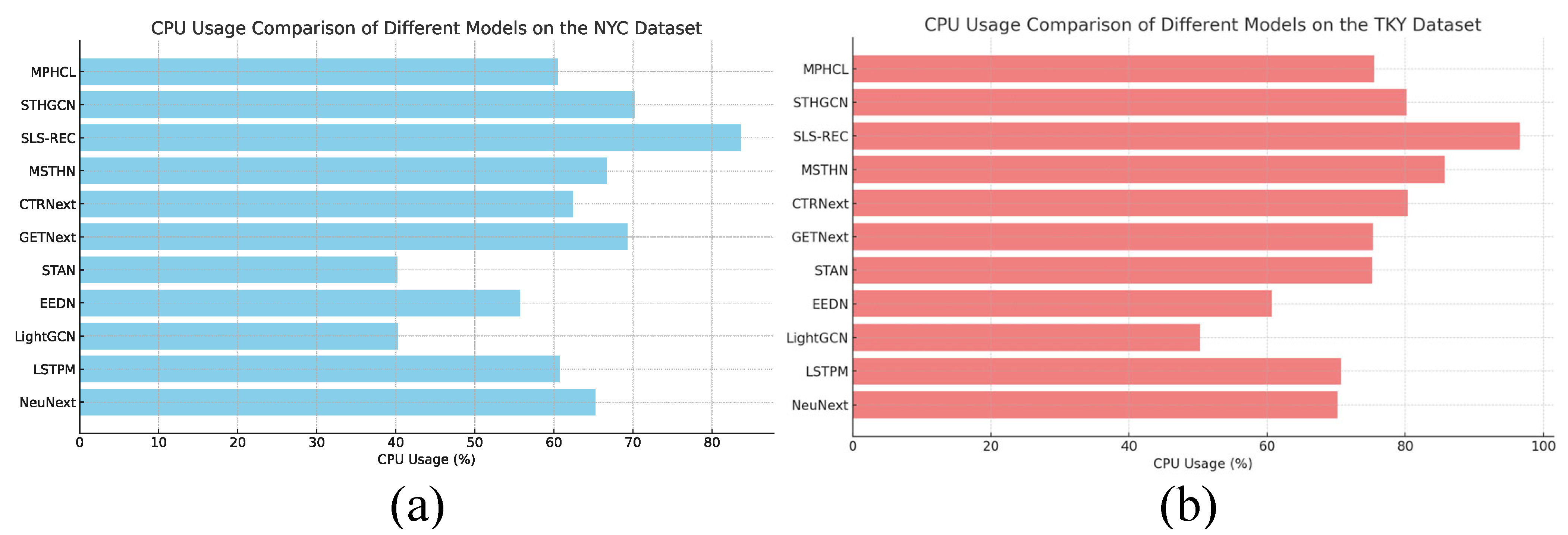
Figure 8 shows the CPU usage comparison of different models. Specifically, our proposed MPHCL model demonstrates a relatively low CPU usage of 60% on the NYC dataset and 75% on the TKY dataset. These results indicate that MPHCL not only performs competitively in terms of prediction accuracy but also operates efficiently, making it suitable for real-time applications with mobile users who update their location data frequently.

5.7. Hyperparameter Analysis

We analyze the impact of the temperature hyperparameter $\tau$ and the distance threshold ${\mathrm{\Delta }}_d$ on the model performance, measured by Recall@5, on both the NYC and TKY datasets. The temperature hyperparameter $\tau$ is commonly used in contrastive learning frameworks (e.g., InfoNCE loss), where it controls the concentration level of the similarity distribution. Specifically, a smaller $\tau$ sharpens the distribution, amplifying differences between similar and dissimilar pairs, while a larger $\tau$ smooths it. In our case, we observe that the optimal value is $\tau =0.5$, which balances these effects and leads to the highest recall performance across different distance thresholds.

In Figure 9a, we observe that, when $\tau =0.5$, Recall@5 reaches its peak for all values of ${\mathrm{\Delta }}_d$. Among these, ${\mathrm{\Delta }}_d=2.0 \mathrm{km}$ yields the best performance. This can be attributed to the spatial characteristics of NYC, where location predictions are densely clustered, particularly in Manhattan. Hence, a relatively small distance threshold is sufficient to capture the relevant local geographical context.

In contrast, Figure 9b shows that, while $\tau =0.5$ is still optimal, the best-performing distance threshold is ${\mathrm{\Delta }}_d=2.5 \mathrm{km}$, slightly larger than that of NYC. This is because the location predictions in Tokyo are more geographically dispersed across a wider urban area. As a result, a larger ${\mathrm{\Delta }}_d$ is necessary to incorporate a broader spatial context and effectively capture semantic relationships in the data.

In summary, while the optimal temperature hyperparameter $\tau$ remains consistent across datasets at $\tau =0.5$, the optimal distance threshold ${\mathrm{\Delta }}_d$ varies due to differences in location prediction density and spatial distribution. NYC benefits from a smaller ${\mathrm{\Delta }}_d$ due to its compact urban layout, whereas TKY requires a larger threshold to accommodate its broader geographical spread.

To investigate the sensitivity of our Disentangled Hypergraph Representation Learning Network to architectural configurations, we conduct a comprehensive evaluation over varying embedding dimensions $d\in \{32,64,128,256\}$ and layer numbers $L\in \{1,2,3,4\}$, as shown in Figure 10.

The performance surface formed by varying d and L reveals the following key observations:

(1) On the NYC dataset, the model attains the maximum performance Recall@5 = 0.4350 at $(d=128,L=2)$. This setting, corresponding to an intermediate embedding size and a two-layer network, strikes an effective balance between representation capacity and overfitting risk.

(2) On the TKY dataset, the optimal setting shifts slightly to a deeper architecture, Recall@5 = 0.3630 at $(d=128,L=3)$. Despite the difference in optimal depth, both datasets consistently favor an embedding dimension of $d=128$, suggesting this size as a robust choice across domains.

(3) We observe a non-monotonic relationship between both d and L with performance. When the embedding size is too small (e.g., $d=32$), the model suffers from insufficient representational capacity, leading to degraded performance due to its inability to capture complex hyper-relational patterns. As d increases, performance improves, peaking at $d=128$, after which further increases (e.g., $d=256$) lead to a decline. This degradation for larger d is attributed to feature redundancy, which not only increases the computational cost but may also introduce noise, harming generalization. A similar pattern is observed with respect to network depth L. Shallow networks ($L=1$) tend to under-express structural dependencies, while overly deep networks ($L=4$) suffer from over-smoothing or optimization difficulties. The optimal number of layers thus lies at a moderate depth.

(4) In conclusion, the experimental results empirically demonstrate that a moderate embedding size ($d=128$) coupled with a shallow-to-moderate network depth ($L=2$ or $L=3$) offers the best trade-off between model expressiveness and generalization. This validates the importance of carefully tuning these architectural hyperparameters for achieving optimal performance in disentangled hypergraph representation learning.

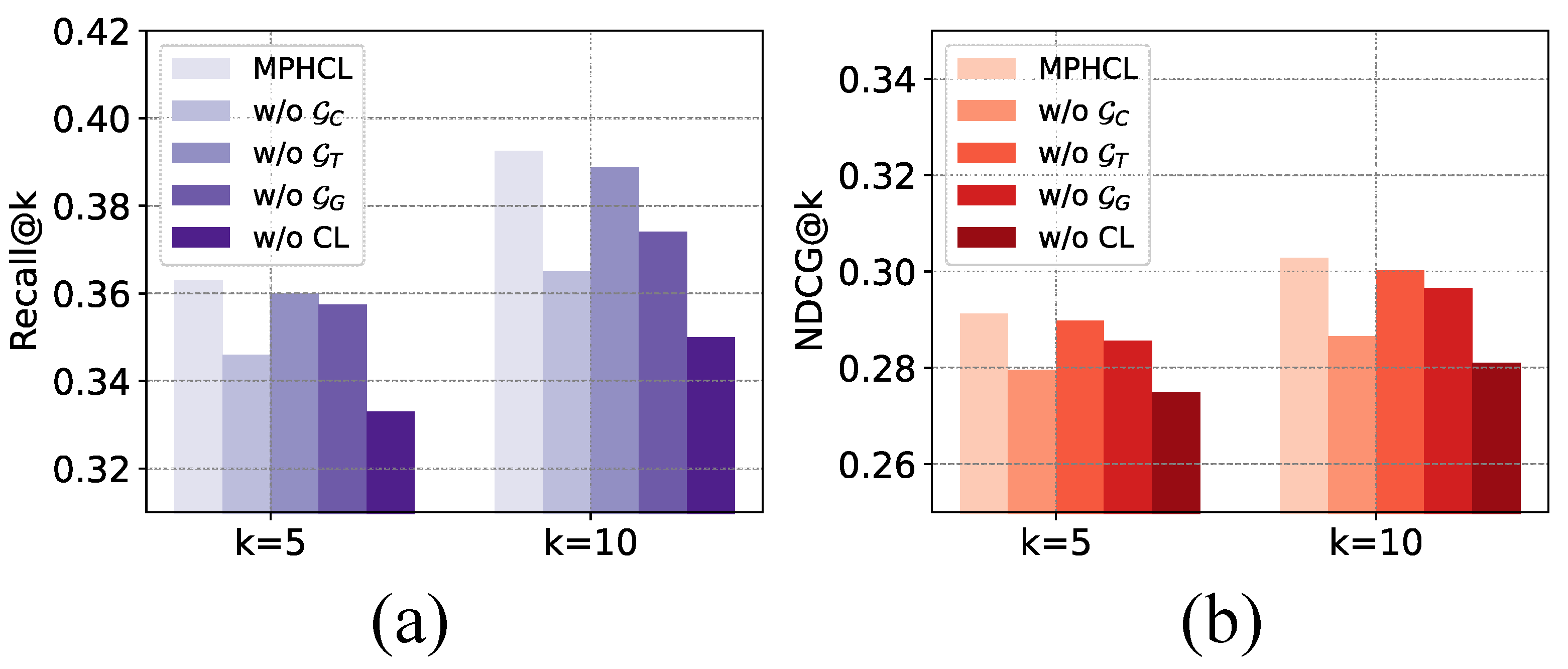
5.8. Ablation Study

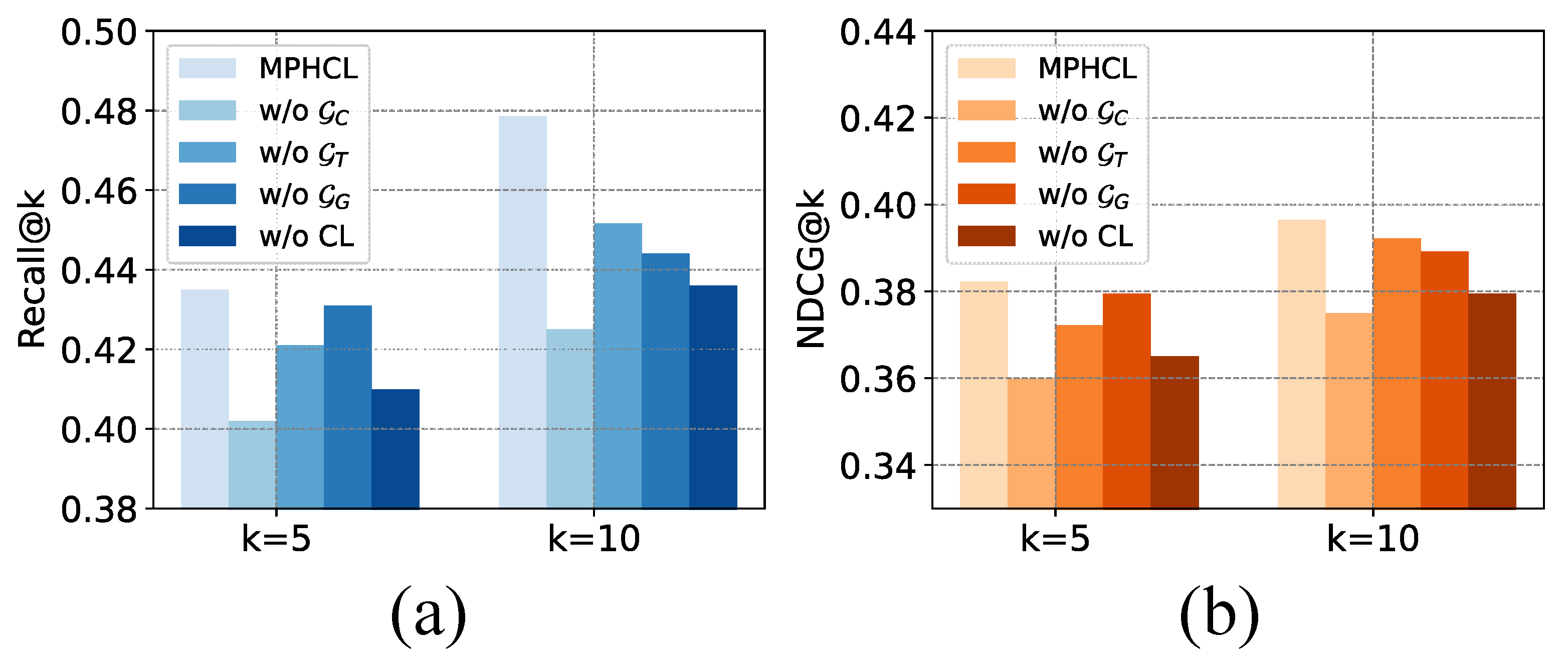
To comprehensively evaluate the effectiveness of each individual module within our proposed MPHCL framework, we conduct a detailed ablation study on two representative datasets—NYC and TKY—as illustrated in Figure 11 and Figure 12. The full MPHCL model is denoted as the baseline, while “w/o X” indicates the model variant without component X. For each variant, we compare the performance using Recall@K and NDCG@K metrics.

• w/o ${\mathcal{G}}_C$ represents removing the collective preference hypergraph.
• w/o ${\mathcal{G}}_T$ represents removing the global transition flow graph.
• w/o ${\mathcal{G}}_G$ represents removing the geospatial context hypergraph.
• w/o CL represents removing cross-view contrastive learning from the full MPHCL model.

The key four findings are summarized as follows:

• On the NYC dataset, the removal of the collective preference hypergraph (${\mathcal{G}}_C$) leads to the most pronounced decline in both Recall@K and NDCG@K scores. This indicates that capturing collaborative signals among users and items through high-order relations plays a central role in recommendation accuracy within dense urban environments like NYC, where user behaviors tend to be highly co-dependent. The contrastive learning module is the second most impactful, demonstrating that enforcing representational consistency and discrimination among hypergraph views significantly improves generalization. By contrast, the geospatial context hypergraph (${\mathcal{G}}_G$) and global transition flow graph (${\mathcal{G}}_T$) contribute to more modest gains. Notably, the global transition flow graph shows the least degradation when removed, implying that short-term behavioral transitions play a relatively minor role in this context, possibly due to the less sequentially structured urban mobility patterns of NYC users.
• In the TKY dataset, the contrastive learning module emerges as the most crucial component, with its absence resulting in the most substantial drop in both performance metrics. This can be attributed to the relatively sparse and more heterogeneous nature of user behaviors in Tokyo, where enforcing consistency across hypergraph-structured views becomes essential for learning robust representations. The collective preference hypergraph follows as the second most important component, reflecting the residual importance of collaborative user-item interactions. Interestingly, in contrast to NYC, the geospatial context hypergraph contributes more than the global transition flow graph, highlighting the stronger influence of location-based preferences in TKY’s wider spatial layout. These results suggest that different urban characteristics and user interaction patterns lead to varying dependencies on spatial, sequential, and collaborative cues.
• Across both datasets, a consistent pattern emerges in how the ranking cutoff K affects the relative importance of modules. At $K=5$, where top-ranked predictions are emphasized, the global transition flow graph tends to be more influential than the geospatial context hypergraph, especially in the NYC dataset. This suggests that recent user behaviors and transition dynamics play a larger role in fine-grained recommendation scenarios. However, as K increases to 10, the Geospatial Context Hypergraph becomes more impactful. This shift can be explained by the fact that geographic cues, though more stable and less temporally sensitive, contribute to broader diversity in larger recommendation lists, while the directed nature of sequential transitions is more localized and immediate in its influence.
• Finally, despite dataset-specific differences, several general conclusions can be drawn. For NYC, the collective preference hypergraph dominates in importance, aligning with the city’s denser and more homogeneous behavioral patterns, where user co-preferences are strong and informative. For TKY, the contrastive learning component proves to be the most essential, underscoring its role in overcoming data sparsity and enhancing the expressiveness of learned embeddings. Additionally, the geospatial context hypergraph shows greater relative importance in TKY due to the city’s broader geographic dispersion, where modeling spatial proximity is vital for meaningful recommendations. In both cases, the full MPHCL model consistently outperforms all its ablated counterparts, thereby validating the synergistic effect of jointly modeling collaborative, global transition flow, and spatial patterns under a contrastive learning framework.

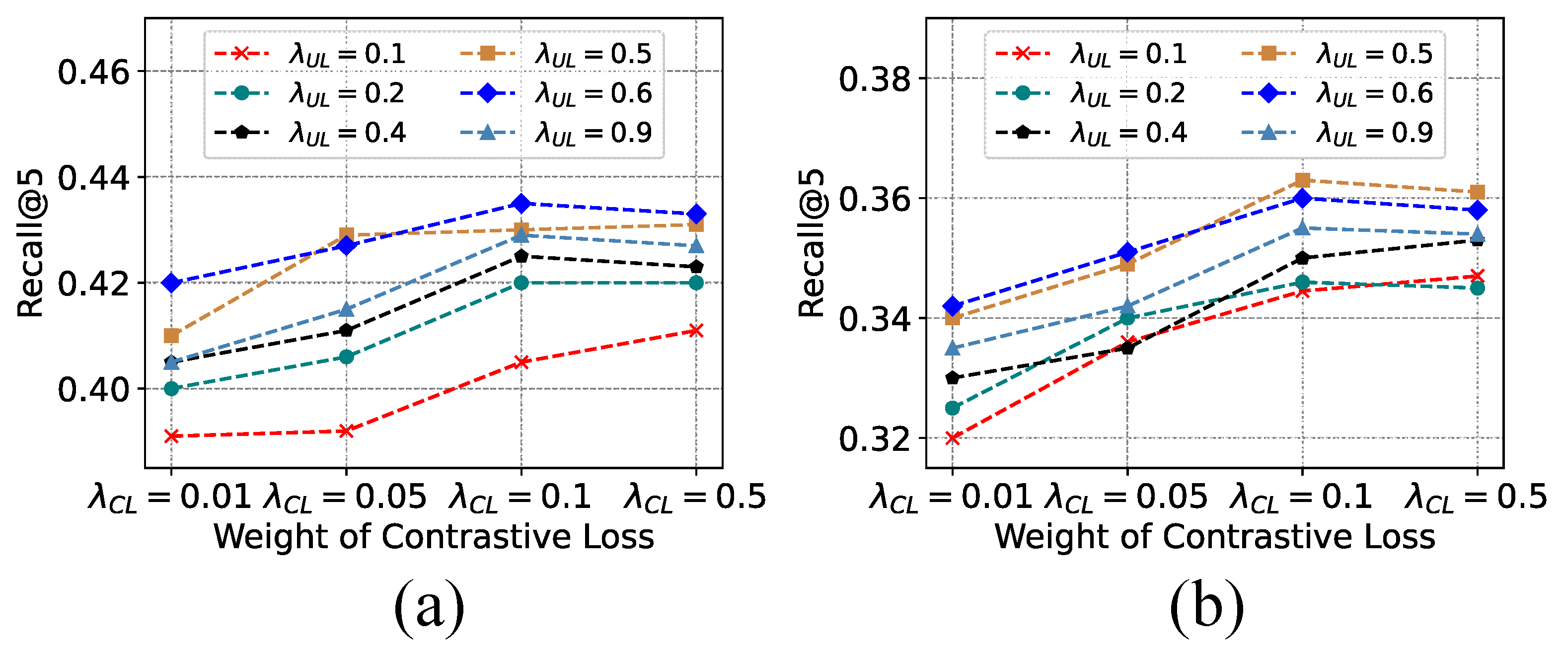
5.9. In-Depth Study

To further explore the influence of contrastive learning on model performance, we conduct a deep investigation into the effect of varying the contrastive loss weight. As shown in Figure 13, we compare different configurations of contrastive loss (${\lambda }_{CL}$) and the fusion coefficient (${\lambda }_{UL}$) for user and location views, across two datasets: (a) NYC and (b) TKY. The Recall@5 scores under different parameter settings reveal key insights into how these components contribute to the overall recommendation performance.

From the results, it is evident that contrastive learning significantly enhances the model’s ability to capture useful representations, particularly in the NYC dataset. As ${\lambda }_{CL}$ increases, Recall@5 consistently improves across most ${\lambda }_{UL}$ settings, confirming the importance of contrastive objectives in aligning representations under different contexts. This trend persists, albeit less prominently, in the TKY dataset, suggesting contrastive learning also plays a beneficial role in sparser or differently distributed spatial environments.

In addition to the contrastive loss weight, the fusion weight ${\lambda }_{UL}$—which balances the contributions of the user view and the location view—also shows a noticeable effect. For the NYC dataset, the best performance is achieved when ${\lambda }_{UL}=0.6$, indicating that the user-centric view is slightly more influential than the location-centric view. In contrast, the TKY dataset achieves optimal performance around ${\lambda }_{UL}=0.5$, suggesting both views contribute equally and should be treated with the same level of importance.

These findings suggest that, in denser urban environments like NYC, where users frequently interact with a diverse set of locations, the personalization aspect (user view) is more critical. Conversely, in less dense or differently structured environments like Tokyo, user preferences and location characteristics are more balanced in importance. This nuanced understanding supports the necessity of adaptively weighting contrastive signals based on regional characteristics and data density.

To further validate the effectiveness of our geospatial modeling, Figure 14 and Figure 15 visualize the learned geographical view hypergraph ${\mathcal{G}}_G$ on the NYC and TKY dataset. The left panel overlays the correlation of different locations on an actual city map, revealing highly dense and complex spatial dependence. The right panel presents a structural abstraction of the hypergraph, illustrating the connectivity among locations and the spatial relationships captured by our MPHCL model. The hypergraph constructed for the NYC dataset contains 3835 nodes and 2160 edges, with an average degree of 0.5632. This relatively low average degree, despite the large number of nodes, highlights the sparsity and diversity of user interactions across the spatial landscape. Such complexity underscores the need for robust context modeling, which our contrastive framework effectively captures.

5.10. Discussion

Our approach could also support transport network design by providing accurate predictions of user mobility patterns, which can be leveraged to optimize the placement of transport hubs, designing dynamic routing systems, and improving the efficiency of public transport services. By accurately forecasting user preferences for specific locations, our model can help in designing systems that are more aligned with actual user behavior, thus enhancing the overall efficiency of transportation networks.

In travel demand modeling and next-location prediction, it is common to face challenges due to insufficient or sparse data. To address this, big data, particularly floating car data (FCD), has emerged as a valuable resource for calibrating model parameters. FCD provides comprehensive vehicle movement data, which helps to more accurately estimate travel demand and predict users’ future movements by capturing traffic patterns across both spatial and temporal dimensions. The FCD data might serve as an external, complementary source of information that helps refine predictions when user trajectory data is sparse or noisy. To further enhance the model’s performance in scenarios with limited information, we plan to incorporate FCD in future work. By using real-time vehicle trajectory data, FCD can aid in calibrating user behavior patterns. This data can help us capture flow patterns in geographically diverse areas, improving the accuracy of user visits to the next location, especially in data-sparse or noisy environments.

6. Conclusions

In this study, we proposed MPHCL, a novel multi-perspective learning framework designed to address the inherent limitations of existing location prediction models, which often conflate heterogeneous behavioral signals into entangled latent spaces. By constructing dedicated hypergraphs that reflect collaborative preferences, global transition flow dynamics, and geospatial contexts, respectively, MPHCL captures high-order relationships that traditional graph-based and sequence models overlook. The proposed disentangled hypergraph representation learning network employs a two-step propagation scheme—within-hyperedge and across-hyperedge aggregation—to effectively isolate and refine the semantic contribution of each behavioral factor. Moreover, we integrate a cross-view contrastive learning module that encourages alignment between view-specific embeddings, thus enhancing the coherence, robustness, and generalizability of learned representations. Comprehensive experiments on two datasets confirm that MPHCL consistently achieves superior performance across all evaluation metrics compared to a broad range of strong baselines, including RNN-based, GCN-based, and hypergraph-based models. The average recall improvement ranges from 7.05% to 7.81%, the average NDCG improvement ranges from 5.77% to 12.60%, and the average MRR improvement ranges from 4.21% to 10.45%. Ablation studies further demonstrate the individual effectiveness of each module, while sensitivity analyses highlight the importance of hyperparameter selection for spatial and representational granularity.