PSCDR-BMPNet: A Point-Supervised Contrastive Deep Regression Network for Point Cloud Biomass Prediction

Abstract

Accurate assessment of above-ground biomass (AGB) is essential for optimizing crop growth and enhancing agricultural efficiency. However, predicting above-ground biomass (AGB) presents significant challenges. Traditional point cloud networks often struggle with processing crop structures and data characteristics, hindering their ability to predict biomass accurately. To address these limitations, we propose a point-supervised contrastive deep regression method (PSCDR) and a novel network, BMP_Net (BioMixerPoint_Net). The PSCDR method leverages the benefits of deep contrastive regression while accounting for the modal differences between point cloud and 2D image data. By incorporating Chamfer distance to measure point cloud similarity, it improves the model’s adaptability to point cloud features. Experimental results on the SGCBP public dataset show that PSCDR significantly reduces prediction errors compared to seven other point cloud models. Furthermore, the BMP_Net network, which integrates the novel PFMixer module and a point cloud downsampling module, effectively captures the relationship between point cloud structure, density, and biomass. The model achieved test results with RMSE, MAE, and MAPE values of 75.92, 63.19, and 0.115, respectively, outperforming PointMixer by 37.94, 30.07, and 0.079. This method provides an efficient biomass monitoring tool for precision agriculture.

1. Introduction

Above-ground biomass (AGB) is a critical indicator for evaluating crop growth status. It not only reflects the health and productive potential of crops but also correlates closely with final crop yield [1,2,3]. Accurate prediction of above-ground biomass provides valuable information for growers and researchers, enabling the optimization of crop management strategies. By scientifically adjusting the application rates of fertilizers, pesticides, and irrigation water, it is possible to enhance both the yield and quality of agricultural products [4].

Moreover, predicting above-ground biomass is crucial for adjusting the operational parameters of harvesting machinery. This biomass directly influences the intake rate of harvesting equipment, and inappropriate intake levels can adversely affect the efficiency and performance of these machines [5,6].

Traditional methods for monitoring above-ground biomass face numerous limitations and drawbacks, often involving destructive processes [7,8]. With advancements in computing and the increasing maturity of deep learning algorithms, such as deep regression networks (DRNs) [9], non-destructive methods for predicting above-ground biomass have been increasingly adopted. Compared to conventional monitoring techniques, deep learning-based approaches offer significant advantages [10,11].

In deep learning, regression tasks typically encompass several research areas, including deep imbalanced regression, ordinal regression, general continuous-value regression, and contrastive regression. These areas are not mutually exclusive, as overlaps exist between different research directions. Yang investigated the issue of data imbalance in deep learning regression tasks, defining deep imbalanced regression (DIR) [12]. Wang proposed a probabilistic deep learning model called Variational Imbalanced Regression (VIR) [13], designed to handle imbalanced regression problems while naturally providing uncertainty estimation.

Shi introduced a novel rank-consistent ordinal regression method, CORN, which addresses the limitations of weight-sharing constraints in existing approaches [14]. Wang studied CRGA [15], a method that leverages contrastive learning for unsupervised gaze estimation generalization in the target domain. Zha proposed Rank-N-Contrast (RNC) [16], which incorporates contrastive learning to rank contrastive samples in the target space, ensuring that learned representations align with the target order. Keramati introduced ConR [17], a contrastive regularization method for addressing imbalanced regression problems in deep learning. By simulating global and local label similarities in the feature space, ConR effectively tackles the challenges of imbalanced regression. The Momentum Contrast (MoCo) method by He et al. introduced a momentum encoder for updating encoder parameters [18]. Additionally, methods like Deep Infomax (DIM) and Contrastive Predictive Coding (CPC) have played pivotal roles in advancing self-supervised learning [19,20].

With the rapid development of 3D acquisition technologies, 3D sensors have become increasingly widespread. These sensors capture rich geometric, shape, and scale information. Three-dimensional data can be represented in various formats, such as depth images, point clouds, and meshes, with point clouds being the preferred format in many scenarios [21]. Methods that use LiDAR (Light Detection and Ranging) sensors to acquire point cloud data have found extensive applications in agriculture and forestry [22,23,24].

For instance, Revenga utilized drones equipped with LiDAR sensors to monitor two agricultural fields in Denmark, collecting point cloud data. They employed an extremely randomized trees regressor to predict biomass [25]. Song developed a tree-level biomass estimation model based on LiDAR point cloud data, extracting features, such as tree height and trunk diameter, and using a Gaussian process regressor to associate these features with tree biomass [26]. Colaco assessed spatial variability in crop biomass in a 64-hectare wheat field using LiDAR technology [27]. Similarly, Ma extracted 56 features using LiDAR technology to estimate forest above-ground biomass (AGB) and its components. They ranked and optimized these features using variable importance projection values derived from partial least squares regression [28].

Seely compared direct and additive models for estimating tree biomass components using point cloud data, employing dynamic graph convolutional neural networks and octree convolutional networks [29]. Pan proposed BioNet, a point cloud processing network for wheat biomass prediction, which incorporated attention-based fusion blocks for final biomass predictions [30]. Oehmcke developed a deep learning system to predict tree volume, AGB, and above-ground carbon stocks directly from LiDAR point cloud data, showing that an improved Minkowski convolutional neural network achieved the best regression performance [31]. Lei introduced BioPM, an end-to-end prediction network that leveraged the upward growth characteristics of crops in wheat fields. Experimental results on public datasets demonstrated that BioPM outperformed both state-of-the-art non-deep learning methods and other deep learning approaches [32]. Oehmcke et al. proposed a point cloud regression method based on Minkowski convolutional neural networks, which significantly improved the accuracy of forest biomass prediction [33].

However, the existing methods for processing point cloud data often rely on basic geometric features, overlooking higher-order structures and multi-scale characteristics. This leads to a feature space that struggles to accurately reflect the mapping relationship between biomass and point cloud structures. Furthermore, biomass data inherently exhibits imbalance, and current deep learning methods have yet to effectively address the issue of features from minority samples being overlooked.

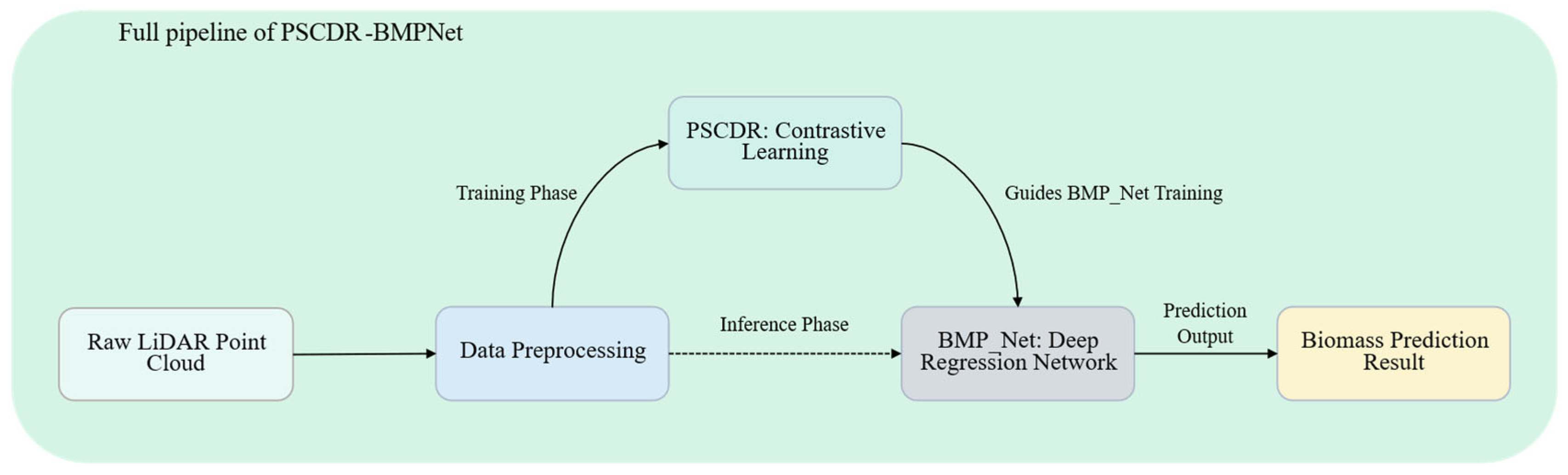
To address the aforementioned challenges, this study proposed a point cloud-based deep contrastive regression method, Point Supervised Contrastive Deep Regression (PSCDR), which leverages the Chamfer distance metric to measure similarity between point clouds, fully utilizing their geometric properties. Additionally, a deep regression network, BMP_Net (BioMixerPoint_Net), incorporating neighbor point attention, was developed to enhance the capability of processing crop structural information. The objective is to provide a reference for rapid and accurate estimation of above-ground biomass and to enable dynamic monitoring.

2. Materials and Methods

2.1. Dataset

The dataset used in this study was the publicly available SGCBP (Small Grain Cereals Biomass Prediction) dataset [30], with data sourced from field experiments conducted in 2019 at Yanco, New South Wales, Australia. The experiment involved sowing 26 varieties of small grain cereals (wheat and barley) at two different densities—250 seeds per square meter and 50 seeds per square meter—resulting in a total of 156 plots. Each plot was scanned at two distinct growth stages: the early stage (August, vegetative phase) and the late growth stage (October, flowering phase). A LiDAR system was employed at a height of 2 m to generate point cloud data during the scans. Following the LiDAR scanning, ground samples were collected from each plot. In the early stage, samples were collected from a 1-square-meter area, while in the flowering stage, samples were collected from a 0.5-square-meter area. The samples were dried at 70 °C for 7 days until a constant weight was achieved, after which the above-ground biomass (AGB) per unit area (g/m²) was calculated. The dataset comprised 306 point clouds along with their corresponding manually measured ground-truth AGB data. The dataset was split into 204 training plots and 102 testing plots. A visualization of the SGCBP point cloud data is presented in Figure 1, displaying, from left to right, the top view, side view, and oblique view, respectively.

2.2. PSCDR: A Deep Contrastive Regression Method for Point Cloud Data

The PSCDR method is inspired by InfoNCE [20] and ConR [17], and it is better suited to the requirements of deep regression tasks, effectively enhancing the performance of deep regression tasks, including above-ground biomass prediction. PSCDR generates positive sample pairs and augmented samples for anchor selection by applying rotation and scaling transformations to the point cloud data of the same agricultural field. In supervised contrastive learning, PSCDR computes the loss by integrating both sample features and label similarity, ensuring that samples with similar biomass values are positioned closer in the feature space, while samples with larger differences are positioned farther apart.

2.2.1. Problem Definition

The point cloud biomass prediction task can be defined as follows: Given a point cloud set $\mathrm{S}\in {\mathrm{P}}^{\mathrm{D}}$, $\mathrm{S}=\left\{{\mathrm{P}}_{\mathrm{i}}\left|\mathrm{i}=\mathrm{1,2},\dots ,\mathrm{n}\right.\right\}$, containing $\mathrm{n}$ unordered points, where each point ${\mathrm{P}}_{\mathrm{i}}$ is represented as a vector $({\mathrm{x}}_{\mathrm{i}},{\mathrm{y}}_{\mathrm{i}},{\mathrm{z}}_{\mathrm{i}})$ in three-dimensional space, and ${\mathrm{P}}_{\mathrm{i}}\in {\mathrm{P}}^{\mathsf{\Delta }}$. Now, given a set containing $\mathrm{N}$ point cloud sets $\mathrm{S}$ and their corresponding labels $\mathrm{l}$, the set is denoted as ${\left\{\left({\mathrm{S}}_{\mathrm{i}},{\mathrm{l}}_{\mathrm{i}}\right)\right\}}_{\mathrm{i}=0}^{\mathrm{N}}$, where ${\mathrm{l}}_{\mathrm{i}}\in {\mathrm{P}}^{{\mathrm{D}}^{\prime }}$. Here, a feature encoder $\mathsf{\Pi }\left(\cdot \right)$ was designed to encode the point cloud set $\mathrm{S}$, along with a regression prediction function $\mathrm{P}\left(\cdot \right)$. These two components together formed the regression prediction model, where the predicted label ${\widehat{\mathrm{l}}}_{\mathrm{i}}=\mathrm{P}\left(\mathsf{\Pi }\left({\mathrm{S}}_{\mathrm{i}}\right)\right)$. The objective was to minimize the L1-distance between the model’s predicted values and the true labels ${\mathrm{l}}_{\mathrm{i}}$.

2.2.2. Anchor Data and Pair Selection

For a given point cloud sample set ${\left\{\left({\mathrm{S}}_{\mathrm{i}},{\mathrm{l}}_{\mathrm{i}}\right)\right\}}_{\mathrm{i}=0}^{\mathrm{N}}$, the augmented sample set is ${\left\{\left({\tilde{\mathrm{S}}}_{\mathrm{j}},{\tilde{\mathrm{l}}}_{\mathrm{j}}\right)\right\}}_{\mathrm{j}=0}^{2\mathrm{N}}$, where ${\tilde{\mathrm{S}}}_{2\mathrm{k}-1}={\mathrm{e}}^{\prime }\left({\mathrm{S}}_{\mathrm{k}}\right)$ and ${\tilde{\mathrm{S}}}_{2\mathrm{k}}=\mathrm{e}\left({\mathrm{S}}_{\mathrm{k}}\right)$, with $\mathrm{e}(\cdot )$ and ${\mathrm{e}}^{\prime }(\cdot )$ being independent point cloud augmentation operations. For each point cloud set ${\mathrm{S}}_{\mathrm{k}}$, after two independent augmentations, ${\tilde{\mathrm{S}}}_{2\mathrm{k}}$ and ${\tilde{\mathrm{S}}}_{2\mathrm{k}-1}$ are derived from ${\mathrm{S}}_{\mathrm{k}}$, where $\mathrm{k}\in \left[0,\mathrm{N}\right]$. The corresponding labels for the augmented point cloud sets remain unchanged, meaning ${\tilde{\mathrm{l}}}_{2\mathrm{k}}={\tilde{\mathrm{l}}}_{2\mathrm{k}-1}={\mathrm{l}}_{\mathrm{k}}$.

The two augmented samples, $\left({\tilde{\mathrm{S}}}_{\mathrm{i}},{\tilde{\mathrm{l}}}_{\mathrm{i}}\right)$ and $\left({\tilde{\mathrm{S}}}_{\mathrm{j}},{\tilde{\mathrm{l}}}_{\mathrm{j}}\right)$, are passed through the feature encoder $\mathsf{\Pi }\left(\cdot \right)$ to generate two feature vectors ${\mathrm{f}}_{\mathrm{i}}=\mathsf{\Pi }\left({\tilde{\mathrm{S}}}_{\mathrm{i}}\right)$ and ${\mathrm{f}}_{\mathrm{j}}=\mathsf{\Pi }\left({\tilde{\mathrm{S}}}_{\mathrm{j}}\right)$. These are then processed by the regression function $\mathrm{P}\left(\cdot \right)$ to obtain ${\widehat{\mathrm{l}}}_{\mathrm{i}}$ and ${\widehat{\mathrm{l}}}_{\mathrm{j}}$. For the selection of positive and negative sample pairs, a similarity function is used to calculate whether the similarity between the two label values or predicted values exceeds a threshold.

The anchor point data selection still follows the anchor point data selection method. For each sample j, $\left({\tilde{\mathrm{S}}}_{\mathrm{j}},{\tilde{\mathrm{l}}}_{\mathrm{j}}\right)$, the feature vector sets of its positive and negative sample pairs are represented as ${\mathrm{E}}_{\mathrm{j}}^{+}=\{({\mathrm{f}}_{\mathrm{p}}){\}}_{\mathrm{p}=0}^{{\mathrm{N}}_{\mathrm{j}}^{+}}$ and ${\mathrm{E}}_{\mathrm{j}}^{-}=\{({\mathrm{f}}_{\mathrm{q}}){\}}_{\mathrm{q}=0}^{{\mathrm{N}}_{\mathrm{j}}^{-}}$, where ${\mathrm{N}}_{\mathrm{j}}^{+}$ is the number of positive samples and ${\mathrm{N}}_{\mathrm{j}}^{-}$ is the number of negative samples. If ${\mathrm{N}}_{\mathrm{j}}^{-}>0$, the sample $\left({\tilde{\mathrm{S}}}_{\mathrm{j}},{\tilde{\mathrm{l}}}_{\mathrm{j}}\right)$ was considered an anchor point. The sample pairing process of the PSCDR algorithm is illustrated in Figure 2.

2.2.3. Supervised Contrastive Loss for Point Cloud and Deep Regression

The PSCDR method is designed to handle point cloud data and introduces the loss function ${\mathsf{\Lambda }}_{\mathrm{P}\mathrm{S}\mathrm{C}\mathrm{D}{\mathrm{R}}_{\mathrm{j}}}$. For sample j, if it is not selected as an anchor point data, then ${\mathsf{\Lambda }}_{\mathrm{P}\mathrm{S}\mathrm{C}\mathrm{D}{\mathrm{R}}_{\mathrm{j}}}=0$. Otherwise, the loss function minimizes the distance between positive sample point cloud pairs in the feature space while proportionally increasing the distance between negative sample point cloud pairs based on the similarity of their labels and feature values. In simpler terms, this loss function aims to pull features of positive point cloud pairs (those with similar biomass labels and originating from the same augmented sample) closer together in the feature space while pushing features of negative pairs (those with dissimilar labels or features) further apart. The degree of repulsion for negative pairs is scaled by their label and feature dissimilarity. The specific formula is as follows:

$${\mathsf{\Lambda }}_{\mathrm{P}\mathrm{S}\mathrm{C}\mathrm{D}{\mathrm{R}}_{\mathrm{j}}}=-\log {\displaystyle \frac{1}{{\mathrm{N}}_{\mathrm{j}}^{+}}}\sum _{{\mathrm{f}}_{\mathrm{i}}\in {\mathrm{E}}_{\mathrm{j}}^{+}}{\displaystyle \frac{\exp ({\mathrm{f}}_{\mathrm{j}}\cdot {\mathrm{f}}_{\mathrm{i}}/\mathsf{\tau })}{{\sum }_{{\mathrm{f}}_{\mathrm{p}}\in {\mathrm{E}}_{\mathrm{j}}^{+}}\exp ({\mathrm{f}}_{\mathrm{j}}\cdot {\mathrm{f}}_{\mathrm{p}}/\mathsf{\tau })+{\sum }_{{\mathrm{f}}_{\mathrm{q}}\in {\mathrm{E}}_{\mathrm{j}}^{-}}{\mathrm{T}}_{\mathrm{j},\mathrm{q}}\exp ({\mathrm{f}}_{\mathrm{j}}\cdot {\mathrm{f}}_{\mathrm{q}}/\mathsf{\tau })}}$$

(1)

where $\mathsf{\tau }$ is the temperature parameter and ${\mathrm{f}}_{\mathrm{j}}$ is the feature vector produced by the feature encoder for the anchor point data. ${\mathrm{T}}_{\mathrm{j},\mathrm{q}}$ represents the repulsion between each point cloud negative sample pair, and its calculation formula is as follows:

$${\mathrm{T}}_{\mathrm{j},\mathrm{q}}={\mathrm{p}}_{\mathrm{s}}\left(\mathsf{\theta },\mathrm{S}\mathrm{i}{\mathrm{m}}_{\mathrm{l}}\left({\tilde{\mathrm{l}}}_{\mathrm{j}},{\tilde{\mathrm{l}}}_{\mathrm{q}}\right),\mathrm{S}\mathrm{i}{\mathrm{m}}_{\mathrm{p}\mathrm{f}}\left({\mathrm{f}}_{\mathrm{j}},{\mathrm{f}}_{\mathrm{q}},{\tilde{\mathrm{S}}}_{\mathrm{j}},{\tilde{\mathrm{S}}}_{\mathrm{q}}\right)\right)$$

(2)

In Equation (2), ${\mathrm{p}}_{\mathrm{s}}(·)$ is the repulsion calculation function for negative sample pairs, ${\tilde{\mathrm{l}}}_{\mathrm{q}}$ represents the label value of the augmented sample ${\tilde{\mathrm{S}}}_{\mathrm{q}}$, $\mathsf{\theta }$ is the weight coefficient, and $\mathrm{S}\mathrm{i}{\mathrm{m}}_{\mathrm{l}}\left(\cdot ,\cdot \right)$ and $\mathrm{S}\mathrm{i}{\mathrm{m}}_{\mathrm{p}\mathrm{f}}\left(\cdot ,\cdot ,\cdot ,\cdot \right)$ are the label similarity calculation function and the sample feature similarity calculation function, respectively. The calculated value of ${\mathrm{T}}_{\mathrm{j},\mathrm{q}}$ is directly proportional to $\mathsf{\theta }$ and $\mathrm{S}\mathrm{i}{\mathrm{m}}_{ \mathrm{ppf}}\left({\mathrm{f}}_{\mathrm{j}},{\mathrm{f}}_{\mathrm{q}},{\tilde{\mathrm{S}}}_{\mathrm{j}},{\tilde{\mathrm{S}}}_{\mathrm{q}}\right)$ and inversely proportional to $\mathrm{S}\mathrm{i}{\mathrm{m}}_{\mathrm{l}}\left({\tilde{\mathrm{l}}}_{\mathrm{j}},{\tilde{\mathrm{l}}}_{\mathrm{q}}\right)$. For the $\mathrm{S}\mathrm{i}{\mathrm{m}}_{\mathrm{p}\mathrm{f}}$ similarity calculation function, both the similarity between feature vectors and the similarity between the original point cloud data are taken into account. Point cloud data differs significantly from 2D image data in modality and carries rich structural and spatial information. Therefore, considering only the similarity between feature vectors (f) generated by the encoder might lead to the loss of some original spatial information. To address this, the Chamfer distance metric is introduced to calculate the similarity between point cloud negative sample pairs, while cosine similarity is used to calculate the similarity between feature vectors. This formula combines two aspects of similarity: the first term, involving cosine similarity, measures how aligned the feature vectors ${\mathrm{f}}_{\mathrm{j}}$ and ${\mathrm{f}}_{\mathrm{q}}$ are (higher cosine similarity means more aligned). The second term, ${\mathrm{d}}_{\mathrm{C}\mathrm{D}}$, measures the geometric dissimilarity between the original point clouds ${\tilde{\mathrm{S}}}_{\mathrm{j}}$ and ${\tilde{\mathrm{S}}}_{\mathrm{q}}$ using Chamfer distance (lower Chamfer distance means more similar shapes). The coefficients $\mathsf{\mu }$ and $\mathsf{\lambda }$ balance the contribution of these two similarity aspects. The calculation formula for $\mathrm{S}\mathrm{i}{\mathrm{m}}_{\mathrm{p}\mathrm{f}}$ is as follows:

$$\mathrm{S}\mathrm{i}{\mathrm{m}}_{\mathrm{p}\mathrm{f}}\left({\mathrm{f}}_{\mathrm{j}},{\mathrm{f}}_{\mathrm{q}},{\tilde{\mathrm{S}}}_{\mathrm{j}},{\tilde{\mathrm{S}}}_{\mathrm{q}}\right)=\mathsf{\mu }\cdot {\displaystyle \frac{1}{\mathrm{C}\mathrm{o}\mathrm{s}\mathrm{s}\mathrm{i}\mathrm{m}({\mathrm{f}}_{\mathrm{j}},{\mathrm{f}}_{\mathrm{q}})+2}}+\mathsf{\lambda }\cdot {\mathrm{d}}_{\mathrm{C}\mathrm{D}}({\tilde{\mathrm{S}}}_{\mathrm{j}},{\tilde{\mathrm{S}}}_{\mathrm{q}})$$

(3)

$${\mathrm{d}}_{\mathrm{C}\mathrm{D}}({\tilde{\mathrm{S}}}_{\mathrm{j}},{\tilde{\mathrm{S}}}_{\mathrm{q}})={\displaystyle \frac{1}{\left|{\tilde{\mathrm{S}}}_{\mathrm{j}}\right|}}{\sum }_{{\mathrm{p}}_{\mathrm{x}}\in {\tilde{\mathrm{S}}}_{\mathrm{j}}}\underset{{\mathrm{p}}_{\mathrm{y}}\in {\tilde{\mathrm{S}}}_{\mathrm{q}}}{\mathrm{m}\mathrm{i}\mathrm{n}}{‖{\mathrm{p}}_{\mathrm{x}}-{\mathrm{p}}_{\mathrm{y}}‖}_2^2+{\displaystyle \frac{1}{\left|{\tilde{\mathrm{S}}}_{\mathrm{q}}\right|}}{\sum }_{{\mathrm{p}}_{\mathrm{y}}\in {\tilde{\mathrm{S}}}_{\mathrm{q}}}\underset{{\mathrm{p}}_{\mathrm{x}}\in {\tilde{\mathrm{S}}}_{\mathrm{j}}}{\mathrm{m}\mathrm{i}\mathrm{n}}{‖{\mathrm{p}}_{\mathrm{y}}-{\mathrm{p}}_{\mathrm{x}}‖}_2^2$$

(4)

where $\mathrm{C}\mathrm{o}\mathrm{s}\mathrm{s}\mathrm{i}\mathrm{m}(\cdot ,\cdot )$ is the cosine similarity calculation function and ${\mathrm{d}}_{\mathrm{C}\mathrm{D}}(\cdot ,\cdot )$ is the function used to compute the Chamfer distance value. For two point cloud samples, a larger Chamfer distance indicates greater dissimilarity between the two sets of point clouds. According to Equation (3), the more similar the two point cloud samples, the smaller the sum of the first and second components; conversely, the less similar the two samples, the larger the sum of the first and second components. ${\tilde{\mathrm{S}}}_{\mathrm{j}}$ and ${\tilde{\mathrm{S}}}_{\mathrm{q}}$ are two sets of augmented point clouds, and $\left|{\tilde{\mathrm{S}}}_{\mathrm{j}}\right|$ and $\left|{\tilde{\mathrm{S}}}_{\mathrm{q}}\right|$ represent the number of points contained in each set. In Equation (4), the first term represents the average of the sum of the minimum distances from any point ${\mathrm{p}}_{\mathrm{x}}$ in ${\tilde{\mathrm{S}}}_{\mathrm{j}}$ to ${\tilde{\mathrm{S}}}_{\mathrm{q}}$, while the second term represents the average of the sum of the minimum distances from any point ${\mathrm{p}}_{\mathrm{y}}$ in ${\tilde{\mathrm{S}}}_{\mathrm{q}}$ to ${\tilde{\mathrm{S}}}_{\mathrm{j}}$.

The loss function ${\mathsf{\Lambda }}_{\mathrm{P}\mathrm{S}\mathrm{C}\mathrm{D}\mathrm{R}}$ is defined as the average value of the sum of the losses for all augmented samples, expressed as:

$${\mathsf{\Lambda }}_{\mathrm{P}\mathrm{S}\mathrm{C}\mathrm{D}\mathrm{R}}={\displaystyle \frac{1}{2\mathrm{N}}}{\sum }_{\mathrm{j}=0}^{2\mathrm{N}}{\mathsf{\Lambda }}_{\mathrm{P}\mathrm{S}\mathrm{C}\mathrm{D}{\mathrm{R}}_{\mathrm{j}}}$$

(5)

The total loss function is the weighted sum of the ${\mathsf{\Lambda }}_{\mathrm{P}\mathrm{S}\mathrm{C}\mathrm{D}\mathrm{R}}$ and the regression loss, expressed as:

$${\mathsf{\Lambda }}_{\mathrm{s}\mathrm{u}\mathrm{m}}^{\mathrm{P}\mathrm{S}\mathrm{C}\mathrm{D}\mathrm{R}}={\mathsf{\alpha }}_2{\mathsf{\Lambda }}_{\mathrm{P}}+{\mathsf{\beta }}_2{\mathsf{\Lambda }}_{\mathrm{P}\mathrm{S}\mathrm{C}\mathrm{D}\mathrm{R}}$$

(6)

2.3. BMP_Net: A Point Cloud Deep Regression Network Incorporating Neighbor Attention

2.3.1. Construction of the PFMixer Module

When using LiDAR to scan point cloud data for crop biomass prediction tasks, the scan results typically encompass various crop components, including above-ground fruits, stems, and leaves. However, in the field environment where crops grow, various types of debris and ground point clouds often exist as interfering factors. As a result, the scanned data inevitably contain a significant amount of noise.

To enhance point cloud processing efficiency and the ability to extract relevant point cloud data, this study proposes the PFMixer module, which employs two point cloud processing methods: intra-set mixing and inter-set mixing. These methods aim to accurately identify target point clouds and establish relationships between the target point clouds and biomass during training and learning. By integrating the PFMixer module into the deep learning model, it becomes possible to better extract meaningful point cloud information from a mixture of redundant and useful data, thereby improving the model’s accuracy in identifying target point clouds.

As illustrated in Figure 3, a point set p and its corresponding features x are input into the PFMixer module. After neighbor selection through the kNN module, the data proceeds to the intra-set mixing module. This module performs interaction computations within each point set, updating the features of neighboring point sets, followed by processing through a ReLU activation function. The features then enter the inter-set mixing module, where point features are propagated across different point cloud data, again processed by a ReLU activation function, and subjected to an SOP (Symmetric Operation Pooling) operation. Throughout this process, three cross-level residual shortcut branches are introduced to integrate the original point cloud information with the processed point cloud data, aiming to more comprehensively establish the relationship between the point cloud and biomass.

2.3.2. Construction of the Point Cloud Transition Downsampling Module

Point cloud networks, similar to convolutional neural networks, require downsampling operations to reduce the density of the data transmitted through the network. The Point Cloud Transition Downsampling module proposed in this paper is designed to decrease the density of point cloud data, thereby reducing computational complexity and memory consumption, while improving the model’s efficiency. This module helps in extracting important features, reducing noise and redundant information, enhancing the model’s generalization ability, and mitigating the risk of overfitting.

The overall structure of the PTransDown (Point Transition Down Block) module is shown in Figure 4. It includes hierarchical set mixing, farthest point sampling, neighborhood query and grouping, channel contraction, Softmax normalization, and linear layers. Through farthest point sampling, the module selects representative points from the original point cloud to preserve key information. Next, feature information undergoes hierarchical set mixing and neighborhood query and grouping, enabling feature interaction and local feature acquisition. The channel contraction module reduces the dimensionality of neighborhood features, decreasing computational complexity. Softmax normalization determines feature weights, providing a reference for feature integration. The linear transformation module maps the input features to the output space and extracts feature information. Finally, the linear layer outputs the feature, which is fused with the hierarchical set mixing output features, offering decision support for the biomass prediction task. These steps work collaboratively, allowing the PTransDown module to effectively reduce the dimensionality of point cloud data, extract key features, and provide a foundation for biomass prediction tasks.

2.3.3. N2P Attention: Neighborhood Point Attention Network

N2P Attention is a key attention mechanism specifically designed for point cloud data processing [34]. Its structure includes three main components: query (Q), key (K), and value (V), and it works by calculating the correlation between a point and its neighbors to capture local information. Since point cloud data typically has complex structures and high-dimensional features, traditional methods struggle to effectively capture local information and relationships. N2P Attention, on the other hand, can capture the information from the neighbors surrounding each point, allowing for a better understanding of the local structures and features within point cloud data. This results in improved accuracy and performance in biomass prediction tasks. By introducing N2P Attention, the network can more fully leverage the relationships between the points in the cloud, enabling the model to make more accurate predictions of biomass while maintaining efficiency and flexibility when processing large-scale and complex point cloud data. The structure of N2P Attention is illustrated in Figure 5.

2.3.4. Construction of the Overall BMP_Net Structure

The network benefits from the PointMixer [35] framework structure, utilizing multiple cross-layer residual connections to facilitate information exchange. This design effectively explores the relationship between point cloud structure, point cloud density, and the corresponding biomass. The architecture of BMP_Net is shown in Figure 6. Initially, the point cloud data is converted into low-dimensional vectors through an Embedding layer, enabling the neural network to learn and process the data effectively. The N2P Attention module then processes the Embedding output and point information, capturing crucial details about the neighbors of each point, thus enhancing the point cloud data processing performance. The data is further processed by the PFMixer module, point cloud transition downsampling module, and N2P Attention, followed by a BatchNorm normalization layer. These modules are combined in three consecutive stages, deepening the extraction of point cloud features while compressing the feature data, which facilitates efficient point cloud network computation.

Finally, the network passes through a global pooling layer, followed by a Smooth MLP (Multi-Layer Perceptron) to output the predicted biomass value. In summary, BMP_Net integrates key components that improve information extraction efficiency when processing point cloud data, enhancing the accuracy and performance of biomass prediction tasks.

2.4. Overall PSCDR-BMPNet Pipeline Summary

Having detailed the SGCBP dataset (Section 2.1), the proposed Point Supervised Contrastive Deep Regression (PSCDR) method (Section 2.2) and the architecture of the BioMixerPoint Network (BMP_Net), including its constituent modules (Section 2.3), Figure 7 provides a holistic view of the entire PSCDR-BMPNet pipeline for point cloud biomass prediction.

As illustrated, the process initiates with Raw LiDAR Point Cloud data. This data first undergoes Data Preprocessing, which includes steps such as point cloud sampling and any necessary cleaning or normalization.

During the Training Phase, the preprocessed data is utilized by both the PSCDR: Contrastive Learning module and the BMP_Net: deep regression network. The PSCDR module (Section 2.2) generates augmented data views and computes a contrastive loss that encourages the learning of discriminative features sensitive to biomass variations. This contrastive objective effectively guides the BMP_Net training process, supplementing its primary regression task of predicting biomass. The BMP_Net (Section 2.3) itself processes the point cloud features through its specialized architecture to learn the mapping to biomass.

In the subsequent Inference Phase, only the trained BMP_Net is active. New, preprocessed point cloud data is fed directly into the BMP_Net, which then outputs the Biomass Prediction Result. The PSCDR mechanism contributes to the robustness and accuracy of the BMP_Net through the knowledge embedded in its trained weights during the joint training phase. The following section will present the experimental results validating this approach.

3. Results

3.1. The Experimental Setup and Evaluation Metrics

The experiment was conducted using Ubuntu 20.04.4 LTS 64-bit as the operating system, with an Intel Xeon Silver 4214 processor (Intel Corporation, Santa Clara, CA, USA) running at CPU@2.20 GHz and 32 GB of RAM. The GPUs used were two NVIDIA Tesla T4 (NVIDIA Corporation, Santa Clara, CA, USA), with a total of 32 GB of video memory. The software environment was built based on the Python 3.8.19 programming language, using the PyTorch 1.13.1 deep learning framework with CUDA 11.7 acceleration. Key dependency libraries included OpenCV 4.10.0 and TorchVision 0.14.1 for computer vision processing, Torch-Pruning 1.5.2 for model compression, NumPy 1.24.3 and SciPy 1.10.1 for scientific computing, as well as Pandas 1.5.3 for data manipulation. The GPU acceleration environment was implemented via CUDA Toolkit 11.7 and cuDNN 8.5.0, with versions strictly compatible with the PyTorch framework to ensure computational stability. The Adam optimizer was employed, with 80 training epochs, and cosine annealing decay was used for the learning rate. Other hyperparameters were set according to those published in the SGCBP paper. The performance of the proposed methods and models was evaluated using three metrics: RMSE, MAE, and MAPE (Mean Absolute Percentage Error). RMSE, MAE, and MAPE were chosen as they are standard and comprehensive metrics for evaluating the accuracy of regression models, reflecting different aspects of prediction error.

3.2. Comparative Experiments

In addition to the models from the SGCBP paper, this study also included PointMixer [35], Point Transformer [36], and PointNeXt [37] as comparison models. It is important to note that in the SGCBP paper, the authors did not use the MAPE metric; therefore, the data presented in

Table 1. Performance of different models on the SGCBP dataset (data for PointNet to BioNet is from paper [30], where the original paper’s authors did not use the MAPE metric).

Models\Metrics	RMSE	MAE	MAPE
PointNet [30]	189.80	139.61	None
PointNet++ [30]	188.85	142.80	None
DGCNN [30]	161.61	129.66	None
GS-Net [30]	180.85	145.63	None
3DVI [30]	151.79	115.15	None
BioNet [30]	99.33	71.23	None
PointMixer	113.41	93.26	0.194
Point Transformer	155.49	128.74	0.230
PointNeXt	146.96	116.76	0.215
BMP_Net	84.48	67.31	0.131

from the SGCBP paper do not include MAPE values. PointMamba [38] was not included in the comparison because it focuses on classification rather than regression. While classical machine learning regressors (e.g., Random Forest, Support Vector Regression with hand-crafted features) represent an alternative approach, the scope of this study was to benchmark against contemporary deep learning methods specifically designed for or adapted to point cloud data, which have generally demonstrated superior performance in capturing complex 3D spatial patterns for tasks like biomass estimation in the recent literature [9,10,11,29,30,31,32,33]. Future comparative studies could incorporate such classical baselines for a broader perspective.

As shown in Table 1, except for BMP_Net and BioNet, the PointMixer network performs the best among all the unimproved networks. Its RMSE, MAE, and MAPE were 113.41, 93.26, and 0.194, respectively. PointMixer excels in the biomass prediction task using point cloud data, primarily because of its universal and efficient structure, as well as its parameter efficiency and hierarchical response propagation advantages. Its versatility makes it suitable for various types of point cloud data, and the channel-mixing MLP effectively promotes feature aggregation. Additionally, its concise and efficient design improves the efficiency of processing large-scale data. The use of a symmetric encoder–decoder block with a hierarchical response propagation mechanism helps capture complex relationships within the point cloud data, thereby enhancing prediction performance. This result also validated our design choices for BMP_Net, which adapted and improved upon concepts from the PointMixer [35] architecture.

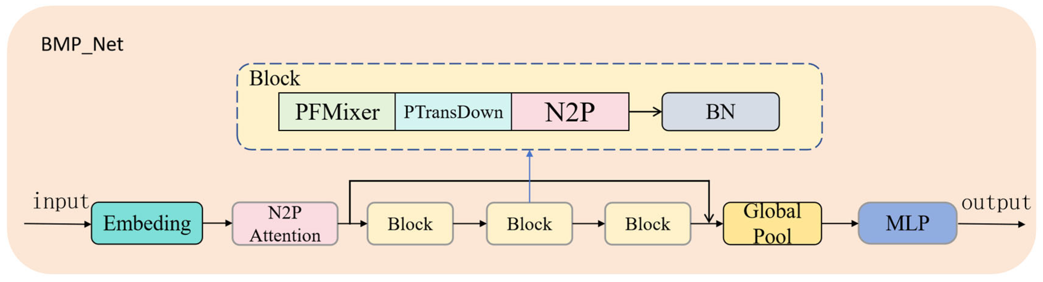
The BMP_Net model proposed in this paper outperforms the BioNet model introduced in the SGCBP paper, showing better performance in RMSE, MAE, and MAPE, with values of 84.8, 67.31, and 0.131, respectively. BMP_Net effectively extracts and utilizes the relevant information from point cloud data by leveraging key components such as the Embedding layer, N2P Attention, PFMixer module, and point cloud downsampling. This significantly improves the accuracy and performance of biomass prediction tasks. The Embedding layer transforms high-dimensional point cloud data into a more manageable vector form, N2P Attention captures local features, the PFMixer module performs deep feature extraction and data compression, and point cloud downsampling reduces noise and redundant information. These components work together to provide a more robust decision-making foundation for biomass prediction tasks.

After applying the PSCDR method, BMP_Net showed a reduction in RMSE, MAE, and MAPE, with decreases of 8.56, 4.12, and 0.016, respectively. This indicates that the PSCDR method plays a significant role in predicting biomass and other regression tasks with point cloud data. The combination of BMP_Net and PSCDR yields the best performance. PSCDR enhances the prediction process by introducing Chamfer distance to calculate the similarity in point cloud data in three-dimensional space while considering the similarity between features. This approach provides strong support for label comparison and label value prediction, contributing to the improved performance of deep regression tasks.

3.3. Effectiveness Analysis of the PSCDR Method

Table 2. Performance of the PSCDR method on different common point cloud models.

Metrics	RMSE		MAE		MAPE
Model\loss	Focal_L1	${\mathsf{\Lambda }}_{\mathrm{sum}}^{\mathrm{PSCDR}}$	Focal_L1	${\mathsf{\Lambda }}_{\mathrm{sum}}^{\mathrm{PSCDR}}$	Focal_L1	${\mathsf{\Lambda }}_{\mathrm{sum}}^{\mathrm{PSCDR}}$
PointNet	192.14	178.30	165.06	137.52	0.312	0.276
PointNet++	187.32	175.42	152.89	130.53	0.284	0.268
DGCNN	157.19	154.41	131.68	127.18	0.235	0.242
PointMixer	113.41	102.11	93.26	77.93	0.194	0.167
PointTransformer	155.49	148.91	128.74	122.87	0.230	0.214
PointNeXt	146.96	134.69	116.76	103.49	0.215	0.198
BMP_Net	84.48	75.92	67.31	63.19	0.131	0.115

shows the performance of common regression loss functions and the proposed PSCDR method on a range of well-known point cloud models, as well as the proposed BMP_Net. In many models, when the loss function is replaced with the proposed total loss function ${\mathsf{\Lambda }}_{\mathrm{s}\mathrm{u}\mathrm{m}}^{\mathrm{P}\mathrm{S}\mathrm{C}\mathrm{D}\mathrm{R}}$, the performance of most models improves on the SGCBP dataset. This result is expected because, in regression tasks, the core objective is to predict target values from input data. Regardless of the data modality, the data is encoded into feature vectors by the encoder in the network. By considering the differences between label values and feature values, and adopting a regression-like approach, it is possible to achieve some level of clustering and relative positioning of positive and negative samples in the feature space.

While PSCDR considers these factors, it also takes advantage of the unique characteristics of point cloud data by using Chamfer distance to measure the similarity between two point cloud samples. The information contained in the feature vectors produced by the encoding process is determined by the model’s point cloud encoder. When using common regression loss functions, both PointMixer and the proposed BMP_Net also perform well.

However, the performance improvement of the PSCDR method on the DGCNN model is not significant. This may be because the DGCNN model utilizes graph convolution operations based on local connections, which primarily focus on capturing local structural information of the point cloud data. This local connectivity approach may limit the model’s ability to capture global features of the point cloud data. Although the PSCDR method considers the similarity between global features, the local connectivity nature of the DGCNN model might not fully leverage the global feature similarity loss in the PSCDR method, thus restricting the performance improvement of PSCDR on this model.

3.4. Ablation Experiments of BMP_Net

3.4.1. Ablation Experiments on the Modules of BMP_Net

To investigate the impact of key structures and modules in BMP_Net on overall performance, a series of ablation experiments was conducted. These experiments involved replacing or removing key modules, and the tests were carried out under identical conditions to validate the importance of each designed module. The results of the ablation study are shown in

Table 3. Ablation experiments on different modules of BMP_Net.

Settings		Case 1	Case 2	Case 3	Case 4	Ours
PFMixer		×	×	✓	✓	✓
Point Cloud Transition Downsampling Module		×	✓	×	✓	✓
N2P Attention		×	✓	✓	×	✓
SGCBP	RMSE	213.47	160.76	172.59	97.67	75.92
	MAE	165.41	137.07	151.04	83.05	63.19
	MAPE	0.301	0.265	0.274	0.142	0.115

. Three design components or modules were ablated, including the PFMixer module, the Point Cloud Transition Downsampling module, and the N2P Attention (Neighbor Point Attention) module. We tested five different scenarios: 1. The model with only the main structure, where the PFMixer module was removed (replaced by the MixerBlock from the PointMixer network), the Point Cloud Transition Downsampling module was substituted by a regular downsampling layer, and the N2P Attention module was excluded. 2. The model with the PFMixer module removed only. 3. The model with the Point Cloud Transition Downsampling module removed only. 4. The model with the N2P Attention module removed only. 5. The full BMP_Net model proposed in this study.

From the table, it can be observed that in Case 1, where all three key modules were removed, the model performance was the worst, which aligns with our expectations. After removing these three critical modules, the model’s ability to extract and process the point cloud structure and features significantly declined. Without the PFMixer module, which performs deep feature extraction and data compression, and given the abundance of redundant information in the data, the model’s performance dropped sharply.

In Case 4, the evaluation metrics outperformed those of Case 2 and Case 3, indicating that the PFMixer module and Point Cloud Transition Downsampling module make significant contributions to the network’s performance. The improvement in performance due to these two modules is not simply a linear addition, suggesting that careful consideration was given to the synergy between the two modules during network design, achieving a result where “one plus one is greater than two.” In both Case 2 and Case 3, where only the PFMixer module or the Point Cloud Transition Downsampling module was removed, the performance dropped significantly compared to Case 5 (the full BMP_Net model). Additionally, Case 4 demonstrated that the N2P Attention module effectively captured the surrounding information of each point, aiding in learning local features and enhancing the overall performance of point cloud data processing. This highlights the importance of N2P Attention in improving the model’s ability to focus on relevant neighborhood information, which contributes to better performance in handling complex point cloud data.

3.4.2. PSCDR Algorithm Parameter Ablation Experiments

To investigate the impact of various parameters on the experimental results, multiple sets of parameter ablation experiments were conducted on the SGCBP dataset.

Table 4. Ablation experiment on the weighting coefficients $\mathsf{\mu }$ and $\mathsf{\lambda }$ or similarity calculation in PSCDR.

$\mathsf{\mu }$	$\mathsf{\lambda }$	RMSE	MAE	MAPE
0.01	0.001	77.48	66.15	0.132
	0.003	82.36	71.69	0.138
	0.005	104.52	86.83	0.170
	0.007	122.49	107.46	0.203
	0.009	188.16	155.32	0.352
0.05	0.001	79.31	65.67	0.119
	0.003	75.92	63.19	0.115
	0.005	81.68	69.38	0.125
	0.007	86.53	73.54	0.149
	0.009	154.63	124.79	0.213
0.1	0.001	99.43	82.45	0.159
	0.003	110.82	90.07	0.164
	0.005	80.55	66.31	0.125
	0.007	82.67	70.76	0.149
	0.009	191.36	152.13	0.292
0.5	0.001	129.39	104.48	0.208
	0.003	91.76	76.12	0.151
	0.005	84.72	71.56	0.143
	0.007	126.83	99.73	0.196
	0.009	100.45	82.21	0.174

presents the ablation experiment results for the weight coefficients used in the similarity computation of Equation (3). In these experiments, four different values of $\mathsf{\mu }$ were selected: 0.01, 0.05, 0.1, and 0.5. The value of $\mathsf{\lambda }$ ranged from 0.001 to 0.009, with a step size of 0.002.

The first weight coefficient $\mathsf{\mu }$ corresponds to the coefficient of the reciprocal of the cosine similarity plus two, while $\mathsf{\lambda }$ represents the weight coefficient for the Chamfer distance between point clouds. Due to the significant variability among negative point cloud samples, the computed Chamfer distance tends to be large and exhibits a wide range of values. Therefore, the range of $\mathsf{\lambda }$ was constrained based on preliminary experiments to ensure the overall value of Equation (3) did not become excessively large, and the optimal values reported in Table 4 were identified through these systematic ablation experiments.

Through multiple experiments, it was observed that under different values of $\mathsf{\mu }$, when $\mathsf{\lambda }$ is greater than or equal to 0.01, all evaluation metrics result in NaN values, indicating that the value of $\mathsf{\lambda }$ should not be too large. As shown in the experimental results in the table, the best performance is achieved when $\mathsf{\mu }=0.05$ and $\mathsf{\lambda }=0.003$. Among the four sets of $\mathsf{\mu }$ values, as $\mathsf{\lambda }$ increases, the overall evaluation metric values increase to varying degrees. This experimental result aligns with the hypothesis: when the value of $\mathsf{\lambda }$ is large, multiplying it with the computed Chamfer distance yields a significantly large value, which, when incorporated into the PSCDR method, may lead to numerical overflow and result in NaN values. Additionally, a larger $\mathsf{\lambda }$ value also contributes to an increase in the evaluation metric values.

To investigate the impact of the temperature coefficient τ on the PSCDR algorithm, temperature coefficient ablation experiments were conducted, with the results summarized in

Table 5. Ablation experiment on the parameter $\mathsf{\tau }$ in PSCDR.

$\mathsf{\tau }$	RMSE	MAE	MAPE
0.03	88.92	72.93	0.159
0.05	132.38	107.49	0.205
0.1	116.12	90.28	0.194
0.2	102.54	81.36	0.162
0.5	75.92	63.19	0.115
0.7	92.66	78.21	0.164
0.9	99.13	80.22	0.167

. As shown in the table, the PSCDR algorithm achieves optimal performance when τ = 0.5. This value was determined through the systematic ablation experiments summarized in Table 5, which explored a range of values to balance model discriminative ability against numerical stability. Compared to image data, point cloud data typically exhibits higher dimensionality and complexity, necessitating a larger temperature parameter to ensure that the contrastive learning algorithm can effectively explore its data space. A larger temperature parameter smooths the overall output of ${\Lambda }_{PSCDR}$, thereby enhancing the model’s performance on point cloud data.

However, for the PSCDR algorithm, both excessively high and excessively low temperature parameters can have detrimental effects. An overly high temperature parameter causes the output distribution of ${\Lambda }_{PSCDR}$ to become excessively smooth, which blurs the differences between samples, diminishes the model’s discriminative ability, and may lead to overfitting. Conversely, the ablation experiments revealed that when $\mathsf{\tau }$ ≤ 0.01, the values of all three evaluation metrics become NaN. This indicates that an excessively low temperature parameter results in an overly sharp output distribution of ${\mathsf{\Lambda }}_{\mathrm{P}\mathrm{S}\mathrm{C}\mathrm{D}\mathrm{R}}$, increasing numerical instability in computations. Such instability may cause numerical overflow or underflow in the loss function, potentially rendering optimization infeasible. Therefore, selecting an appropriate temperature parameter is crucial for the performance of the PSCDR algorithm. While τ = 0.5 was optimal in our experiments on the SGCBP dataset, this parameter generally acts as a hyperparameter that may require tuning (e.g., via a validation set) when applying PSCDR to new datasets or different model architectures, typically by exploring values within a range such as [0.05, 1.0].

3.4.3. Ablation Experiments on the Number of Point Cloud Sampling Points

To determine the optimal number of sampling points for the proposed BMP_Net model, ablation experiments on the number of point cloud sampling points were conducted. The results of these ablation experiments are presented in

Table 6. Ablation experiment on the number of sampled points in point clouds.

num_points	RMSE	MAE	MAPE
1024	89.27	70.48	0.128
2048	87.43	69.72	0.129
4096	75.92	63.19	0.115
8192	81.34	67.91	0.122
16,384	96.17	75.48	0.141

. In the original PCD files, the number of points in the point clouds varies significantly and is often excessively large, making it impractical to directly input all data points into a point cloud network for training. Therefore, the original point cloud data must undergo a sampling process, with the sampled point cloud data serving as the input to the point cloud network. This process is analogous to resizing image data in convolutional neural networks. The FPS (Farthest Point Sampling) algorithm was employed as the sampling method, with the number of sampling points set to powers of 2. According to the experimental results, the performance of the three evaluation metrics reaches its optimum when the number of sampling points is 4096. However, when the number of sampling points is either too small (e.g., num_points = 1024) or too large (e.g., num_points = 16,384), the experimental results exhibit relatively mediocre performance. An insufficient number of sampling points leads to information loss, which prevents the full representation of critical features in the point cloud—such as wheat fruit density information highly correlated with biomass—thereby limiting the model’s ability to learn the relationship between point cloud data and biomass from limited information. Conversely, an excessively large number of sampling points increases the computational burden, resulting in prolonged training times and reduced model inference efficiency. Additionally, excessive point cloud data introduces more redundant information and noise, which may cause the model to overfit the training data, consequently degrading its performance. These ablation studies demonstrate the process of parameter selection and provide insights into model sensitivity, thereby contributing to the justification of our final model configuration.

4. Discussion

The biomass prediction network, BMP_Net, proposed in this study, which is based on point cloud deep contrastive regression, along with the integrated PSCDR (Point Supervised Contrastive Learning for Deep Regression) method, has achieved significant progress in the task of above-ground biomass prediction. This section provides an in-depth discussion of the research findings by integrating prior studies and research hypotheses, focusing on technical contributions, result interpretation, practical applications, limitations, and future research directions, to comprehensively elucidate the scientific significance and potential impact of this study.

4.1. Technical Contributions and Result Interpretation

To address the limitations of traditional point cloud networks in biomass prediction tasks, particularly their insufficient handling of crop structural information and the challenge of uncovering the relationship between point cloud characteristics and biomass, this study proposes the innovative PSCDR method and the BMP_Net network. Revenga et al. [25] employed extremely randomized tree regression, relying solely on statistical features of point cloud height while overlooking the nonlinear impact of crop canopy structure on biomass. Unlike general contrastive learning methods, such as MoCo by He et al. [18] and ConR [17], PSCDR introduces the Chamfer distance metric into the contrastive loss function for the first time, directly quantifying the three-dimensional spatial similarity of point clouds. The incorporation of Chamfer distance significantly enhances the model’s robustness to point cloud deformations. Specifically, PSCDR reduces the RMSE of the PointMixer from 113.41 to 102.11, outperforming ConR [17], which relies solely on label similarity.

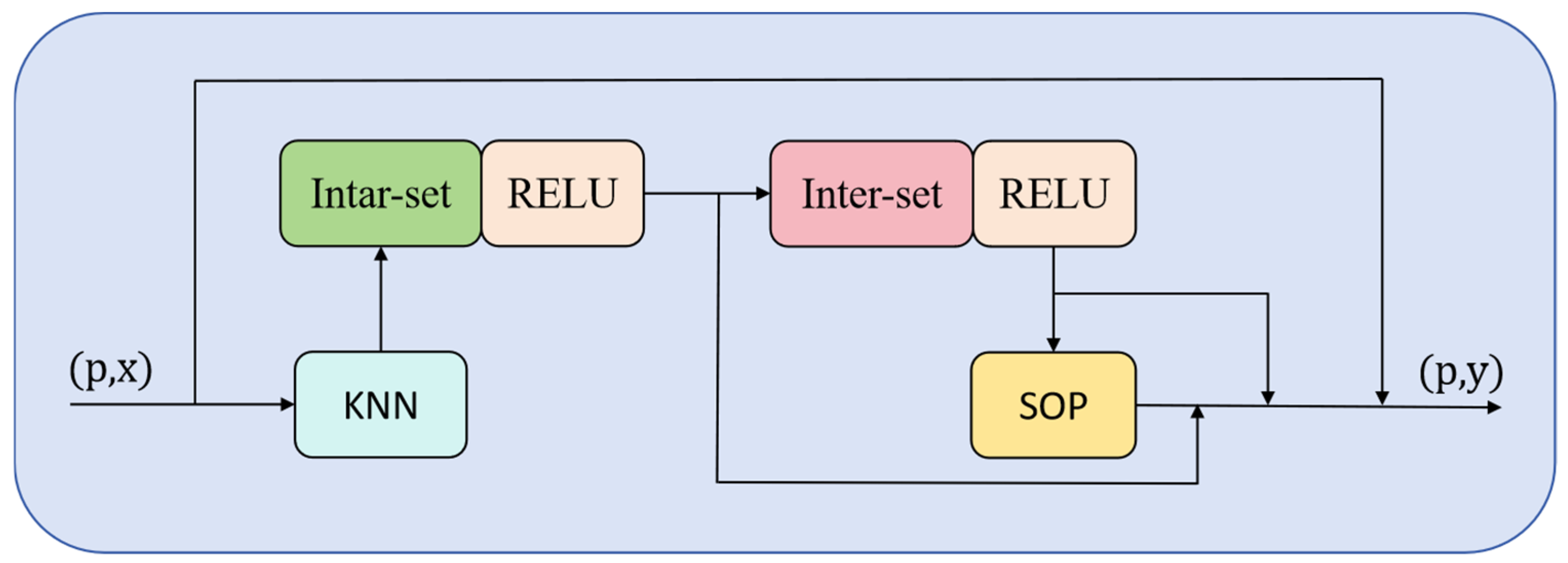
The PFMixer module in BMP_Net enhances local feature interactions through intra-set mixing and captures cross-regional correlations via inter-set mixing. Our ablation studies demonstrate that removing the PFMixer module increases the RMSE from 75.92 to 160.76, underscoring its critical role in noise suppression and feature fusion. This design surpasses the attention fusion block in BioNet [30], which depends solely on global attention, as PFMixer preserves multi-scale information through residual connections.

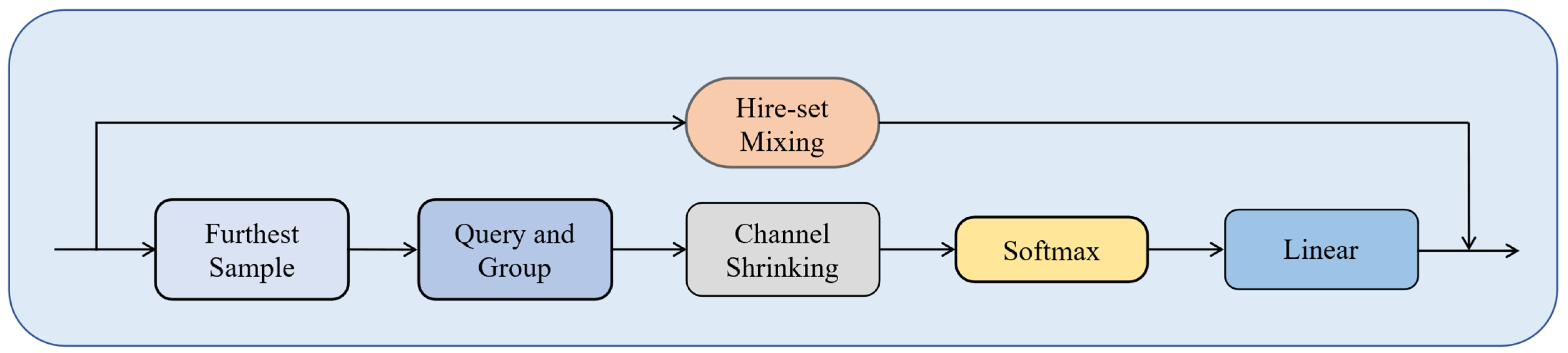
Traditional downsampling methods often lead to the loss of key biomass-related features. For instance, BioNet by Pan et al. [30] suffers from excessive dilution of wheat ear point clouds due to a fixed sampling rate. In contrast, the PTransDown module in BMP_Net prioritizes the retention of dense regions, such as stems and ears, through channel contraction and Softmax normalization. Our ablation experiments reveal that removing this module increases the MAE from 63.19 to 151.04, confirming its importance in preserving critical structural information.

The N2P Attention mechanism enhances sensitivity to fine structures in point clouds by capturing information from the neighbors of each point and applying neighborhood attention weights, enabling the identification of spatial distribution patterns of wheat tillering nodes. With the introduction of N2P Attention, the network more effectively leverages the correlations within point cloud data, allowing for more accurate biomass prediction while maintaining efficiency and flexibility when handling large-scale, complex point cloud datasets.

At the technical level, this study overcomes the modality adaptation bottleneck of point cloud data in regression tasks by developing a high-precision prediction framework through contrastive learning and structured module design. Compared to BioNet by Pan et al. [30], which relies on attention fusion blocks, and BioPM by Lei et al. [32], which focuses on crop growth characteristics, the proposed PSCDR method and BMP_Net architecture achieve deep exploration of point cloud geometric features through modality-adapted contrastive loss and structured module design. This work establishes a methodological foundation for point cloud-based biomass prediction. The reduction in RMSE from 84.48 to 75.92 with the incorporation of PSCDR represents a relative improvement of approximately 10.1%. This level of enhancement in prediction accuracy can be significant in practical agricultural scenarios, for instance, by enabling more precise variable-rate fertilization or more reliable yield estimations.

4.2. Practical Applications

The findings of this study hold significant application value in the field of precision agriculture. Accurate biomass prediction provides data support for crop management, such as optimizing fertilization, irrigation, and pest control strategies, thereby enhancing agricultural production efficiency. Pan et al. [39] proposed NeFF-BioNet, which integrates point clouds and UAV images to predict crop biomass, demonstrating the potential of multimodal approaches. In contrast, the BMP_Net model proposed in this study focuses on LiDAR point clouds, offering an efficient unimodal solution.

Moreover, above-ground biomass is closely related to the feed rate of harvesting machinery [5]. The high-precision predictions of BMP_Net can serve as a basis for adjusting machinery parameters, reducing efficiency losses during equipment operation. On the SGCBP dataset, the combination of BMP_Net and PSCDR achieves a MAPE of only 0.115, significantly outperforming PointMixer’s MAPE of 0.194. This enables reliable technical support for the dynamic monitoring of small grain cereals such as wheat and barley. Compared to traditional manual sampling methods [7,8], this non-destructive prediction approach offers clear advantages in terms of efficiency and sustainability, laying a foundation for the modernization and intelligent development of agriculture. For instance, on a large-scale wheat farm, high-precision biomass maps generated by PSCDR-BMPNet could guide variable-rate nitrogen application by drones, optimizing fertilizer use efficiency for different growth zones and minimizing environmental runoff. Similarly, in barley cultivation, understanding biomass variability can inform decisions on differential harvesting strategies to maximize yield quality.

The incorporation of the PSCDR method with BMP_Net yielded significant performance gains, as evidenced by the reduction in RMSE from 84.48 to 75.92, MAE from 67.31 to 63.19, and MAPE from 0.131 to 0.115 when compared to BMP_Net alone on the SGCBP dataset. These represent relative improvements of approximately 10.13% in RMSE, 6.12% in MAE, and 12.21% in MAPE. Such enhancements in prediction accuracy are of considerable practical importance in precision agriculture. For instance, a reduction of 8.56 g/m² in RMSE translates to a more precise estimation of available plant material per unit area. This increased accuracy can directly inform more efficient N-fertilizer management strategies, potentially leading to optimized fertilizer application rates, reduced input costs, and minimized environmental leaching. Furthermore, more accurate biomass predictions throughout the growing season can contribute to more reliable yield forecasting, aiding farmers and stakeholders in better logistical planning and market engagement. While the definition of “sufficient” accuracy can be application-dependent, these quantitative improvements demonstrate a meaningful step towards more robust and actionable biomass monitoring tools.

4.3. Limitations Analysis and Future Research Directions

Despite the significant progress achieved in this study, several limitations remain:

Limited Dataset Coverage and Applicability: A primary limitation of the current study is its reliance on the SGCBP dataset. Consequently, the presented PSCDR-BMPNet method was specifically validated for the agricultural crops included in this dataset, namely, wheat and barley, and within the geographical and environmental context of New South Wales, Australia, where the data was collected. While the proposed methodological innovations in contrastive learning and network architecture are designed to be generalizable, the direct applicability and performance of the trained model on other crop types (e.g., maize, rice, soybean) or in different agro-ecological regions require further dedicated validation and potential fine-tuning. Future research efforts should prioritize expanding the evaluation to more diverse datasets to ascertain the broader applicability and robustness of the PSCDR-BMPNet.

Computational Efficiency Challenges: BMP_Net exhibits high computational complexity when processing large-scale point cloud data, making it challenging to deploy on edge devices such as drones or field robots.

Need for Improved Multimodal Data Fusion and Noise Robustness: The model relies solely on LiDAR point cloud data and does not incorporate multimodal information such as RGB images, soil moisture, or meteorological data. Additionally, its ability to filter point cloud noise in extreme environmental conditions (e.g., rain, fog, or varying lighting) is limited.

Based on the above analysis, future research can explore the following directions:

Dataset Expansion and Diversity: Expanding the dataset scale to include a broader range of crop types (e.g., maize, rice) and diverse ecological conditions would enhance the model’s robustness and generalization ability.

Model Optimization and Lightweight Design: Bornand et al. [40] utilized deep learning to complete sparse point clouds, addressing occlusion issues in forests. In the future, such methods could be integrated to further enhance the robustness of BMP_Net in complex environments. Optimizing the network architecture to reduce computational costs or employing knowledge distillation to transfer BMP_Net’s knowledge to a lightweight framework could maintain accuracy while lowering computational complexity.

Multisource Data Fusion: Integrating multispectral and thermal infrared remote sensing data could improve the model’s perception of crop physiological states, further enhancing prediction accuracy.

4.4. Model Interpretability Considerations

Understanding how the PSCDR-BMPNet model arrives at its biomass predictions is crucial for building user trust and facilitating practical adoption in precision agriculture. While the current study primarily focused on predictive accuracy, future iterations should incorporate model interpretability techniques. For instance, methods like SHAP (SHapley Additive exPlanations) or LIME (Local Interpretable Model-agnostic Explanations) could be adapted to identify which points or learned features contribute most significantly to the biomass estimates. Given the use of the N2P Attention module, visualizing attention weights could also offer insights into the spatial regions of the point cloud that the model deems most important. Such analyses would not only demystify the “black box” nature of the deep learning model but also potentially guide further model refinement or data acquisition strategies.

5. Conclusions

This paper focused on the task of biomass prediction using point cloud data. Compared to image data, point cloud data offers more comprehensive and detailed spatial information and structural features. To better extract the spatial feature information from point cloud data, we propose a contrastive learning-based method called PSCDR, which introduces Chamfer distance as a new feature metric. Additionally, we propose a deep regression network, BMP_Net, for point cloud biomass prediction tasks. BMP_Net integrates the PFMixer module and Point Cloud Transition Downsampling module, utilizing multiple cross-level residual connections for information exchange to fully explore the relationship between point cloud structure, point cloud density, and the corresponding biomass. On this foundation, the N2P Attention mechanism is introduced to capture and fuse the neighboring point information within the point cloud.

Experiments on the SGCBP public dataset showed that BMP_Net alone achieved RMSE, MAE, and MAPE values of 84.48, 67.31, and 0.131, respectively, outperforming BioNet. After incorporating the PSCDR method, these three key performance metrics are optimized to RMSE = 75.92, MAE = 63.19, and MAPE = 0.115, demonstrating that the method significantly improves prediction accuracy. Furthermore, in experiments with different point cloud networks, adding the PSCDR method leads to performance improvements across all cases, further validating the general applicability and effectiveness of the PSCDR approach. The improved BMP_Net model achieves high recognition accuracy, making it suitable for precise above-ground biomass detection, thus providing strong technical support for research in related fields.

However, this study has certain limitations. The dataset used lacks sufficient diversity in crop types, geographic regions, and growing conditions, which could help enhance the model’s generalization capabilities. Additionally, there is room for improvement in the model’s robustness in complex environments and its computational efficiency. Future research will focus on optimizing the model structure and algorithms, expanding the dataset’s size and diversity, exploring more effective feature extraction and fusion strategies, and strengthening research on model interpretability. These efforts aim to promote the broader application of point cloud data in biomass prediction, providing more accurate and reliable technical support for precision agriculture and ecosystem research. While the improved BMP_Net model achieves high recognition accuracy on the SGCBP dataset, making it suitable for precise biomass detection of wheat and barley under similar conditions, its broader applicability to other crops and regions remains a key area for future investigation.

References

1. Guo, Y.; He, J.; Zhang, H.; Shi, Z.; Wei, P.; Jing, Y.; Yang, X.; Zhang, Y.; Wang, L.; Zheng, G. Improvement of Winter Wheat Aboveground Biomass Estimation Using Digital Surface Model Information Extracted from Unmanned-Aerial-Vehicle-Based Multispectral Images. Agriculture 2024, 14, 378. [Google Scholar] [CrossRef]
2. Yang, Z.; Yu, Z.; Wang, X.; Yan, W.; Sun, S.; Feng, M.; Sun, J.; Su, P.; Sun, X.; Wang, Z.; et al. Estimation of Millet Aboveground Biomass Utilizing Multi-Source UAV Image Feature Fusion. Agronomy 2024, 14, 701. [Google Scholar] [CrossRef]
3. Shen, S.C.; Zhang, J.X.; Chen, M.H.; Li, Z.W.; Sun, S.N.; Yan, X.B. Estimation of Aboveground Biomass and Chlorophyll Content in Different Varieties of Alfalfa Based on UAV Multispectral Data. Spectrosc. Spectr. Anal. 2023, 43, 3847–3852. [Google Scholar]
4. Liu, Y.; Feng, H.; Fan, Y.; Yue, J.; Chen, R.; Ma, Y.; Bian, M.; Yang, G. Improving Potato Above Ground Biomass Estimation Combining Hyperspectral Data and Harmonic Decomposition Techniques. Comput. Electron. Agric. 2024, 218, 108699. [Google Scholar] [CrossRef]
5. Wang, F.; Wang, J.; Ji, Y.; Zhao, B.; Liu, Y.; Jiang, H.; Mao, W. Research on the Measurement Method of Feeding Rate in Silage Harvester Based on Components Power Data. Agriculture 2023, 13, 391. [Google Scholar] [CrossRef]
6. Yang, Z.K.; Fu, L.L.; Tang, C.; Wang, F.M.; Ni, X.D.; Chen, D. Classification Method of Wheat Harvester Feeding Density Based on MobileViT Model. Trans. Chin. Soc. Agric. Mach. 2023, 54 (Suppl. S1), 172–180. [Google Scholar]
7. Singh, B.; Kumar, S.; Elangovan, A.; Vasht, D.; Arya, S.; Duc, N.T.; Swami, P.; Pawar, G.S.; Raju, D.; Krishna, H.; et al. Phenomics Based Prediction of Plant Biomass and Leaf Area in Wheat Using Machine Learning Approaches. Front. Plant Sci. 2023, 14, 1214801. [Google Scholar] [CrossRef]
8. Elangovan, A.; Duc, N.T.; Raju, D.; Kumar, S.; Singh, B.; Vishwakarma, C.; Krishnan, S.G.; Ellur, R.K.; Dalal, M.; Swain, P.; et al. Imaging Sensor-Based High-Throughput Measurement of Biomass Using Machine Learning Models in Rice. Agriculture 2023, 13, 852. [Google Scholar] [CrossRef]
9. Lathuilière, S.; Mesejo, P.; Alameda-Pineda, X.; Horaud, R. A Comprehensive Analysis of Deep Regression. IEEE Trans. Pattern Anal. Mach. Intell. 2019, 42, 2065–2081. [Google Scholar] [CrossRef]
10. Zhang, J.; Zhou, C.; Zhang, G.; Yang, Z.; Pang, Z.; Luo, Y. A Novel Framework for Forest Above-Ground Biomass Inversion Using Multi-Source Remote Sensing and Deep Learning. Forests 2024, 15, 456. [Google Scholar] [CrossRef]
11. Vahidi, M.; Shafian, S.; Thomas, S.; Maguire, R. Pasture Biomass Estimation Using Ultra-High-Resolution RGB UAVs Images and Deep Learning. Remote Sens. 2023, 15, 5714. [Google Scholar] [CrossRef]
12. Yang, Y.Z.; Zha, K.W.; Chen, Y.C.; Wang, H.; Katabi, D. Delving into Deep Imbalanced Regression. In Proceedings of the 38th International Conference on Machine Learning, Vienna, Austria, 8–24 July 2021; pp. 11842–11851. [Google Scholar]
13. Wang, Z.; Wang, H. Variational Imbalanced Regression: Fair Uncertainty Quantification via Probabilistic Smoothing. In Proceedings of the 37th Conference on Neural Information Processing Systems, New Orleans, LA, USA, 10–16 December 2023; pp. 30429–30452. [Google Scholar]
14. Shi, X.; Cao, W.; Raschka, S. Deep Neural Networks for Rank-Consistent Ordinal Regression Based on Conditional Probabilities. Pattern Anal. Appl. 2023, 26, 941–955. [Google Scholar] [CrossRef]
15. Wang, Y.; Jiang, Y.; Li, J.; Ni, B.; Dai, W.; Li, C.; Xiong, H.; Li, T. Contrastive Regression for Domain Adaptation on Gaze Estimation. In Proceedings of the IEEE/CVF Conference on Computer Vision and Pattern Recognition, New Orleans, LA, USA, 19–24 June 2022; pp. 19376–19385. [Google Scholar]
16. Zha, K.; Cao, P.; Son, J.; Yang, Y.; Katabi, D. Rank-N-Contrast: Learning Continuous Representations for Regression. Adv. Neural Inf. Process. Syst. 2024, 36, 17882–17903. [Google Scholar]
17. Keramati, M.; Meng, L.; Evans, R.D. ConR: Contrastive Regularizer for Deep Imbalanced Regression. arXiv 2023, arXiv:2309.06651. [Google Scholar]
18. He, K.; Fan, H.; Wu, Y.; Xie, S.; Girshick, R. Momentum Contrast for Unsupervised Visual Representation Learning. In Proceedings of the IEEE/CVF Conference on Computer Vision and Pattern Recognition, Seattle, TX, USA; 2020; pp. 9729–9738. [Google Scholar]
19. Hjelm, R.D.; Fedorov, A.; Lavoie-Marchildon, S.; Grewal, K.; Bachman, P.; Trischler, A.; Bengio, Y. Learning Deep Representations by Mutual Information Estimation and Maximization. arXiv 2018, arXiv:1808.06670. [Google Scholar]
20. Oord, A.; Li, Y.; Vinyals, O. Representation Learning with Contrastive Predictive Coding. arXiv 2018, arXiv:1807.03748. [Google Scholar]
21. Vinodkumar, P.K.; Karabulut, D.; Avots, E.; Ozcinar, C.; Anbarjafari, G. A Survey on Deep Learning Based Segmentation, Detection and Classification for 3D Point Clouds. Entropy 2023, 25, 635. [Google Scholar] [CrossRef]
22. Islam, M.; Bijjahalli, S.; Fahey, T.; Gardi, A.; Sabatini, R.; Lamb, D.W. Destructive and Non-Destructive Measurement Approaches and the Application of AI Models in Precision Agriculture: A Review. Precis. Agric. 2024, 25, 1127–1180. [Google Scholar] [CrossRef]
23. Debnath, S.; Paul, M.; Debnath, T. Applications of LiDAR in Agriculture and Future Research Directions. J. Imaging 2023, 9, 57. [Google Scholar] [CrossRef]
24. Rivera, G.; Porras, R.; Florencia, R.; Sánchez-Solís, J.P. LiDAR Applications in Precision Agriculture for Cultivating Crops: A Review of Recent Advances. Comput. Electron. Agric. 2023, 207, 107737. [Google Scholar] [CrossRef]
25. Revenga, J.C.; Trepekli, K.; Oehmcke, S.; Jensen, R.; Li, L.; Igel, C.; Gieseke, F.C.; Friborg, T. Above-Ground Biomass Prediction for Croplands at a Sub-Meter Resolution Using UAV–LiDAR and Machine Learning Methods. Remote Sens. 2022, 14, 3912. [Google Scholar] [CrossRef]
26. Song, Q.; Albrecht, C.M.; Xiong, Z.; Zhu, X.X. Biomass Estimation and Uncertainty Quantification from Tree Height. IEEE J. Sel. Top. Appl. Earth Obs. Remote Sens. 2023, 16, 4833–4845. [Google Scholar] [CrossRef]
27. Colaco, A.F.; Schaefer, M.; Bramley, R.G.V. Broadacre Mapping of Wheat Biomass Using Ground-Based LiDAR Technology. Remote Sens. 2021, 13, 3218. [Google Scholar] [CrossRef]
28. Ma, J.; Zhang, W.; Ji, Y.; Huang, J.; Huang, G.; Wang, L. Total and Component Forest Aboveground Biomass Inversion via LiDAR-Derived Features and Machine Learning Algorithms. Front. Plant Sci. 2023, 14, 1258521. [Google Scholar] [CrossRef]
29. Seely, H.; Coops, N.C.; White, J.C.; Montwé, D.; Winiwarter, L.; Ragab, A. Modelling Tree Biomass Using Direct and Additive Methods with Point Cloud Deep Learning in a Temperate Mixed Forest. Sci. Remote Sens. 2023, 8, 100110. [Google Scholar] [CrossRef]
30. Pan, L.; Liu, L.; Condon, A.G.; Estavillo, G.M.; Coe, R.A.; Bull, G.; Stone, E.A.; Petersson, L.; Rolland, V. Biomass Prediction with 3D Point Clouds from LiDAR. In Proceedings of the IEEE/CVF Winter Conference on Applications of Computer Vision, Waikoloa, HI, USA, 3–8 January 2022; pp. 1330–1340. [Google Scholar]
31. Oehmcke, S.; Li, L.; Trepekli, K.; Revenga, J.C.; Nord-Larsen, T.; Gieseke, F.; Igel, C. Deep Point Cloud Regression for Above-Ground Forest Biomass Estimation from Airborne LiDAR. Remote Sens. Environ. 2024, 302, 113968. [Google Scholar] [CrossRef]
32. Lei, Y.; Ma, H. BioPM: Mixer for Point Cloud Based Biomass Prediction. In Proceedings of the 41st Chinese Control Conference, Hefei, China, 25–27 July 2022; pp. 6363–6367. [Google Scholar]
33. Oehmcke, S.; Li, L.; Revenga, J.C.; Nord-Larsen, T.; Trepekli, K.; Gieseke, F.; Igel, C. Deep Learning Based 3D Point Cloud Regression for Estimating Forest Biomass. In Proceedings of the 30th International Conference on Advances in Geographic Information Systems, Seattle, WA, USA, 1–4 November 2022; pp. 1–4. [Google Scholar]
34. Wu, C.Z.; Zheng, J.W.; Pfrommer, J.; Beyerer, J. Attention-Based Point Cloud Edge Sampling. In Proceedings of the IEEE/CVF Conference on Computer Vision and Pattern Recognition, Vancouver, BC, Canada, 17–24 June 2023; pp. 5333–5343. [Google Scholar]
35. Choe, J.; Park, C.; Rameau, F. Pointmixer: Mlp-mixer for point cloud understanding. In Proceedings of the 17th European Conference on Computer Vision, Tel Aviv, Israel, 23–27 October 2022; pp. 620–640. [Google Scholar]
36. Zhao, H.S.; Jiang, L.; Jia, J.Y.; Torr, P.H.S.; Koltun, V. Point Transformer. In Proceedings of the IEEE/CVF International Conference on Computer Vision, Montreal, QC, Canada, 11–17 October 2021; pp. 16259–16268. [Google Scholar]
37. Qian, G.; Li, Y.; Peng, H.; Mai, J.; Hammoud, H.; Elhoseiny, M.; Ghanem, B. PointNeXt: Revisiting PointNet++ with Improved Training and Scaling Strategies. Adv. Neural Inf. Process. Syst. 2022, 35, 23192–23204. [Google Scholar]
38. Liang, D.K.; Zhou, X.; Xu, W.; Zhu, X.K.; Zou, Z.K.; Ye, X.Q.; Tan, X.; Bai, X. PointMamba: A Simple State Space Model for Point Cloud Analysis. arXiv 2024, arXiv:2402.10739. [Google Scholar]
39. Li, X.; Hayder, Z.; Zia, A.; Cassidy, C.; Liu, S.; Stiller, W.; Stone, E.; Conaty, W.; Petersson, L.; Rolland, V. NeFF-BioNet: Crop Biomass Prediction from Point Cloud to Drone Imagery. arXiv 2024, arXiv:2410.23901. [Google Scholar]
40. Bornand, A.; Abegg, M.; Morsdorf, F.; Rehush, N. Completing 3D Point Clouds of Individual Trees Using Deep Learning. Methods Ecol. Evol. 2024, 15, 2010–2023. [Google Scholar] [CrossRef]
Figure 1. Visualization of a representative SGCBP point cloud plot: (a) top view showing canopy coverage; (b) side view illustrating vertical crop structure; and (c) oblique view providing a 3D perspective. These views highlight the complex geometry of crop data used for biomass prediction.
Applsci 15 07671 g001
Figure 2. Schematic of the PSCDR sample pairing process. Augmented samples pass through an encoder and regression function. Positive pairs are formed from samples with close labels. Negative pairs are formed from samples with distant labels but close predictions, facilitating contrastive learning in the feature space.
Applsci 15 07671 g002
Figure 3. Structure of the PFMixer module. Input point coordinates (p) and features (x) undergo kNN neighbor selection, followed by ‘intra-set’ mixing for local feature interaction and ‘inter-set’ mixing for feature propagation across regions, both with ReLU. Symmetric Operation Pooling (SOP) aggregates features to output updated features (y), enhancing biomass-related feature representation.
Applsci 15 07671 g003
Figure 4. Architecture of the Point Cloud Transition Downsampling (PTransDown) module. It employs “Furthest Sample” selection, local region “Query and Group”, “hierarchical set mixing’ for feature learning, ‘Channel Shrinking’, ‘Softmax’ normalization, and a ‘linear’ transformation. This reduces point density while preserving key structural information for biomass prediction.
Applsci 15 07671 g004
Figure 5. Diagram of the Neighborhood Point Attention (N2P Attention) mechanism. Input features (Nxd) are processed using k-nearest neighbors (knns) to form query (Q), key (K), and value (V) projections. Attention weights, derived from Q and K, are applied to V, and the result is combined with original features via a residual connection and a feed-forward network to capture salient local geometric details.
Applsci 15 07671 g005
Figure 6. Overall architecture of the BioMixerPoint Network (BMP_Net). Input point clouds go through ‘Embedding’, initial ‘N2P Attention’, and stacked ‘Blocks’ (PFMixer, PTransDown, N2P Attention, BatchNorm) for hierarchical feature extraction. ‘Global Pool’ and ‘MLP’ regress biomass output, with residual connections aiding information flow.
Applsci 15 07671 g006
Figure 7. Summary of the full PSCDR-BMPNet pipeline for biomass prediction. Raw LiDAR point clouds are preprocessed before entering the model. During the training phase, the PSCDR module provides a contrastive learning objective to guide the optimization of the BMP_Net deep regression network. For inference, the trained BMP_Net directly processes input data to generate the final biomass prediction.
Applsci 15 07671 g007