Abstract
To mitigate challenges arising from renewable energy volatility and multi-energy load uncertainty, this paper introduces a dynamic hydrogen blending (DHB) strategy for an integrated energy system. The strategy is categorized into Continuous Hydrogen Blending (CHB) and Time-phased Hydrogen Blending (THB), based on the temporal variations in the hydrogen blending ratio. To evaluate the regulatory effect of DHB on uncertainty, a data-driven distributionally robust optimization method is employed in the day-ahead stage to manage system uncertainties. Subsequently, a hierarchical model predictive control framework is designed for the intraday stage to track the day-ahead robust scheduling outcomes. Experimental results indicate that the optimized CHB ratio exhibits step characteristics, closely resembling the THB configuration. In terms of cost-effectiveness, CHB reduces the day-ahead scheduling cost by 0.87% compared to traditional fixed hydrogen blending schemes. THB effectively simplifies model complexity while maintaining a scheduling performance comparable to CHB. Regarding tracking performance, intraday dynamic hydrogen blending further reduces upper- and lower-layer tracking errors by 4.25% and 2.37%, respectively. Furthermore, THB demonstrates its advantage in short-term energy regulation, effectively reducing tracking errors propagated from the upper layer MPC to the lower layer, resulting in a 2.43% reduction in the lower-layer model’s tracking errors.
1. Introduction
The global energy transition is significantly challenged by the volatility of renewable energy sources and the uncertainty of multi-energy loads [1,2]. Integrated energy systems (IESs) have emerged as a key solution, coordinating multiple energy networks, such as electricity and heat [3]. However, the reliance on traditional Combined Heat and Power (CHP) systems on fossil fuels and the integration challenges of renewable energy sources have limited IES flexibility, making hydrogen energy a crucial element. Through power-to-gas (P2G) and hydrogen-compressed natural gas (HCNG) technologies, hydrogen serves as both an energy storage medium and a facilitator of carbon recycling [4].
Early P2G technologies successfully coupled hydrogen production via water electrolysis and methane synthesis with the power system, enhancing renewable energy absorption and economic benefits [5]. However, their dependence on external carbon sources and low two-stage conversion efficiency necessitates a trade-off between cost and carbon emissions. Consequently, research has shifted towards combining P2G with carbon capture and storage (CCS) technologies. Reference [6] utilized CCS to capture emissions from gas turbines, converting the captured carbon into feedstock for a methane reactor. This closed-loop system established an internal carbon cycle, resulting in an 8.4% reduction in overall processing costs. Reference [7] integrated P2G with CCS in IESs containing wind and solar energy, achieving renewable energy absorption rates of 22.48% for wind and 30.28% for solar. Reference [8] further proposed a joint operation framework based on P2G, CCS, and Hydrogen Fuel Cells (HFCs), enhancing the coupling of various energy sources and improving system low-carbon performance and economic efficiency.
To reduce the dependence on carbon sources, an alternative approach focuses on the direct utilization of hydrogen. HCNG technology blends hydrogen with natural gas for use as fuel in gas turbines, promoting coupling and complementarity between different energy sources [9]. However, HCNG technology requires further consideration to strike a balance between pipeline durability and emission reduction benefits. Reference [10] achieved good scheduling results by compensating for economic factors through low-carbon mechanisms. Reference [11] dynamically adjusted the hydrogen blending ratio at different times, improving the economic and environmental benefits of the system by 44.1% and 47.8%, respectively. Despite these advances, a research gap remains regarding the distribution pattern of dynamic hydrogen blending ratios and their ability to regulate system uncertainties. Specifically, considering the complexity of real-time control of the hydrogen blending ratio, there is a need to explore more simplified engineering solutions.
With the deep integration of hydrogen energy and multi-energy networks, the spatiotemporal correlation between wind and solar output fluctuations and load variations has further intensified uncertainty in integrated energy systems (IESs). Traditional stochastic optimization (SO) and robust optimization (RO) methods struggle to strike a balance between computational feasibility, conservativeness, and distributional accuracy. Traditional SO relies on precise probability distributions [12,13]; however, due to the scarcity of data for emerging hydrogen technologies, the cost of scenario enumeration becomes prohibitively high. Meanwhile, RO methods ensure system scheduling reliability by considering worst-case scenarios [14], but their overly conservative nature may lead to cost overestimation. To address this, distributionally robust optimization (DRO) has emerged, reducing the conservativeness of RO while ensuring computational feasibility. Research on Wasserstein-based DRO models [15] and unimodal transformation frameworks [16] indicates that DRO can achieve a better balance between conservatism and economic efficiency in IES scheduling compared to traditional SO and RO methods. Additionally, Reference [17] developed a data-driven DRO model that constructs an uncertainty probability distribution set using a combined 1-norm and ∞-norm, thereby avoiding the complexity of probability density functions. They also enhanced uncertainty modeling by forming high-fidelity renewable energy scenarios, improving both the operational economy and computational efficiency of the system.
However, static optimization models, such as DRO, struggle to address intraday wind and solar forecasting deviations and sudden changes in load demand. Therefore, research has shifted to a "day-ahead-intraday" two-stage scheduling framework. Reference [18] adopted model predictive control (MPC) in the intraday stage using day-ahead scheduling results for real-time adjustments through rolling optimization and feedback correction, providing a reliable and adaptive solution. Nevertheless, differences in the response times of various energy systems, such as electricity and heat, make it difficult for a single MPC timescale to address the complexities of multi-energy coordination scheduling. To overcome this, Reference [19] proposed a hierarchical MPC design where the heating system is scheduled hourly at the upper layer. At the same time, electricity and storage devices are regulated on a minute-by-minute and hourly basis at the lower layer, thereby achieving multi-energy coordination scheduling.
Building upon the literature review and to position our contribution precisely, we provide a comparative summary in Table 1. This table highlights how our study advances the field by uniquely synergizing key technologies and methodologies. It reveals that prior studies often lack the simultaneous integration of CCS technology within an HCNG framework, while investigations into more flexible and practical hydrogen blending strategies remain insufficient. Furthermore, while some works address uncertainty with DRO [18] or employ multi-timescale scheduling [19], the combination of both within a comprehensive HCNG-CCS-P2G system has been overlooked.

Table 1.
A comparative summary of this paper and related research. The symbol ✓ indicates that the corresponding aspect is considered, while × indicates it is not.
Therefore, to bridge these gaps and fully leverage the advantages of IESs in mitigating renewable energy fluctuations and multi-energy load uncertainties, this paper proposes and establishes an HCNG-CCS-P2G system. This system integrates day-ahead DRO with intraday MPC rolling optimization methods, achieving optimized scheduling across different timescales through the coordinated operation of multiple energy flows. Based on the temporal variation characteristics of hydrogen blending, the dynamic hydrogen blending (DHB) strategy is further classified into Continuous Hydrogen Blending (CHB) and Time-phased Hydrogen Blending (THB), exploring their effectiveness and application value in various scenarios. The main contributions of this paper are as follows:
- A novel two-stage DRO–MPC framework that optimizes source–load uncertainties and orchestrates multi-energy flow coordination across distinct timescales, thereby substantially enhancing the system’s capability to manage uncertainty risks;
- Demonstration of the HCNG–CCS–P2G configuration’s advantages in improving low-carbon performance and economic efficiency, providing a practical framework for power system decarbonization;
- Investigation into DHB’s effectiveness in day-ahead and intraday scheduling within an IES context, elucidating its regulatory role in mitigating system uncertainties and boosting economic outcomes;
- As an engineering approximation of CHB, the superior performance of THB in both intraday and day-ahead scheduling is validated, providing a simplified engineering solution for practical operations.
2. Modeling of IES
The structure of the HCNG-CCS-P2G IES model is illustrated in Figure 1. This system integrates five energy forms: electricity, heat, cooling, gas, and hydrogen, to meet various user load demands.
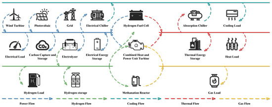
Figure 1.
System structure.
2.1. HCNG-CCS-P2G IES Mathematical Model
2.1.1. HCNG-CCS-P2G Coupled Devices
The HCNG-CCS-P2G system can be divided into two parts: HCNG-CCS and P2G. The HCNG-CCS part is coupled through a Combined Heat and Power (CHP) unit. Hydrogen and natural gas are mixed in a time-varying volumetric ratio to form HCNG, serving as a cleaner fuel for the CHP unit. The carbon emissions produced by combustion are processed by the CCS equipment, as shown in the upper half of Figure 2. This coupling structure efficiently utilizes the gas , improving carbon reduction, tightening the coupling of various energy sources, and reducing energy losses.
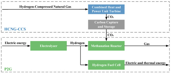
Figure 2.
HCNG-CCS-P2G coupling mechanism.
The expression of the HCNG-CHP model is as follows:
where is the equivalent calorific value of the mixed gas at time t. is the mixed gas power of the CHP at time t.
Considering HCNG, the output power and capacity constraints of electricity and heat from CHP can be expressed as follows:
The modeling of CCS equipment is as follows:
The P2G configuration constitutes another key component of the HCNG-CCS-P2G system, comprising an electrolyzer (EL), a methanation reactor (MR), and a Hydrogen Fuel Cell (HFC). The EL employs grid electricity to perform water electrolysis for hydrogen production. The generated hydrogen is then directed to the MR, where it reacts chemically with the captured by the CCS equipment from CHP emissions, resulting in the production of synthetic natural gas. Additionally, a fraction of the hydrogen produced by the EL can be utilized as fuel for the HFC, converting it into electrical and thermal energy, as illustrated in the lower part of Figure 2. The mathematical models of the three devices are as follows:
2.1.2. DHB Strategy
In the HCNG model, a constraint should be set for the hydrogen blending ratio . Based on whether the blending ratio changes continuously over time or in discrete time phases, the DHB strategy is further divided into two dynamic adjustment strategies: Continuous Hydrogen Blending (CHB) and Time-phased Hydrogen Blending (THB).
The hydrogen blending ratio in CHB changes continuously over time, providing greater flexibility. Therefore, CHB only imposes a range limitation on and solves it as an optimization variable. The range limitation expression is as follows:
where, is the hydrogen blending ratio considering CHB.
In the optimized hydrogen blending ratio, CHB clusters near two specific values during distinct time intervals, exhibiting step characteristics. Furthermore, Reference [20] demonstrated that during the hydrogen blending process, hydrogen fluctuations should be minimized, and hydrogen supply should occur as intermittently as possible. Based on these considerations, the hydrogen blending ratio obtained through CHB optimization is binarized. Specifically, the average value of the 24-h hydrogen blending ratio optimization plan is used as the threshold: for periods below the average, no hydrogen blending is applied (i.e., the blending ratio is zero); for periods above the average, the blending ratio is set to the maximum value (i.e., 20%).
The step characteristics of the hydrogen blending ratio directly reflect the dynamic coupling and economic efficiency of the HCNG-CCS-P2G system. Section 5.2.3 will use simulations to verify the compatibility of this tendency with the THB strategy. Its mathematical model is as follows:
where, is the average value of the CHB hydrogen blending ratio optimization result and is the hydrogen blending ratio considering THB.
2.1.3. Cooling Equipment
This paper considers the combined use of electrical chillers (ECs) and absorption chillers (ACs) to meet the user’s cooling load requirements. Their model is as follows:
2.1.4. Energy Storage Devices
Considering that the models for batteries, thermal storage tanks, and hydrogen storage tanks are similar, this paper uses batteries as an example for modeling:
where, is the energy stored by the energy storage device at time t, is the self-discharge rate of the energy storage device.
2.1.5. Renewable Energy
In this paper, the RES of the IES primarily considers the integration of wind and solar power, which are converted into usable electricity through wind turbines (WTs) and photovoltaic (PV) systems, respectively. Therefore, the power generated by renewable energy in the integrated energy system can be expressed as follows:
2.1.6. Integrated Demand Response
In this paper, the demand response of electricity, heat, cooling, gas, and hydrogen energy is divided into interruptible load and transferable load. The electricity demand response is modeled as follows:
where, is the actual load after IDR at time t.
2.1.7. Constraints
The constraints involved in the IES include the output range limits of each device and energy balance constraints, which are described as follows:
where, is the output of device i at time t.
2.1.8. Carbon Trading Mechanism
Carbon trading consists of carbon emission quotas, actual carbon emissions, and carbon trading rights. The carbon quotas considered in this paper encompass those associated with purchasing electricity from the grid and CHP units. Therefore, the carbon quotas for the IES are modeled as follows:
The carbon emission sources include the grid electricity purchased and CHP. Additionally, MR and CCS also absorb some . Therefore, the actual carbon emissions for the IES are modeled as follows:
2.1.9. Cost Calculation
- (1)
- Carbon Trading Cost
When the actual carbon emissions of the IES exceed their allocated quotas, the system is required to purchase carbon credits from the market, increasing operational costs. To enhance the environmental performance of the IES, a stepped carbon trading mechanism is implemented to regulate actual carbon emissions. The specific model governing this mechanism is detailed as follows:
- (2)
- Integrated Demand Response Cost
Interruptions and load demand transfers inevitably affect user comfort and typically require compensation. For the electricity demand response, the compensation costs are expressed as follows:
- (3)
- Gas and Electricity Purchase Cost
- (4)
- Equipment Operation Cost
For power generation equipment, such as PV and WTs, the operation cost is calculated by multiplying the unit power output by the corresponding operational cost coefficient. For energy coupling devices, such as CHP, EC, AC, EL, MR, HFC, and CCS, their operation cost is calculated by multiplying the corresponding unit energy absorption by the operation cost coefficient. For the three types of energy storage devices, the operation cost is calculated by multiplying the total energy discharged from the storage device by the corresponding operating cost coefficient. The comprehensive expression is as follows:
where, , is the total operation cost, is the operation cost coefficient for the device i.
In summary, the total cost can be expressed as follows:
where, F is the total cost of the integrated energy system.
3. Day-Ahead Distributionally Robust Optimization Model
3.1. Scenario Generation
Prior to performing DRO scheduling, the input data must first be obtained through scenario generation. The uncertainty scenarios include PV and WT generation, as well as five energy loads from the load side. This paper employs a robust distributional optimization model based on data, which requires reducing raw sample data to determine the number and configuration of typical scenarios while ensuring the quality of the results. The correlations in the raw data are first processed using the Latin hypercube sampling (LHS) method. The optimal number and final set of typical scenarios are then determined using the elbow method and K-means clustering.
3.2. Data-Driven Distributionally Robust Framework
Leveraging the distinct characteristics of the various devices, the discrete decision variable representing the state of energy storage is defined as the first-stage variable x. Other continuous decision variables, such as the output levels of different devices, are designated as the second-stage variables . Based on this formulation, the following objective function for uncertainty programming can be established:
where is the probability of the s-th scenario, is the total number of scenarios, and is the set of values that satisfies. The outer layer () makes conservative, first-stage decisions to hedge against the worst-case scenario. The middle layer () identifies the most adverse probability distribution from within an ambiguity set . The inner layer () determines the optimal, second-stage dispatch of devices to minimize costs for any given scenario.
Acknowledging the potential disparity between the initial distribution derived from historical data and the true underlying distribution, the incorporation of ∞-norm and 1-norm constraints is deemed necessary. These constraints are crucial for ensuring that the estimated probability distribution converges to the true probability distribution, especially when a substantial amount of historical data is available. The set is defined as follows:
where, and represent the probability deviation limits corresponding to the 1-norm and ∞-norm constraints, respectively. p is the vector composed of the element .
The probability of the scenarios must satisfy the following confidence constraints:
3.3. Model Solving
The original problem is divided into a master problem (MP) and a subproblem (SP), and the column-and-constraint generation (C&CG) algorithm is used for iterative solving.
- (1)
- MP
The main problem, given the scenario probability distribution p, seeks the optimal solution that satisfies the system’s economy and provides the lower bound for Equation (26):
where, m is the number of iterations.
- (2)
- SP
The subproblem, given the variable in the first stage of the main problem, seeks the worst-case probability distribution under real-time operation, returns it to the main problem, and provides the upper bound for Equation (26):
- (3)
- C&CG Solution Steps
Since the constraints of the master problem and the subproblem are independent, the master problem can be solved first, and then the subproblem can be solved. The specific solving process is as follows:
- Initialization: Set the lower bound , the upper bound . Initialize the iteration counter, say , and utilize the initial probability distribution .
- Master Problem Solution: Solve the MP to obtain the optimal solution . Update the lower bound: .
- Subproblem Solution: Fix the first-stage variable and solve the corresponding subproblem. Obtain the worst-case probability distribution and the value of the objective function . Update the upper bound: .
- Convergence Check: If , terminate the algorithm and return the optimal solution . Otherwise, update the probability distribution for the next iteration , increment the iteration counter , and return to Step 2.
4. Intraday MPC Rolling Optimization
MPC is a model-based closed-loop control method that utilizes the system’s dynamic model to forecast future behavior over a prediction horizon and determines the optimal control input by solving an online optimization problem. The principal variables involved in the MPC formulation include state variables, control variables, and disturbance variables. In this specific application, the output of each device at time t is represented as a state variable vector, denoted by x. The control variables, denoted by u, represent the decisions or actions applied from time t to that govern the system’s evolution. Both the state and control variables are structured into upper and lower layers, and their detailed expressions will be presented in the subsequent section on rolling optimization. Disturbance variables, denoted by , are employed to model uncertainties or external variations, such as fluctuations in renewable energy generation and load demand, at time t. The formulation for these disturbances is given as follows:
MPC consists of prediction models, rolling optimization, and feedback correction. The following section will establish mathematical models for each of these three components.
4.1. Prediction Model
The prediction model is tasked with forecasting the system’s future output values (or states) at each sampling point across a prediction horizon, utilizing the current control input and historical state information. In the context of energy scheduling within this system, the forecasting model is primarily composed of two components: the dynamic transition model for the state variables and the prediction model for the disturbance variables.
where, represents the short-term intraday forecast of at time t, and its value will be provided in Section 5.3.1.
The prediction model incorporates two key parameters: the prediction horizon and the control horizon. The prediction horizon specifies the future period over which system dynamics are forecast, while the control horizon determines the duration during which control actions are optimized and applied. Due to the differing response speeds of the energy carriers—specifically, the rapid dynamics of the electrical load versus the slower transmission of thermal, cooling, gas, and hydrogen loads—a two-layer optimization control strategy is implemented. The upper layer, which manages heat, cooling, gas, and hydrogen loads, operates on a 1-h timescale with both horizons set to 2 h. The lower layer addresses the electrical load at a finer 5-min timescale, with its horizons configured to 1 h.
4.2. Rolling Optimization
The core principle of MPC resides in implementing a rolling optimization strategy. This strategy involves solving an optimization problem over the prediction horizon at each time step to determine an optimal sequence of control actions. However, only the first control action from this sequence is applied to the system. Subsequently, the optimization is repeated in the next time step, incorporating real-time feedback on the system’s state to update the control plan. The specific mathematical model for this rolling optimization process is formulated as follows:
- (1)
- Upper-Layer Model
The upper-layer model involves four types of energy: heating, cooling, gas, and hydrogen. The state variable and control variable are represented as follows:
They also satisfy the state-space Equation (34) in the prediction model. Thus, the standard form of the objective function for the upper-layer MPC optimization model can be established as follows:
where M is the prediction horizon length, is the predicted value of the upper-layer state variable at time given information at time t, and is the control variable relative to the time given information at time . The tracking term, denoted by , minimizes the deviation of state variables from the day-ahead reference schedule, ensuring operational continuity across time steps. The regulation term, expressed as , penalizes the magnitude of control adjustments to prevent aggressive fluctuations and safeguard the operational stability of energy conversion devices.
The constraints mainly include range constraints on state variables, internal coupling constraints, energy storage constraints, and balance constraints. These are expressed as follows:
- (2)
- Lower Layer Model
The lower-layer model is coupled with the upper-layer model. Every hour, the upper layer performs rolling optimization and passes the coupling parameters to the lower-layer model. The variables involved include and . The lower-layer scheduling plans of these variables are directly determined by the upper-layer scheduling strategy based on the coupling relationship. Therefore, the remaining state variables and control variables for the lower layer are expressed as:
The standard form of the objective function for the lower-layer MPC optimization model can be established as
The constraints mainly include range constraints on state variables, energy storage constraints, and electrical balance constraints, which are expressed as follows:
4.3. Feedback Correction
In practical MPC applications, model mismatches and prediction errors can lead to deviations between the rolling optimization results and the actual system states. To mitigate these discrepancies, a dynamic feedback correction mechanism is incorporated. The mathematical model for this mechanism is presented as follows:
where, is the prediction error of the system at time t, is the corrected actual state variable of the system at time , and is the error matrix coefficient.
Based on the principles described above, the step-by-step flow of the MPC is summarized in Figure 3.
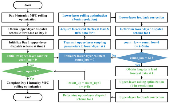
Figure 3.
Two-Layer MPC flowchart.
5. Simulation and Discussion
5.1. Experimental Data and Model Parameters
The strategy proposed in this paper is validated through a case study of a typical single-node IES located in Nanchang, Jiangxi, during the summer season. The optimization model was implemented in MATLAB R2024a utilizing the YALMIP R20230622 toolbox and solved using the GUROBI 11.0.3 solver. All simulations were executed on a computer equipped with 16 GB of RAM and an AMD Ryzen 7 5800H processor (Advanced Micro Devices, Inc., Santa Clara, CA, USA) running at 3.20 GHz.
The configuration parameters and operation cost parameters of each device in the IES are shown in Table 2. The parameters for the stepped carbon trading mechanism are shown in Table 3, the specific data for time-of-use electricity and gas prices are given in Table 4.
Table 2.
Equipment configuration parameters and operational cost coefficients.
Table 3.
Relevant parameters of the stepped carbon trading mechanism.
Table 4.
Time-of-use electricity and gas pricing data.
As described in Section 3.1, 1000 scenarios were initially generated using LHS. Subsequently, the optimal number of clusters was determined to be eight using K-means clustering and the elbow method. Figure 4 illustrates scenarios for the WT and cooling load, serving as representative examples for the RES and load-side scenarios, respectively. Table 5 lists the probabilities and the cost distribution of these eight typical scenarios, illustrating the variations among them.
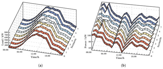
Figure 4.
Day-ahead forecast values of 8 typical scenarios for WT and CL. (a) Cooling Load. (b) Wind Turbine.
Table 5.
Scenario probabilities for 8 typical scenarios and the cost distribution for Case 4.
5.2. Day-Ahead DRO Model Simulation Analysis
5.2.1. Day-Ahead Scheduling Case Studies, Indicators and Analysis Process
To validate the effectiveness of DHB under the day-ahead DRO model, this paper compares the performance of four different strategies in DRO scheduling: no hydrogen blending, fixed optimal hydrogen blending ratio, THB, and CHB strategies. Four cases are analyzed as follows:
Case 1: Use only natural gas as the fuel for CHP in DRO scheduling.
Case 2: Mix natural gas and hydrogen at a fixed volume ratio to optimize the goal for CHP fuel in DRO scheduling.
Case 3: Apply the THB strategy in DRO scheduling.
Case 4: Apply the CHB strategy in DRO scheduling.
In addition, the following seven indicators are used to evaluate the effectiveness of different strategies in day-ahead scheduling: total cost, carbon emissions, carbon trading cost, IDR cost, electricity and gas purchase cost, and operation cost.
It should be noted that the optimal fixed hydrogen blending Ratio for Case 2 has not yet been determined. Therefore, its value will first be established in Section 5.2.2. Subsequently, Section 5.2.3 will provide an initial qualitative analysis of the CHB Ratio distribution pattern. The following sections will then transition to a quantitative analysis, examining the DHB strategy, the DRO method, the system architecture, and key parameters in the scheduling process.
5.2.2. Determining Optimal Fixed Hydrogen Blending Ratio
To determine the optimal value of the fixed hydrogen blending ratio, a sensitivity analysis of the blending ratio r is performed.The blending ratio r is optimized within the range of 0 to 0.2 with a step size of 0.005. Figure 5 shows the relationship between the blending ratio and the total cost. From the magnified dip in the graph, it is clear that when r is set to 0.16, the total cost reaches its minimum value. This indicates that a hydrogen blending ratio of is the optimal choice for scheduling. Therefore, this paper uses 0.16 as the fixed hydrogen blending ratio in Case 2.
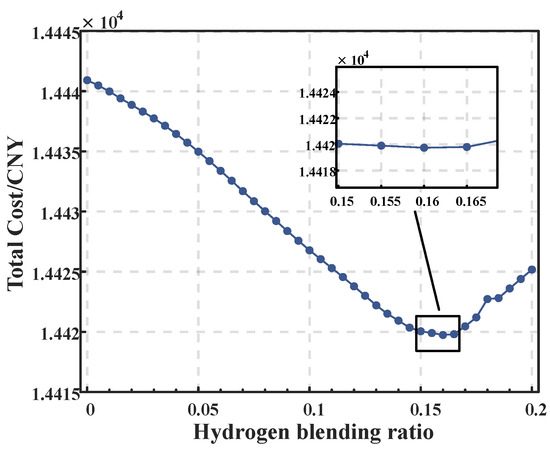
Figure 5.
Sensitivity analysis of hydrogen blending ratio.
5.2.3. CHB Hydrogen Blending Ratio Distribution Pattern
The distribution results of the hydrogen blending ratio r after optimization for Case 4 across eight scenarios are shown in Figure 6. From the figure, it can be seen that the optimized hydrogen blending ratio, r, is concentrated at 0.2 during the 0–7 h and 11–18 h periods and at zero during the 8–10 h and 19–23 h periods. The ratio exhibits a pattern that alternates between two constant values at different times. Furthermore, the hydrogen blending ratio exhibits pronounced step changes across temporal intervals, which further verifies the reasonableness of the THB rule.
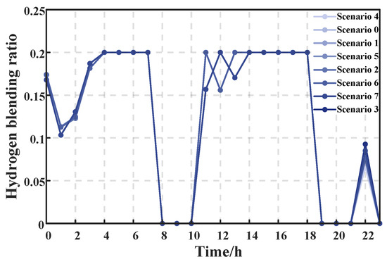
Figure 6.
Distribution of hydrogen blending ratio in Case 4.
The binarized THB strategy significantly simplifies the demands of real-time control. This approach only requires switching the hydrogen blending ratio at predefined time intervals, which is more feasible in practical engineering applications and substantially reduces the design and control complexity of on-site valves and actuators. Such switching operations can be accomplished using the logic of existing industrial control systems, thereby obviating the need for developing high-frequency, high-precision continuous proportional regulation algorithms and hardware. This makes the optimization strategy proposed in this paper more readily implementable in the actual management of integrated energy systems.
5.2.4. Day-Ahead Scheduling DHB Strategy Evaluation
The results of the day-ahead scheduling DHB strategy are presented in Table 6. By comparing the total cost of each case, it can be seen that as the degree of freedom for the hydrogen blending ratio increases, the total scheduling cost gradually decreases. Specifically, compared to Case 1, the total cost of Cases 2, 3, and 4 decrease by 1.07%, 1.84%, and 1.93%, respectively. In Case 4, the CHB strategy resulted in a 0.87% cost reduction compared to the optimal fixed hydrogen blending ratio strategy from Case 2. Given the large base of the total cost, this optimization effect remains significant, indicating that further increasing the freedom of the hydrogen blending ratio plays a crucial role in optimizing system cost.
Table 6.
Evaluation of the day-ahead scheduling DHB strategy.
This optimization effect can be explained theoretically: when the hydrogen blending ratio is fixed, the system’s flexibility is limited and cannot adjust dynamically in response to real-time loads, electricity prices, an other factors. This increases the complexity and cost of scheduling. However, when the hydrogen blending ratio can be dynamically adjusted, the system can flexibly optimize the ratio of natural gas and hydrogen based on load demand and electricity market price fluctuations, thereby optimizing energy production and consumption and reducing unnecessary energy waste. It is this flexibility that leads to the gradual reduction in total scheduling costs.
At the same time, the THB strategy in Case 3 also achieves a cost reduction of 0.79% compared to the optimal fixed hydrogen blending ratio (Case 2). Although it is slightly lower than the CHB strategy, the time-based adjustment method effectively reduces the operational complexity caused by frequent changes in the hydrogen blending ratio. Additionally, adjusting the blending ratio from a variable to a constant avoids generating secondary constraint conditions in the optimization model, reducing the solution time from 60 s to 12 s, an 80% reduction. In practical applications, when considering factors such as model prediction errors, communication delays, and actuator precision, the marginal benefits of pursuing a theoretically continuous optimal solution (CHB) may be limited. In contrast, the simplified scheme offered by THB greatly enhances the feasibility and efficiency of engineering implementation while securing the vast majority of economic benefits. Therefore, for cases emphasizing economic efficiency, the DHB strategy can be considered, while for cases emphasizing engineering simplification and fast scheduling, the THB strategy may be preferred.
However, enhanced operational flexibility may come at the expense of environmental trade-offs. Regarding carbon emissions, although the increased flexibility in the DHB strategy slightly raises carbon emissions, the increase is relatively small. This is mainly due to the constraints of the stepped carbon trading mechanism and the contribution of carbon reduction devices. As shown in Table 6, the increase in carbon trading cost is significant due to the punitive effect of the stepped carbon trading mechanism. Since high carbon emissions face more severe penalties, the system’s carbon emission level has been effectively controlled. Furthermore, the flexible scheduling of CCS and MR helps offset some of the increase in carbon emissions, allowing the system to maintain low carbon emissions while ensuring economic efficiency.
5.2.5. DRO Method Evaluation
To verify the effectiveness of the DRO method, Case 4 is compared with the scheduling results from stochastic optimization (SO) and robust optimization (RO) in the day-ahead phase, as shown in Table 7. From the table, it is evident that the models exhibit varying performance in terms of cost, carbon emissions, and other key indicators. The SO model shows the lowest total cost by assuming probability distributions for uncertainty variables. However, because it relies on historical data to build the probability distribution, it may overlook sudden events, which introduces a higher risk in practical applications. In contrast, the RO model addresses uncertainty by considering the worst-case scenarios. While it ensures system stability, its overly conservative strategy leads to significantly higher total costs than the SO model, resulting in inefficient resource usage and increased operating costs and carbon emissions.
Table 7.
Evaluation of the DRO method.
The DRO model combines the advantages of both SO and RO, effectively addressing uncertainty while avoiding the excessive conservatism of RO and reducing the risks that may arise with SO. The DRO model shows a total cost slightly higher than SO but noticeably lower than RO, indicating that it strikes a better balance between cost and stability while ensuring robustness, demonstrating superior optimization performance.
5.2.6. HCNG-CCS-P2G Structure Evaluation
This section validates the effectiveness of the HCNG-CCS-P2G structure based on the basic hydrogen coupling system (which only includes P2G devices) and sets four system structure scenarios for comparative analysis:
Scenario A: Only considers P2G-related devices (EL, MR, and HFC), without CCS devices and HCNG.
Scenario B: Introduces CCS devices based on Scenario A.
Scenario C: Considers HCNG based on Scenario A.
Scenario D: Uses the HCNG-CCS-P2G structure for the DRO day-ahead scheduling strategy.
The scheduling results are presented in Table 8, which illustrates the impact of various scheduling schemes on the system’s economic performance and low-carbon capabilities. By comparing Scenario A with Scenario B and Scenario C with Scenario D, it can be observed that after introducing CCS (carbon capture and storage) equipment, carbon emissions decreased by 2.68% and 4.30%, respectively, achieving significant emission reduction effects. Furthermore, the emission reduction effect in the IES is more pronounced. The CCS equipment directly reduces the system’s carbon emission by capturing and storing . However, with the introduction of the CCS equipment, the total cost in Scenario A and Scenario C increased by 0.32% and 0.20%, respectively. These cost increases primarily stem from the operational cost of the CCS equipment and its increased energy demand. Nevertheless, considering the substantial reduction in carbon emissions, these additional costs are justified.
Table 8.
Evaluation of the HCNG-CCS-P2G system architecture.
Further comparison between Scenarios A and C, as well as between Scenario B and Scenario D, reveals that with the introduction of HCNG, the CHP system operates more efficiently, resulting in a decrease in total cost of 1.89% and 1.93%, respectively. However, corresponding carbon emissions also increased. This reflects the trade-off between low-carbon performance and economic efficiency. The HCNG-CCS-P2G system combines the economic benefits of HCNG with the effective suppression of carbon emissions through CCS, achieving an ideal integrated outcome.
5.2.7. Norm Constraint Parameter Analysis
In the DRO model, the use of - and -norm constraints is crucial for managing the uncertainties in scenario generation. By adjusting the confidence parameters, the preferences of decision-makers regarding risk can be accommodated. These constraints are used to limit the confidence intervals of the probability distribution, ensuring that the scenario generated remains within a reasonable range, thereby optimizing cost and efficiency while mitigating risks. In this study, simulations were conducted to model a moderate trade-off between system reliability and economic efficiency under the conditions of and . The total scheduling cost under these norm constraints was then compared, as shown in Figure 7.
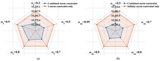
Figure 7.
Norm constraint parameter analysis. (a) 1-norm. (b) Infinity-norm.
As shown in Figure 7, with an increase in the values of and , the total cost gradually rises. This indicates that as these two parameters increase, the optimization model becomes more conservative. Higher values suggest that the model focuses more on dealing with extreme scenarios, and the system adopts more cautious scheduling strategies to reduce risks. This conservative strategy leads to increased use of redundant resources, which results in higher system costs, reflecting the trade-off between risk aversion and cost increase. Therefore, selecting appropriate confidence parameters can flexibly meet the decision-maker’s risk preferences.
Comparing the use of norm constraints individually with the combination of norm constraints, the trend in both figures is consistent: combined norm constraints typically exhibit a lower total cost. For example, in Figure 7b, when , the total cost with combined norm constraints is CNY 15,287, which is lower than the total cost with the use of -norm constraints alone (CNY 15,339). This demonstrates that combined norm constraints can mitigate the cost increase resulting from conservative optimization while ensuring system stability, thereby achieving greater economic efficiency and flexibility, making them more advantageous as DRO constraint conditions.
5.3. Intraday MPC Rolling Optimization Simulation Analysis
5.3.1. Forecast Data Source
Similar to day-ahead scheduling, the main sources of uncertainty are the RES output and the fluctuations in various energy loads. Currently, forecasting methods for renewable energy output and load are well-established, and short-term forecast errors have significantly decreased. Given that the focus of this study is to validate the effectiveness of the DHB strategy, a random error of 5% was added to the day-ahead forecast data to simulate intraday RES and load forecasts. Considering the influence of different timescales, the disturbances of various energy types and loads were adjusted based on their respective timescales. Figure 8 shows the day-ahead forecast data and the intraday ultra-short-term simulation forecast data, with the latter exhibiting higher volatility due to its shorter timescale.
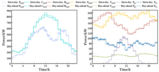
Figure 8.
Simulation forecast data.
5.3.2. Intraday Scheduling Case and Reference Index Setup
Four cases are set for comparative analysis in the intraday scheduling phase to explore the role of CHB in MPC-based intraday scheduling and the effectiveness of the THB under intraday MPC rolling optimization.
Case A: Apply the day-ahead DHB strategy and further adjust the hydrogen blending ratio intraday, followed by MPC rolling optimization.
Case B: Apply the day-ahead DHB strategy and further adjust the hydrogen blending ratio intraday, followed by MPC rolling optimization.
Case C: Maintain the THB hydrogen blending ratio consistent with day-ahead and perform MPC rolling optimization.
Case D: The system is tested using actual intraday forecast data and corresponding forecast errors from a real-world IES demonstration project; the hydrogen blending scheme is consistent with that of Case C.
To conduct a comparative study, six indicators were selected: average solving time, upper-layer tracking error, lower-layer tracking error, upper-layer adjustment cost, lower-layer adjustment cost, and total adjustment cost. The specific definitions are as follows:
Tracking Error:Defined as the difference between the rolling optimization results and the tracking targets, integrated over time throughout the day to quantify the tracking effectiveness of the MPC.
Adjustment Cost: Based on the tracking error, an adjustment cost coefficient is added to quantify the economic performance of the MPC results. The expression is
where, i represents the i-th element in the vector , is the adjustment cost coefficient, is the MPC tracking error, and is the adjustment cost.The adjustment cost coefficient for and is associated with their corresponding and , while the adjustment cost coefficients for other related equipment are equal to their respective operation cost coefficients .
5.3.3. MPC Structure Evaluation
Taking Case B, the most complex scenario in this study, as an example, the solution speed is shown in Table 9. From the listed data, it can be observed that the intraday solution time for the MPC structure reaches the order of seconds, while the day-ahead solution time is at the minute level. After decoupling the timescales, the MPC rolling optimization strategy is faster than the overall DRO optimization, enabling real-time optimization and thereby improving scheduling efficiency, as well as providing better engineering application results.
Table 9.
Multi-timescale methods: speed comparison.
This high computational efficiency suggests that the global optimum is readily found, which in turn ensures precise system tracking. This tracking performance is illustrated in Figure 9 and Figure 10, which, respectively, show the MPC rolling optimization results for the upper-layer and lower-layer models. It can be observed that the trend of changes in the upper-layer coupling variables is consistent, reflecting the constraint effect of the coupling restrictions. It is essential to note that the hydrogen blending ratio, r, which forms the core of the adjustment mechanism, is not tracked like the outputs of the devices but rather optimized as a variable. From the results, it is evident that the trend of r over time is similar to that of the day-ahead forecast, tending toward the boundary values of 0 and 0.2, with a more pronounced step characteristic. This indicates that to mitigate uncertainty error, r will further enhance its characteristics during different periods. When r is low, it will decrease further, and when high, it will increase further, reflecting the reasonableness of the THB strategy.
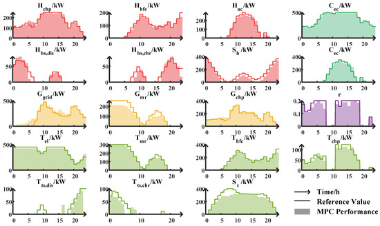
Figure 9.
Upper-layer MPC rolling result.
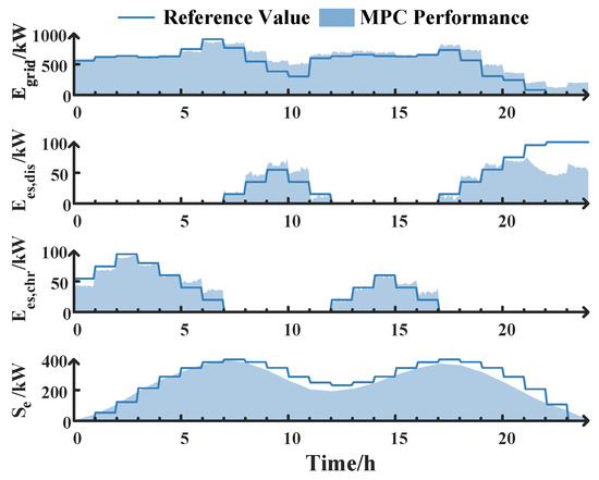
Figure 10.
Lower-layer MPC rolling result.
Additionally, the lower-layer model shows greater tracking deviation compared to the upper-layer model. This is partly because the error from the upper layer propagates to the lower layer, causing cumulative deviations. Furthermore, the lower-layer model has a shorter timescale, and the disturbances designed for it are more frequent.
Overall, the MPC structure effectively integrates system states with day-ahead optimization results during intraday rolling optimization, maintaining the system’s stability and optimization effectiveness. Through this approach, MPC not only responds quickly to real-time data but also ensures that the long-term goals of the system are consistent with the day-ahead plan, improving the overall scheduling performance.
5.3.4. Intraday Scheduling DHB Strategy Evaluation
The results for the three cases are shown in Table 10. Comparing Case A and Case B, it is evident that further adjusting the hydrogen blending ratio r during the intraday period leads to a decrease in the upper-layer and lower-layer tracking error based on CHB by 4.25% and 2.3%, respectively, indicating that this strategy enables MPC to track the targets more accurately. However, this strategy is accompanied by a certain increase in adjustment cost. In Case B, although the total adjustment cost increased by 0.84% compared to Case A, the improvement in tracking precision due to the adjustment of the blending ratio requires a balance between controlling error and controlling cost. For better tracking performance, further dynamic adjustment of the hydrogen blending ratio during the day is an ideal choice, with the slight increase in total adjustment cost being acceptable.
Table 10.
Evaluation of the intraday scheduling DHB strategy.
Compared to Case A, although CHB exhibits some advantages in the upper-layer tracking error metric, the transmission of coupling parameters between layers leads to an increase in the lower-layer tracking error due to excessive tracking in the upper layer, indirectly elevating the total tracking error. In contrast, Case C, when adjusting the hydrogen blending ratio, can mitigate lower-layer fluctuations, achieving a superior lower-layer tracking performance, with a reduction in the lower-layer tracking error of 2.43%. Considering the shorter timescale and greater uncertainty fluctuations in the lower-layer model, this indicates that THB demonstrates better intraday tracking performance under these circumstances.This result also corroborates that the THB strategy aligns more closely with the hierarchical control architecture of practical systems. The upper layer (operating on a longer timescale) is responsible for formulating relatively stable operational plans. In comparison, the lower layer (operating on a shorter timescale) focuses on rapid fluctuation suppression and precise tracking.
The comparison of cost contrasts with the trends in tracking error. In terms of cost optimization, CHB performs better in the overall economy, particularly in upper-layer adjustment costs, while the lower-layer economy is still inferior to THB. Therefore, when emphasizing long timescale scheduling issues, the CHB strategy achieves a good balance between tracking precision and economic performance, ensuring that the system operates efficiently. For short timescale power scheduling issues, THB’s advantages are more prominent. For the overall IES, CHB is more suitable for long-term scheduling scenarios with higher economic requirements and sufficient computational resources, ensuring tracking performance within a certain range. In contrast, THB is more suited to stabilizing the tracking of day-ahead scheduling strategies, especially for scenarios that emphasize scheduling stability and operational convenience.
A comparison between Case D (using real-world data) and Case C (using simulated data) reveals that the metrics, while showing some variation, are largely comparable. This is attributed to the fact that although the actual fluctuation patterns of renewable generation and various energy loads differ between the cases, the forecast error levels of the data employed are similar. These results demonstrate the proposed model’s robustness in the face of different uncertainty profiles. Furthermore, they corroborate the practical feasibility of the proposed MPC framework and THB for real-world applications.
6. Conclusions
This study establishes an HCNG-CCS-P2G system and combines day-ahead DRO and intraday MPC rolling optimization methods to explore the adjustment effects of DHB in the day-ahead–intraday scheduling of the IES, aiming for the robust and economic operation of the IES. The simulation results verify the effectiveness of the proposed strategies, with the findings summarized as follows:
- HCNG-CHP, as an integration of electricity, heat, gas, and hydrogen, possesses strong adjustment capabilities. For the day-ahead system DRO scheduling, the DHB strategy achieved a 0.87% reduction in total cost compared to the traditional fixed hydrogen blending ratio. This provides system operators with a direct and quantifiable method to improve the profitability and flexibility of complex, multi-energy systems.
- The THB strategy, proposed based on dynamic hydrogen blending with step characteristics, simplifies the secondary constraints of the dynamic hydrogen blending model in intraday scheduling. This not only reduces costs but also reduces the solving time by 80%, making it a good engineering approximation of CHB. This significant reduction in computational demand bridges the gap between theoretically optimal models and the fast-response requirements of live industrial control systems, making real-world implementation feasible.
- In improving the tracking performance of intraday MPC rolling optimization, further adjustment of the hydrogen blending ratio during the day led to a decrease in upper-layer and lower-layer tracking errors by 4.25% and 2.37%, respectively. This indicates that dynamic hydrogen blending can more effectively track the day-ahead scheduling plan, achieving a balance between economy and robustness. This leads to a more robust and stable energy system, minimizing costly deviations from dispatch plans and enhancing the reliability of energy delivery.
- Compared to CHB, THB demonstrates a more pronounced effect on power regulation at shorter timescales, leading to a 2.43% reduction in the lower-layer tracking error. This suggests that THB can effectively minimize the tracking error propagated from the upper layer to the lower layer within the MPC framework. Conversely, CHB is better suited for adjusting energy types over longer time horizons. This finding serves as a functional user guide for system operators, enabling them to select the optimal control strategy that effectively balances real-time stability with long-term economic efficiency.
Author Contributions
Conceptualization, Y.X. and X.Y.; methodology, Y.X.; software, Y.X.; validation, Y.X., Q.X. and K.W.; formal analysis, K.W.; investigation, Y.Z.; resources, X.Y.; data curation, K.W.; writing—original draft preparation, Y.X.; writing—review and editing, Q.X.; visualization, K.W.; supervision, X.Y.; project administration, Q.X. All authors have read and agreed to the published version of the manuscript.
Funding
This research received no external funding.
Institutional Review Board Statement
Not applicable.
Informed Consent Statement
Not applicable.
Data Availability Statement
The data presented in this study are available on request from the corresponding author.
Conflicts of Interest
The authors declare no conflicts of interest.
Nomenclature
| chp | Combined Heat and Power |
| pv | Photovoltaic |
| wt | Wind turbine |
| el | Electrolyzer |
| mr | Methanation reactor |
| hfc | Hydrogen Fuel Cell |
| ccs | Carbon Capture and Storage |
| ec | Electrical chiller |
| ac | Absorption chiller |
| es | Electrical energy storage |
| hs | Thermal energy storage |
| ts | Hydrogen storage |
| dis | Discharge |
| chr | Charge |
| tra | Transferable load |
| int | Interruptible load |
| gas | Natural gas |
| ref | Reference value |
| up | Upper layer model |
| low | Lower layer model |
| min | Minimum |
| max | Maximum |
| P | Electrical energy |
| H | Heat energy |
| C | Cooling energy |
| G | Gas energy |
| T | Hydrogen energy |
| M | Mixed gas energy |
| r | Hydrogen blending ratio |
| L | Calorific value |
| Carbon dioxide | |
| f | Cost |
| Q | Weight coefficient matrix for state variables |
| R | Weight coefficient matrix for control variables |
| Equipment operating efficiency | |
| Carbon emission coefficient | |
| Electrical-to-Thermal conversion efficiency | |
| Proportion | |
| Basic carbon trading price | |
| Increasing coefficient of carbon trading price | |
| l | Interval length of carbon trading price segmentation |
| IDR cost coefficient | |
| c | Operation cost coefficient |
| s | Index of scenario |
References
- Hassan, Q.; Viktor, P.; Al-Musawi, T.J.; Ali, B.M.; Algburi, S.; Alzoubi, H.M.; Al-Jiboory, A.K.; Sameen, A.Z.; Salman, H.M.; Jaszczur, M. The renewable energy role in the global energy Transformations. Renew. Energy Focus 2024, 48, 100545. [Google Scholar] [CrossRef]
- Kamali Saraji, M.; Streimikiene, D. Challenges to the low carbon energy transition: A systematic literature review and research agenda. Energy Strateg. Rev. 2023, 49, 101163. [Google Scholar] [CrossRef]
- Liu, Z.; Fan, G.; Meng, X.; Hu, Y.; Wu, D.; Jin, G.; Li, G. Multi-time scale operation optimization for a near-zero energy community energy system combined with electricity-heat-hydrogen storage. Energy 2024, 291, 130397. [Google Scholar] [CrossRef]
- Rolo, I.; Costa, V.; Brito, F. Hydrogen-Based Energy Systems: Current Technology Development Status, Opportunities and Challenges. Energies 2023, 17, 180. [Google Scholar] [CrossRef]
- Zhu, L.; Wang, J.; Tang, L.; Liu, S.; Huang, C. Robust Stochastic Optimal Dispatching of Integrated Energy Systems Considering Refined Power-to-Gas Model. Power Syst. Technol. 2019, 43, 116–125. [Google Scholar] [CrossRef]
- He, L.; Lu, Z.; Zhang, J.; Geng, L.; Zhao, H.; Li, X. Low-carbon economic dispatch for electricity and natural gas systems considering carbon capture systems and power-to-gas. Appl. Energy 2018, 224, 357–370. [Google Scholar] [CrossRef]
- Ma, Y.; Wang, H.; Hong, F.; Yang, J.; Chen, Z.; Cui, H.; Feng, J. Modeling and optimization of combined heat and power with power-to-gas and carbon capture system in integrated energy system. Energy 2021, 236, 121392. [Google Scholar] [CrossRef]
- Wang, J.; Mao, J.; Hao, R.; Li, S.; Bao, G. Multi-energy coupling analysis and optimal scheduling of regional integrated energy system. Energy 2022, 254, 124482. [Google Scholar] [CrossRef]
- Liang, Y.; Wang, Y.; Liu, H.; Wang, P.; Jing, Y.; Li, J. Optimal Operation of Integrated Energy System Considering Demand Response. J. Phys. Conf. Ser. 2021, 2087, 012017. [Google Scholar] [CrossRef]
- Qadrdan, M.; Abeysekera, M.; Chaudry, M.; Wu, J.; Jenkins, N. Role of power-to-gas in an integrated gas and electricity system in Great Britain. Int. J. Hydrogen Energy 2015, 40, 5763–5775. [Google Scholar] [CrossRef]
- Wei, Z.; Li, J.; Yang, C.; Zhang, Z.; Yuan, K.; Pan, R. Low-carbon Economic Scheduling for Integrated Energy System Based on Dynamic Hydrogen Doping Strategy. Power Syst. Technol. 2024, 48, 3155–3164. [Google Scholar] [CrossRef]
- Zakaria, A.; Ismail, F.B.; Lipu, M.H.; Hannan, M. Uncertainty models for stochastic optimization in renewable energy applications. Renew. Energy 2020, 145, 1543–1571. [Google Scholar] [CrossRef]
- Ruan, Y.; Qian, F.; Sun, K.; Meng, H. Optimization on building combined cooling, heating, and power system considering load uncertainty based on scenario generation method and two-stage stochastic programming. Sustain. Cities Soc. 2023, 89, 104331. [Google Scholar] [CrossRef]
- Shen, F.; Zhao, L.; Wang, M.; Du, W.; Qian, F. Data-driven adaptive robust optimization for energy systems in ethylene plant under demand uncertainty. Appl. Energy 2022, 307, 118148. [Google Scholar] [CrossRef]
- Zhou, Y.; Wei, Z.; Shahidehpour, M.; Chen, S. Distributionally Robust Resilient Operation of Integrated Energy Systems Using Moment and Wasserstein Metric for Contingencies. IEEE Trans. Power Syst. 2021, 36, 3574–3584. [Google Scholar] [CrossRef]
- Pourahmadi, F.; Kazempour, J. Distributionally Robust Generation Expansion Planning With Unimodality and Risk Constraints. IEEE Trans. Power Syst. 2021, 36, 4281–4295. [Google Scholar] [CrossRef]
- Li, Y.; Han, M.; Shahidehpour, M.; Li, J.; Long, C. Data-driven distributionally robust scheduling of community integrated energy systems with uncertain renewable generations considering integrated demand response. Appl. Energy 2023, 335, 120749. [Google Scholar] [CrossRef]
- Ma, M.; Lou, C.; Xu, X.; Yang, J.; Cunningham, J.; Zhang, L. Distributionally robust decarbonizing scheduling considering data-driven ambiguity sets for multi-temporal multi-energy microgrid operation. Sustain. Energy Grids Netw. 2024, 38, 101323. [Google Scholar] [CrossRef]
- Yang, X.; Wang, X.; Leng, Z.; Deng, Y.; Deng, F.; Zhang, Z.; Yang, L.; Liu, X. An optimized scheduling strategy combining robust optimization and rolling optimization to solve the uncertainty of RES-CCHP MG. Renew. Energy 2023, 211, 307–325. [Google Scholar] [CrossRef]
- Zhou, J.; Jiang, X.; Li, S.; Zhu, J.; Zhou, Z.; Liang, G. Operation optimization for gas-electric integrated energy system considering hydrogen fluctuations and user acceptance. Int. J. Hydrogen Energy 2024, 88, 666–687. [Google Scholar] [CrossRef]
Disclaimer/Publisher’s Note: The statements, opinions and data contained in all publications are solely those of the individual author(s) and contributor(s) and not of MDPI and/or the editor(s). MDPI and/or the editor(s) disclaim responsibility for any injury to people or property resulting from any ideas, methods, instructions or products referred to in the content. |
© 2025 by the authors. Licensee MDPI, Basel, Switzerland. This article is an open access article distributed under the terms and conditions of the Creative Commons Attribution (CC BY) license (https://creativecommons.org/licenses/by/4.0/).