Analysis of Weak Links in the Mechanized Mining of Underground Metal Mines: Insights from Machine Learning and SHAP Explainability Models

Abstract

In the mechanized mining of metal mines, identifying and optimizing vulnerabilities within the production system is essential for enhancing operational efficiency and ensuring sustainable development. By leveraging data from 88 stopes at Guangxi Tongkeng Mine over a decade, we constructed a comprehensive dataset encompassing drilling, charging, blasting, ventilation, support, ore drawing, and maintenance. The XGBoost algorithm was employed to model factors influencing stope production capacity (PC), with its parameters optimized using the Marine Predator Algorithm (MPA). The MPA–XGBoost model demonstrates a high predictive accuracy for PC (R² = 0.958, VAF = 95.981%, MAE = 4.844, RMSE = 7.033). A Shapley Additive Explanations (SHAP) analysis reveals that drilling efficiency (DE) contributes most positively (35.6%), while ventilation time (VT) and equipment maintenance time (EMT) negatively impact PC. SHAP dependence plots indicate that increasing DE significantly enhances PC, whereas excessive VT or EMT leads to a substantial decline in PC. These findings offer valuable insights and a robust foundation for optimizing design and improving production management in mechanized mining operations.

1. Introduction

Underground mining is a typical multi-process operation [1]. The design of mining methods generally encompasses processes such as rock drilling, blasting, ventilation, support, and ore drawing, requiring the coordination of multiple types of workers and equipment [2]. The inefficient management of production processes can not only reduce production efficiency but also potentially introduce safety hazards in mining operations.

In the past few decades, mines have predominantly adopted an extensive management model. This was primarily due to the relatively favorable mining environments of ore bodies in the past. The ore bodies were typically thick, large, and high-grade, and government regulations regarding mine safety control were less stringent. Mines could achieve high profits without implementing fine-grained management practices. Additionally, the mechanization level of mine production was relatively low in the past. The management process heavily relied on person-to-person communication, which hindered the realization of refined management across the entire production process [3,4,5].

With the increasing mining depth of ore bodies, the emergence of high-temperature and high ground pressure conditions has rendered the mining environment increasingly harsh, thereby escalating the risk factors associated with human operations [6,7,8]. Alongside the advancement of mechanization, modern mines have started to employ mechanized equipment to replace traditional manual operations across various production processes [9]. During normal production in modern mines, the extensive application of mechanized equipment, particularly within the framework of mine intelligence, implies that production efficiency is predominantly determined by the performance of mechanized equipment, stope geological conditions, and the design of the mining system [10,11,12,13].

For instance, in the rock drilling process, the efficiency of rock drilling equipment is of critical importance [14]. Both drilling speed and equipment failure rates substantially influence the efficiency of the rock drilling process. When encountering fractured rock formations, rock drilling equipment is highly susceptible to jamming during operation, leading to a significant reduction in drilling efficiency. Furthermore, the design of the mining system is of paramount significance [15]. In practical mining operations, it is imperative to conduct timely ventilation, cooling, drainage, and support based on engineering conditions to ensure the safety of mining activities. These factors constitute fundamental considerations in the design of the mining system and directly affect production efficiency [16].

The evolving production environment and shifting management objectives have necessitated that mine production managers enhance the refined management of the entire process. The relevant personnel must carry out in-depth analyses of underground metal mine operations, identify weak links in the mining process, and implement more scientific optimization systems and effective measures to address these issues. Numerous scholars have conducted research on optimizing the production process of underground metal mines using mathematical programming methods. In 2010, Micah Nehring et al. [17] proposed a new mixed-integer programming (MIP) model that significantly reduced the solution time for underground mine production scheduling problems while maintaining result accuracy and satisfying all constraint conditions. In 2020, Farzad Sotoudeh et al. [18] comprehensively reviewed the application of mathematical programming in the production scheduling optimization of sub-level open-stoping mines, providing recommendations for future research and highlighting the crucial role of such methods in optimizing complex systems. In 2023, E. J. A. Appia Ning et al. [19] applied a mixed-integer linear programming framework to comprehensively optimize the development and production scheduling of open-pit mines, aiming to maximize mine life. Shuwei Huang et al. [20] constructed an optimization framework for backfill mining production scheduling using mixed-integer linear programming. Additionally, in 2019, Liu Di et al. [21] proposed a boundary grade optimization model for underground polymetallic mines, further expanding the application scope of Lane’s theory. These studies have made substantial contributions to enhancing the production efficiency of underground metal mines, reducing costs, and promoting sustainable development through the application of various mathematical programming methods. They offer valuable theoretical and practical references for tackling challenges in the production process.

Although mathematical programming methods have achieved remarkable results in optimizing the production process of underground metal mines, they also possess certain limitations. Firstly, these methods typically depend on precise mathematical models and well-defined constraint conditions. However, the actual production process is highly complex, involving numerous uncertain factors, which makes it challenging to construct an accurate model using purely mathematical approaches. As a result, the model may not fully align with real-world scenarios, thereby impacting the accuracy and practicality of the optimization outcomes. Secondly, when addressing large-scale and high-dimensional problems, the computational complexity of mathematical programming methods increases substantially, leading to significantly extended solution times. This limitation restricts their applicability in more intricate production environments.

In contrast, machine learning methods exhibit distinct advantages in production process optimization [22]. Machine learning methods can automatically uncover potential patterns and rules in data by learning from a substantial volume of actual production data, without the necessity of pre-constructing an accurate mathematical model [23,24]. They demonstrate stronger adaptability to complex and highly uncertain production environments. When handling large-scale data, machine learning algorithms can efficiently conduct data analysis and processing with the support of technologies such as distributed computing, significantly reducing calculation time and enhancing optimization efficiency [25]. Moreover, machine learning models possess excellent adaptability and dynamic learning capabilities, enabling them to update and optimize the model in real time based on newly generated data. This allows the models to promptly adapt to various changes in the production process and effectively meet the demands of continuous production process optimization [26].

To further investigate the weak links in the underground mining system, this study gathered data from 88 stopes in Tongkeng Mine, Guangxi Province, China, over a decade to construct a comprehensive dataset. By employing machine learning techniques, this study incorporated the key influencing factors of the mining system, established an accurate regression analysis relationship with the production capacity of the mining system, and utilized the SHAP interpretability model to rank and compare the influencing factors regarding the production capacity of the mining system. The objective was to identify the weak links in stope mining efficiency and provide critical insights for the adaptive adjustment of stope mining technology.

2. Materials

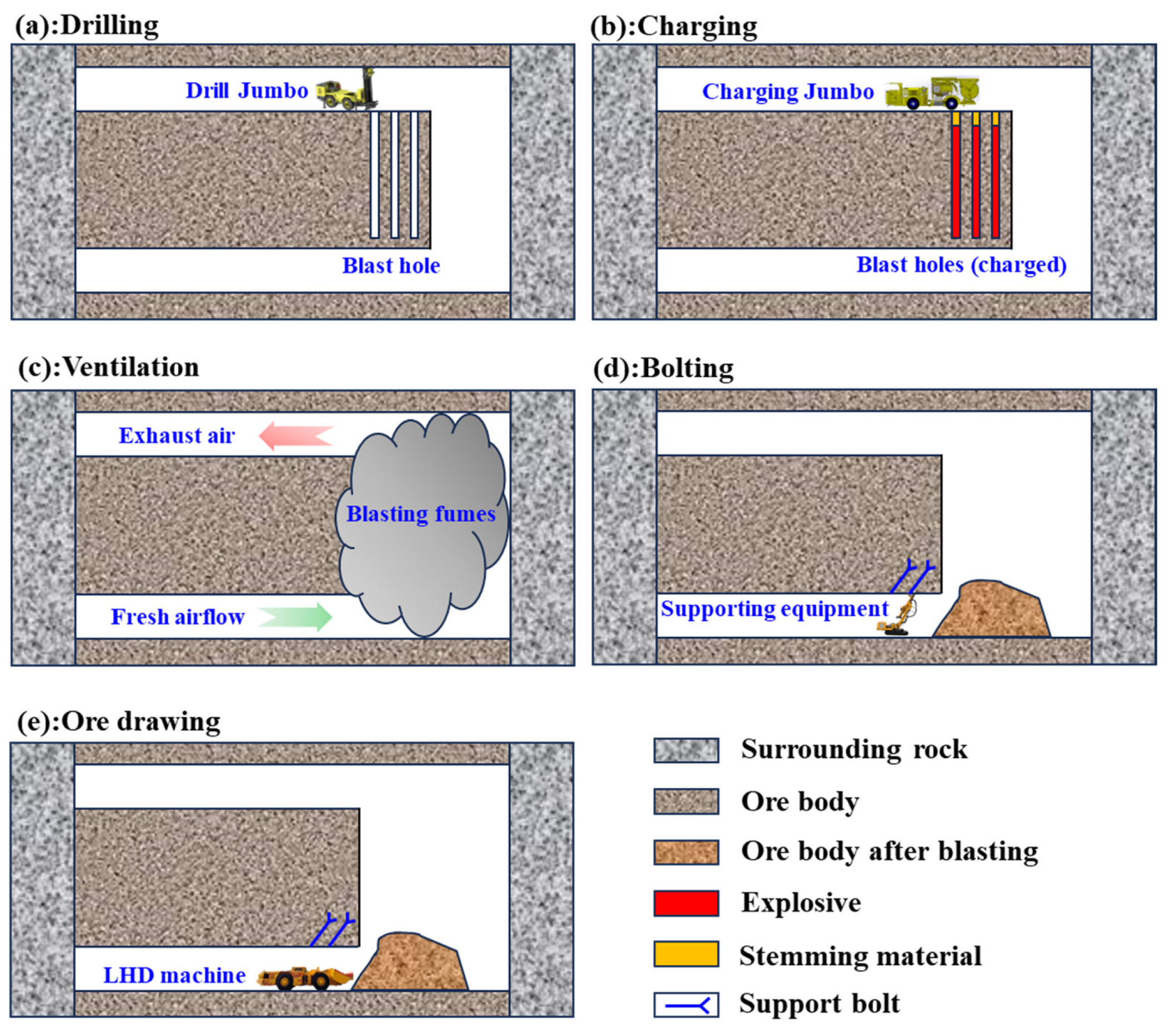
2.1. Mechanized Mining Processes

In mines where mechanized mining is extensively applied, the medium and deep hole mining method is predominantly adopted [27], as illustrated in Figure 1. Ore body mining constitutes a multi-process task, primarily encompassing rock drilling, charging, blasting, ventilation, support, ore drawing, and other operations. For a mining area, during the initial design phase, geological engineers can estimate the Designed Ore Mining Quantity (DOMQ/t). The production capacity (PC/(t/d)) is employed as a metric to evaluate the mining efficiency and production capacity of the stope. The key factors influencing the stope’s mining efficiency and production capacity at different stages are outlined below:

(1)

During the drilling stage, workers are required to operate the drilling rig to drill blast holes in accordance with the mining design. Given that the blast hole depth in medium and deep hole mining typically exceeds 15 m, the primary factor influencing mining efficiency at this stage is the drilling efficiency (DE, m/d).

(2)

In the charging stage, engineers utilize the charging jumbo to charge and detonate explosives within the blast holes. The charging and blasting efficiency (CBE, h/d) serves as the main influencing factor during this phase.

(3)

Following the blasting process, a significant amount of fumes is generated in the blasting area, necessitating ventilation for dispersion. In mines with an inefficient ventilation system, the ventilation time (VT, h/d) may exceed 12 h, thereby substantially impacting production efficiency.

(4)

In the support stage, due to rock mass damage caused by blasting, support operations become critical. If the surrounding rock is unstable, additional time will be allocated for support work. The support time (ST, h/d) constitutes the primary influencing factor during this stage.

(5)

In the ore drawing stage, loaders are employed to shovel, transport, and unload the blasted ore. The ore removal efficiency (ORE, t/d) represents the main factor affecting mining efficiency at this stage.

(6)

It is worth noting that in mechanized mines, the equipment maintenance time (EMT, d) of mining equipment cannot be overlooked, as it also plays a significant role in influencing production efficiency [28].

2.2. Dataset Construction

Regarding the influencing factors of modern mining technology, we aggregated the PC statistics from 88 stope mines post mining. Subsequently, based on these factors, we systematically collected data on DOMQ, DE, CBE, VT, ST, ORE, and EMT for these 88 mines, thereby constructing an initial dataset. The data were sourced from the mining records of Tongkeng Mine in Guangxi, China, spanning over a decade. As illustrated in Figure 2, the data for each factor exhibit significant dispersion. This complexity highlights the challenges of using traditional linear mathematical methods to accurately capture their relationships, thereby underscoring the necessity of employing machine learning techniques.

A correlation matrix analysis was performed on the constructed dataset (Figure 3). From the scatter plots of data associations in the lower triangle of the correlation matrix diagram, it is clear that the data exhibit strong discreteness, with no apparent linear correlations among the factors. This phenomenon arises because different stope mines differ significantly in terms of ore body shapes and surrounding rock conditions, resulting in varying mining outcomes. The central data distribution in the diagram reveals that most factors generally follow a normal distribution, except for ST, which follows an exponential distribution. Given the relatively stable surrounding rock in the mines providing the data, the short support time in the stope leads to this specific distribution pattern of ST data. In the upper triangle portion of the correlation matrix diagram, the correlation coefficients indicate that DE, ORE, CE, and DOMQ are positively correlated with PC (correlation coefficient > 0), with DE showing a strong positive correlation (0.9). Conversely, VT, ST, and EMT are negatively correlated with PC (correlation coefficient < 0), with VT and EMT exhibiting strong negative correlations (−0.843 and −0.831). However, the correlation analysis can only reveal the relationship between individual factors and PC. To comprehensively understand the correlation characteristics between multiple factors and PC, it is essential to employ machine learning methods to construct a regression analysis model.

3. Methodology

3.1. Extreme Gradient Boosting (XGBoost)

To explore the complex regression relationship between the multi-dimensional factors and PC (the target variable), this study adopts the Extreme Gradient Boosting (XGBoost) algorithm [29]. XGBoost is developed based on the Gradient Boosting Decision Tree (GBDT) framework and iteratively optimizes weak regression or classification models, constructing a robust predictive system. By incorporating parallel computing techniques, it efficiently handles large-scale datasets, thereby substantially reducing training time.

Theoretically, XGBoost exhibits superior performance in both classification and regression tasks. By leveraging the second-order Taylor expansion of the loss function, it captures nonlinear relationships more accurately, thereby enhancing prediction accuracy. This capability has enabled XGBoost to be widely applied across various domains, including financial risk assessment, medical diagnosis, and industrial fault detection [30].

In this study, XGBoost integrates regularization terms into the objective function optimization process. This not only controls model complexity but also alleviates overfitting by penalizing excessively large weights, thereby enhancing generalization performance. XGBoost acts as a fast and reliable tool for complex simulations. Its data prediction mechanism constructs an ensemble model through iterative residual fitting, as shown in Equation (1).

$$Ob{j}^{(r)}={\displaystyle \sum _{i=1}^{m}L({\mathrm{y}}_i,{\widehat{\mathrm{y}}}_i^{(r)})}+{\displaystyle \sum _{k=1}^r\mathsf{\Omega }(g_r)}$$

(1)

In this equation, y_i represents the measured value, ${\widehat{y}}_i^{(r)}$ representing the r-th prediction result, g_r is the term of the decision tree, $L({\mathrm{y}}_i,{\widehat{\mathrm{y}}}_i^{(\mathrm{r})})$ representing the loss function, and the regularized term Ω(g_r) is given by Equation (2):

$$\mathsf{\Omega }(g_r)=\gamma \mathrm{T}+{\displaystyle \frac{1}{2}}\lambda {\displaystyle \sum _j^T{w}^2}$$

(2)

In Equation (2), T denotes the root node of the decision tree, while w indicates the weight associated with each root node. The default values for the coefficients λ and γ are set to λ = 1 and γ = 0, respectively.

In practical applications, the performance of the XGBoost regression model is highly dependent on the optimal configuration of key parameters [31]. As shown in

Table 1. XGBoost calculation parameters.

Parameters	Parameter Description	Data Range
num_trees	This parameter plays a crucial role in assessing the model’s predictive performance. Generally, a higher value enhances learning and data processing capabilities, resulting in more accurate predictions. However, an excessively high value may lead to the inefficient utilization of computational resources, thereby diminishing overall efficiency.	[1, 1000]
max_depth	This parameter, which specifies the maximum depth of the decision tree, plays a critical role in controlling overfitting. Although larger values allow the model to capture more complex patterns and improve training performance, they also increase the risk of overfitting, thereby compromising the model’s ability to generalize to new data.	[1, +∞]
eta	This parameter determines the step size for each iteration and plays a pivotal role in influencing algorithm performance. Setting the value too high may degrade the algorithm’s precision, while an excessively low value will significantly prolong execution time. Both scenarios can adversely affect the algorithm’s overall effectiveness, thereby highlighting the importance of carefully adjusting this parameter to achieve an optimal balance.	[0.01, 0.1]

, num_trees, max_depth, and eta act as the core control parameters of the model, and their values directly affect the model’s fitting capacity and generalization ability. Although traditional manual parameter tuning can improve model performance to some extent, this approach is constrained by human experience and subjective judgment. It not only tends to introduce bias but also risks, causing the model to converge to a local optimum rather than achieving a globally optimal parameter configuration, thereby impacting the accuracy and reliability of the regression analysis.

3.2. Marine Predators Algorithm (MPA)

To achieve the efficient and precise optimization of the XGBoost algorithm’s parameters, this study utilized the Marine Predators Algorithm (MPA) [32]. Proposed by Afshin Faramarzi et al. in 2020 [33], MPA draws inspiration from the foraging behavior of marine predators. Specifically, the algorithm incorporates the Lévy flight and Brownian motion patterns observed in marine predators. Lévy flight is characterized by occasional long-distance jumps and frequent short-distance movements, enabling predators to search for prey efficiently in vast ocean environments. Brownian motion reflects the random displacement of particles in fluids, simulating the unpredictable movement of prey. Furthermore, MPA simulates the optimal encounter rate strategy between predators and prey, where predators adjust their behaviors to maximize encounter probability while minimizing energy expenditure [34]. This study demonstrates the application of MPA, offering novel insights into optimizing XGBoost parameters.

The optimization process of the MPA comprises three key stages, as shown in Figure 4. In each specified stage, a corresponding number of iteration cycles is assigned. These steps are determined according to the rules governing predator–prey movements and mimic the behavioral patterns of predators and prey in natural ecosystems.

(1) In the beginning, akin to most meta-heuristic algorithms, the MPA randomly determines the initial positions of the prey within the search space to start the optimization procedure. The mathematical representation is as follows:

$$X_0 =X_{min} +rand(X_{max} -X_{min} )$$

(3)

where X_max and X_min denote the upper and lower bounds of the search space, respectively, while rand () represents a random number generated within the interval [0, 1].

(2) During the initial stages of the iteration, the speed of the predator exceeds that of the prey. Consequently, the MPA employs an exploration strategy, which is mathematically formulated as follows:

$$\left\{\begin{array}{l}stepsiz{e}_i =R_B\otimes (Elit{e}_i -R_B\otimes Pre{y}_i )\\ Pre{y}_i =Pre{y}_i +0.5\times R\otimes stepsiz{e}_i\end{array}\right. i=1,2,3....,n. Iter<{\displaystyle \frac{Max\_Iter}{3}}$$

(4)

where stepsize_i represents the step length of movement; R_B is a random vector of Brownian motion distributed normally; Elite_i is an elite matrix constructed by the top predator; Prey_i is a matrix of the same dimension as the elite matrix; R is a uniformly random vector within [0,1]; n is the swarm size; and Iter and Max_Iter represent the current and maximum number of iterations, respectively.

(3) During the intermediate stage of the iteration, when the speeds of predators and prey are equal, the prey employs the Lévy flight strategy for exploitation, while the predators utilize the Brownian motion strategy for exploration. Over time, the predators gradually transition from an exploration-focused approach to an exploitation-focused approach. The mathematical formulations for both exploitation and exploration are as follows:

$$\left\{\begin{array}{l}stepsiz{e}_i =R_L\otimes (Elit{e}_i -R_L\otimes Pre{y}_i )\\ Pre{y}_i =Pre{y}_i +0.5\times R\otimes stepsiz{e}_i\end{array}\right. i=1,2,3....,n/2.\hspace{0.33em}{\displaystyle \frac{Max\_Iter}{3}}<Iter<{\displaystyle \frac{2Max\_Iter}{3}}$$

(5)

$$\left\{\begin{array}{l}stepsiz{e}_i =R_B\otimes (R_B\otimes Pre{y}_i -Elit{e}_i )\\ Pre{y}_i =Elit{e}_i+0.5\times CF\otimes stepsiz{e}_i\end{array}\right. i=n/2,....,n.\hspace{0.33em}{\displaystyle \frac{Max\_Iter}{3}}<Iter<{\displaystyle \frac{2Max\_Iter}{3}}$$

(6)

where R_L is a random vector that follows the Lévy distribution; CF is an adaptive parameter controlling the step length of the predator’s movement; and the meanings of the other parameters are consistent with those described previously.

(4) During the latter stages of the iterative process, when the movement speed of the predator lags behind that of the prey, the Marine Predator Algorithm (MPA) implements a development (exploitation) strategy. In this phase, the predator utilizes the Lévy flight strategy. The mathematical formulation for this approach is presented below:

$$\left\{\begin{array}{l}stepsiz{e}_i =R_L\otimes (Elit{e}_i -R_L\otimes Pre{y}_i )\\ Pre{y}_i =Pre{y}_i +0.5\times R\otimes stepsiz{e}_i\end{array}\right. i=1,2,3....,n. Iter>{\displaystyle \frac{2Max\_Iter}{3}}$$

(7)

(5) To incorporate the FADs effect, this mechanism is designed to prevent stagnation at local optima. The equation for this approach is described as follows:

$$Pre{y}_{i }=\left\{\begin{array}{l}Pre{y}_i +CF[X_{min }+R\otimes (X_{max} -X_{min })]\otimes U,\hspace{0.33em}r\le FADs\\ Pre{y}_i +[FADs(1-r)+r](Pre{y}_{r_1} -Pre{y}_{r_2}), r>FADs\end{array}\right.$$

(8)

Among them, FADs denote the probability influencing the optimization process of the algorithm and are typically set to 0.2; U is a binary vector sequence randomly generated with elements of 0 or 1; R is a random number within the interval [0, 1]; and r₁ and r₂ are random indices of the prey matrix.

3.3. Prediction Evaluation Indicators

In machine learning, the reliability of model parameter estimation directly impacts prediction accuracy. This study assesses the performance of the models using four critical metrics: the coefficient of determination (R²), root mean squared error (RMSE), variance accounted for (VAF), and mean absolute error (MAE). Specifically, R² quantifies the proportion of data variation explained by the model, RMSE measures the average magnitude of the prediction errors, VAF evaluates how well the model captures data variance, and MAE provides the average absolute deviation between the predicted and actual values. The specific formulas are as follows [35,36]:

$$R^2=1-{\displaystyle \sum _{i=1}^N{\left(y_i-{\stackrel{⌢}{y}}_i\right)}^2}/{\displaystyle \sum _{i=1}^N{\left(y_i-{\overline{y}}_i\right)}^2}$$

(9)

$$RMSE=\sqrt{{\displaystyle \sum _{i=1}^N{\left(y_i-{\stackrel{⌢}{y}}_i\right)}^2}/N}$$

(10)

$$VAF=\left[1-var\left(y_i-{\stackrel{⌢}{y}}_i\right)/var\left({\mathrm{y}}_i\right)\right]\times 100\%$$

(11)

$$MAE={\displaystyle \sum _{i=1}^N\left|y_i-{\stackrel{⌢}{y}}_i\right|}/N$$

(12)

where $y_i$ is the w value, ${\stackrel{⌢}{y}}_i$ is the predicted PC value of the model, ${\overline{y}}_i$ is the average of the PC values, and N denotes the number of samples in the training or testing stages.

3.4. Sensitivity Analysis

To deeply analyze the core parameters influencing PC and their interaction relationships, as well as to optimize stope mining efficiency in engineering design, this study employs the Shapley Additive Explanations (SHAP) method to systematically investigate feature importance and its role in PC prediction. SHAP, as a post hoc model interpretation technique, is grounded in the theoretical principle that all features contribute to the construction of model outputs. By quantifying each feature’s marginal contribution to the model’s predictions, SHAP accurately identifies the key influencing factors. This method evaluates the incremental effects of sequentially introducing features into the model while comprehensively considering the impacts of different feature permutations on the results. Consequently, it provides multi-level and multi-perspective insights into model interpretation from both global and local viewpoints. Within the regression analysis framework of this study, SHAP calculates the attributions of predicted values to systematically assess the influence weights of various factors on PC. The specific calculation equation is as follows [37]:

$${\Phi }_i={\displaystyle \sum _{S\subseteq N\backslash \left(i\right)}\frac{\left|S\right|!(\left|N\right|-\left|S\right|-1)!}{\left|N\right|!}}\left[q_{S\cup i}\left(x_{S\cup i}\right)-q_S\left(x_S\right)\right]$$

(13)

where ${\Phi }_i$ represents the importance of ith feature, N represents all features of dataset, S represents the subset of N with the index of i removed, $x_S$ represents the input features in set S, and q represents the function for the contribution of features.

3.5. Analysis Process

By integrating the XGBoost algorithm with the MPA, it is possible to define a more accurate relationship between PC and other mining-related influencing factors through machine learning techniques. Furthermore, the SHAP algorithm is applied to interpret the impact of various mining influencing factors on PC. The detailed implementation procedure is illustrated in Figure 5, and the specific steps are outlined as follows:

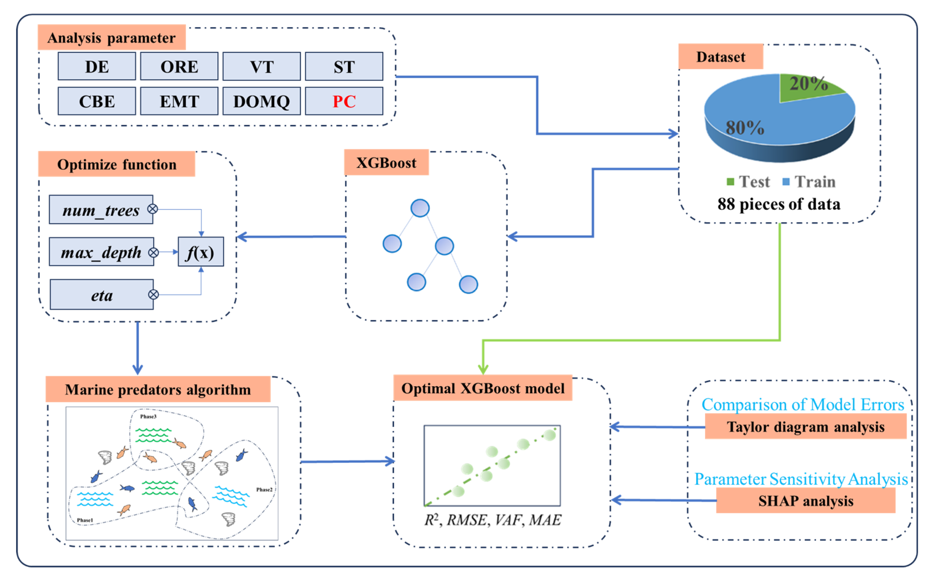
(1)

Collect data related to mining influencing factors and construct a dataset. Subsequently, randomly divide this dataset into a training subset (comprising 80% of the dataset) and a testing subset (constituting the remaining 20%). This random partitioning ensures that the model can generalize effectively to unseen data during the training phase.

(2)

Define an objective function aimed at optimizing the XGBoost parameters, focusing on num_trees, max_depth, and eta. In this study, the cross-validation score calculated across multiple optimization iterations serves as the evaluation metric for the objective function.

(3)

Employ the MPA to iteratively optimize parameter selection for XGBoost. During each iteration, evaluate the performance of each parameter set. Once the stopping criteria are satisfied, output the optimal parameters. Through this process, the best-fitting parameters for XGBoost are determined, enabling the construction of the coupled MPA–XGBoost model. This model is then utilized to establish a regression analysis framework linking PC with other mining-related influencing factors.

(4)

The performance of the MPA–XGBoost model is analyzed and compared with that of other machine learning models using the Taylor diagram methodology. Simultaneously, SHAP modeling is utilized to further elucidate the relationships and significance of various mining influencing factors on PC.

4. Results

4.1. Parameter Optimization Results

The swarm size of the optimization algorithm plays a critical role in determining the precision of the optimization process. Different particle swarm sizes lead to distinct optimization outcomes. Generally, a swarm size within the range of 20 to 100 is deemed appropriate. In this study, swarm sizes of 20, 40, 60, 80, and 100 were utilized, each with 120 iterations, to optimize the parameter selection for XGBoost via the MPA.

As depicted in Figure 6a, when the MPA is applied with varying swarm sizes, the fitness function achieves convergence after 90 iterations. It is worth highlighting that a swarm size of 60 results in the minimum fitness value (6.58 × 10⁻⁴). By evaluating the R², RMSE, VAF, and MAE scores using Equations (9) to (12) (Figure 6b–e), it can be observed that when the swarm size is 60, the five evaluation metrics collectively achieve optimal performance. Specifically, the R² score is 0.958, and the VAF is 95.981, both higher than those of other swarm sizes, indicating a superior fitting performance. Meanwhile, the MAE is 4.844, and the RMSE is 7.033, which are lower than those of other swarm sizes, suggesting minimal regression analysis error.

Table 2. Optimal calculation parameters.

Parameters	Value
num_trees	997
max_depth	8
eta	0.0650

presents the XGBoost parameters (num_trees, max_depth, and eta) obtained when the swarm size is 60. These parameters yield the most favorable regression analysis results, validating the optimal performance achieved with a swarm size of 60.

4.2. Comparison of the Accuracy of Regression Analysis Models

Based on the parameter optimization findings, an MPA–XGBoost model featuring a swarm size of 60 was selected for further analysis. The regression models concerning the PC and multi-factor indicators of the mining stope were evaluated using the test dataset. These models were subsequently compared with the outcomes derived from the standard XGBoost model, the PSO–XGBoost model, and the widely used regression-based machine learning method, SVM. As shown in Figure 7a–d, a comparative analysis of regression accuracy across different models is provided. The data points that are nearer to the function line (y = x) indicate smaller differences between the predicted and actual values, suggesting a higher level of model accuracy. Moreover, a greater concentration of data points within the ±20% error margin is indicative of superior model performance.

The MPA–XGBoost model demonstrates the most favorable evaluation metrics in the analysis of PC, as depicted in Figure 7a. Its R² value reaches 0.958, surpassing all other models, which clearly indicates a robust correlation between the predicted data and the actual data in the regression analysis. In addition, the VAF attains a high value of 95.981, ranking first among all regression methods, which vividly illustrates the remarkable explanatory power of the MPA–XGBoost model for the dataset. This results in highly reliable regression analysis outcomes. Moreover, both the MAE and RMSE values are minimized in the MPA–XGBoost model. Such minimization highlights the model’s outstanding ability to effectively capture the nonlinear patterns embedded within the PC dataset.

Compared with the traditional XGBoost prediction model, the MPA–XGBoost and PSO–XGBoost models demonstrate superior accuracy, as illustrated in Figure 7b,c. These findings highlight that incorporating population-based optimization algorithms enables more precise parameter tuning for XGBoost, leading to substantial improvements in the overall performance of the regression analysis model. Furthermore, the selection of optimization techniques plays a critical role in the parameter adjustment process within XGBoost. Notably, the MPA exhibits a better performance than the PSO algorithm during optimization. This is attributed to the tendency of the PSO algorithm to prematurely converge to local optima, whereas the MPA shows stronger global optimization capabilities.

When compared with conventional machine learning methods (as shown in Figure 7d), the MPA–XGBoost model demonstrates significant improvements in both regression analysis accuracy and associated error metrics. This model is capable of accurately capturing the complex relationships between PC and multiple influencing factors. Moreover, unlike traditional approaches, it optimizes the parameter selection process, thereby enhancing usability. In conclusion, when benchmarked against standard machine learning models, this approach achieves superior performance in terms of computational efficiency.

The Taylor diagram (Figure 7e) is developed based on the mean square deviation (SD), RMSE, and R² values of the four models [38]. The reference point REF, defined by a standard deviation (SD = 3), root mean square error (RMSE = 6), and coefficient of determination (R² = 1), established a rigorous and representative performance benchmark. This benchmark integrates critical dimensions such as data dispersion, prediction error, and goodness of fit, providing a robust quantitative foundation for objectively assessing the prediction accuracy of various models. Under this criterion, the distance between each model and REF directly indicates the precision of its predictions and evaluation metrics; shorter distances signify superior model performance. Through a systematic comparative analysis, the MPA–XGBoost model was identified as significantly outperforming other candidates, demonstrating a notably closer proximity to REF. This finding clearly underscores the model’s exceptional performance in terms of prediction accuracy and evaluation standards. Specifically, compared with traditional machine learning methods and other enhanced algorithms, the MPA–XGBoost model achieves a substantial advancement in regression analysis capabilities. It not only captures complex variable relationships with greater accuracy but also effectively minimizes prediction errors, thereby markedly improving the reliability and stability of its results.

4.3. SHAP Analysis Results

Prior analysis has demonstrated that the MPA–XGBoost model successfully establishes a comprehensive regression analysis framework by effectively identifying the relationships between various mining influence factors and PC. The model provides an accurate depiction of how different factors impact PC, highlighting the necessity for a deeper exploration of each factor’s contribution to PC. To achieve this, the SHAP method was employed to elucidate the importance and contribution of each feature to the PC outcomes, as illustrated in Figure 8.

To further and more comprehensively elucidate the contribution of each factor in the dataset to the research outcomes, we adopted a systematic analytical approach and conducted an in-depth examination of the overall impact and specific contributions of input factors on PC variations (for details, see Figure 8a,b). In these figures, the color coding serves as a clear indicator: colors closer to blue signify a stronger negative effect on PC, suggesting potential inhibition of or reduction in PC-related metrics; conversely, colors closer to red indicate a more pronounced positive influence on PC, likely enhancing or promoting its metrics. The parameters are arranged from top to bottom according to their overall influence in descending order, providing an intuitive visual comparison. Upon close observation and analysis, it becomes evident that among all the factors, DE exhibits the most significant overall influence. Specifically, DE contributes 35.6% to the total effect, underscoring its critical role and importance within the entire research framework.

When DE increases, the contribution points turn red, indicating a positive effect on PC; conversely, when DE decreases, the contribution points turn blue, indicating a negative effect. This suggests that DE has a significant positive influence on PC. VT, EMT, DOMQ, and ORE have similar contributions to PC, accounting for 14.2%, 13.9%, 13.7%, and 13.1% of the total impact, respectively. VT and EMT exhibit negative impacts on PC, while DOMQ and ORE show positive impacts. Other factors, such as ST and CBE, have relatively minor contributions to PC, accounting for 3.9% and 5.5%, respectively.

To further explore the specific influence patterns of different factors on PC, we selected the three most influential factors and constructed SHAP dependency plots (Figure 8c–e). These plots reveal that DE has a consistently positive impact on PC. Specifically, when DE exceeds 225 (the tipping point), PC shows a significant increase. VT and EMT both have negative impacts on PC. When VT and EMT are below the tipping point, PC decreases gradually; however, when they exceed the tipping point, PC drops sharply. The results suggest that enhancing the PC of the mining area can be achieved by increasing DE and reducing VT and EMT, leading to substantial improvements.

5. Discussions

This study analyzed the weak links of the mechanized mining system in underground metal mines using machine learning and SHAP interpretable models. The research findings hold theoretical and practical significance in multiple aspects but also have certain limitations. Numerous expandable research directions remain for future exploration.

From the perspective of model construction and optimization, the MPA–XGBoost coupling model demonstrates superior performance. By optimizing the parameters of the XGBoost model using the MPA, the regression analysis achieves excellent goodness of fit and error control. Compared with traditional XGBoost models and other machine learning techniques such as SVM, the MPA–XGBoost model exhibits higher R² values, lower RMSE and MAE, and is closer to the reference point in the Taylor diagram. This indicates its enhanced ability to accurately capture the complex nonlinear relationships between the production capacity of the mining area (PC) and various influencing factors. However, the model’s performance is contingent on the selected dataset. The data used in this study were derived from a decade of mining operations at Tongkeng Mine, which introduces regional and temporal limitations. Different mines exhibit significant variations in geological conditions, mining processes, and equipment levels [39]. Future research should broaden the data collection scope to include more diverse mine data, thereby further validating and optimizing the model and enhancing its generalizability.

In terms of the analysis of influencing factors, the SHAP method elucidates the contribution and impact patterns of each factor on PC. DE demonstrates the most significant positive influence on PC, whereas VT and EMT exhibit notable negative impacts. This insight provides clear guidance for mine production management, enabling mines to implement targeted measures. For instance, mines can optimize the selection and operation of rock drilling equipment to enhance DE, design efficient ventilation systems to reduce VT, and formulate scientific maintenance plans to minimize EMT, thereby improving overall production efficiency.

From the perspective of practical applications, the research findings can directly support the refined management of mines. Based on these conclusions, mines can optimize their mining processes by adopting efficient equipment and enhancing drilling techniques during the rock drilling stage; strategically arranging ventilation facilities to achieve rapid ventilation during the ventilation stage; and establishing an intelligent monitoring system during the equipment maintenance stage to predict equipment failures and conduct proactive maintenance, thereby reducing downtime. However, during the actual promotion and application process, several challenges may arise, such as high technical costs and personnel qualifications. Introducing new equipment and technologies requires substantial capital investment, which some mines may find difficult to afford. Additionally, the adoption of new technologies demands higher professional skills from employees, necessitating enhanced training programs to improve their operational and management capabilities, ensuring that the research findings can be effectively implemented [40].

Future research can further broaden the scope of data samples to encompass mines with diverse geological conditions and mining processes, thereby enhancing the generalizability of the research outcomes. Additionally, future studies can delve deeper into the complex interactions among various factors to provide more comprehensive and precise decision support for optimizing mining systems [41]. With the advancement of intelligent mine construction, future research can integrate cutting-edge technologies such as the Internet of Things (IoT), big data, and artificial intelligence (AI) [42,43,44]. By leveraging the IoT for real-time data collection and transmission, a larger and more dynamic dataset can be constructed, which will further improve the accuracy of model predictions and enhance the understanding of complex systems [45]. This integration will promote the development of underground metal mining towards greater intelligence, efficiency, and safety.

6. Conclusions

This study comprehensively utilized machine learning and SHAP interpretability models to systematically analyze the weak links in the mechanized mining system of underground metal mines, leading to the following key conclusions:

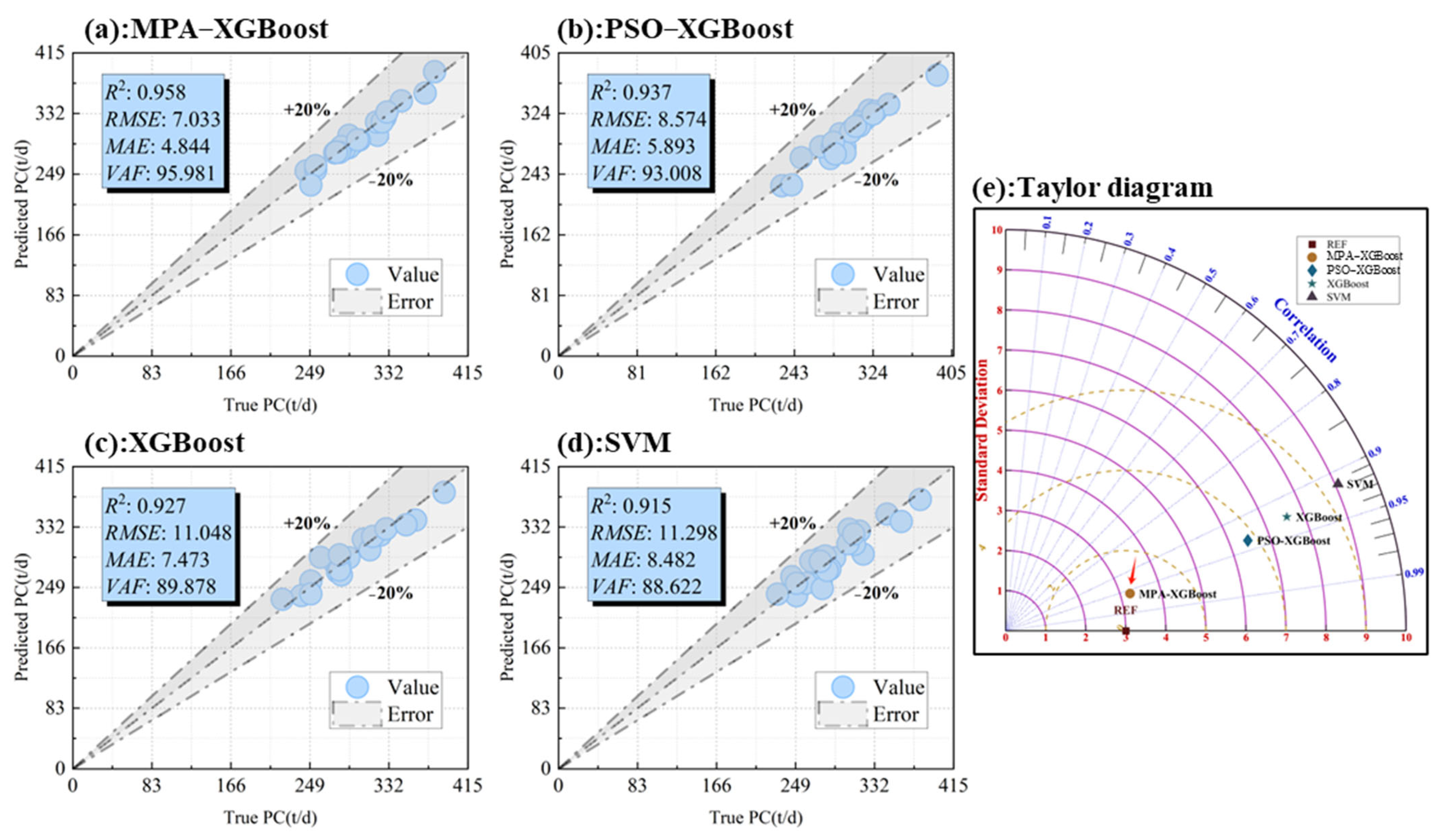
(1)

The XGBoost algorithm was employed to establish a regression relationship between multiple factors and the production capacity of the stope (PC), with parameters optimized using the MPA. The results demonstrated that the MPA achieved an optimal performance with a swarm size of 60. Under these conditions, the MPA–XGBoost coupling model exhibited an exceptional predictive performance for PC, achieving an R² value of 0.958, VAF of 95.981%, MAE of 4.844, and RMSE of 7.033. Compared with traditional XGBoost models, PSO–XGBoost models, and common machine learning techniques such as SVM, this model showed significant advantages in regression accuracy, dataset interpretability, and capturing nonlinear relationships, providing a more precise representation of the relationship between PC and various influencing factors.

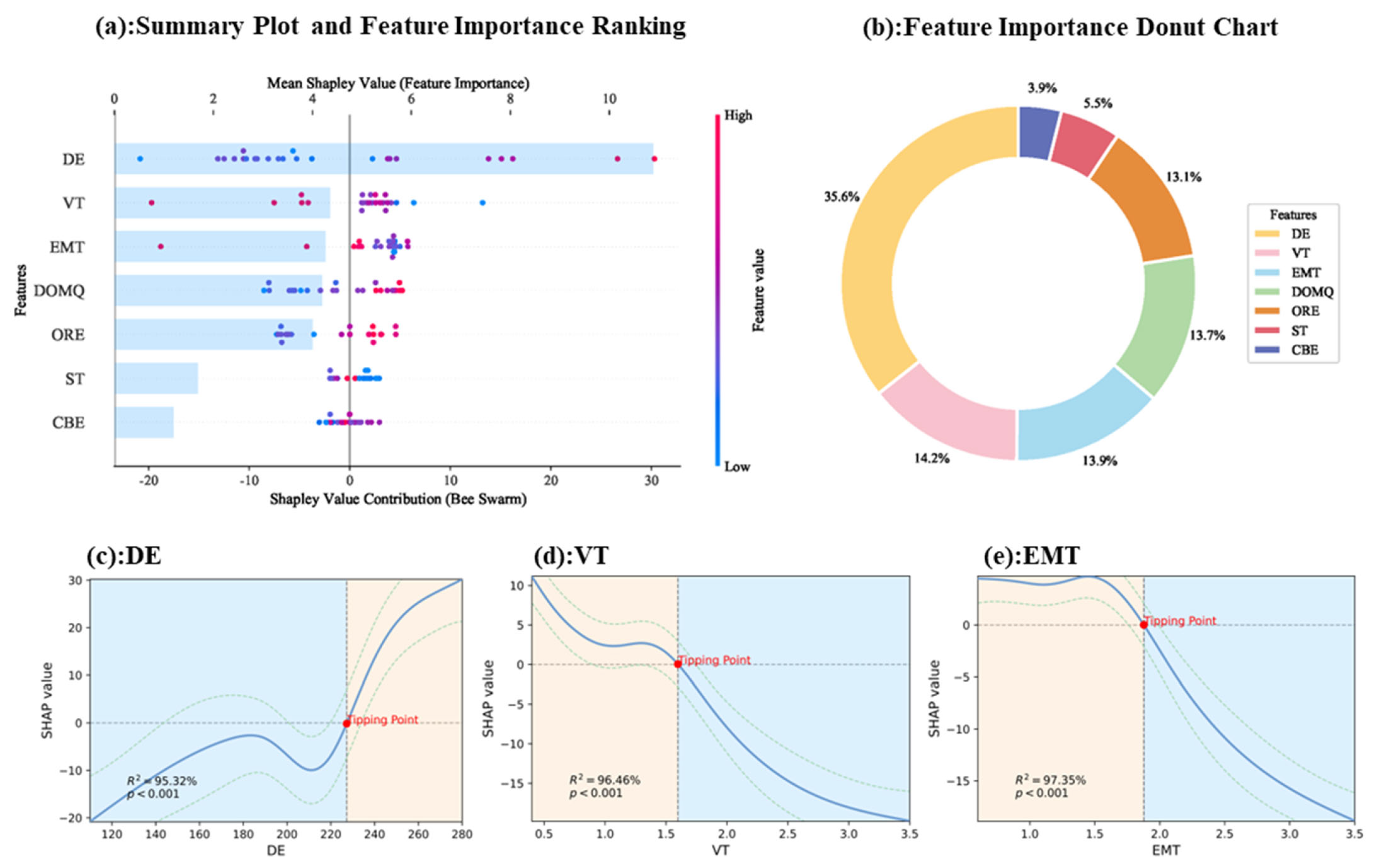
(2)

Using the SHAP method, the importance and contribution degree of different stope mining factors to PC were quantified. DE had the most significant overall impact on PC, contributing positively by 35.6%. VT, EMT, DOMQ, and ORE had similar contributions, accounting for 14.2%, 13.9%, 13.7%, and 13.1%, respectively. Among these, VT and EMT exerted negative impacts, while DOMQ and ORE had positive effects. ST and CBE had relatively smaller contributions, at 3.9% and 5.5%, respectively.

(3)

By constructing SHAP dependency plots, the influence patterns of key factors on PC were clearly illustrated. As DE increased, PC significantly improved, particularly when DE exceeded 225, where the effect became more pronounced. For VT and EMT, PC decreased gradually below a specific threshold (the tipping point) but dropped sharply above it. This indicates that increasing DE and reducing VT and EMT can significantly enhance stope PC.

(4)

This study effectively identified the weak links in the mechanized mining system of underground metal mines through advanced modeling, quantified the impact of various factors on mining efficiency, and provided a scientific basis for optimizing mining processes. Mining production managers can leverage these findings to improve specific production processes, such as enhancing drilling efficiency, optimizing ventilation systems, and refining equipment maintenance procedures, thereby boosting overall mine productivity and ensuring safe operations.

References

- Boloz, L.; Bialy, W. Automation and Robotization of Underground Mining in Poland. Appl. Sci. 2020, 10, 7221. [Google Scholar] [CrossRef]
- Eddies, R.; Wood, R.; Haynes, A.; Warburton, D.; Pressdee, C. Screening ground risk in underground works as part of a predictive modelling approach. Proc. Inst. Civ. Eng. Civ. Eng. 2020, 173, 49–57. [Google Scholar] [CrossRef]
- Fang, J.; Fan, C.; Wang, F.R.; Bai, D.X. Augmented Reality Platform for the Unmanned Mining Process in Underground Mines. Min. Metall. Explor. 2022, 39, 385–395. [Google Scholar] [CrossRef]
- Gao, R.G.; Zhou, K.P.; Yang, C.; Zhu, K. An Underground Mine Risk Identification Model and Safety Management Method Based on Explanation Graph-Probabilistic Multi-Plan Analysis (EG-PMPA). IEEE Access 2020, 8, 223214–223233. [Google Scholar] [CrossRef]
- Ghorbani, Y.; Nwaila, G.T.; Zhang, S.E.; Bourdeau, J.E.; Cánovas, M.; Arzua, J.; Nikadat, N. Moving towards deep underground mineral resources: Drivers, challenges and potential solutions. Resour. Policy 2023, 80, 103222. [Google Scholar] [CrossRef]
- Gligoric, Z.; Beljic, C.; Gluscevic, B.; Cvijovic, C. Underground Lead-Zinc Mine Production Planning Using Fuzzy Stochastic Inventory Policy. Arch. Min. Sci. 2015, 60, 73–92. [Google Scholar] [CrossRef]
- Hou, J.; Li, G.Q.; Chen, L.Y.; Wang, H.; Hu, N.L. Optimization of Truck-Loader Matching Based on a Simulation Method for Underground Mines. Sustainability 2023, 15, 216. [Google Scholar] [CrossRef]
- Iphar, M.; Alpay, S. A mobile application based on multi-criteria decision-making methods for underground mining method selection. Int. J. Min. Reclam. Environ. 2019, 33, 480–504. [Google Scholar] [CrossRef]
- Laptev, V.V.; Gurin, K.P. Automated Planning of Underground Mining Operations with Regard to Geological and Geotechnical Constraints. J. Min. Sci. 2023, 59, 490–496. [Google Scholar] [CrossRef]
- Lu, G.Z.; Wang, R.; Li, Q.S.; Hu, F. Three-Dimensional Dynamic Visualization Simulation of Underground Mining Engineering considering Chaos Optimization of Symmetric Varieties. Mob. Inf. Syst. 2022, 2022, 2916971. [Google Scholar] [CrossRef]
- Onifade, M.; Said, K.O.; Shivute, A.P. Safe mining operations through technological advancement. Process Saf. Environ. Prot. 2023, 175, 251–258. [Google Scholar] [CrossRef]
- Villalba Matamoros, M.E.; Kumral, M. A value adding approach to hard-rock underground mining operations: Balancing orebody orientation and mining direction through meta-heuristic optimization. J. Cent. South Univ. 2019, 26, 3126–3139. [Google Scholar] [CrossRef]
- Vogt, D. A review of rock cutting for underground mining: Past, present, and future. J. S. Afr. Inst. Min. Metall. 2016, 116, 1011–1026. [Google Scholar] [CrossRef]
- Vogt, D.; Hattingh, T. The importance of people in the process of converting a narrow tabular hard-rock mine to mechanization. J. S. Afr. Inst. Min. Metall. 2016, 116, 265–274. [Google Scholar] [CrossRef]
- Yang, C.T.; Zhang, R.P.; Liu, D.W.; Tang, Y.; Huang, R.D.; Qiu, W.C. Evaluation of Excavation Ergonomics of Drill and Blast Method Based on Game Theory G2-EW-TOPSIS Model. Appl. Sci. 2023, 13, 7205. [Google Scholar] [CrossRef]
- Wang, S.F.; Wu, Y.M.; Shi, X.L. Non-explosive mechanized and intelligent mining/heading in underground mine. Trans. Nonferrous Met. Soc. China 2024, 34, 265–282. [Google Scholar] [CrossRef]
- Nehring, M.; Topal, E.; Little, J. A new mathematical programming model for production schedule optimization in underground mining operations. J. S. Afr. Inst. Min. Metall. 2010, 110, 437–446. [Google Scholar]
- Sotoudeh, F.; Nehring, M.; Kizil, M.; Knights, P.; Mousavi, A. Production scheduling optimisation for sublevel stoping mines using mathematical programming: A review of literature and future directions. Resour. Policy 2020, 68, 101809. [Google Scholar] [CrossRef]
- Appianing, E.J.A.; Ben-Awuah, E.; Pourrahimian, Y. Life-of-mine optimization for integrated open stope development and production scheduling using a mixed-integer linear programming framework. Min. Technol. Trans. Inst. Min. Metall. 2023, 132, 106–120. [Google Scholar] [CrossRef]
- Huang, S.W.; Li, G.Q.; Ben-Awuah, E.; Afum, B.O.; Hu, N.L. A Stochastic Mixed Integer Programming Framework for Underground Mining Production Scheduling Optimization Considering Grade Uncertainty. IEEE Access 2020, 8, 24495–24505. [Google Scholar] [CrossRef]
- Liu, D.; Li, G.Q.; Hu, N.L.; Xiu, G.L.; Ma, Z.Y. Optimization of the cut-off grade for underground polymetallic mines. Gospod. Surowcami Miner. Miner. Resour. Manag. 2019, 35, 25–42. [Google Scholar] [CrossRef]
- Ali, D.; Frimpong, S. Artificial intelligence, machine learning and process automation: Existing knowledge frontier and way forward for mining sector. Artif. Intell. Rev. 2020, 53, 6025–6042. [Google Scholar] [CrossRef]
- Chimunhu, P.; Topal, E.; Ajak, A.D.; Asad, W. A review of machine learning applications for underground mine planning and scheduling. Resour. Policy 2022, 77, 102693. [Google Scholar] [CrossRef]
- Patil, S.D.; Mitra, A.; Katarikonda, K.T.; Wansink, J.D. Predictive asset availability optimization for underground trucks and loaders in the mining industry. Opsearch 2021, 58, 751–772. [Google Scholar] [CrossRef]
- Taboada, J.; Matías, J.M.; Araújo, A.; Ordóñez, C. Assessing the viability of underground slate mining by combining an expert system with a GIS. Eng. Geol. 2006, 87, 75–84. [Google Scholar] [CrossRef]
- Witulska, J.; Stefaniak, P.; Jachnik, B.; Skoczylas, A.; Sliwinski, P.; Dudzik, M. Recognition of LHD Position and Maneuvers in Underground Mining Excavations-Identification and Parametrization of Turns. Appl. Sci. 2021, 11, 6075. [Google Scholar] [CrossRef]
- Gao, F.; Li, X.; Xiong, X.; Lu, H.C.; Luo, Z.W. Refined Design and Optimization of Underground Medium and Long Hole Blasting Parameters-A Case Study of the Gaofeng Mine. Mathematics 2023, 11, 1612. [Google Scholar] [CrossRef]
- Tu, S.Y.; Jia, M.T.; Wang, L.G.; Feng, S.Z.; Huang, S. A Dynamic Scheduling Model for Underground Metal Mines under Equipment Failure Conditions. Sustainability 2023, 15, 7306. [Google Scholar] [CrossRef]
- Yu, Z.; Li, C.Q.; Zhou, J. Tunnel Boring Machine Performance Prediction Using Supervised Learning Method and Swarm Intelligence Algorithm. Mathematics 2023, 11, 4237. [Google Scholar] [CrossRef]
- Zhou, J.; Qiu, Y.G.; Zhu, S.L.; Armaghani, D.J.; Khandelwal, M.; Mohamad, E.T. Estimation of the TBM advance rate under hard rock conditions using XGBoost and Bayesian optimization. Undergr. Space 2021, 6, 506–515. [Google Scholar] [CrossRef]
- Hong, Z.X.; Tao, M.; Liu, L.L.; Zhao, M.S.; Wu, C.Q. An intelligent approach for predicting overbreak in underground blasting operation based on an optimized XGBoost model. Eng. Appl. Artif. Intell. 2023, 126, 107097. [Google Scholar] [CrossRef]
- Al-Betar, M.A.; Awadallah, M.A.; Makhadmeh, S.N.; Alyasseri, Z.A.A.; Al-Naymat, G.; Mirjalili, S. Marine Predators Algorithm: A Review. Arch. Comput. Methods Eng. 2023, 30, 3405–3435. [Google Scholar] [CrossRef] [PubMed]
- Faramarzi, A.; Heidarinejad, M.; Mirjalili, S.; Gandomi, A.H. Marine Predators Algorithm: A Nature-inspired Metaheuristic. Expert Syst. Appl. 2020, 152, 113377. [Google Scholar] [CrossRef]
- Mugemanyi, S.; Qu, Z.Y.; Rugema, F.X.; Dong, Y.C.; Wang, L.; Bananeza, C.; Nshimiyimana, A.; Mutabazi, E. Marine predators algorithm: A comprehensive review. Mach. Learn. Appl. 2023, 12, 100471. [Google Scholar] [CrossRef]
- Guo, H.; Lin, L.; Wu, J.L.; Lv, Y.C.; Tong, C.S. Optimizing Driving Parameters of the Jumbo Drill Efficiently with XGBoost-DRWIACO Framework: Applied to Increase the Feed Speed. Sensors 2024, 24, 2600. [Google Scholar] [CrossRef]
- Tao, M.; Zhao, Q.Z.; Zhao, R.; Burhan, M.M. A New Method of Rockburst Prediction for Categories with Sparse Data Using Improved XGBoost Algorithm. Nat. Resour. Res. 2025, 34, 599–618. [Google Scholar] [CrossRef]
- Xu, C.; Zhou, K.P.; Xiong, X.; Gao, F.; Lu, Y. Prediction of mining induced subsidence by sparrow search algorithm with extreme gradient boosting and TOPSIS method. Acta Geotech. 2023, 18, 4993–5009. [Google Scholar] [CrossRef]
- He, Z.G.; Armaghani, D.J.; Masoumnezhad, M.; Khandelwal, M.; Zhou, J.; Murlidhar, B.R. A Combination of Expert-Based System and Advanced Decision-Tree Algorithms to Predict Air-Overpressure Resulting from Quarry Blasting. Nat. Resour. Res. 2021, 30, 1889–1903. [Google Scholar] [CrossRef]
- Zhao, Y.F.; Chen, J.H.; Yang, S.; Chen, Y. Mining Plan Optimization of Multi-Metal Underground Mine Based on Adaptive Hybrid Mutation PSO Algorithm. Mathematics 2022, 10, 2418. [Google Scholar] [CrossRef]
- Wang, H.; Zhang, X.X.; Yuan, H.; Wu, Z.G.; Zhou, M. A Lean Scheduling Framework for Underground Mines Based on Short Interval Control. Sustainability 2023, 15, 9195. [Google Scholar] [CrossRef]
- Sari, Y.A.; Kumral, M. Clustering-based iterative approach to stope layout optimization for sublevel stoping. J. South. Afr. Inst. Min. Metall. 2021, 121, 97–106. [Google Scholar] [CrossRef]
- Fulawka, K.; Szumny, M.; Mertuszka, P. Rock Mass Preconditioning Methods in Underground Mines and Ways of Its Evaluation-State-of-the-Art. Civ. Environ. Eng. Rep. 2024, 34, 381–402. [Google Scholar] [CrossRef]
- Hou, J.; Li, G.Q.; Wang, H.; Hu, N.L. Genetic algorithm to simultaneously optimise stope sequencing and equipment dispatching in underground short-term mine planning under time uncertainty. Int. J. Min. Reclam. Environ. 2020, 34, 307–325. [Google Scholar] [CrossRef]
- Pääkkönen, P.; Horsmanheimo, S.; Pakkala, D.; Tuomimäki, L.; Backman, J. Reference architecture design and evaluation for digitalization of underground mining. Internet Things 2024, 26, 101238. [Google Scholar] [CrossRef]
- Salinas, J.P.; Araujo, J.J.M.; Teatino, M.A.C. Uncertainty in underground mining operations: A bibliometric and systematic literature review analysis. World J. Eng. 2024. [Google Scholar] [CrossRef]