Abstract
This paper presents a study on the optimization of 2,4-Dichlorophenoxyacetic (2,4-D) acid removal from synthetic wastewater by batch Fenton-Ozonation. The aim of this study is to evaluate the potential of the catalytic system Fe-L27 coupled to ozonation in the presence and absence of H2O2 as an effective and affordable technique for the treatment of organic pollutants in water. Fenton-like catalysts for the removal of 2,4-D in aqueous solutions were elaborated using catalysts synthesized by the wet impregnation method. The ACs and prepared catalysts were characterized by nitrogen adsorption–desorption isotherms at 77 K, TGA, XPS, SEM, and TEM. Their efficiency as Fenton-like catalysts was studied. In a first step, a response surface modeling method was employed in order to find the optimal parameters of the Fenton process, and then the optimal O3/H2O2 ratio was established at laboratory scale. Finally, the investigated advanced oxidation processes were carried out at pilot scale. The results show that Fenton-like catalysts obtained by the direct impregnation method enhance the degradation rate and mineralization of 2,4-D.
1. Introduction
Activated carbons (ACs) have been widely used for many years as adsorbent materials for gas and liquid separation and purification. For each of these applications and the associated chemical species to be separated or purified, a suitable material is required. This is particularly true when treating natural aqueous matrices such as polluted water [1,2]. In order to treat the latter, it is necessary to have a material with an optimum porous texture for which the performance of the adsorption process will be maximized for a given type of molecule, while considering other influencing factors such as surface chemistry and environmental conditions [3,4,5]. In addition to their use in liquid-phase adsorption processes, ACs can be integrated into advanced oxidation processes by acting as pseudo-catalysts for hydroxyl radicals [6,7,8,9,10]. Hydroxyl radicals are powerful oxidizers of organic compounds. As a result, they can lead to their total mineralization in the form of carbon dioxide. While these hydroxyl radicals can be generated by ozone reacting with activated carbon in the presence of hydrogen peroxide (known as the peroxone system), they canalso be generated by hydrogen peroxide reacting with metals such as iron (in the Fe2+ form), and in particular its oxide (known as the Fenton system) [11,12,13]. However, the efficiency of mineralization strongly depends on the operational conditions specific to the applied oxidation process. In this context, Kamenická and Weidlich (2023) compared various oxidative and reductive approaches for the treatment of mordant blue 9, a chlorinated azo dye, and highlighted the critical influence of reagent selection and the molecular properties of the pollutant on the overall performance of the process [13]. Nevertheless, coupling these two reaction systems, peroxone and Fenton, should enable optimum mineralization of certain organic pollutants in the aqueous phase. Within the framework of these advanced oxidation processes (AOPs) couplings, it is important to identify the most efficient carbonaceous material for these specific applications for the degradation and mineralization of persistent organic molecules present in water, and to optimize the experimental parameters of these processes.
This study focuses on 2,4-dichlorophenoxyacetic (2,4-D), a widely used herbicide in agriculture and gardening to control broad-leaved weeds [14,15]. Its use is favored due to its low cost and effectiveness in controlling weeds in corn, coffee, and soybean crops [14,15]. Although its use in France, for example, has been steadily decreasing since 2011 (674 tons of 2,4-D sold in 2011 compared to 350 tons in 2019), this product can still be considered relatively commonly used [16]. 2,4-D is a low-dissociation phenoxy-acid herbicide characterized by an electron density of π on its phenyl ring. However, its low pKa of 2.8 indicates that it is predominantly anionic (2,4-dichlorophenoxyacetate) at pH above 2.8, while it takes a neutral form below this value. The environmental problem linked to the use of this product is that its presence in the environment increases the risk of soil and aquatic pollution (surface water and groundwater). This pollution is the result of the transfer of these products from the soil to the water via the phenomena of bursting and infiltration into the soil. 2,4-D, being highly soluble in water (900 mg·L−1) [17,18], is easily transported in aquatic environments and in the soil. In addition, since 2015, 2,4-D has been classified as a probable carcinogen for humans (carcinogenic group 2B) by the International Agency for Research on Cancer (IARC) and the World Health Organization (WHO) [19]. However, the use of this herbicide is still allowed in the European Union. This highlights the importance of removing this pollutant from water.
This molecule is chosen for its resistance to degradation by conventional processes (such as chlorination or biological processes) and its relative ease of analysis, making it an ideal target for assessing the effectiveness of AOPs on these materials. Various studies have shown various methods of processing 2,4-D, including adsorption on activated carbon [5,16,20], microbial degradation [21], electrochemical oxidation [22], photocatalytic oxidation [18], and non-thermal plasma oxidation [16].
This study focuses on the degradation and mineralization of 2,4-D by the Fenton process, which relies on the reaction between hydrogen peroxide (H2O2) and ferrous ions (Fe2+) to generate highly reactive hydroxyl radicals capable of breaking down pollutants. This work shows that it is possible to optimize and evaluate the performance of each process, not only in terms of pollutant concentration reduction, but also in terms of mineralization, i.e., the complete conversion of organic molecules into inorganic products such as water and carbon dioxide. For this, iron-enriched carbon materials are synthesized for use as catalyst carriers in the Fenton process. An experimental design was employed to determine the optimal conditions for degradation and mineralization of pollutants in water. Modeling and optimization of the 2,4-dichlorophenoxyacetic degradation process were performed by means of a central composite design (CCD). Its characterization is performed by dinitrogen adsorption at 77 K, thermogravimetric analysis (TGA), and scanning electron microscopy (SEM).
2. Materials and Methods
2.1. Materials
Ferrous sulphate heptahydrate (FeSO4 × 7H2O, Sigma Aldrich, Saint Louis, MO, USA, 99%), hydrogen peroxide (H2O2, Sigma Aldrich, 35%), 2,4-dichlorophenoxyacetic (2,4-D, Sigma Aldrich, ≥97%), thiosulfate of sodium (Na2S2O3, Sigma Aldrich, 99%), and activated carbon L27, provided by Jacobi Carbons, were used for this study. For the development of iron-enriched ACs, a commercial AC (L27) and a protocol developed by Secula et al. [23] were used. The latter was washed beforehand to remove acid residues from the industrial process of producing L27. For this, a weight of 15 g of ACs was stirred in 2 L of distilled water for 24 h and then rinsed several times until a neutral pH (6.5) filtrate was obtained. Iron grafting was performed from an iron sulphate solution prepared by dissolving 12.641 g of FeSO4.7H2O in 100 mL of ultra-pure water, thus obtaining a concentration of 25.4 g L−1 of Fe. Then, a weight of 10 g of washed AC was soaked with 100 mL of this solution under stirring in a water bath at 55 °C until the water evaporated completely. The objective was to obtain a material containing 80% AC and 20% iron. After filtration, the AC-Fe was dried at 80 °C for 12 h. A second wash step was carried out to remove the unfixed iron and impurities, followed by an additional drying at 80 °C. Finally, a heat treatment under a nitrogen atmosphere fixed the iron on the material and removed residual impurities and sulphates. The AC-Fe was heated in a tubular oven under a flow of nitrogen (160 mL min−1) with a temperature rise of 20 °C min−1 from ambient temperature to 800 °C, maintained for 1 h, and then cooled down to room temperature.
2.2. Characterization Methods
The thermal degradation profile of the AC was obtained by thermogravimetric analysis (STA 449 F5 Jupiter-NETZSCH, NETZSCH, Selb, Germany). A sample of approximately 0.04 g was analyzed in a thermobalance under a 160 mL/min argon flow. A blank experiment was conducted under identical conditions for baseline correction. The procedure involved heating from room temperature to 800 °C at 5 °C/min, maintaining the temperature for 1 h, and then cooling to room temperature. Textural properties (surface area, pore volume, and mean pore size) were determined using dinitrogen adsorption isotherms at 77 K (Micromeritics ASAP 2020, Micromeritics Instrument Corporation, Norcross, GA, USA). Beforehand, the samples were degassed at 250 °C for at least 24 h under a residual vacuum of at least 6 μmH. Textural properties (i.e., specific surface area, pore size distributions, average micropore sizes, etc.) of the ACs were obtained using a routine based on the 2D-NLDFT model (N2 at 77 K for heterogenous surface carbons), which is implemented in the SAIEUS software (version 3.0) [24]. The surface chemical functionalities were analyzed by FTIR (Thermo Scientific Nicolet IS50 FT-IR, Thermo Fisher Scientific, Waltham, MA, USA) in transmission mode and by XPS. The XPS analyses were carried out using a Thermo Scientific Escalab Xi+ spectrometer operating at 10−10 mbar in continuous energy scan mode at 200 eV, with a spot size of 650 μm, and equipped with a non-monochromatic X-ray source producing Al Kα or Ag Lα photons with energies of 1486.6 eV or 3000 eV. The samples were exposed to monochromatic Al Kα X-ray photons (hv = 1486.6 eV). The C1s carbon peak was at 284.5 eV and was used to calibrate the binding energies. Peak deconvolution was performed using Thermo Scientific Avantage software (Version 5.0). Finally, the morphology of the AC was determined from scanning electron microscopy (SEM) and transmission electron microscopy (TEM, JEOL-IT800SHL, JEOL Ltd., Tokyo, Japan) analyses.
2.3. Fenton Process Tests
The Fenton process was carried out according to a spherical central composite experimental design. A 200 mL volume of a 100 mg·L−1 solution of 2,4-D was brought into contact in a 250 mL reactor. Factor 1 is for the AC dose (mg·L−1), factor 2 for H2O2 dose (mg·L−1), and factor 3 for pH variation. These parameters were considered in order to determine the optimal parameters for the Fenton process. To monitor degradation kinetics, samples of the solution were taken between 1 min and 60 min. Thus, a 2 mL volume of the treated solution was taken, filtered, and then diluted in an 18 mL volume of sodium sulphite (1 mol·L−1) to stop the degradation reactions.
2.4. Ozonation Process Tests
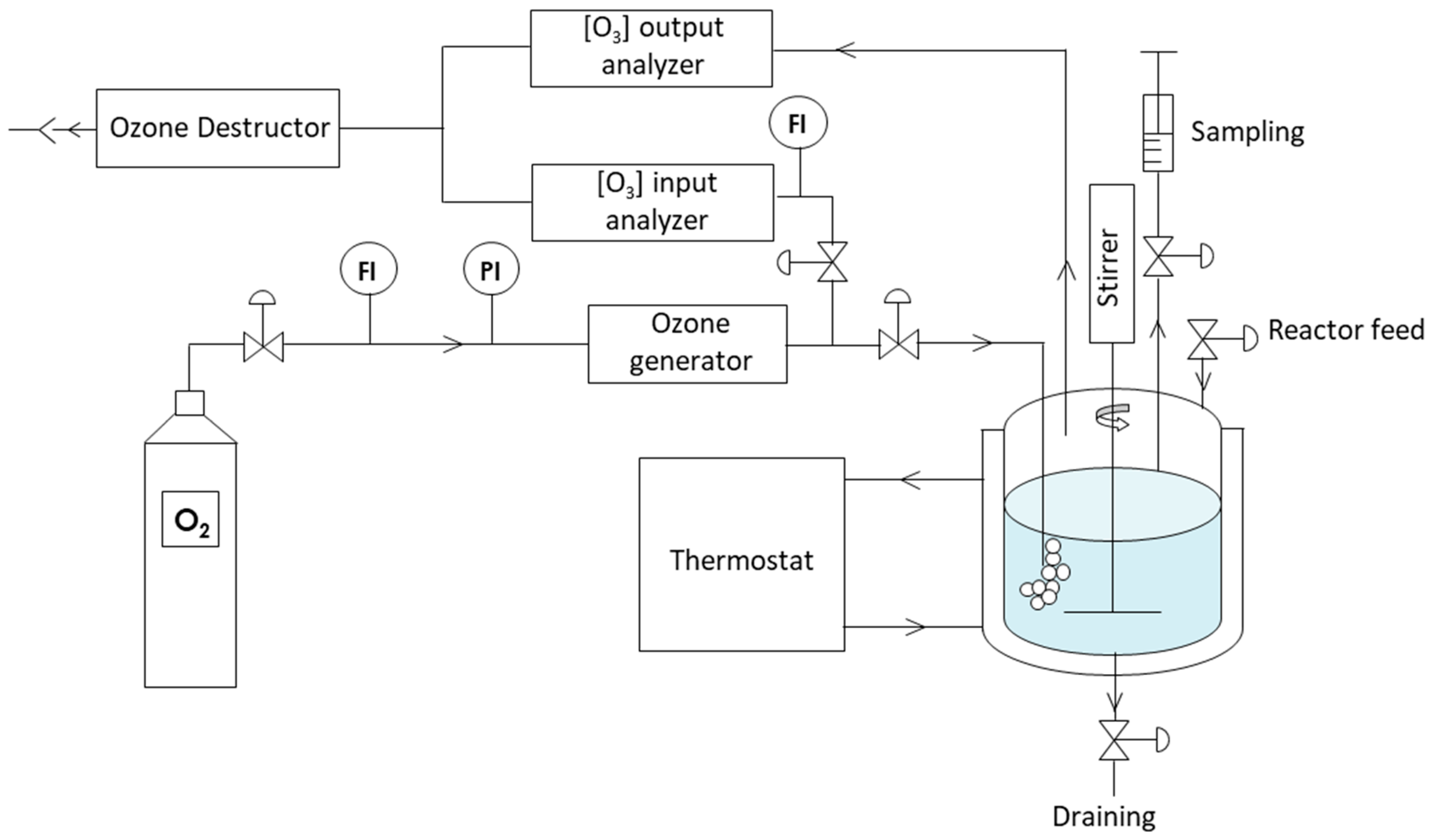
The ozonation process was carried out in a double-jacketed glass reactor (1 L) equipped with a stirring system (a 30 cm impeller) and a sampling device. Figure 1 presents the ozonation laboratory set-up (described in [25]). The temperature was maintained at 25 °C by a thermostatic fluid circulating in the double jacket. The gas circuit materials (PTFE tubing and PFA valves) were used to prevent any interaction with ozone. Ozone was produced by electrical discharge in a flow of pure oxygen (40 NL·h−1), with its flow rate and pressure controlled by a flow meter and a pressure gauge. Ozone production was adjusted via a potentiometer, and its voltage was monitored by a voltmeter. The ozonated gas was directed into the reactor through a porous diffuser, and part of the flow was analyzed using a UV system at 254 nm to evaluate the ozone concentration, with protection provided by a washing flask. Finally, any unreacted ozone was eliminated from the reactor through a catalytic destructor before discharge into the atmosphere, ensuring an outlet ozone concentration close to zero. The ozonation process was realized with 500 mL of solution, containing 100 mg·L−1 of organic pollutant. The ozone concentration of 25 g Nm−3 was adjusted using an ozone generator. The choice of these parameters was based on the work of Ferreira de Oliveira and those of Samba [25,26].
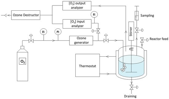
Figure 1.
Ozonation pilot experimental set-up.
2.5. Analysis Methods
Kinetic monitoring of the concentration of the solution to be treated was carried out using HPLC (DAD detection), along with monitoring of changes in total organic carbon (TOC) over time. The HPLC method was validated in terms of linearity, sensitivity, and precision. Calibration was performed using at least five concentration levels of 2,4-dichlorophenoxyacetic acid (2,4-D) (Sigma-Aldrich, ≥97%). The limit of detection (LOD) and limit of quantification (LOQ) were determined following ICH guidelines, using the standard deviation of the response and the slope of the calibration curve [27]. The resulting values were 0.24 mg·L−1 (LOD) and 0.72 mg·L−1 (LOQ). TOC measurements were validated in a similar manner. Calibration was performed using standard TOC solutions from Sigma Aldrich. The LOD and LOQ for TOC were calculated analogously to the HPLC method and were determined to be 0.63 mg·L−1 and 1.90 mg·L−1, respectively.
HPLC analysis was used to evaluate the degradation (abatement) of 2,4-D during the oxidation, while TOC measurements were used to monitor the mineralization of the molecule as the treatment progressed. Operating conditions for the HPLC analyses are provided in Table 1.

Table 1.
HPLC operating conditions.
The efficiency of the processes to eliminate 2,4-D was determined from the degradation rate (YHPLC), which represents the removal efficiency of the concentration of the pollutant in the solution, and the mineralization rate (YTOC), which gives the mineralization efficiency (transformation into CO2 and H2O) of 2,4-D. These parameters are given by the following equations, in which TOC0 et TOCt are the concentrations of total organic carbon (mg L−1) at time t and at t = 0, and C0 and Ct are the concentrations of the solutions (mg L−1) at time t and at t = 0 (determined by HPLC).
The modeling of the degradation kinetics of 2,4-D was carried out according to the pseudo-first-order model. For the case of ozonation, the concentration of ozone and hydroxyl radicals was considered constant. In this case, the degradation was dependent on the concentration of 2,4-D in the solution [28,29] and is given by the following equation:
In this equation, C represents the pollutant concentration in mg L−1 and Kapp is the apparent degradation rate constant, expressed in min−1. Integration of the rate law between t = 0 and any time t, where the pollutant concentrations are C0 and Ct, respectively, leads to the following expression, in which kapp corresponds to the slope of the variation linear plot of ln(Ct/C0) versus time.
2.6. Experimental Design
A spherical central composite experimental design (CCD) for three factors was generated to optimize by RSM the Fenton degradation of a model pollutant using Design Expert software (State-Ease Inc., Minneapolis, MN, USA, Version 7.1.5). The solution pH and catalyst doses (L27-Fe and H2O2) were chosen as independent variables. This kind of CCD allows one to consider a wider range for each considered factor.
The operating ranges of the three factors of the Fenton process are shown in Table 2.
Table 2.
Predictor variables and actual values (zi) used in the experimental design (α = 1.73205).
3. Results
A spherical central composite experimental design composed of 15 runs and 3 replicates (Table 2) was used for response surface modeling. The experimental data were analyzed by the Multi Linear Regression (MLR—regression model with the lowest residual sum of squares of the response) method to fit the second-order polynomial equation:
where β0, βi, βii, and βij are regression coefficients (β0 is a constant term, βi is a liner effect term, βii is a squared effect term, and βij is an interaction effect term), and Y is the predicted response value.
As response for modeling, 2,4-D removal efficiency in relation to HPLC and TOC data were considered.
The experimental results listed in Table 3 and Table A1 were determined according to the planned initial conditions.
Table 3.
Spherical (α =1.73205)—CCD experimental design and the predicted and observed values of responses: YTOC 10–60 min and YHPLC 60 min.
3.1. Fenton Process
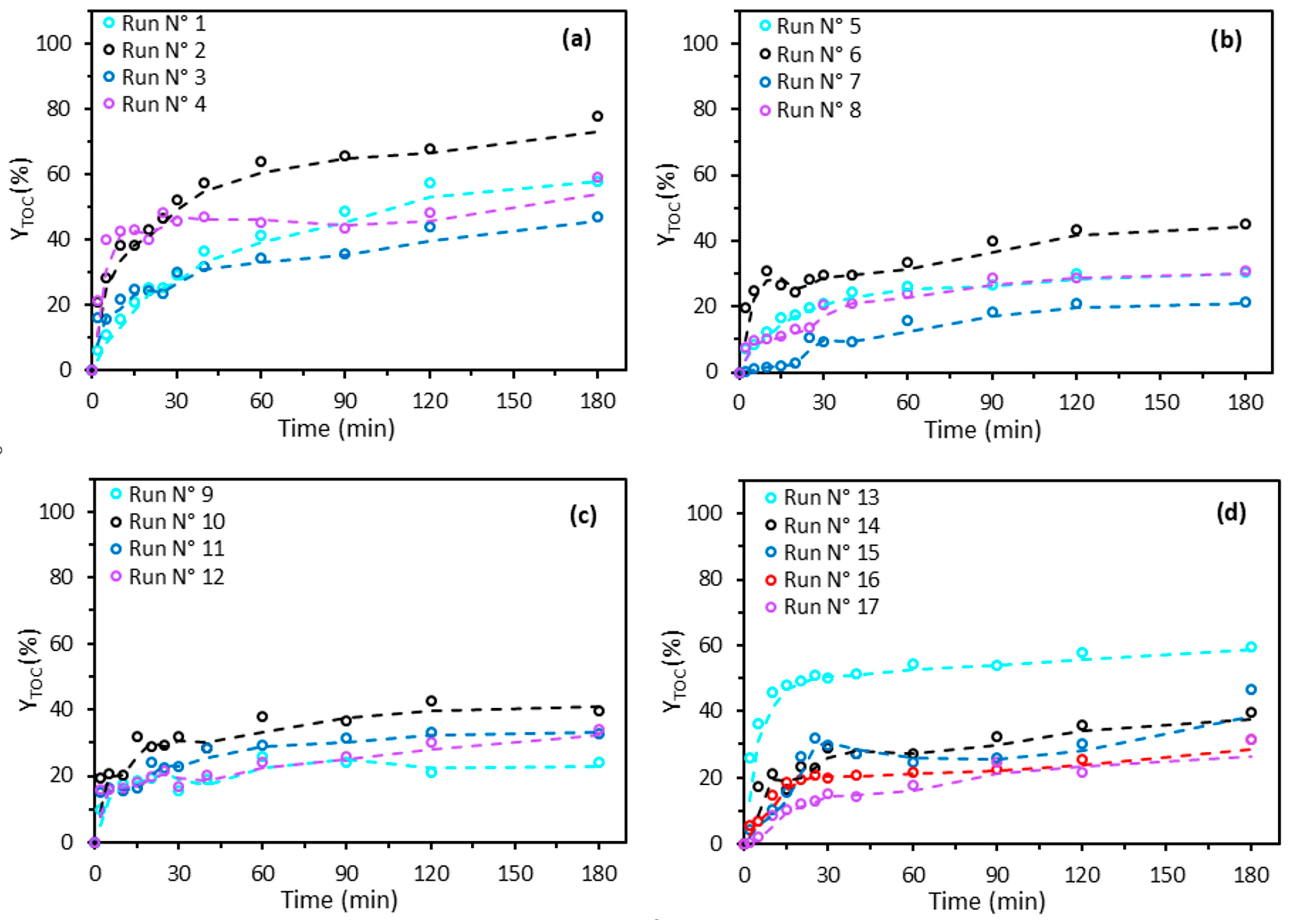
Figure 2 shows the evolution of the mineralization efficiency of 2,4-D (YTOC) over time for the 17 experiments. Overall, a two-phase kinetic behavior can be observed. The first phase corresponds to a relatively rapid increase in mineralization during the first 30 min, suggesting a fast initial reaction in which the pollutant is easily degradable. The second phase reveals a more gradual rise in the mineralization rate, with a near plateau from 120 to 180 min. This indicates slower degradation of the pollutant, potentially explained by the formation of 2,4-D residues or degradation by-products that are more recalcitrant and harder to break down. Similar findings have been reported in the literature for 2,4-D oxidation [16,26]. Furthermore, the presence of this near plateau suggests that beyond 180 min, any additional improvement in mineralization capacity is strongly limited.
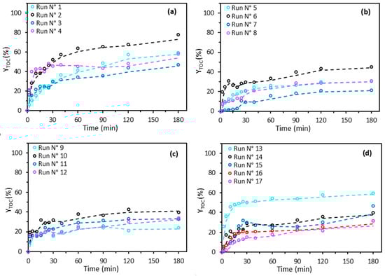
Figure 2.
TOC removal efficiency by the Fenton process. Experimental data shown in circles (○), and trend line shown in a dotted line (- -). (a) runs 1–4; (b) runs 5–8; (c) runs 9–12; (d) runs 13–17. According to the experimental design detailed in Table 3.
Run 2 (Figure 2a) exhibits the best performance after 180 min, with a final mineralization rate of 78%, followed by runs 1, 4 (Figure 2a), and 13 (Figure 2)), which reach 59% mineralization after 180 min. In contrast, runs 7 (Figure 2b) and 9 (Figure 2c) show much lower efficiency (21% and 24%, respectively). This difference in performance among the tests is mainly explained by the operating conditions, namely the L27-Fe dose, pH, and H2O2 dose (Table 2).
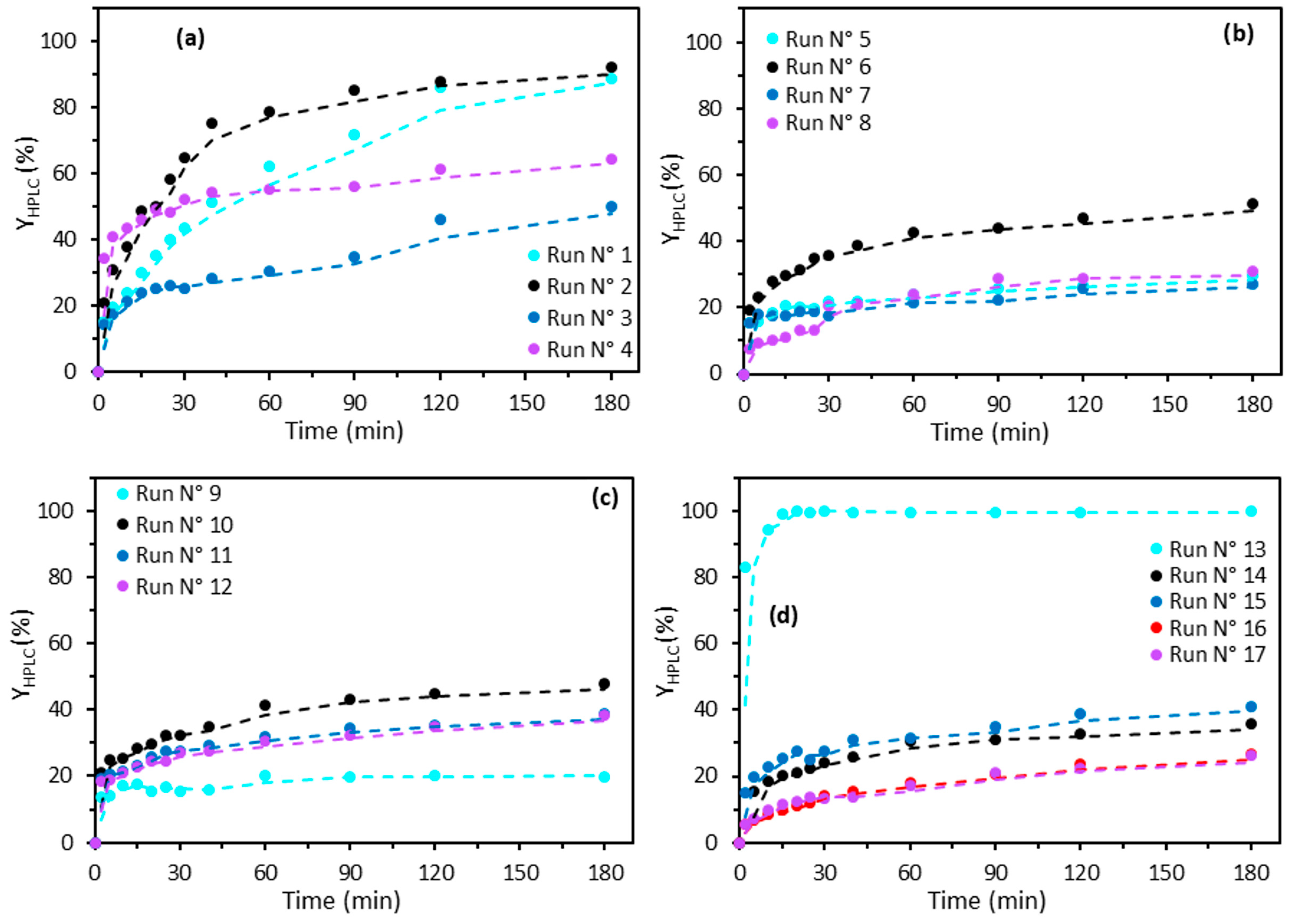
The degradation kinetics of 2,4-D by the Fenton process, monitored by HPLC (Figure 3), reveal higher degradation rates than those indicated by TOC analyses. This confirms the presence of degradation by-products not detected by HPLC but still measurable by the TOC meter. The works of Mohamed Ali [16] and Samba [26] have confirmed this trend.
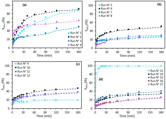
Figure 3.
HPLC removal efficiency by the Fenton process. Experimental data shown in circles (○), and trend line shown in a dotted line (- -). (a) runs 1–4; (b) runs 5–8; (c) runs 9–12; (d) runs 13–17. According to the experimental design detailed in Table 3.
3.1.1. Initial State of ANOVA Analysis
In order to evaluate the statistical significance of the main and interaction factors over the considered responses, an ANOVA analysis was carried out (Table 4 and Table A2). The independent variables were the dose of Fe-grafted AC (x1), dose of H2O2 (x2), and the solution pH (x3), whereas the process performance was evaluated based on the responses: 2,4-D removal efficiency (Y, %) after 10, 20, 30, 40, and 60 min of treatment.
Table 4.
ANOVA analysis for YTOC responses after different treatment durations.
Design Expert software (State-Ease Inc., Minneapolis, MN, USA, Version 7.1.5) was used to fit two second-order polynomial models to the spherical central composite design data.
In this phase of the initial ANOVA analysis, the unprocessed statistical models of YTOC had a freedom degree value of 9, whereas the freedom degree of residuals was 7, corresponding to a value for F tabulated/critic of 3.29. In order for the models to be statistically significant, the F-value should be higher than the F tabulated. Commonly, this condition is satisfied after removing the insignificant terms from the models. However, all five models meet the F-value > F tabulated condition. An interesting observation is that with the increase in treatment time, the F value increases significantly, strengthening the significance of the overall model describing the Fenton process. The same observation is also valid in the case of the p-value (low probabilities indicate high effects of the models; on the contrary, high probabilities that the null hypothesis is true, i.e., no factor effects, imply no significant effect). Based on the models of removal efficiencies at 10, 20, 30, and 60 min, the p-value decreases when treatment time increases in the order 0.0106 > 0.0103 > 0.0081 > 0.0031. However, the lowest p-value is reached after 40 min of treatment, 0.0008. While the first two models, at 10 and 20 min, are significant for a confidence interval of 95%, the subsequent three models have a more accurate confidence interval of 99%.
As already stated, the main goal of the present study was to screen the performance of the Fenton process over a wide and unbalanced range of values for the three considered independent values: Fe-grafted AC dose, H2O2 dose, and solution pH. However, it was quite difficult to ascertain why the H2O2 dose parameter has a relatively low effect on the overall performance of the Fenton process, especially in its early phase. Therefore, closer attention has been paid to the influence of this main parameter and its evolution during the Fenton treatment in terms of TOC.
First, it can be noted that all three main factors increase in statistical significance up to 60 min of treatment duration. The catalyst dose term has a p-value lower than 0.05 in the first 40 min, and at 60 min, it decreases below 0.01, thus strengthening its confidence interval up to 99%. The solution pH term presents the highest confidence interval from the beginning of the Fenton process, and even then, the positive evolution is still valid, with a lower and lower p-value until reaching values lower than 0.0001. The issues in terms of statistical significance within the chosen experimental ranges were recorded in the case of the H2O2 dose. In the first 30 min of treatment, it seems this parameter has a low influence over the process performance; its term gets significant at 90% confidence interval after 40 min, and becomes stronger (relevant at 95% confidence interval) after 60 min.
Among the many aspects considered in choosing the experimental design, special attention was given to the ratio of Fe ions and H2O2 dose, with its optimality standing around 1:10 [30]. Nevertheless, in the present study, the amount of AC support is quite high with respect to the aforementioned ratio. Consequently, at the beginning of each experimental run, the concurrent adsorptions of 2,4-D and H2O2 are very strong, shadowing the influence of H2O2 dose on the overall treatment process.
Quasi-similar findings are also valid in the case of YHPLC responses, as shown in Table A2.
3.1.2. ANOVA Analysis of Significant Terms
Table 5 shows the ANOVA analysis for YTOC responses at different treatment durations, after removing the insignificant terms. Each model quality of fitness was improved by removing the terms with high p-values (>0.1).
Table 5.
ANOVA analysis for YTOC responses after different treatment durations, after removing insignificant terms.
Keeping only the statistically significant terms that affect the responses, the following models (in coded terms) were determined:
Table 6 summarizes the main model indicators.
Table 6.
Statistics of the five obtained models.
Based on ANOVA analysis, it was found that all five suggested models can be validated by Fischer tests (model F-value higher than F-tabulated). Also, in terms of F-values, the lack of fit is statistically insignificant (LOF F-value lower than F-tabulated).
With the increase of treatment duration, the models describing removal efficiency in terms of TOC are more and more accurate. This is supported by the increase in the values corresponding to the determination coefficient and the adjusted and predicted determination coefficients. Also, the adequate precision indicator is several times higher than the value of four, and increases with treatment duration.
Except for the responses at 20 and 30 min of treatment, the three main factors are important in relation to Fenton process performance. As concerns the interaction factors, only that between the H2O2 dose and solution pH is statistically significant after 10 min of treatment. Independent from the treatment duration, the squared term of solution pH has an important effect on the removal efficiency, and only at the end of the Fenton process, after 60 min, the squared term of Fe-AC dose becomes significant.
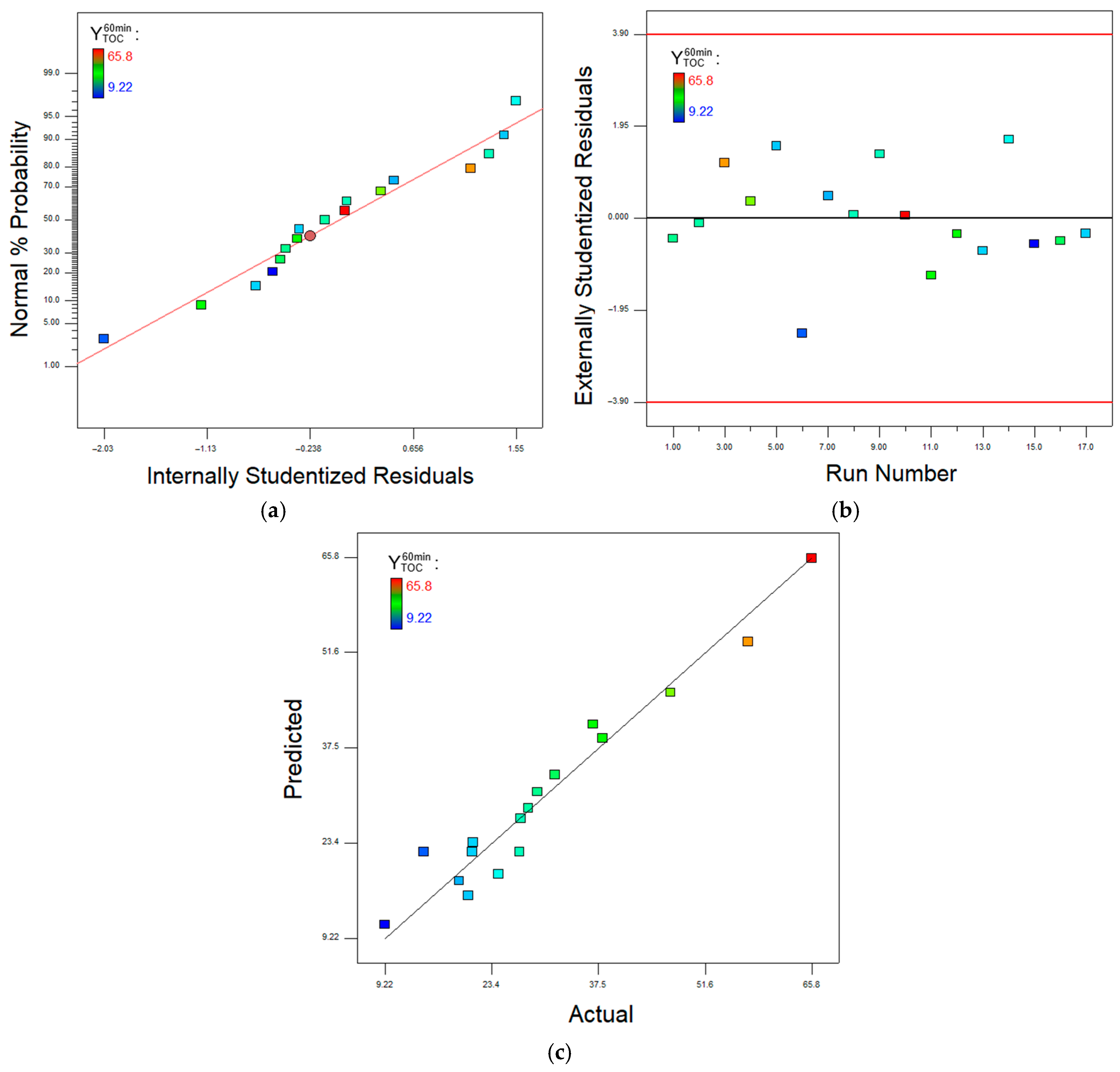
Figure 4 shows normal probability and residual plots as well as the agreement between predicted and experimental values of the responses after 60 min of Fenton process.
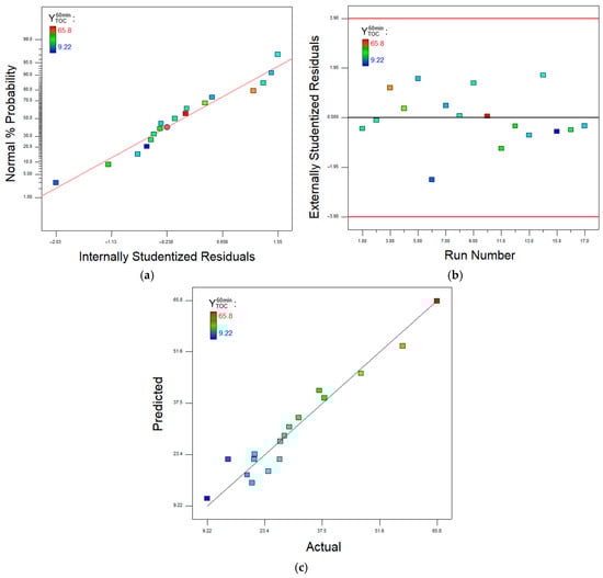
Figure 4.
Normal probability plot (a), residual plot (b), and predicted vs. experimental plot (c) for the removal efficiency in terms of TOC data, after 60 min of treatment.
Diagnostic plots show that the studentized residuals align on a straight line in the normal plot and present no trends and a random distribution in the residuals versus run number plot. The goodness of fit can be visualized in the data correlation of predicted versus actual plot.
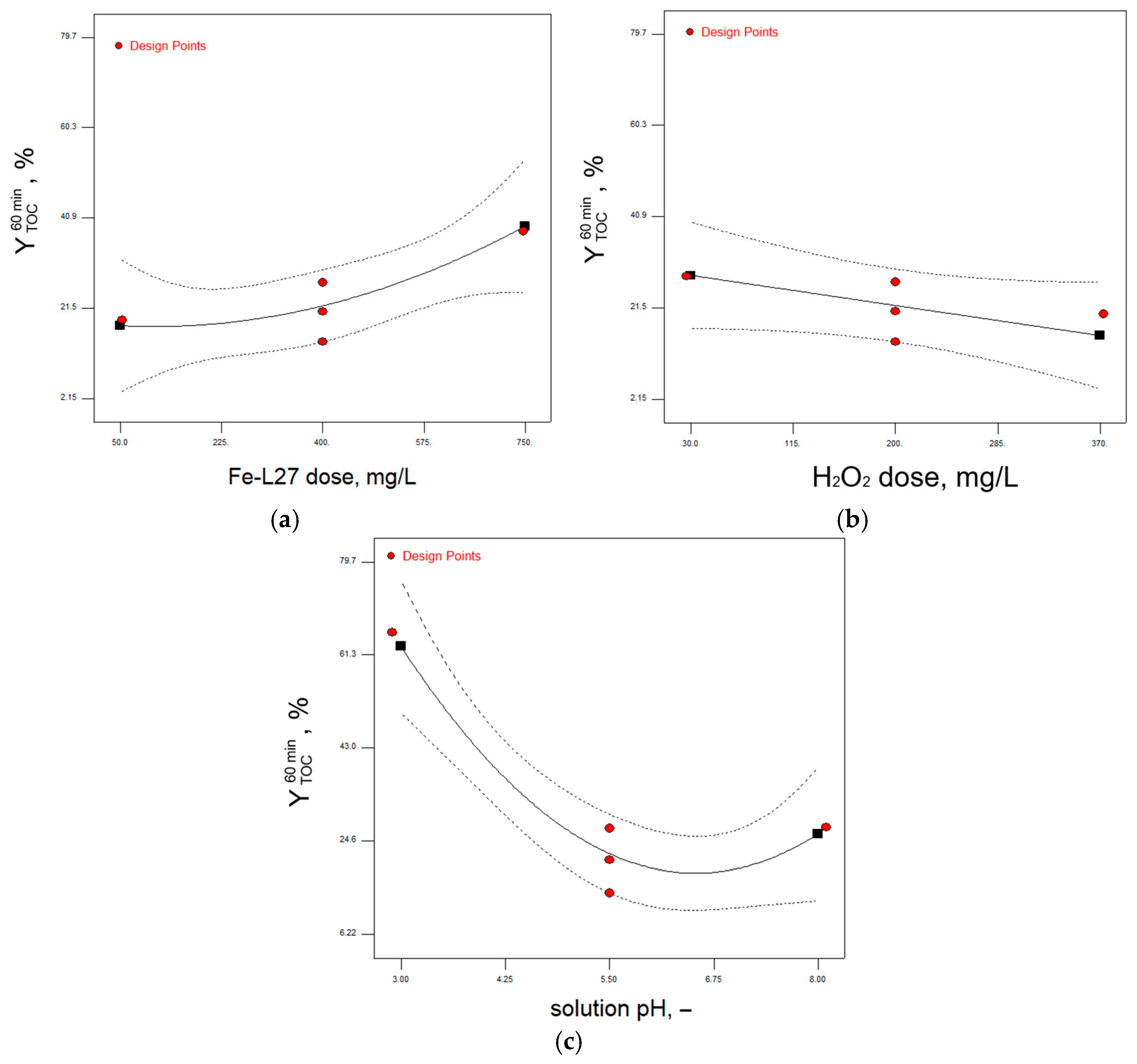
Figure 5 presents the effects of significant factors on the removal efficiency.
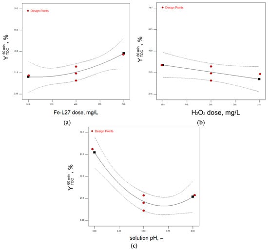
Figure 5.
Plots of marginal means of removal efficiency in relation to TOC after 60 min of treatment as influenced by (a) L27-Fe dose, (b) H2O2 dose, and (c) solution pH; solid line—suggested model; dashed line—confidence interval; ◼—predicted responses for each factor level.
The increase in the L27-Fe dose factor is reflected in a strong increase in the performance of the treatment process, the steeper slope stressing a stronger influence on the removal efficiency response. The H2O2 dose factor in the considered experimental range shows that the optimal ratio in relation to iron grafted on L27 AC has been reached towards the inferior value of 100 mg L−1 and below. As expected, the strongest influence in the degradation process of 2,4-D molecule is given by the solution pH factor. Thus, a decrease of solution pH below the value of 5 results in a steep increase in removal efficiency, with a local maximum a pH value of 2.9 (run 13, ).
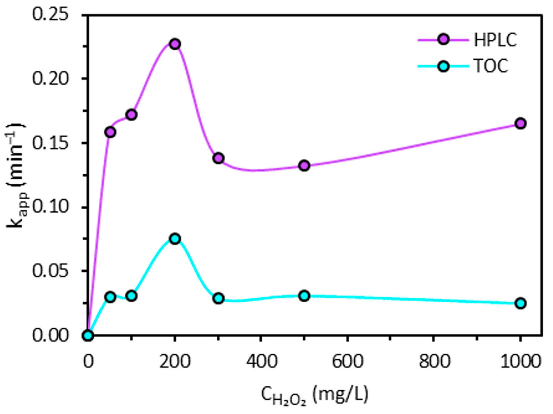
Figure 6 shows the influence of H2O2 dose on the apparent constant rate determined based on the first 10 min of the Fenton process. Seemingly, at the beginning of the Fenton process, H2O2 dose has an optimal value where the degradation of 2,4-D molecule reaches a maximum value for the apparent constant rate in close dependence to the concentration of iron grafted onto the L27 AC.
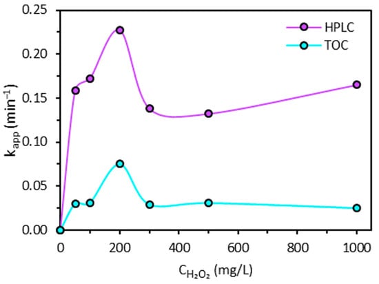
Figure 6.
Dependence of apparent constant rate of the Fenton process on the H2O2 dose according to HPLC and TOC analyses.
Design Expert software was also employed to determine the local optimum values for the removal efficiency in relation to TOC, after 60 min of treatment. The optimization method used by the software is described in reference [31]. Table 7 presents the optimization criteria for the considered response.
Table 7.
Summary of the main model indicators.
Among the three different cases considered in the optimization study, case#1 maximized the objective function for the entire experimental range. The removal efficiency in relation to TOC achieves a value of 78.5% with a maximal desirability corresponding to a L27-Fe dose of 730 mg L−1, a H2O2 concentration of 224 mg L−1, and at the known optimal solution pH of 2.98 [30]. The other two cases show optimal values of removal efficiency at a pH of 5.5 (45.4%) and at a pH value of 8.1 (49.3%).
3.2. Fenton-Peroxone Process
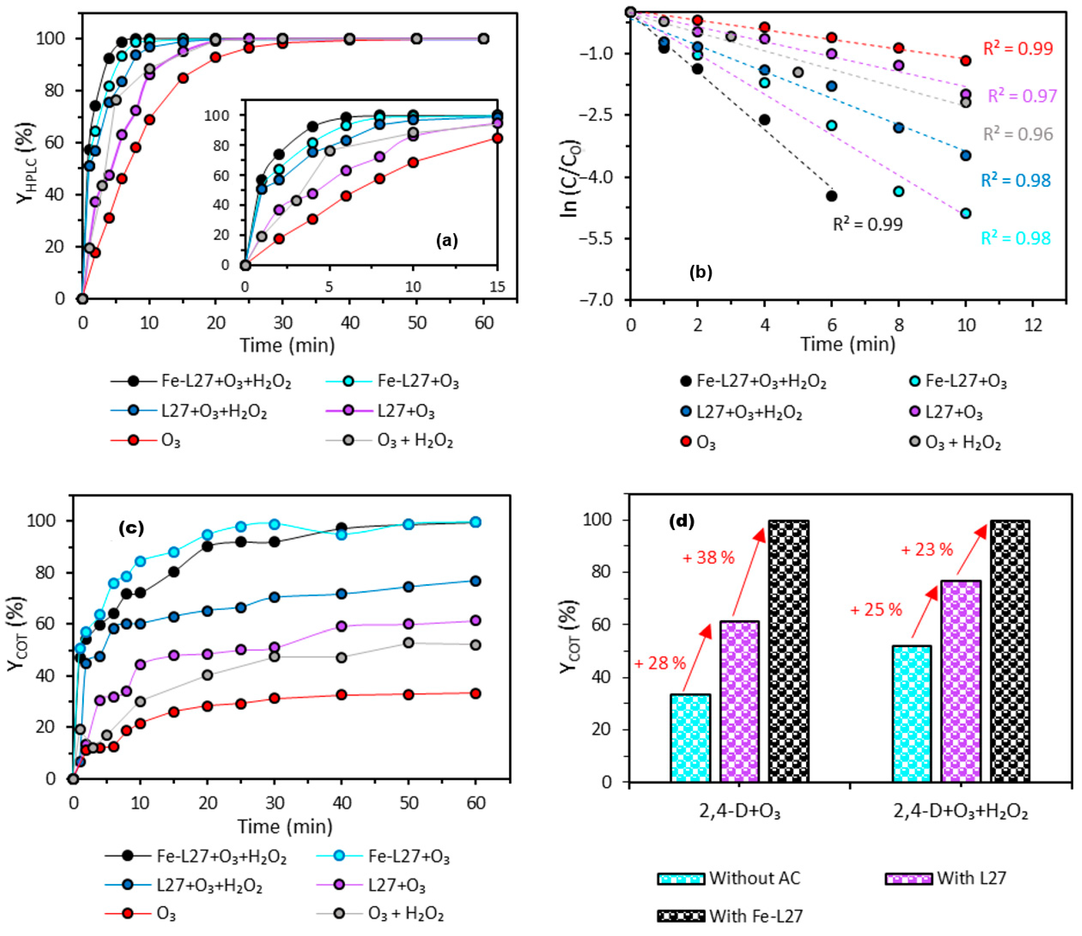
In order to achieve complete mineralization of 2,4-D, the Fenton process is coupled with ozonation. For this purpose, the experimental setup shown in Figure 1 was used. Briefly, the ozone concentration was fixed at 25 g·Nm−3 [26]. The treated solution had a volume of 500 mL, with an L27-Fe dose of 730 mg·L−1 and hydrogen peroxide (H2O2) at 224 mg·L−1, corresponding to the operating conditions of run 13 (Table 2). This experiment was the only one to achieve complete degradation of 2,4-D ( = 100%), although the mineralization remained limited to 59%. The degradation of 2,4-D by the Fenton–peroxone coupling was monitored over time by HPLC (Figure 7a), while mineralization was assessed by TOC analysis (Figure 7c). Lastly, the apparent degradation kinetics were modeled using a pseudo-first-order kinetic model (Figure 7b). To assess the impact of this coupling (O3 + H2O2) as well as the presence of iron on the carbon surface, the degradation of 2,4-D was systematically compared to that obtained by ozonation alone (O3), peroxonation (O3 + H2O2), and their combinations with either L27 or L27-Fe.
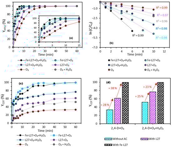
Figure 7.
(a) Degradation rate kinetics of 2,4-D monitored by HPLC. (b) Kinetic modeling of 2,4-D degradation according to the pseudo-first-order model. (c) Mineralization rate kinetics of 2,4-D. (d) Mineralization rate of 2,4-D as a function of the applied processes.
Figure 7a shows that, for all tested processes, 2,4-D degradation occurs relatively quickly, with degradation rates ranging from 69% to 100% within the first 10 min of treatment. The system combining Fe-L27, O3, and H2O2 demonstrates the highest efficiency, achieving complete degradation within 10 min (Table 8). In contrast, ozonation alone (O3) is the least effective because it relies on the direct action of ozone, with less generation of hydroxyl radicals or catalytic activation. In contrast, the combined processes enhance oxidation through multiple pathways, making them much more efficient. Several studies have reported similar findings when comparing the degradation of 2,4-D by ozonation and by other ozone-based combined processes. (O3/plasma, O3/Fe2+, O3/H2O2) [32,33,34,35].
Table 8.
Degradation and mineralization rate of 2,4-D at 10 min and 60 min according to different AOPs.
The addition of hydrogen peroxide and activated carbon significantly enhances 2,4-D degradation, suggesting a synergistic effect leading to a greater production of free radicals that drive the degradation of the molecule. The kinetic modeling curves (Figure 7b) fit the experimental data well (R2 values ranging from 0.96 to 0.99), confirming that the degradation follows a pseudo-first-order kinetic model as shown by various authors who have worked on pollutant degradation using advanced oxidation processes (AOPs) [32,36,37,38]. The evolution of the apparent rate constant (kapp) is consistent with the observed order of process efficiency: Fe-L27 + O3 + H2O2 > Fe-L27 + O3 > L27 + O3 + H2O2 > O3 + H2O2 > L27 + O3 > O3 alone.
Mineralization results (Figure 7c,d) reveal substantial differences among the tested processes. Complete mineralization (100%) is achieved after 60 min with the Fe-L27 + O3 + H2O2 and Fe-L27 + O3 systems, whereas the other processes exhibit significantly lower efficiencies (Figure 7d). These findings highlight the key catalytic role of iron, especially in its Fe2+ oxidation state, in promoting the generation of hydroxyl radicals. A non-exhaustive set of reactions contributing to OH° production is presented below [28,39,40,41]:
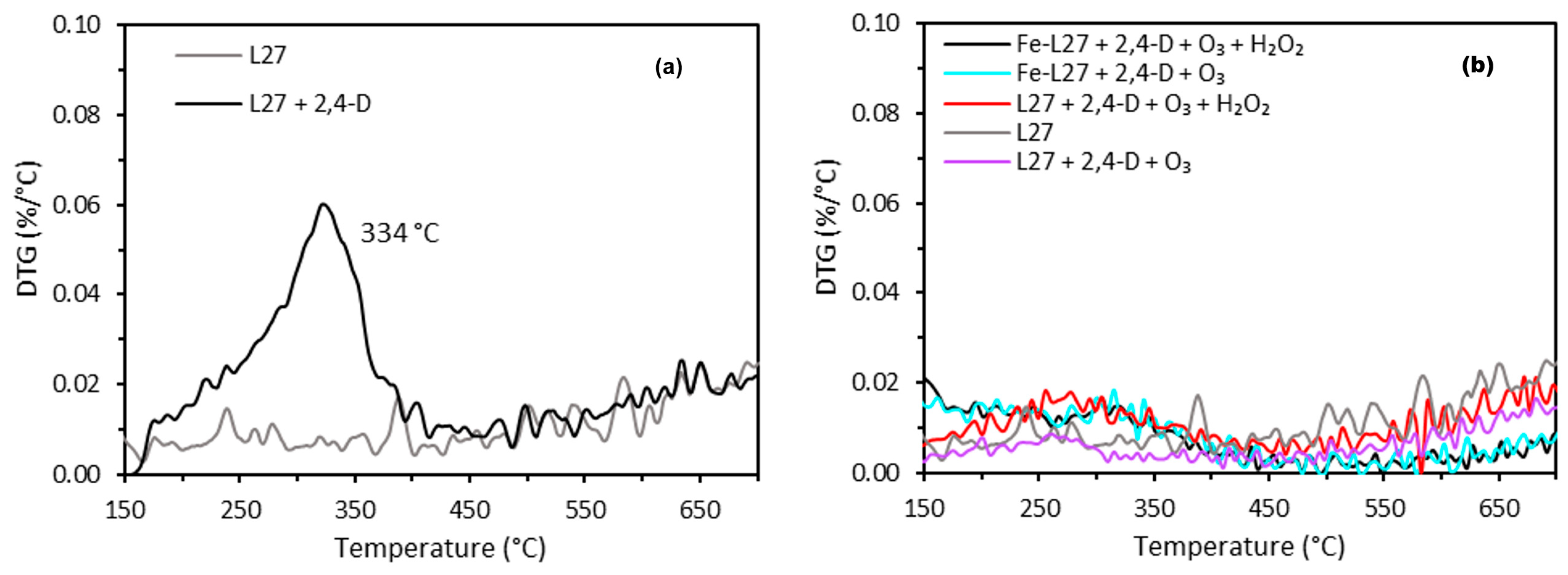
The results shown in Figure 8 highlight the beneficial impact of incorporating iron-enriched carbon-based catalytic materials (L27-Fe) into advanced oxidation processes (AOPs), particularly in enhancing the degradation and mineralization efficiencies of 2,4-D.

Figure 8.
Thermogravimetric analysis. (a) Activated carbon before and after 2,4-D adsorption and (b) activated carbon after 2,4-D treatment by advanced oxidation processes (AOPs).
This improvement is not merely the additive effect of ozone, hydrogen peroxide, and activated carbon used separately, but rather the result of a synergistic interaction between these three components. This synergy promotes a greater generation of hydroxyl radicals, enabling more extensive oxidation of the 2,4-D molecule. Furthermore, thermogravimetric analyses of the activated carbons after 60 min of 2,4-D treatment via the different AOPs (Figure 8) provide evidence of slight residual adsorption. Following a simple adsorption process on L27, for example, a distinct thermal desorption peak of 2,4-D is observed at 334 °C (Figure 8a), indicating substantial molecular adsorption onto the carbon material. In contrast, this desorption peak is nearly absent for samples treated with AOPs, suggesting that 2,4-D was largely degraded rather than merely adsorbed. A small residual desorption signal remains visible, particularly on L27 treated with O3 + H2O2 (red curve in Figure 8b), which may indicate partial adsorption or incomplete degradation under certain conditions. These findings support the conclusion that under AOP conditions, L27 and Fe-L27 function primarily as catalytic supports for oxidant activation rather than as passive adsorbents.
4. Conclusions
The degradation and mineralization of 2,4-D by the Fenton processes were studied at laboratory scale, and ozonation and coupling advanced oxidation processes were investigated at pilot scale. The catalyst used is developed from a commercial AC (L27) that has been enriched with iron. In order to determine the quantities of H2O2 and L27-Fe favorable for efficient mineralization, an experimental plant and a statistical study were carried out. These show an ideal dose of Fe-L27 of 730 mg·L−1 and an H2O2 dose of 224 mg·L−1. The application of ozonation processes alone has been shown to be effective for the complete degradation of 2,4-D, but is limited in terms of mineralization. The addition of H2O2 then allowed for the increase of the generation of hydroxyl radicals, resulting in a significant improvement of mineralization. The introduction of an activated carbon (L27) enhanced this performance in terms of mineralization, reflecting a favorable interaction between the surface of the AC and oxidizing species. The incorporation of iron as a catalyst (Fe-L27) led to the best performance, achieving complete mineralization after 60 min, accompanied by the highest kinetic constants. The catalytic support role of L27 in the system (Fe-L27) is evidenced by the absence of a desorption peak of 2,4-D on the TGA thermogram.
These results confirm the potential of the catalytic system Fe-L27 coupled to ozonation in the presence and absence of H2O2 as an effective solution for the treatment of organic pollutants in water. Future investigations will allow us to evaluate its stability in treatment cycles, its efficiency in complex matrices, and to study other processes of elaboration of Fe-AC systems like the ionothermal carbonization (ITC).
Author Contributions
P.F.S.: methodology, formal analysis, investigation, and writing—original draft preparation; M.S.S.: conceptualization, methodology, formal analysis, data curation, validation, writing—review and editing, and publication funding acquisition; S.S.: methodology, formal analysis, investigation, validation, and writing—review and editing; B.C.: conceptualization, methodology, validation, and writing—review and editing, resources, supervision. All authors have read and agreed to the published version of the manuscript.
Funding
This research was funded by Region Centre Val de Loire.
Data Availability Statement
The original contributions presented in this study are included in the article. Further inquiries can be directed to the corresponding authors.
Acknowledgments
The authors thank Jacobi Carbon for supplying the activated carbons and Jimmy Nicolle for the XPS analyses.
Conflicts of Interest
The authors declare no conflicts of interest.
Appendix A
Table A1.
Spherical (α = 1.73205)—CCD experimental design and the predicted and observed values of responses YHPLC 10–50 min.
Table A1.
Spherical (α = 1.73205)—CCD experimental design and the predicted and observed values of responses YHPLC 10–50 min.
| Run No. | Input Variables | Responses | |||||
|---|---|---|---|---|---|---|---|
| x1 | x2 | x3 | , % | , % | , % | , % | |
| 1 | −1 | −1 | −1 | 24 | 35 | 43 | 51 |
| 2 | 1 | −1 | −1 | 38 | 50 | 65 | 75 |
| 3 | −1 | 1 | −1 | 21 | 25 | 25 | 28 |
| 4 | 1 | 1 | −1 | 44 | 49 | 52 | 54 |
| 5 | −1 | −1 | 1 | 19 | 20 | 22 | 22 |
| 6 | 1 | −1 | 1 | 28 | 31 | 36 | 39 |
| 7 | −1 | 1 | 1 | 18 | 19 | 18 | 21 |
| 8 | 1 | 1 | 1 | 22 | 24 | 29 | 32 |
| 9 | −1.732 | 0 | 0 | 17 | 16 | 16 | 16 |
| 10 | 1.732 | 0 | 0 | 26 | 30 | 35 | 41 |
| 11 | 0 | −1.732 | 0 | 21 | 26 | 28 | 29 |
| 12 | 0 | 1.732 | 0 | 21 | 25 | 27 | 27 |
| 13 | 0 | 0 | −1.732 | 90 | 99 | 100 | 99 |
| 14 | 0 | 0 | 1.732 | 18 | 21 | 24 | 26 |
| 15 | 0 | 0 | 0 | 23 | 28 | 28 | 31 |
| 16 | 0 | 0 | 0 | 9 | 11 | 14 | 15 |
| 17 | 0 | 0 | 0 | 10 | 12 | 13 | 14 |
Table A2.
ANOVA analysis for YHPLC responses after different treatment durations.
Table A2.
ANOVA analysis for YHPLC responses after different treatment durations.
| Source | Sum of Square; Degrees of Freedom; F-Value; p-Value × 102 | ||||
|---|---|---|---|---|---|
| , % | , % | , % | , % | ||
| Model | 4350; 9; 2.97; 8.24 *** | 6150; 9; 5.60; 1.67 ** | 7070; 9; 8.42; 0.52 * | 7980; 9; 13; 0.14 * | 10,500; 9; 9.44; 0.37 * |
| x1 | 297; 1; 0.22; 22.8 | 455; 1; 3.73; 9.46 *** | 826; 1; 8.85; 2.06 ** | 1060; 1; 15.5; 0.57 * | 1160; 1; 9.43; 1.8 ** |
| x2 | 1.54; 1; 0.93; 92.5 | 33.5; 1; 0.28; 61.6 | 126; 1; 1.35; 28.4 | 212; 1; 3.11; 12.1 | 394; 1; 3.2; 11.7 |
| x3 | 1940; 1; 12; 1.05 ** | 2890; 1; 23.7; 0.18 * | 3240; 1; 34.8; 0.06 * | 3550; 1; 51.9; 0.02 * | 3810; 1; 31; 0.08 * |
| x1x2 | 1.71; 1; 0.01; 92.1 | 1.03; 1; 0.008; 92.9 | 1.14; 1; 0.01; 91.5 | 1.77; 1; 0.03; 87.7 | 27; 1; 0.22; 65.4 |
| x1x3 | 63.8; 1; 0.39; 55.1 | 63.8; 1; 0.52; 49.3 | 65; 1; 0.70; 43.2 | 58.6; 1; 0.86; 38.6 | 232; 1; 1.89; 21.2 |
| x2x3 | 12.6; 1; 0.08; 78.9 | 0.46; 1; 0.004; 95.3 | 50.7; 1; 0.54; 48.5 | 171; 1; 2.49; 15.8 | 441; 1; 3.58; 10 |
| x12 | 25.9; 1; 0.16; 70.2 | 55.4; 1; 0.45; 52.2 | 81; 1; 0.87; 38.3 | 200; 1; 2.92; 13.1 | 680; 1; 5.52; 5.11 *** |
| x22 | 23.2; 1; 0.14; 71.7 | 109; 1; 0.89; 37.6 | 133; 1; 1.43; 27.1 | 192; 1; 2.8; 13.8 | 1100; 1; 8.93; 2.03 ** |
| x32 | 1883; 1; 11.5; 1.15 ** | 2600; 1; 21.3; 0.24 * | 2670; 1; 28.6; 0.11 * | 2900; 1; 42.5; 0.03 * | 4210; 1; 34.2; 0.06 * |
| Residual | 1140; 7 | 853; 7 | 653; 7 | 479; 7 | 861; 7 |
| Lack of Fit | 1010; 5; 3.2; 25.5 | 828; 5; 12.8; 7.4 | 612; 5; 5.91; 15.1 | 447; 5; 5.54; 16 | 787; 5; 4.22; 20.3 |
| Pure Error | 126; 2 | 25.9; 2 | 41.4; 2 | 32; 2 | 74.6; 2 |
* significant for a confidence level of 99%; ** significant for a confidence level of 95%; *** significant for a confidence level of 90%.
References
- Ullah, S.; Shah, S.S.A.; Altaf, M.; Hossain, I.; El Sayed, M.E.; Kallel, M.; El-Bahy, Z.M.; Rehman, A.U.; Najam, T.; Nazir, M.A. Activated Carbon Derived from Biomass for Wastewater Treatment: Synthesis, Application and Future Challenges. J. Anal. Appl. Pyrolysis 2024, 179, 106480. [Google Scholar] [CrossRef]
- Gomis-Berenguer, A.; Sidoli, P.; Cagnon, B. Adsorption of Metolachlor and Its Transformation Products, ESA and OXA, on Activated Carbons. Appl. Sci. 2021, 11, 7342. [Google Scholar] [CrossRef]
- Yang, G.; Chen, H.; Qin, H.; Feng, Y. Amination of Activated Carbon for Enhancing Phenol Adsorption: Effect of Nitrogen-Containing Functional Groups. Appl. Surf. Sci. 2014, 293, 299–305. [Google Scholar] [CrossRef]
- Liu, W.; Zhang, Y.; Wang, S.; Bai, L.; Deng, Y.; Tao, J. Effect of Pore Size Distribution and Amination on Adsorption Capacities of Polymeric Adsorbents. Molecules 2021, 26, 5267. [Google Scholar] [CrossRef] [PubMed]
- Samba, P.; Schaefer, S.; Cagnon, B. Impregnation by Hydrothermal Carbonization in the Presence of Phosphoric Acid in the Activated Carbon Production Process from Hemp Residues: Impact on Porous Properties and Ibuprofen Adsorption. J. Ind. Eng. Chem. 2025, in press. [Google Scholar] [CrossRef]
- Li, P.; Yin, Z.; Chi, C.; Wang, Y.; Wang, Y.; Liu, H.; Lv, Y.; Jiang, N.; Wu, S. Treatment of Membrane-Concentrated Landfill Leachate by Heterogeneous Chemical and Electrical Fenton Processes with Iron-Loaded Granular Activated Carbon Catalysts. J. Environ. Chem. Eng. 2024, 12, 112337. [Google Scholar] [CrossRef]
- López-Francés, A.; Cabrero-Antonino, M.; Bernat-Quesada, F.; Ferrer, B.; Blanes, M.; García, R.; Almenar, P.; Álvaro, M.; Dhakshinamoorthy, A.; Baldoví, H.G.; et al. Valorization of Field-Spent Granular Activated Carbon as Heterogeneous Ozonation Catalyst for Water Treatment. ChemSusChem 2024, 17, e202400062. [Google Scholar] [CrossRef]
- Zhang, X.; Xue, X.; Hu, J. Combined Ozonation-Biological Activated Carbon Process for Antibiotic Resistance Control in Treated Effluent from Wastewater Treatment Plant. Water Res. 2025, 268, 122610. [Google Scholar] [CrossRef]
- Gholizadeh, A.M.; Zarei, M.; Ebratkhahan, M.; Hasanzadeh, A. Phenazopyridine Degradation by Electro-Fenton Process with Magnetite Nanoparticles-Activated Carbon Cathode, Artificial Neural Networks Modeling. J. Environ. Chem. Eng. 2021, 9, 104999. [Google Scholar] [CrossRef]
- Ren, S.; Zhang, Y.; Wang, A.; Song, Y.; Zhang, N.; Wen, Z.; Liu, Y.; Fan, R.; Zhang, Z. Efficient Mineralization of Sulfamethoxazole by a Tandem Dual-System Electro-Fenton Process Using a Gas Diffusion Electrode for H2O2 Generation and an Activated Carbon Fiber Cathode for Fe2+ Regeneration. Sep. Purif. Technol. 2025, 354, 129108. [Google Scholar] [CrossRef]
- Zhang, M.; Dong, H.; Zhao, L.; Wang, D.; Meng, D. A Review on Fenton Process for Organic Wastewater Treatment Based on Optimization Perspective. Sci. Total Environ. 2019, 670, 110–121. [Google Scholar] [CrossRef] [PubMed]
- Nguyen, M.L.; Ngo, H.L.; Hoang, T.T.N.; Le, D.T.; Nguyen, D.D.; Huynh, Q.S.; Nguyen, T.T.T.; Nguyen, T.T.; Juang, R.-S. Effective Degradation of Tetracycline in Aqueous Solution by an Electro-Fenton Process Using Chemically Modified Carbon/α-FeOOH as Catalyst. J. Environ. Health Sci. Eng. 2024, 22, 313–327. [Google Scholar] [CrossRef] [PubMed]
- Kamenická, B.; Weidlich, T. A Comparison of Different Reagents Applicable for Destroying Halogenated Anionic Textile Dye Mordant Blue 9 in Polluted Aqueous Streams. Catalysts 2023, 13, 460. [Google Scholar] [CrossRef]
- Gurav, R.; Mandal, S.; Smith, L.M.; Shi, S.Q.; Hwang, S. The Potential of Self-Activated Carbon for Adsorptive Removal of Toxic Phenoxyacetic Acid Herbicide from Water. Chemosphere 2023, 339, 139715. [Google Scholar] [CrossRef]
- Ma, W.; Fan, J.; Cui, X.; Wang, Y.; Yan, Y.; Meng, Z.; Gao, H.; Lu, R.; Zhou, W. Pyrolyse Du Marc de Café Usagé En Biochar Traité Avec H3PO4 Pour l’élimination Efficace de l’herbicide Acide 2,4-Dichlorophénoxyacétique: Comportements et Mécanisme d’adsorption. J. Environ. Chem. Eng. 2023, 11, 109165. [Google Scholar] [CrossRef]
- Ali, A.M. Etude d’un Procédé d’oxydation Avancée Couplé Plasma Non Thermique/Carbone Activé Fonctionnalisé Pour Le Traitement d’herbicides Dans l’eau. Ph.D. Thesis, Université d’Orléans, Orléans, France, 2024. [Google Scholar]
- Gupta, T.; Rawat, A.; Das, J.; Sahoo, P.K.; Mohanty, P. Efficient Removal of Herbicide 2,4-Dichlorophenoxyacetic Acid from Aqueous Solution Investigated by Batch, Column, and Membrane Separation Methods. Sep. Purif. Technol. 2025, 360, 130868. [Google Scholar] [CrossRef]
- Ebrahimi, R.; Maleki, A.; Rezaee, R.; Daraei, H.; Safari, M.; McKay, G.; Lee, S.-M.; Jafari, A. Synthesis and Application of Fe-Doped TiO2 Nanoparticles for Photodegradation of 2,4-D from Aqueous Solution. Arab. J. Sci. Eng. 2021, 46, 6409–6422. [Google Scholar] [CrossRef]
- Loomis, D.; Guyton, K.; Grosse, Y.; Ghissasi, F.E.; Bouvard, V.; Benbrahim-Tallaa, L.; Guha, N.; Mattock, H.; Straif, K. Carcinogenicity of Lindane, DDT, and 2,4-Dichlorophenoxyacetic Acid. Lancet Oncol. 2015, 16, 891–892. [Google Scholar] [CrossRef]
- Boumaraf, R.; Khettaf, S.; Benmahdi, F.; Masmoudi, R.; Ferhati, A. Removal of 2,4-Dichlorophenoxyacetic Acid from Aqueous Solutions by Nanofiltration and Activated Carbon. Biomass Convers. Biorefinery 2024, 14, 15689–15704. [Google Scholar] [CrossRef]
- Muhammad, J.B.; Shehu, D.; Usman, S.; Dankaka, S.M.; Gimba, M.Y.; Jagaba, A.H. Potentiel de Biodégradation de l’acide 2,4 Dichlorophénoxyacétique Par Cupriavidus Campinensis Isolé Du Sol Cultivé Dans Une Rizière. Case Stud. Chem. Environ. Eng. 2023, 8, 100434. [Google Scholar] [CrossRef]
- Zhu, K.; Sun, C.; Chen, H.; Baig, S.A.; Sheng, T.; Xu, X. Enhanced Catalytic Hydrodechlorination of 2,4-Dichlorophenoxyacetic Acid by Nanoscale Zero Valent Iron with Electrochemical Technique Using a Palladium/Nickel Foam Electrode. Chem. Eng. J. 2013, 223, 192–199. [Google Scholar] [CrossRef]
- Secula, M.S.; Vajda, A.; Cagnon, B.; Warmont, F.; Mamaliga, I. Photo-Fenton-Peroxide Process Using FE (II)-Embedded Composites Based on Activated Carbon: Characterization of Catalytic Tests. Can. J. Chem. Eng. 2020, 98, 650–658. [Google Scholar] [CrossRef]
- Jagiello, J.; Olivier, J.P. Carbon Slit Pore Model Incorporating Surface Energetical Heterogeneity and Geometrical Corrugation. Adsorption 2013, 19, 777–783. [Google Scholar] [CrossRef]
- de Oliveira, T.F.F. Etude d’un Procédé de Dépollution Basé Sur Le Couplage Ozone/Charbon Actif Pour l’élimination Des Phtalates En Phase Aqueuse. Ph.D. Thesis, Université d’Orléans, Orléans, France, 2011. [Google Scholar]
- Samba, P. Elaboration d’une nouvelle gamme de matériaux carbonés à partir de résidus lignocellulosiques par carbonisation solvo-thermale pour leur intégration dans des procédés d’oxydation avancée pour le traitement de l’eau. Ph.D. Thesis, Université d’Orléans, Orléans, France, 2024. [Google Scholar]
- Borman, P.; Elder, D. Q2(R1) Validation of Analytical Procedures: Text and Methodology. In ICH Quality Guidelines; Teasdale, A., Elder, D., Nims, R.W., Eds.; Wiley: Hoboken, NJ, USA, 2017; pp. 127–166. ISBN 978-1-118-97111-6. [Google Scholar]
- Staehelin, J.; Hoigne, J. Decomposition of Ozone in Water: Rate of Initiation by Hydroxide Ions and Hydrogen Peroxide. Environ. Sci. Technol. 1982, 16, 676–681. [Google Scholar] [CrossRef]
- von Gunten, U. Ozonation of Drinking Water: Part I. Oxidation Kinetics and Product Formation. Water Res. 2003, 37, 1443–1467. [Google Scholar] [CrossRef]
- Secula, M.S.; Suditu, G.D.; Poulios, I.; Cojocaru, C.; Cretescu, I. Response Surface Optimization of the Photocatalytic Decolorization of a Simulated Dyestuff Effluent. Chem. Eng. J. 2008, 141, 18–26. [Google Scholar] [CrossRef]
- Secula, M.S.; Stan, C.S.; Cojocaru, C.; Cagnon, B.; Cretescu, I. Multi-Objective Optimization of Indigo Carmine Removal by an Electrocoagulation/GAC Coupling Process in a Batch Reactor. Sep. Sci. Technol. 2014, 49, 924–938. [Google Scholar] [CrossRef]
- Bradu, C.; Magureanu, M.; Parvulescu, V.I. Degradation of the Chlorophenoxyacetic Herbicide 2,4-D by Plasma-Ozonation System. J. Hazard. Mater. 2017, 336, 52–56. [Google Scholar] [CrossRef]
- Yu, Y.; Ma, J.; Hou, Y. Degradation of 2,4-Dichlorophenoxyacetic Acid in Water by Ozone-Hydrogen Peroxide Process. J. Environ. Sci. 2006, 18, 1043–1049. [Google Scholar] [CrossRef]
- Aziz, K.H.H.; Miessner, H.; Mueller, S.; Mahyar, A.; Kalass, D.; Moeller, D.; Khorshid, I.; Rashid, M.A.M. Comparative Study on 2,4-Dichlorophenoxyacetic Acid and 2,4-Dichlorophenol Removal from Aqueous Solutions via Ozonation, Photocatalysis and Non-Thermal Plasma Using a Planar Falling Film Reactor. J. Hazard. Mater. 2018, 343, 107–115. [Google Scholar] [CrossRef]
- Brillas, E.; Calpe, J.C.; Cabot, P.-L. Degradation of the Herbicide 2,4-Dichlorophenoxyacetic Acid by Ozonation Catalyzed with Fe2+ and UVA Light. Appl. Catal. B Environ. 2003, 46, 381–391. [Google Scholar] [CrossRef]
- Chedeville, O.; Di Giusto, A.; Delpeux, S.; Cagnon, B. Oxidation of Pharmaceutical Compounds by Ozonation and Ozone/Activated Carbon Coupling: A Kinetic Approach. Desalination Water Treat. 2016, 57, 18956–18963. [Google Scholar] [CrossRef]
- Ivanets, A.; Prozorovich, V.; Roshchina, M.; Grigoraviciute-Puroniene, I.; Zarkov, A.; Kareiva, A.; Wang, Z.; Srivastava, V.; Sillanpää, M. Heterogeneous Fenton Oxidation Using Magnesium Ferrite Nanoparticles for Ibuprofen Removal from Wastewater: Optimization and Kinetics Studies. J. Nanomater. 2020, 2020, e8159628. [Google Scholar] [CrossRef]
- Brillas, E. A Critical Review on Ibuprofen Removal from Synthetic Waters, Natural Waters, and Real Wastewaters by Advanced Oxidation Processes. Chemosphere 2022, 286, 131849. [Google Scholar] [CrossRef]
- Hoigné, J.; Bader, H. The Role of Hydroxyl Radical Reactions in Ozonation Processes in Aqueous Solutions. Water Res. 1976, 10, 377–386. [Google Scholar] [CrossRef]
- Haber, F.; Weiss, J. The Catalytic Decomposition of Hydrogen Peroxide by Iron Salts. Proc. R. Soc. Lond. Ser. A—Math. Phys. Sci. 1934, 147, 332–351. [Google Scholar] [CrossRef]
- Loegager, T.; Holcman, J.; Sehested, K.; Pedersen, T. Oxidation of Ferrous Ions by Ozone in Acidic Solutions. Inorg. Chem. 1992, 31, 3523–3529. [Google Scholar] [CrossRef]
Disclaimer/Publisher’s Note: The statements, opinions and data contained in all publications are solely those of the individual author(s) and contributor(s) and not of MDPI and/or the editor(s). MDPI and/or the editor(s) disclaim responsibility for any injury to people or property resulting from any ideas, methods, instructions or products referred to in the content. |
© 2025 by the authors. Licensee MDPI, Basel, Switzerland. This article is an open access article distributed under the terms and conditions of the Creative Commons Attribution (CC BY) license (https://creativecommons.org/licenses/by/4.0/).