Tunnel Lining Recognition and Thickness Estimation via Optical Image to Radar Image Transfer Learning

Abstract

The secondary lining of a tunnel is a critical load-bearing component, whose stability and structural integrity are essential for ensuring the overall safety of the tunnel. However, identifying lining structures and estimating their thickness using ground-penetrating radar (GPR) remain challenging due to several inherent limitations. First, the limited electromagnetic contrast between the primary and secondary linings results in weak interface reflections in GPR imagery, thereby hindering accurate delineation. Second, construction errors such as over-excavation or under-excavation often lead to complex interface geometries, further complicating the interpretation of GPR signals. To address these challenges, we propose an enhanced YOLOv8-seg network capable of performing pixel-level segmentation on GPR images to accurately delineate secondary lining regions and estimate their thickness. The model integrates a convolutional block attention module (CBAM) to refine feature extraction by emphasizing critical characteristics of the two interface layers through channel-wise and spatial attention mechanisms. The model is first pretrained on the COCO dataset and subsequently fine-tuned via transfer learning using a hybrid GPR dataset comprising real-world measurements and numerically simulated data based on forward modeling. Finally, the model is validated on real-world GPR measurements acquired from the Longhai tunnel. Experimental results demonstrate that the proposed method reliably identifies secondary tunnel linings and accurately estimates their average thickness.

1. Introduction

In tunnel engineering, the lining plays a critical role in withstanding the surrounding rock pressure and its own weight to maintain tunnel stability [1]. A lining thickness thinner than the design specification may pose potential risks to the tunnel structure [2]. Compared to traditional methods such as sampling and impact testing, GPR technology has gained widespread application in tunnel lining inspection due to its advantages of being non-destructive and efficient [3]. However, since the acquired GPR data consists of reflected electromagnetic waves from the underground environment rather than direct imaging of the tunnel lining structure, extensive data processing is required to characterize the internal structure [4]. Therefore, there is a need for an automatic recognition algorithm to enhance the interpretability of GPR data.

With the advent of convolutional neural networks (CNNs), deep learning techniques have made significant advances in the detection of secondary tunnel lining thickness. CNNs possess the capability to learn high-level image features, enabling the automated interpretation of GPR images. Among these, the R-CNN and YOLO series are commonly employed for tunnel lining detection. In 2021, Qin et al. proposed a deep learning-based automatic recognition method that integrates Mask R-CNN with the finite-difference time-domain (FDTD) method and DCGAN-based data augmentation. The model was trained on 28,600 synthetic and 118 real GPR images, achieving the automated identification of tunnel lining elements. Due to the significant discrepancy between the reflection signals in GPR images and actual geometric features, the method did not explicitly delineate structural contours. Instead, bounding boxes were used to annotate the approximate positions and extents of the targets [5]. In the same year, Li et al. developed a deep learning-based non-destructive evaluation method that integrates GPR and electromagnetic induction (EMI) data. Using YOLOv3 and a 1D CNN, the method achieved the high-precision automated estimation of rebar diameters and protective layer thicknesses [6]. In 2022, Wang et al. proposed a method based on a Rotated Region Deformable Convolutional Neural Network (R2DCNN), trained on both synthetic and real GPR datasets to detect internal defects and rebars in arbitrary orientations within tunnel linings. However, the model has not yet been validated on large-scale and diverse real-world datasets, and the current results may not fully reflect its generalizability across various practical scenarios [7]. That same year, Rosso et al. introduced a deep learning framework combining CNN and Vision Transformer (ViT) architectures, trained on 27,890 GPR images, to achieve the automatic classification of highway tunnel defects. However, its high computational requirements limit its potential for real-time monitoring on low-power edge devices [8]. In 2023, Huang et al. proposed a deep learning framework based on SA-DenseCL that incorporates self-supervised learning to reduce dependence on annotated data. A limited set of labeled GPR images was used to fine-tune Mask R-CNN for estimating rebar distribution, void defect locations, and secondary lining thickness. However, its heavy computational burden during the pretraining phase restricts its deployment in resource-constrained environments [9]. That same year, Liu et al. introduced an integrated method based on M-YOLACT, which employed a multi-task deep neural network along with curve-fitting post-processing to simultaneously identify tunnel lining defects and estimate both defect depth and lining thickness from GPR images [10]. In 2024, Yue et al. developed a YOLOP-based algorithm and applied transfer learning using a dataset containing three types of underground targets: rebar in concrete, buried pipelines, and hidden defects behind shield tunnel linings. The model enabled the automatic detection of defects behind railway tunnel linings and estimation of their thickness [11]. Also in 2024, Zhao et al. proposed a deep learning-based dynamic wave detection framework for multi-defect recognition in tunnel lining GPR images. A multidimensional defect dataset was generated using the TLGAN image synthesis network, and a Wave-DetNets detection model—built upon wave function theory and YOLOv5—was developed to achieve efficient identification and localization of multiple defect types [12].

This study proposes an improved network model based on YOLOv8-seg, which leverages deep CNNs to extract features from GPR images. It integrates strong localization features from low-level feature maps with precise localization information from high-level feature maps, aggregates parameters across different backbone layers to enhance the representation of multi-scale features, and ultimately performs pixel-level segmentation to identify the secondary lining region in GPR images and estimate its thickness.

2. The Tunnel GPR Dataset and Transfer Learning Between Optical and Radar Images

The tunnel GPR dataset used in this study was collected from the Longhai tunnel of the Zhangjiuhe Water Diversion Project using a SIR-3000 ground-penetrating radar system with a central frequency of 900 MHz. During field testing, calibration experiments were conducted by laying GPR survey lines over tunnel lining sections with known thicknesses. The relative permittivity of the cast-in-place reinforced concrete used in the project was derived by measuring the electromagnetic wave travel time and correlating it with the actual lining thickness. The calibrated value was determined to be 6.3. Based on the reflection characteristics of electromagnetic waves at material interfaces, variations in the signal peaks in the GPR data were analyzed. A peak-amplitude criterion was applied to identify the lining interface by evaluating changes in amplitude magnitude and polarity. All dataset images were manually annotated using the LabelImg tool to generate labels in the Pascal VOC format [13]. Each annotation was verified by geological experts with relevant domain knowledge to ensure labeling accuracy and consistency. A total of 341 GPR images were used in this study, including 133 field-acquired images and 208 synthetic images generated via the finite-difference time-domain (FDTD) method. All images were resized to 416 × 416 pixels. The dataset was split into training and validation sets in an 8:2 ratio to ensure adequate data coverage during training and the reliability of the validation results.

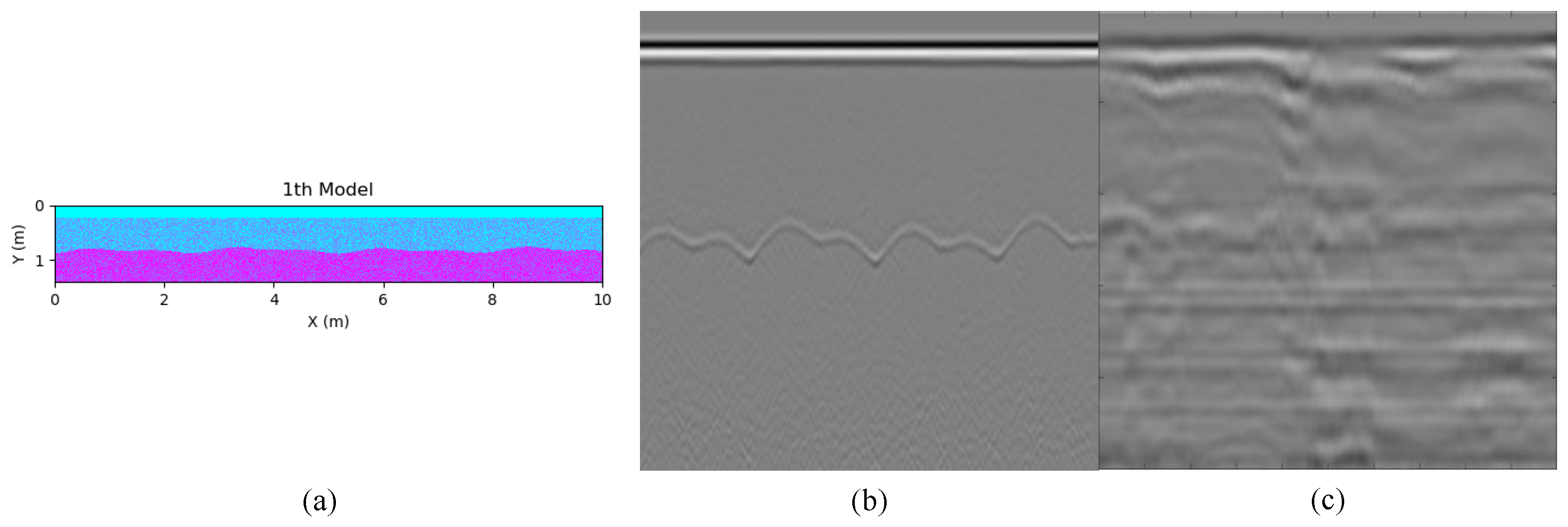
Synthetic data were incorporated into the dataset to address the limited availability of real GPR images of underground tunnel structures. A finite-difference time-domain (FDTD) method was employed to perform forward numerical simulations of secondary tunnel lining structures, generating representative synthetic GPR images to enhance sample diversity in model training. The simulation process was implemented using the open-source electromagnetic wave modeling platform gprMax. The simulation model incorporated the interface structure between primary and secondary lining layers and simulated GPR responses under various thickness conditions, enhancing the model’s adaptability to different structural variations. To increase the realism of the simulated data and better approximate actual field acquisition conditions, boundary perturbations and geometric uncertainties were introduced during model construction. These included superimposed interface perturbations based on sinusoidal and piecewise terrain functions, along with Gaussian geometric noise (mean = 0, standard deviation = 0.05–0.1 m) to simulate surface roughness. During signal simulation, additional Gaussian white noise (mean = 0, standard deviation = 8% of maximum amplitude) was added to emulate the environmental and system noise typically encountered in real GPR acquisition. To ensure that the time–frequency characteristics of the simulated data closely match real GPR signals, measured field parameters were referenced throughout the simulation process. The relative permittivity of the secondary lining concrete was set to a mean of 6.3 with a standard deviation of approximately 0.75, while that of the primary lining was set to a mean of 9.7 with a similar deviation. Both materials were assigned a conductivity of 0.001 S/m. The simulation domain was set to 10 m in width and 1.4 m in depth, with a grid resolution of 0.005 m. A Ricker wavelet with a center frequency of 900 MHz was used as the source signal, with the receiving antenna placed 0.1 m away and a time window of 25 ns. The antenna was moved with a step size of 0.01 m, generating a total of 980 B-scan image traces. Perfectly matched layers (PMLs) were applied around the model to suppress boundary reflections and improve simulation accuracy. The introduction of simulated data not only improved the model’s ability to recognize secondary lining structures but also enhanced its generalization across different tunnel scenarios. Figure 1 illustrates the constructed simulation model of the tunnel secondary lining, the synthetic GPR image generated using gprMax, and the corresponding real GPR image.

One of the key challenges in GPR image recognition is the requirement for large-scale datasets to effectively train the network and optimize weight parameters [14]. In contrast to natural photographs, generating meaningful GPR images is more challenging, as it demands additional time and manual effort. A widely adopted solution is transfer learning, which leverages large-scale optical image datasets such as ImageNet or COCO for network pretraining. Pretraining on such datasets can improve convergence during GPR training and enhance recognition accuracy. Transfer learning involves reusing pretrained model parameters obtained from large-scale datasets. These parameters can be embedded into the backbone of the improved model and reused in the target domain. Although the COCO dataset primarily contains natural images with visual features that differ significantly from tunnel radar imagery, low-level statistical features learned from pixel values—such as histograms—can still provide significant benefits in the context of transfer learning [15]. Previous studies have demonstrated that shallow features obtained through transfer learning—such as edges, textures, and geometric patterns—retain strong generalization capabilities in target domains. For example, Dikmen et al. validated the effectiveness of COCO-pretrained models in feature transfer for bridge radar image classification tasks, and noted that even when semantic differences exist between the source and target domains, low-level structural information remains transferable, contributing to faster convergence and improved accuracy in the target task [16].

This study employs model-based transfer learning, where the model is trained on the COCO dataset, and the knowledge gained from the convolutional neural network is transferred to the target domain. Subsequently, a new Neck network and Head network are created, with the transferred network model being integrated into a new convolutional neural network. The pretrained model is then fine-tuned end-to-end using GPR images to update its weights.

The process of transfer learning is illustrated in Figure 2. To ensure the exceptional detection capabilities of the pretrained CNN model, a model pretrained on the COCO dataset is used as the starting point. This dataset encompasses 80 categories and over 200,000 images. After pretraining, the weight parameters of the model’s backbone structure are extracted, and the task model is trained and fine-tuned using the custom radar image dataset. The transfer learning approach is an efficient method that minimizes computational resource requirements, accelerates convergence speed, reduces training time, enhances the training convergence of the GPR dataset, and minimizes the model’s bias in estimating the average thickness of the secondary lining and signal recognition thickness.

3. Tunnel Secondary Lining Recognition and Thickness Estimation Model

This study proposes a tunnel secondary lining recognition and thickness estimation model based on the YOLOv8-seg framework, leveraging the feature extraction capability of convolutional neural networks and the design of the segmentation head to perform pixel-level segmentation on each detected object, identifying the secondary lining area in the input GPR image. Figure 3 illustrates the deep learning model framework used for recognizing the tunnel secondary lining.

The backbone network of the model is composed of standard convolution layers (Conv), the C2f module with cross stage partial connections (CSPs) [17], and spatial pyramid pooling fast (SPPF). The backbone network extracts the features of the in-phase axis wave groups associated with the tunnel lining layers in GPR images. The lower layers of the network primarily capture low-level features, such as edges and colors of the in-phase axis wave groups. The network subsequently extracts more complex texture features, followed by the detection of more complete contour and shape features of the in-phase axis wave groups, which possess distinguishable identifying elements.

The feature fusion network, Neck, utilizes the feature pyramid network (FPN) [18] architecture for top–down sampling, transferring high-level semantic features downward to ensure that the lower-level feature maps contain richer tunnel lining features. Additionally, the path aggregation network (PAN) [19] structure is employed for bottom-up sampling, transmitting strong localization features from lower layers upwards to enhance the precise localization information in higher-level feature maps. The parameters are aggregated from different backbone layers to different detection layers, enhancing the representation of multi-scale features.

The Head network employs a Decoupled-Head detection head to divide the input feature layers of varying sizes into three branches for detection. The first branch performs a regression task after convolution, outputting a bounding box prediction for the tunnel secondary lining’s location. The second branch performs a classification task after convolution, outputting the probabilities of the classes. The third branch performs a segmentation task after convolution, outputting a feature map used as the Mask coefficients. Additionally, a feature map of scale 52 × 52 is upsampled and output as the native segmentation feature map. By combining it with the Mask coefficients, the tunnel secondary lining segmentation result can be obtained after cropping and binarization.

To improve the accuracy of secondary lining recognition in GPR images, we integrate the Convolutional Block Attention Module (CBAM) [20] into the YOLOv8-seg architecture. Specifically, a novel CBAM-Bottleneck module is constructed by embedding CBAM into the Bottleneck component, which is then integrated into the standard C2f module to form the enhanced C2fCBAM structure. In the revised architecture, the final three C2f modules in the Neck are replaced with C2fCBAM modules, enabling the attention-guided feature fusion of GPR images. This attention mechanism guides the model to focus more effectively on the two primary reflection horizons in GPR images by leveraging both channel and spatial attention pathways, thereby improving overall segmentation performance.

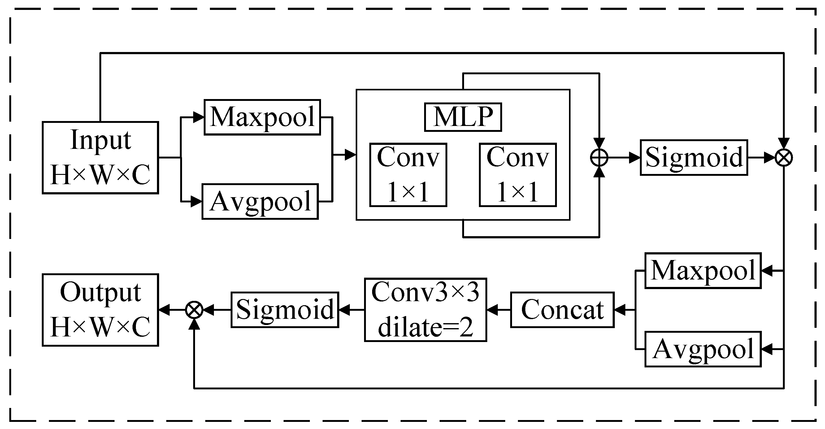
CBAM is a lightweight attention mechanism designed for seamless integration into convolutional neural networks (CNNs), comprising a Channel Attention Module (CAM) and a Spatial Attention Module (SAM) that model the channel importance and spatial relevance, respectively. This method effectively highlights the secondary lining regions of the tunnel, suppresses irrelevant background features, and accentuates the spatial localization of key features within complex backgrounds. The architecture of CBAM is depicted in Figure 4. In contrast to the SE (Squeeze-and-Excitation) module, which models only inter-channel dependencies, CBAM concurrently attends to both channel and spatial dimensions, offering superior adaptability for GPR imaging tasks. Furthermore, CBAM features a compact structure and significantly lower computational overhead compared to recent Transformer-based attention mechanisms, making it more suitable for real-time applications with minimal impact on inference latency. In addition, CBAM has been extensively applied across various image classification and object detection benchmarks, demonstrating significant performance improvements. For instance, in the task of marine debris detection, researchers incorporated CBAM into the YOLOv7 model and compared its performance with lightweight coordinate attention mechanisms and self-attention-based Bottleneck Transformers. The results showed that CBAM outperformed the alternatives, achieving an F1 score of 77% for box detection and 73% for mask evaluation [21]. In a separate study on apple leaf disease detection, researchers combined CBAM with the C3TR module to create the YOLOv5-CBAM-C3TR model, which demonstrated an 8.25% increase in mAP 0.5 compared to the original YOLOv5 model [22]. These findings further confirm that CBAM significantly enhances the model’s ability to focus on target regions.

The CAM module compresses the feature map along the spatial dimension to obtain a one-dimensional vector before further processing. During compression along the spatial dimension, both average pooling and max pooling are considered. Average pooling and max pooling are used to aggregate spatial information from the feature map, which is then fed into a shared network to compress the spatial dimensions of the input feature map. The features are summed element-wise to produce the channel attention map. For a GPR image, channel attention focuses on identifying the regions where the secondary tunnel lining is located. Average pooling provides feedback for each pixel on the feature map, whereas max pooling provides gradient feedback only at the locations with the highest responses during backpropagation. The channel attention mechanism can be expressed as

$$M_c\left(F\right)=\sigma (MLP\left(AvgPool\left(f\right)\right)+MLP\left(MaxPool\left(F\right)\right))$$

(1)

In the equation, the sigmoid activation function is denoted as $\sigma$. The input feature map is first processed through global max pooling and global average pooling, based on width and height, followed by a multi-layer perceptron (MLP) for each. The features output by the MLP undergo element-wise summation followed by a sigmoid activation, resulting in the final channel attention map. The channel attention map is element-wise multiplied with the input feature map to generate the input features required by the spatial attention module.

The SAM module, similar to the CAM module, compresses the channels by applying both average pooling and max pooling along the channel dimension. The MaxPool operation extracts the maximum value along the channel, with the extraction count being the product of height and width. The AvgPool operation extracts the average value along the channel, with the extraction count also being the product of height and width. The feature maps, each with a channel size of 1, are then merged to produce a 2-channel feature map. Through this module, the model is able to focus more effectively on the spatial regions of the tunnel secondary lining, while ignoring background or noise. The spatial attention mechanism can be expressed as

$$M_s\left(F\right)=\sigma \left(f^{7\times 7}[AvgPool\left(F\right);MaxPool\left(F\right)]\right)$$

(2)

In the equation, $\sigma$ denotes the sigmoid activation function, and $f^{7\times 7}$ represents the convolution operation with a kernel size of $7\times 7$.

The improved CBAM-Bottleneck module employs a two-layer convolutional structure during the feature extraction phase, with Figure 5 illustrating both the C2fCBAM module and the proposed CBAM-Bottleneck module in this study. The first convolutional layer compresses the number of channels in the input feature map from c1 to half of the output channels, c2, in order to reduce the computational complexity while retaining key features. The second convolutional layer then restores the channel count back to c2. This provides the foundational features for the subsequent CBAM module. During the channel and spatial attention weighting phase, the convolutional features undergo spatial information extraction via global average pooling and max pooling in the Channel Attention Module, which are then input into an MLP to generate the channel weighting vector. The features pass through the Spatial Attention Module, where global average pooling and max pooling are applied and concatenated, followed by input into the sigmoid activation function to generate the spatial weighting vector, ultimately producing the weighted feature map. The introduction of the attention mechanism further enhances the feature representation capability, allowing the network to more accurately focus on the tunnel secondary lining region, thereby significantly improving the recognition performance for this region.

4. Ablation Study Analysis

The model training in this study was conducted using PyTorch 2.3.0, with the stochastic gradient descent (SGD) optimizer for weight updates. The weight decay was set to 5 × 10⁻⁴, the momentum to 0.937, and the initial learning rate to 1 × 10⁻². To evaluate the impact of transfer learning and the CBAM attention mechanism on model performance, four groups of comparative experiments were designed. Group A used the YOLOv8-seg architecture, which was randomly initialized and trained for 200 epochs on the mixed GPR dataset. Group B adopted the same architecture as Group A, with 100 epochs of pretraining on the COCO dataset followed by 100 epochs of fine-tuning on the mixed GPR dataset. Group C employed the improved architecture with the CBAM attention module, trained from scratch on the mixed GPR dataset for 200 epochs. Group D shared the same architecture as Group C, but its backbone was initialized with pretrained weights from Group B and trained on the mixed GPR dataset for 100 epochs. In terms of computational complexity, the model without CBAM had approximately 110.0 GFLOPs, which slightly increased to 110.2 GFLOPs after CBAM was introduced, indicating minimal overhead. All experiments were conducted on a hardware platform equipped with an NVIDIA RTX 4060 Laptop GPU and an Intel i7-13650HX CPU.

As shown in Figure 6, the recognition results of the four model groups are compared. The first column displays the input GPR images, while the second column visualizes the signal recognition output obtained using the peak amplitude criterion described in [13]. The third to sixth columns show the outputs of Groups A to D, with the secondary tunnel lining regions overlaid in red masks. All input GPR images were generated from 1000 scan traces, corresponding to a maximum two-way travel time of 25 ns. As observed, the output of Group A failed to identify certain secondary lining regions near the image boundaries and mistakenly classified non-lining areas as secondary lining. In Group B, the number of undetected secondary lining regions near the boundaries was noticeably reduced. Similar to Group A, the Group C output also failed to detect some secondary lining regions near the image edges and misclassified some non-lining areas. However, the extent of misclassification was lower than that of Group A. Group D further reduced the number of undetected secondary lining regions near the boundaries.

To estimate the thickness of the secondary lining based on the model’s segmentation output, the relative error of the image-derived thickness was used as a evaluation metric. The image-derived thickness refers to the estimated lining thickness obtained after pixel-level segmentation of the secondary lining region in GPR images using a deep learning model, which is calculated based on the mapping between image pixels and physical distance. The thickness and its relative error were computed using the following equations:

$$H={\displaystyle \frac{C}{\sqrt{\epsilon }}}{\displaystyle \frac{t}{2}}$$

(3)

$$R=\left({\displaystyle \frac{\left|H_{img}-H_{sig}\right|}{H_{sig}}}\right)\times 100\%$$

(4)

where C is the speed of light in vacuum and is set to 0.300 m/ns, $\epsilon$ is the relative permittivity of the medium, and t is the two-way travel time of the electromagnetic wave through the secondary tunnel lining, measured in nanoseconds (ns). The two-way travel time can be converted based on the mapping between the maximum travel time set during field measurements and the image height in pixels. R represents the calculated relative error, $H_{img}$ and $H_{sig}$ refer to the thickness estimated by the image recognition and the thickness obtained using the signal-based recognition method, respectively, both measured in millimeters (mm).

Table 1. Estimated thickness and standard deviation of the secondary tunnel lining.

Track No.	Length (m)	Signal-Based Thickness (mm)	SD of Signal-Based Thickness (mm)	Group A (mm)	SD of A (mm)	Group B (mm)	SD of B (mm)	Group C (mm)	SD of C (mm)	Group D (mm)	SD of D (mm)
1–1000	10	591	44.3	564	88.3	593	62.6	549	89.7	588	31.5
1001–2000	10	558	48.2	679	100.4	595	69.8	512	74.8	544	38.5
2001–3000	10	586	40.8	549	96.6	618	28.8	538	88.6	563	35.2
3001–4000	10	580	43.3	573	98.5	609	37.5	579	82.9	596	32.6
4001–5000	10	592	22.3	589	98.6	611	45.4	587	84.6	614	19.4

lists the secondary lining thickness estimation results of four model groups along Survey Line A in the Longhai tunnel section from D9 + 015.195 to D9 + 065.195. The “Signal-Based Thickness” refers to the signal recognition output obtained using the peak amplitude criterion described earlier.

Table 2. Relative error of image-derived thickness estimation.

Track Number	Group A Restoration Rate	Group B Restoration Rate	Group C Restoration Rate	Group D Restoration Rate
1–1000	4.57%	0.34%	7.11%	0.51%
1001–2000	21.68%	6.63%	8.24%	2.51%
2001–3000	6.31%	5.46%	8.19%	3.92%
3001–4000	1.21%	5.00%	0.17%	2.76%
4001–5000	0.51%	3.21%	0.84%	3.72%
Average Relative Error	6.86%	4.13%	4.91%	2.68%

presents the relative errors between the image-derived thickness and the signal-based thickness.

The IoU values of models A, B, C, and D were 0.779, 0.828, 0.792, and 0.841, respectively. The maximum thickness deviations between the predicted results and the signal-based results were 121 mm, 37 mm, 48 mm, and 23 mm, respectively. With the introduction of the transfer learning strategy, the average relative error between the predicted thickness and the signal-based results was reduced by 2.73%. Based on this, the further integration of the CBAM attention mechanism led to an additional 4.17% reduction compared to the baseline model. In addition, models A, B, and C exhibited significantly higher spatial standard deviations in thickness, possibly due to incomplete identification of secondary lining regions in certain parts of the GPR images. In terms of inference efficiency, the average processing time per image was 27.4 ms and 37.7 ms for models A and B, and 36.7 ms and 28.6 ms for models C and D, respectively. These ablation study results demonstrate that the proposed improved model achieves higher accuracy and stability in recognizing secondary tunnel lining regions, while introducing only a minimal increase in computational cost.

5. Comparative Experimental Analysis

To further evaluate the performance of the improved model, three mainstream instance segmentation models—Mask R-CNN, YOLOv5-seg, and YOLACT—were selected as comparison baselines. Mask R-CNN integrates a Region Proposal Network (RPN) with a Fully Convolutional Network (FCN), offering strong multi-task capability and demonstrating excellent performance in fine-grained segmentation tasks. YOLOv5-seg adds a segmentation head to the YOLOv5 detection framework, enhancing its ability to detect multi-scale object boundaries in complex backgrounds. YOLACT employs a decoupled mask generation mechanism to achieve fast instance segmentation, balancing both object integrity and edge precision. To ensure fairness and consistency in comparison, all three models were pretrained for 100 epochs on the COCO dataset and then fine-tuned for another 100 epochs on the constructed mixed GPR dataset. The specific training settings were as follows: YOLOv5-seg used an initial learning rate of 0.01 with the SGD optimizer, and a linear learning rate decay strategy. Both YOLACT and Mask R-CNN used an initial learning rate of 0.001 with the Adam optimizer and adopted a step-based learning rate adjustment strategy. These configurations ensured a standardized training process and facilitated a fair evaluation of model performance.

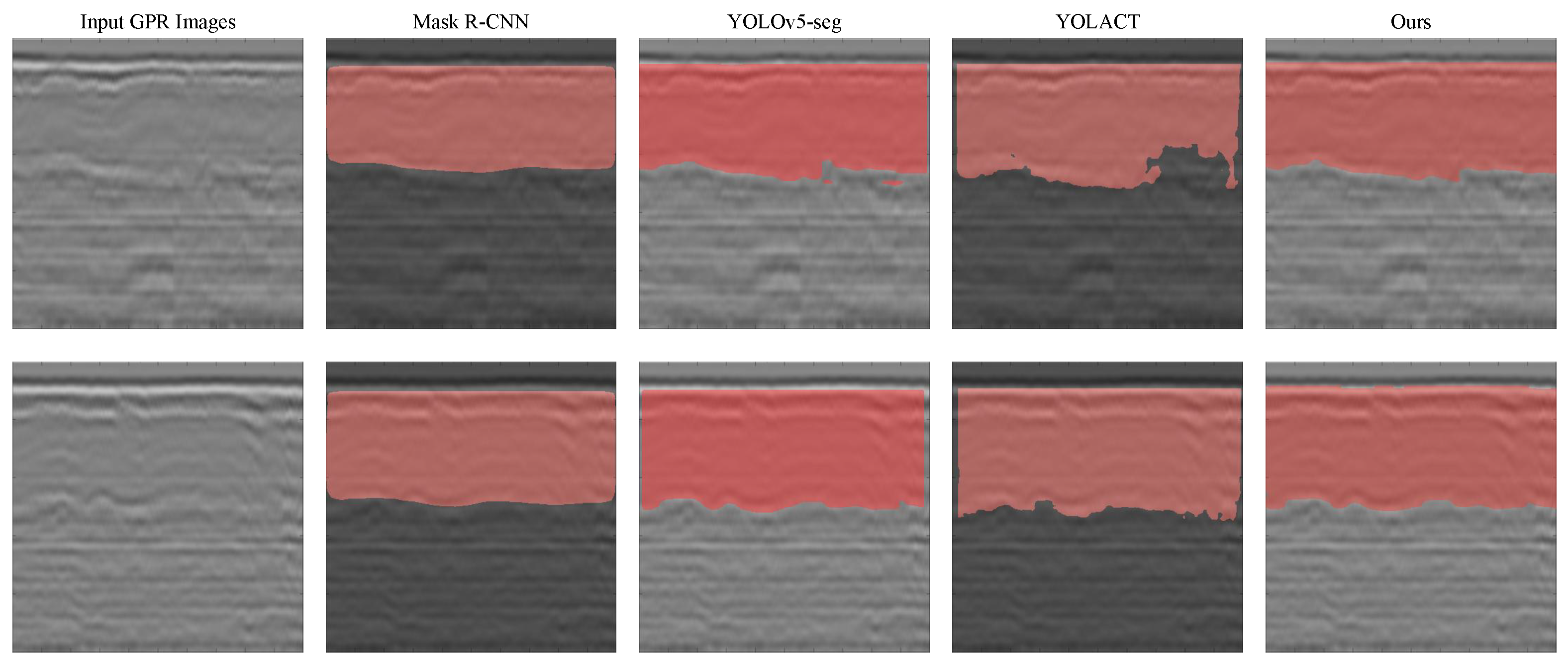
Figure 7 presents a comparison of the experimental results. The first column shows the input GPR images, and the second to fifth columns display the outputs generated by the four models. In the results of YOLOv5-seg and YOLACT, certain secondary lining regions near the image boundaries were not successfully detected. YOLOv5-seg also misclassified some primary lining areas as the secondary lining. Mask R-CNN failed to detect certain secondary lining regions located near the boundary between the secondary and primary linings.

To quantitatively compare the recognition results of the above models, Equations (3) and (4) were used to estimate the image-derived thickness and compute the relative error.

Table 3. Thickness estimation of recognition results from comparison experiment models.

Track No.	Length (m)	Signal-Based Thickness (mm)	SD of Signal-Based Thickness (mm)	Mask R-CNN (mm)	SD of Mask R-CNN (mm)	YOLOv5-seg (mm)	SD of YOLOv5-seg (mm)	YOLACT (mm)	SD of YOLACT (mm)	Improved Model (mm)	SD of Improved Model (mm)
1–1000	10	591	44.3	551	43.2	560	85.2	572	107.3	588	31.5
1001–2000	10	558	48.2	520	35.7	550	20.9	583	90.8	544	38.5
2001–3000	10	586	40.8	521	38.7	548	60.4	541	114.9	563	35.2
3001–4000	10	580	43.3	548	41.1	568	105.1	599	116.7	596	32.6
4001–5000	10	592	22.3	567	37.5	582	102.3	613	104.4	614	19.4

presents the thickness estimation results of the three models.

Table 4. Comparison of experimental models’ thickness estimation and restoration rate of recognition results.

Track Number	Mask R-CNN Restoration Rate	YOLOv5-seg Restoration Rate	YOLACT Restoration Rate	Improved Model Restoration Rate
1–1000	6.77%	5.25%	3.21%	0.51%
1001–2000	6.81%	1.43%	4.48%	2.51%
2001–3000	11.09%	6.48%	7.68%	3.92%
3001–4000	5.52%	2.07%	3.28%	2.76%
4001–5000	4.22%	1.69%	3.55%	3.72%
Average Restoration Rate	6.88%	3.38%	4.44%	2.68%

shows the relative errors between the model-estimated thickness and the signal-based thickness.

The IoU values of the three baseline models were as follows: 0.742 for Mask R-CNN, 0.825 for YOLOv5-seg, and 0.804 for YOLACT. The corresponding maximum thickness deviations from the signal-based results were 65 mm, 38 mm, and 45 mm, respectively. The relative errors were 6.88%, 3.38%, and 4.44%, respectively. In addition, YOLOv5-seg and YOLACT exhibited significantly higher spatial standard deviations in thickness estimation, indicating possible omissions in identifying certain secondary lining regions. By contrast, the proposed improved model achieved a maximum deviation of less than 25 mm from the signal-based results in average secondary lining thickness estimation, with an average relative error of 2.68%, and an IoU value of 0.841, demonstrating superior performance in both thickness estimation accuracy and recognition stability.

6. Conclusions

This study proposes a YOLOv8-seg-based model for secondary tunnel lining recognition and thickness estimation. The model leverages a deep convolutional neural network to perform pixel-level segmentation of secondary lining regions in GPR images and estimate their average thickness. To enhance feature extraction under complex backgrounds, the model incorporates the CBAM attention mechanism, which combines channel and spatial attention to strengthen the response to key interface features. In addition, a transfer learning strategy is applied, where the model is pretrained on the COCO dataset and fine-tuned using both field-measured and numerically simulated data. This approach improves the convergence speed and recognition accuracy under small-sample conditions and enhances the model’s generalization in both architectural design and training strategy. The experimental results demonstrate that the proposed model can reliably identify secondary lining regions in the field dataset collected from the Longhai tunnel. For the section from D9 + 015.195 to D9 + 065.195, the average relative error compared to the signal-based peak detection method was 2.68%. The thickness estimation deviation remained within 25 mm, showing high Intersection over Union (IoU) and low average relative error.

This study still has several limitations. The model relies heavily on representative simulated data and high-quality annotated field data during training, and limitations in data diversity or annotation accuracy may affect its generalization capability. The current model evaluation is limited to a single engineering scenario, and its stability under varying tunnel types, geological conditions, and complex interference environments remains to be validated. In addition, thickness estimation is still based solely on image segmentation, lacking joint modeling with time-domain signals, which may limit prediction accuracy. Future research could expand data sources and integrate raw GPR signals with image information to develop a multimodal model, and incorporate uncertainty estimation mechanisms to enhance model robustness and interpretability in complex scenarios.

References

- Balaguer, C.; Montero, R.; Victores, J.G.; Martínez, S.; Jardón, A. Towards fully automated tunnel inspection: A survey and future trends. In Proceedings of the ISARC—International Symposium on Automation and Robotics in Construction, Sydney, Australia, 9–11 July 2014; IAARC Publications: Montreal, QC, Canada, 2014; Volume 31, p. 1. [Google Scholar]
- Menendez, E.; Victores, J.G.; Montero, R.; Martínez, S.; Balaguer, C. Tunnel structural inspection and assessment using an autonomous robotic system. Autom. Constr. 2018, 87, 117–126. [Google Scholar] [CrossRef]
- Alani, A.M.; Tosti, F. GPR applications in structural detailing of a major tunnel using different frequency antenna systems. Constr. Build. Mater. 2018, 158, 1111–1122. [Google Scholar] [CrossRef]
- Benedetto, A.; Tosti, F.; Ciampoli, L.B.; D’amico, F. An overview of ground-penetrating radar signal processing techniques for road inspections. Signal Process. 2017, 132, 201–209. [Google Scholar] [CrossRef]
- Qin, H.; Zhang, D.; Tang, Y.; Wang, Y. Automatic recognition of tunnel lining elements from GPR images using deep convolutional networks with data augmentation. Autom. Constr. 2021, 130, 103830. [Google Scholar] [CrossRef]
- Li, X.; Liu, H.; Zhou, F.; Chen, Z.; Giannakis, I.; Slob, E. Deep learning–based nondestructive evaluation of reinforcement bars using ground-penetrating radar and electromagnetic induction data. Comput.-Aided Civ. Infrastruct. Eng. 2022, 37, 1834–1853. [Google Scholar] [CrossRef]
- Wang, J.; Zhang, J.; Cohn, A.G.; Wang, Z.; Liu, H.; Kang, W.; Jiang, P.; Zhang, F.; Chen, K.; Guo, W.; et al. Arbitrarily-oriented tunnel lining defects detection from ground penetrating radar images using deep convolutional neural networks. Autom. Constr. 2022, 133, 104044. [Google Scholar] [CrossRef]
- Rosso, M.M.; Marasco, G.; Aiello, S.; Aloisio, A.; Chiaia, B.; Marano, G.C. Convolutional networks and transformers for intelligent road tunnel investigations. Comput. Struct. 2023, 275, 106918. [Google Scholar] [CrossRef]
- Huang, J.; Yang, X.; Zhou, F.; Li, X.; Zhou, B.; Lu, S.; Ivashov, S.; Giannakis, I.; Kong, F.; Slob, E. A deep learning framework based on improved self-supervised learning for ground-penetrating radar tunnel lining inspection. Comput.-Aided Civ. Infrastruct. Eng. 2024, 39, 814–833. [Google Scholar] [CrossRef]
- Liu, B.; Zhang, J.; Lei, M.; Yang, S.; Wang, Z. Simultaneous tunnel defects and lining thickness identification based on multi-tasks deep neural network from ground penetrating radar images. Autom. Constr. 2023, 145, 104633. [Google Scholar] [CrossRef]
- Yue, Y.; Liu, H.; Lin, C.; Meng, X.; Liu, C.; Zhang, X.; Cui, J.; Du, Y. Automatic recognition of defects behind railway tunnel linings in GPR images using transfer learning. Measurement 2024, 224, 113903. [Google Scholar] [CrossRef]
- Zhao, L.; Xu, Q.; Song, Z.; Meng, S.; Liu, S. Dynamic wave tunnel lining GPR images multi-disease detection method based on deep learning. NDT E Int. 2024, 144, 103087. [Google Scholar] [CrossRef]
- Li, C.; Li, M.J.; Zhao, Y.G.; Liu, H.; Wan, Z.; Xu, J.C.; Xu, X.P.; Chen, Y.; Wang, B. Layer recognition and thickness evaluation of tunnel lining based on ground penetrating radar measurements. J. Appl. Geophys. 2011, 73, 45–48. [Google Scholar] [CrossRef]
- Ozkaya, U.; Melgani, F.; Bejiga, M.B.; Seyfi, L.; Donelli, M. GPR B scan image analysis with deep learning methods. Measurement 2020, 165, 107770. [Google Scholar] [CrossRef]
- Neyshabur, B.; Sedghi, H.; Zhang, C. What is being transferred in transfer learning? Adv. Neural Inf. Process. Syst. 2020, 33, 512–523. [Google Scholar]
- Dikmen, M. Investigating Transfer Learning Performances of Deep Learning Models for Classification of GPR B-Scan Images. Trait. Signal 2022, 39, 1761–1766. [Google Scholar] [CrossRef]
- Wang, C.Y.; Liao, H.Y.M.; Wu, Y.H.; Chen, P.Y.; Hsieh, J.W.; Yeh, I.H. CSPNet: A new backbone that can enhance learning capability of CNN. In Proceedings of the IEEE/CVF Conference on Computer Vision and Pattern Recognition Workshops, Seattle, WA, USA, 14–19 June 2020; pp. 390–391. [Google Scholar]
- Lin, T.Y.; Dollár, P.; Girshick, R.; He, K.; Hariharan, B.; Belongie, S. Feature pyramid networks for object detection. In Proceedings of the IEEE Conference on Computer Vision and Pattern Recognition, Honolulu, HI, USA, 21–26 July 2017; pp. 2117–2125. [Google Scholar]
- Liu, S.; Qi, L.; Qin, H.; Shi, J.; Jia, J. Path aggregation network for instance segmentation. In Proceedings of the IEEE Conference on Computer Vision and Pattern Recognition, Salt Lake City, UT, USA, 18–23 June 2018; pp. 8759–8768. [Google Scholar]
- Woo, S.; Park, J.; Lee, J.Y.; Kweon, I.S. Cbam: Convolutional block attention module. In Proceedings of the European Conference on Computer Vision (ECCV), Munich, Germany, 8–14 September 2018; pp. 3–19. [Google Scholar]
- Lv, M.; Su, W.H. YOLOV5-CBAM-C3TR: An optimized model based on transformer module and attention mechanism for apple leaf disease detection. Front. Plant Sci. 2024, 14, 1323301. [Google Scholar] [CrossRef] [PubMed]
- Shen, A.; Zhu, Y.; Angelov, P.; Jiang, R. Marine debris detection in satellite surveillance using attention mechanisms. IEEE J. Sel. Top. Appl. Earth Obs. Remote Sens. 2024, 17, 4320–4330. [Google Scholar] [CrossRef]