A Cascade of Encoder–Decoder with Atrous Convolution and Ensemble Deep Convolutional Neural Networks for Tuberculosis Detection

Abstract

Tuberculosis (TB) is the most serious worldwide infectious disease and the leading cause of death among people with HIV. Early diagnosis and prompt treatment can cut off the rising number of TB deaths, and analysis of chest X-rays is a cost-effective method. We describe a deep learning-based cascade algorithm for detecting TB in chest X-rays. Firstly, the lung regions were segregated from other anatomical structures by an encoder–decoder with an atrous separable convolution network—DeepLabv3+ with an XceptionNet backbone, DLabv3+X, and then cropped by a bounding box. Using the cropped lung images, we trained several pre-trained Deep Convolutional Neural Networks (DCNNs) on the images with hyperparameters optimized by a Bayesian algorithm. Different combinations of trained DCNNs were compared, and the combination with the maximum accuracy was retained as the winning combination. The ensemble classifier was designed to predict the presence of TB by fusing DCNNs from the winning combination via weighted averaging. Our lung segmentation was evaluated on three publicly available datasets: it provided better Intercept over Union (IoU) values: 95.1% for Montgomery County (MC), 92.8% for Shenzhen (SZ), and 96.1% for JSRT datasets. For TB prediction, our ensemble classifier produced a better accuracy of 92.7% for the MC dataset and obtained a comparable accuracy of 95.5% for the SZ dataset. Finally, occlusion sensitivity and gradient-weighted class activation maps (Grad-CAM) were generated to indicate the most influential regions for the prediction of TB and to localize TB manifestations.

1. Introduction

Infectious diseases are major threats to global health, and TB is the world’s top infectious killer and also the major cause of death among people with HIV/AIDS. It is caused by the Mycobacterium tuberculosis bacterium that attacks the lungs. TB spreads when a person, with active TB, coughs, sneezes, or otherwise expels the bacteria. In its 2019 TB report, the WHO estimated that 10 million people were ill with TB (5.7 million males, 3.2 million females, and 1.1 million children) in 2018. Even though it is preventable and curable, it claimed 1.5 million deaths in 2018 [1] and kills over 4000 people each day. TB occurs all over the world, whereas over 95% of cases and deaths are in middle- and low-income countries. The WHO reported that geographically high TB burden countries are in the Southeast Asian region, with 44% of new cases, followed by the African region, with 24% of new cases, and the Western Pacific with 18%, in 2018. People with HIV have a 15–22% higher risk of contracting tuberculosis than those without HIV. Undernourished people are also at high risk because their immune systems are impaired. Thus, developing countries, with widespread poverty and undernutrition, are the most TB-prevalent regions. A rising number of multi-drug-resistant bacteria has exacerbated the TB burden. Thus, TB remains a key factor in public health and a health security threat [1]. Despite increases in notifications, there are still many undiagnosed cases because people with TB are not being checked. Early diagnosis and prompt treatment are crucial to reducing TB-related deaths and curtailing their onward transmission, allowing us to end TB epidemics.

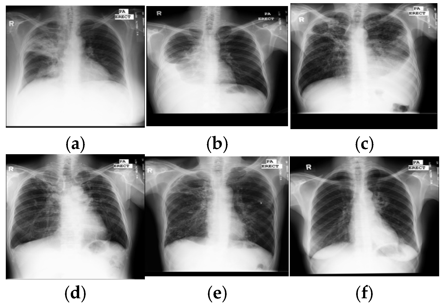
With rapid molecular analysis and bacteria culture methods, TB detection is now very accurate [2]. However, their limited availability and expense restrict widespread use in under-resourced countries with a high TB burden. Because they are not expensive and easily accessed, chest X-rays are mandatory for every evaluation of TB and become a critical screening, diagnostic, and triaging tool for TB and other lung diseases, including lung cancer, pneumonia, etc. A chest X-ray covers all thorax anatomical structures and is a high-yield test at a low cost from a single source. Common manifestations of TB, in X-ray images, are infiltrations, cavitations, consolidations, pleural effusion and thickening, opacities, miliary pattern, and nodules. Some typical TB lesions are shown in Figure 1. More examples of TB manifestations can be found in Daley et al.’s primer [3].

Diagnosis of TB in X-rays is still limited in under-resourced countries where sufficient trained experts to interpret every radiograph are not available. Moreover, TB manifestations are complex and diverse, so manual detection is difficult, even for radiologists. Further, TB lesions that overlap with other disease lesions can imitate many other lung diseases. These discrepancies cause significant observer variation in TB detection. Fortunately, with the advent of digital X-rays and advanced computer vision techniques, computer-aided diagnosis has become an alternative to the expert reading of radiographs. It is hoped that an inexpensive and accurate TB detection algorithm can make the widespread screening of TB a reality in large populations with limited medical resources and alleviate human observer errors.

Reported methods for automatic interpretation of TB range from conventional machine learning methods [4,5,6,7,8,9,10,11,12,13,14] to deep learning methods [15,16,17,18,19,20]. Intuitively, interpretation pipelines have two steps: segmentation of the lung region and prediction of TB manifestations. Lung regions were mostly segmented by a lung atlas-driven method, and then the TB was predicted based on hand-crafted features, followed by a supervised classifier or deep learning method, or a hybrid of both. Typical hand-crafted features were shapes and textural features. Ginneken et al. [4] used multi-scale feature banks for feature extraction, followed by a weighted nearest-neighbor classifier; they achieved an area under the receiver operating characteristic curve (AUC) of 98.6% and 82% on two private datasets. Hogeweg et al. [5] proposed an algorithm to detect the textural abnormality at the pixel level for TB diagnosis. The algorithm provided AUCs between 67% and 86%. Tan et al. [6] segmented lung regions using a user-guided snake algorithm, used first-order statistical features, and a decision tree classifier to classify between normal and X-rays showing TB. On a small custom dataset, their highest accuracy was 94.9%. Unfortunately, those studies were hampered by a lack of publicly accessible datasets for comparison.

In 2014, Jaeger et al. made two datasets publicly available—SZ with 662 images and MC with 138 images [21]. These datasets led to an increased focus on automated TB detection in X-ray images. Jaeger et al. first segmented the lung region, using optimized graph cut methods, then extracted two sets of different features: object detection-inspired features and content retrieval ones. Finally, those extracted features were fed to the support vector machine (SVM) classifier to classify either negative or positive TB and obtained AUCs of 86.9% for MC and 90% for SZ datasets [7]. Vajda et al. [8] sequentially combined the atlas-driven lung segmentation, the extraction of the multi-level features of shape, curvature and eigenvalues of the Hessian matrix, the wrapper feature selection, and a multi-layer perceptron (MLP) network and obtained promising results with AUCs of 87% for MC and 99% for SZ. A combination of shape and texture features was studied by Karargyris et al. [9], who used an atlas-based method for lung segmentation and SVM as a classifier. The authors obtained an AUC of 93.4% for the SZ dataset. Jemal [10] used another texture feature-based method; after segmenting the lung region by thresholding, he extracted the textural features and, finally, differentiated between positive and negative using SVM and achieved AUCs of 71% for MC and 91% for SZ. Santosh and Antani [11] used multi-scale features of shape, edge, and texture, and a combination of a Bayes network, MLP, and random forest to discriminate between negative and positive, yielding AUCs of 90% for MC and 96% for SZ. The multiple instance learning methods [12] used moments of pixel intensities as features and SVM as a classifier and led to AUCs between 86% and 91% for three private datasets. In addition, the prediction scores were used to indicate the diseased regions using heat maps.

Recently, DCNNs were used for TB detection. They were based on the networks trained on ImageNet. Hwang et al. [13] first used the pre-trained AlexNet for the detection of TB and achieved AUCs of 88.4% for MC and 92.6% for SZ datasets. A variant of AlexNet architecture, with a depth of five convolutional blocks and additional skip connections, was presented by Pasa et al. [14] to obtain AUCs of 81.1% (MC) and 90% (SZ). They also generated the saliency maps and Grad-CAM to visualize the disease regions. Lopes et al. [15] analyzed three ways to use the pre-trained networks as the feature extractor. Features from GoogleNet, ResNet, and VGGNet were analyzed along with an SVM classifier—the highest AUC was 92.6% for both MC and SZ datasets.

However, an individual DCNN sometimes produces unsatisfactory results due to limited hypothesis space or descent into local minima. Ensembles of DCNN models have been reported to provide better accuracy than individual DCNNs. Islam et al. [16] combined Alexnet, VGG16, VGG19, ResNet18, ResNet50, and ResNet152 CNN models and achieved a 94% AUC for the SZ dataset. Similarly, AlexNet and GoogLeNet were combined by Lakhani and Sundaram [17], evaluated on four different datasets with 1007 images, and they achieved an AUC of 99%. Rajaraman et al. [18] first segmented the lung region using the atlas-based method, then built a stacked model of hand-crafted features and deep DCNNs; they reported AUCs for four datasets: MC 98.6% and SZ 99.4% and two additional datasets that they built—Kenya 82.9% and India 99.5%.

To date, lung segmentation in TB detection has mainly been based on the lung atlas-driven method and thresholding. Despite the superior performance of deep semantic segmentation in medical image segmentation [19,20,22], these methods have not been applied to lung segmentation in the TB detection framework. To fill this gap, we studied and evaluated a set of deep semantic models for lung segmentation and compared their performance. For TB prediction, a few machine learning-based methods [8,11] performed on par with DCNNs. However, their composite frameworks are more complex than that of an end-to-end DCNN and require more development work. Previous studies showed that ensembles of DCNNs were more efficient than individual ones [16,17,18] and attained state-of-the-art results [18]. Although those ensemble methods achieved promising results, their ensembles only included a limited number of DCNN architectures and did not explore other potential models. Therefore, we herein present an alternative ensemble method of DCNNs, where several DCNN models were used as candidate learners. We noted that, currently, (a) combining all DCNNs can lead to excessive computation times, and (b) a poor choice of DCNN models for fusion can result in poor performance; thus, different combinations of twelve DCNNs were established and evaluated for accuracy, based on several trial runs. After the trial runs, the combination providing the maximum accuracy was selected as a final ensemble classifier.

Moreover, although DCNN-based models have achieved promising results in TB diagnosis, there are few studies on the visualization and interpretation of CNNs. The success of DCNNs, coupled with a lack of interpretable decision-making, raises an issue of trust. Especially in medical diagnosis, lack of interpretability is not acceptable, since a poorly interpreted model’s behavior could adversely affect decision-making. Recently, research has shown that DCNNs are able to locate objects to highlight the indicative features to support decision-making and allow visualization in the form of heat maps. 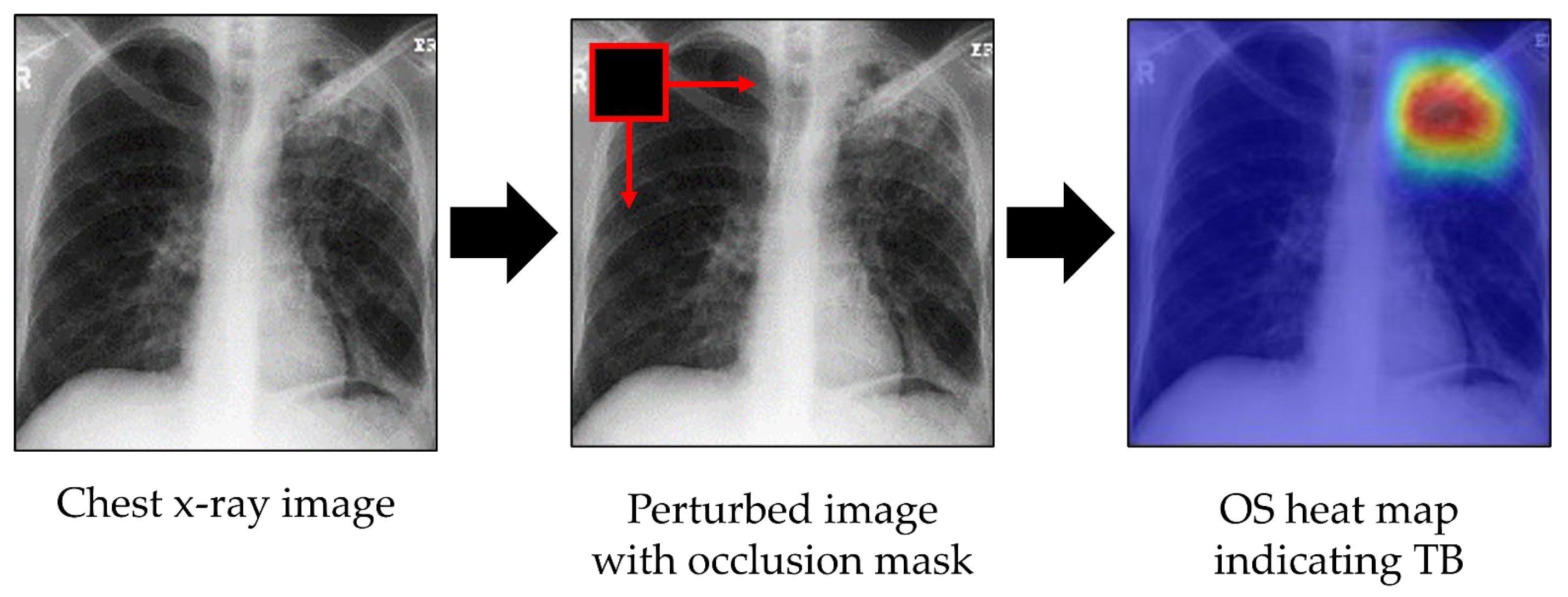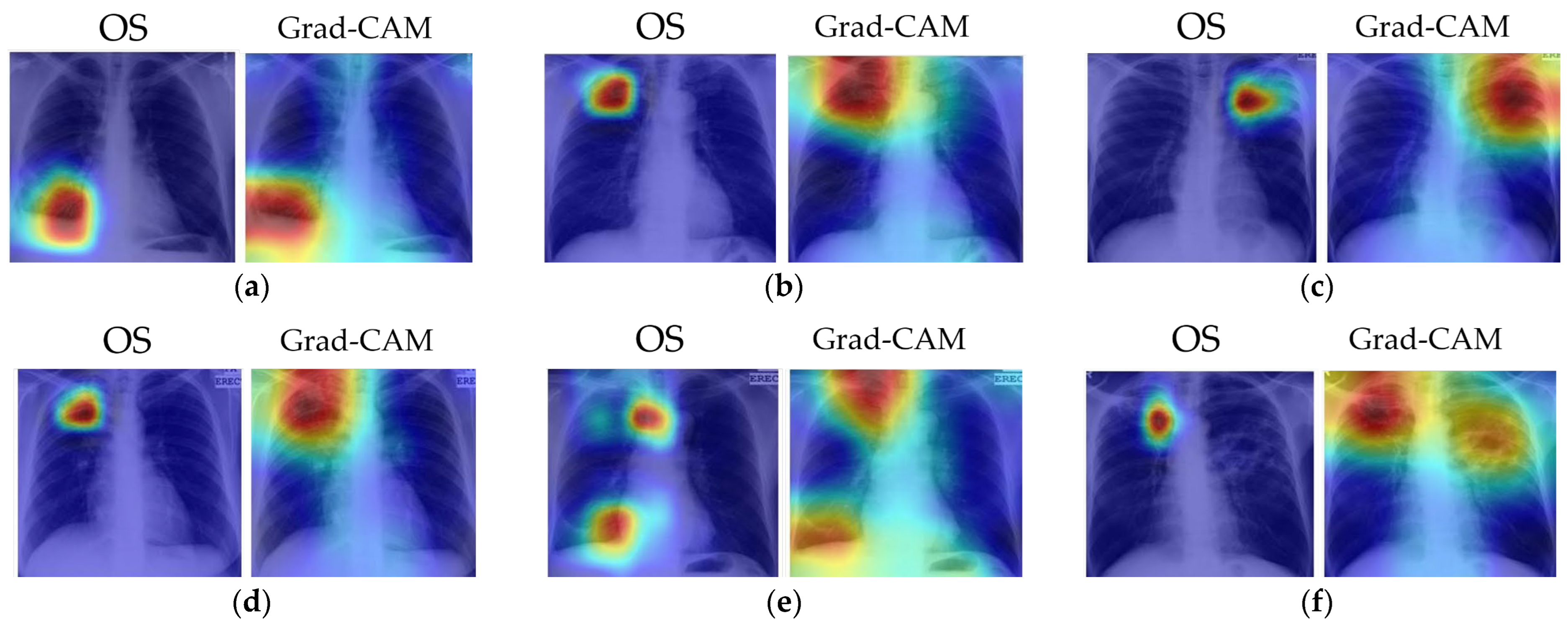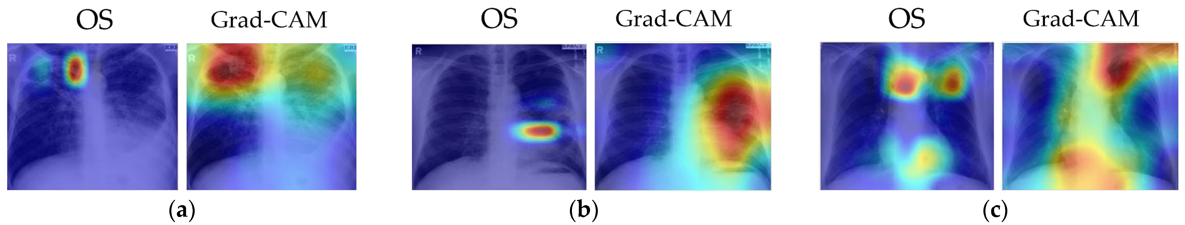Many techniques were introduced to visualize, interpret, and explain the learning process of DCNNs [23,24,25,26]. Here, we visualized DCNN decision-making (i) to identify the indicative features and regions in images for TB prediction and (ii) to localize the lesions using occlusion sensitivity [25] and Grad-CAM heat maps [26].

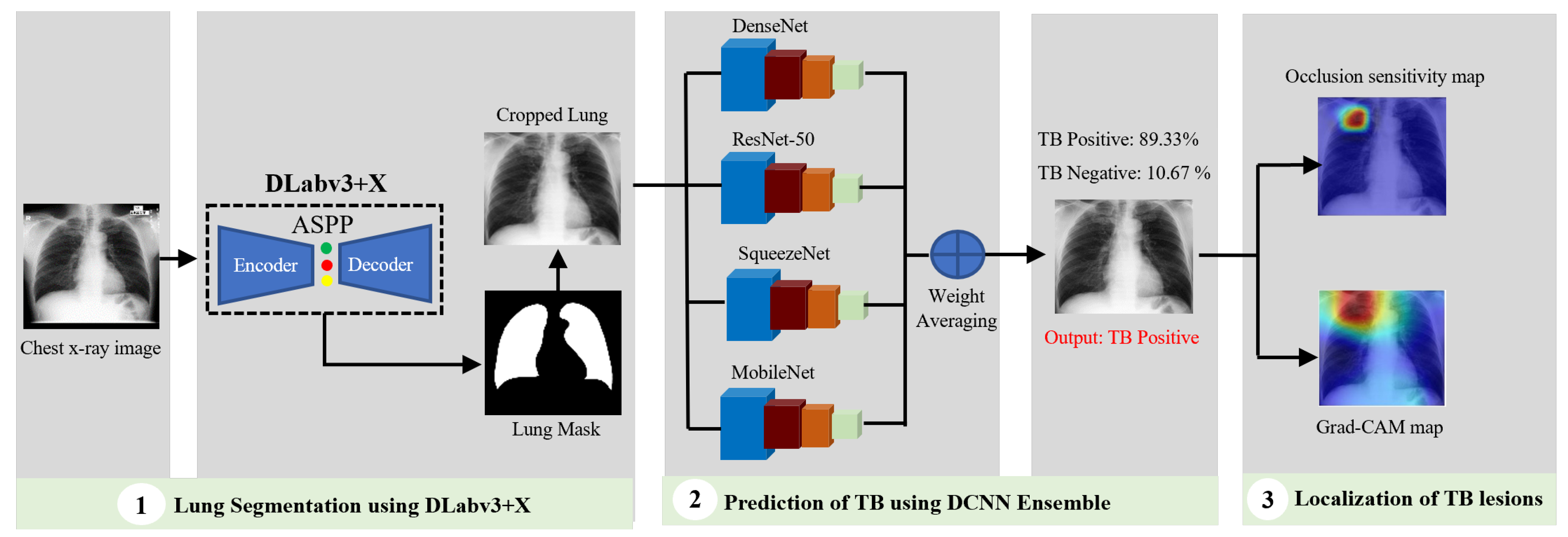
In summary, we present an algorithm for TB detection and localization of its manifestations in images by cascading the DLabv3+X semantic segmentation algorithm and the ensemble of DCNNs, followed by visualization and localization. There are three main contributions:

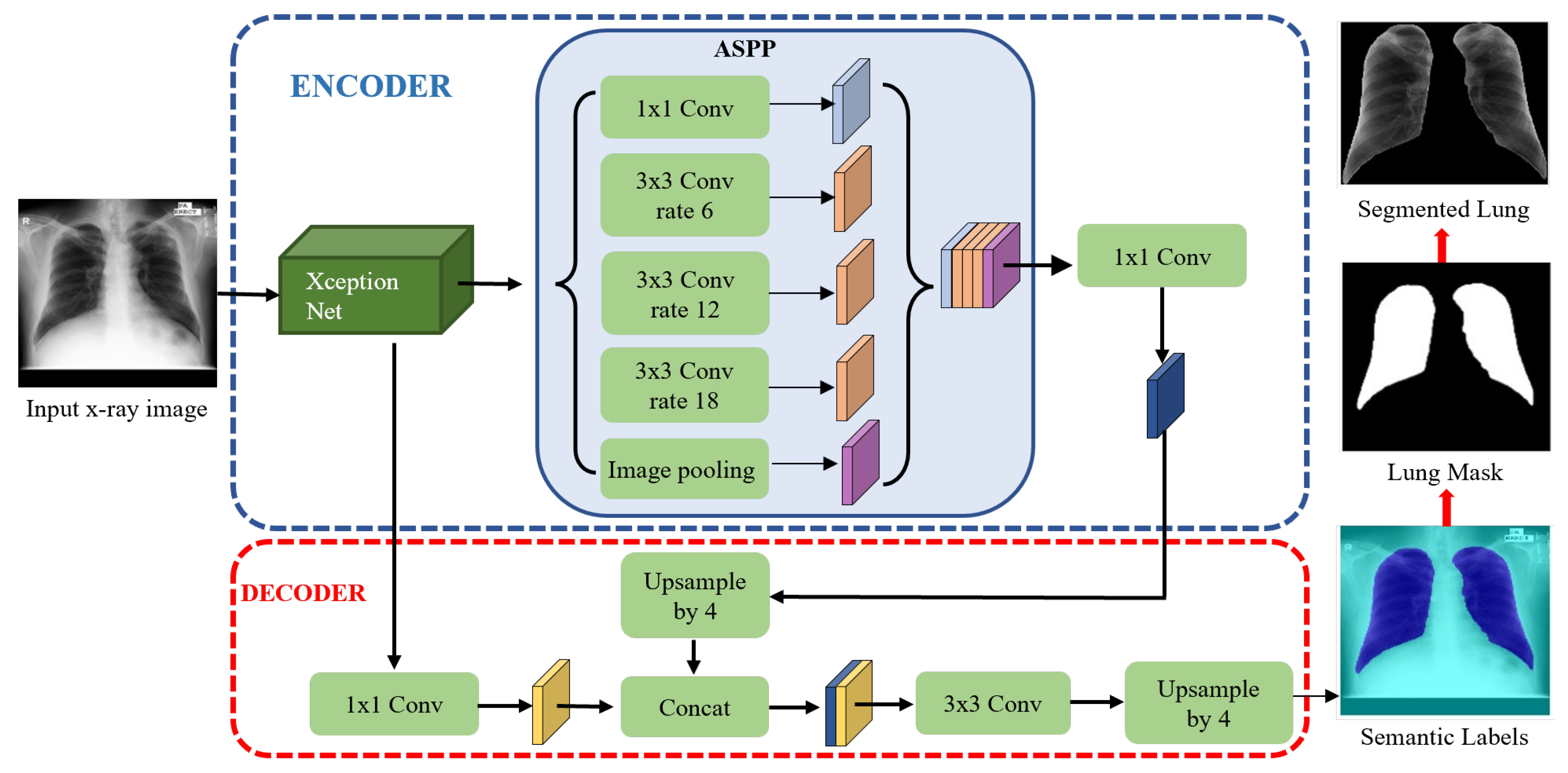
• A novel lung segmentation algorithm using DLabv3+X and comparing it with other deep learning-based methods. Although semantic segmentation algorithms have been applied in lung segmentation, most of them were evaluated using datasets with no TB manifestations. Therefore, we provide a comprehensive comparison of deep semantic algorithms for lung segmentation in the presence of TB lesions.
• Finding the best combination of DCNN models to build the ensemble classifier.
• Identifying features and regions that indicate the presence of TB and localizing the lesions using OS and Grad-CAM.

In the following sections, Section 2 presents the datasets used in the experiments, and Section 3 describes our methodology. The results and discussion of them follow in Section 4. The limitations and future directions are described in Section 5. We conclude in Section 6.

2. Dataset

Our experiments used two main public datasets of chest X-ray images provided by the National Library of Medicine [21]. Images in the MC dataset were collected under the TB control program of the Department of Health and Human Services of Montgomery County, MD, USA: it includes the ground-truth TB labels, clinical reports, along with the location of TB lesions and manually generated lung segmentation masks. The SZ images were collected from the Shenzhen No. 3 Hospital, Shenzhen, China; they include the ground-truth labels but do not include clinical reports or segmentation masks.

Table 1. Brief description of the datasets.

Dataset	Non-TB	TB	File Type	Image Resolution (Pixels)
MC	80	58	PNG	4892 × 4020 or 4020 × 4892
SZ	326	336	PNG	948–3001 × 1130–3001

briefly describes the datasets used: they were fully described by Jaeger et al. [21].

3. Methodology

In conventional tuberculosis (TB) detection using chest X-ray images, the workflow is typically divided into two main stages: lung segmentation and TB manifestation prediction. Based on an extensive review of prior research, DLabv3+X has been identified as an effective technique for segmentation tasks, while an ensemble of Deep Convolutional Neural Networks (DCNNs), which integrates multiple neural network models, demonstrates superior predictive performance compared to individual models. Therefore, our algorithm used a cascade of DLabv3+X lung segmentation and an ensemble of DCNNs for TB diagnosis and localization. It has three main branches: lung segmentation, prediction of TB, and visualization and localization of TB lesions. A DLabv3+X-based segmentation branch was used as the basis for normalization and extraction of lung regions from the background. The DCNN ensemble branch aimed to predict the presence of TB and make a diagnosis decision. The visualization branch showed the location of possible diseased areas. A schematic diagram of our cascade algorithm is in Figure 2.

3.1. Lung Segmentation Using DLabv3+X

Segmentation is an essential prerequisite for medical image analysis: it delineates regions of interest and isolates them from irrelevant regions. In our application, segmentation segregates the lung regions from the other parts of chest X-rays since manifestations of TB appear there. Lung segmentation is also useful for the detection of other thorax diseases. Extensive previous work on lung segmentation or lung boundary detection falls into five groups: (1) rule-based methods, (2) pixel classification methods, (3) deformable-based methods, (4) hybrid methods, and (5) deep learning-based methods [27,28,29,30,31,32,33,34,35,36,37,38,39,40,41]. Rule-based methods establish sequential and heuristic rules to detect the lung regions; they are usually used in initial steps toward more effective segmentation [29,30]. Pixel classification methods train a classifier on a training dataset containing images and ground truth masks. Then, the trained classifier assigns each pixel a lung or a non-lung label [31,32]. Deformable methods use both low-level appearance and shape priors of the lung. The well-known deformable methods are active appearance models and active shape models, in which the shapes of the lung in the training images are modeled, and then the shape model is iteratively deformed to fit the test images [33,34,35]. In hybrid methods, the best portions of the techniques were blended for a better segmentation approach [36,37,38]. In a deep learning-based approach, the deep convolutional layers automatically learn a hierarchy of low-level to more abstract features to classify image pixels. Recently, a number of architectures for deep semantic segmentation have been reported, e.g., fully convolutional network (FCN) [42], U-Net [43], SegNet [44], and the DeepLab series [45,46,47]. FCN, SegNet, U-Net, and atrous convolution-based deep semantic segmentation were used to constrain the lung region for lung nodule detection [39,40,41].

Although the DeepLab series has been frequently used for image segmentation, no use for lung segmentation has been reported, especially for TB diagnosis. In the DeepLab series, DeepLabV3+ [47], a modified variant, based on spatial pyramid pooling (SPP), achieved state-of-the-art results for the PASCAL VOC 2012 and Cityscapes datasets. It combined the advantages of SPP networks and encoder–decoder networks, in which SPP networks are able to encode rich semantic information with different receptive views, and encoder–decoder networks are able to extract detailed information on object boundaries well [45,46,47]. Motivated by its performance and inspired by the ideas of flexibility and efficiency of information flows, DeepLabv3+ with XceptionNet [48] backbone: DLabv3+X, was adopted to segment the lung region here. Before feeding images into the segmentation phase, they were resized to a common 512 × 512 resolution to lower computation time.

The DLabv3+X lung segmentation schematic, formed from an encoder and a decoder, is in Figure 3. In the encoder, XceptionNet was used as a backbone network to retrieve the dense feature maps, with detailed semantic information. After feature extraction, Atrous Spatial Pyramid Pooling (ASPP) at multiple scales, found the rich information. In the ASPP segment, atrous separable convolution with four different rates was applied on the last layer of XceptionNet to retrieve a wider view of the image features. The extracted feature maps from different receptive fields were then concatenated using SPP. Then, 1 × 1 convolution extracted the best higher semantic features from the encoder and reduced the number of channels.

In the decoder module, the encoder features from ASPP, which encodes the rich semantic information, were first bilinearly upsampled by a factor of four and then aggregated with the respective low-level features from XceptionNet, which encoded the details of the object boundaries. Since the low-level features hold a great number of channels which may dominate the influence of the rich encoder features, 1 × 1 convolution is used to lessen the number of channels and to speed training before the concatenation. Finally, a 3 × 3 convolution refined the features, and the refined features were bilinearly upsampled by a factor of four. The decoder module generates the semantic mask for lung and non-lung regions. The predicted lung region pixels then form a lung mask, which was superimposed on the original chest X-rays to extract the lung region. A bounding box cropped the region of interest, i.e., all the lung pixels.

3.2. Prediction of TB Using Ensemble of DCNNs

The cropped lung regions from the segmentation branch were input into the prediction branch, which classified negative or positive TB. The cropped images were again resized to 512 × 512 pixels and enhanced with contrast-limited adaptive histogram equalization (CLAHE) [49]. The prediction stage was based on DCNN. A DCNN scans over an image using the convolutional filters to extract the local features and aggregates these features to generate a prediction for the whole image. DCNNs automatically learn their parameters from a multitude of images labeled with the ground truths using an iterative updating of the parameters to minimize the prediction error, computed by comparing the DCNN prediction against the ground truth. The resulting DCNN can generate predictions on previously unseen images from the testing dataset.

Twelve DCNN models: AlexNet [50], GoogleNet [51], Inceptionv3 [52], ResNet-50, ResNet-101 [53], VGG-16, VGG-19 [54], XceptionNet [48], SqueezeNet [55], ShuffleNet [56], MobileNet [57], and Densenet [58], trained on ImageNet, were used as the pre-trained models. To use the pre-trained DCNNs for TB detection, a new fully connected layer replaced the last fully connected layer of the pre-trained DCNNs. The new fully connected layer was trained on the training dataset of cropped lung images to generate a binary decision indicating the presence or absence of TB. Let X represent an input chest X-ray image, and the output is a binary label y ∈ {0, 1} indicating negative or positive for TB, respectively. For every image in the trained dataset, the weighted binary cross-entropy loss was optimized:

$$CE\left(X,y\right)=\left\{\begin{array}{c}{w}_p\times -\mathit{log}P\left(Y=1/X\right)\hspace{1em}ify=1\\ w_n\times -\mathit{log}P\left(Y=0/X\right)\hspace{1em}ify=0\end{array}\right.$$

(1)

where P(Y = i/X) is the probability that DCNN assigned to the label i, w_p = |N|/(|P| + |N|) and w_n = |P|/(|P| + |N|) where |P| is the number of positive and |N| the number of negative cases in the training dataset.

All DCNN parameters were trained using stochastic gradient descent with momentum (SGDM) [59]. The hyperparameters of training each model with SGDM were optimized using the Bayesian algorithm [60]. Designing an ensemble by combining twelve DCNNs can be time-consuming, and a poor combination of these networks can overfit and result in poor performance. Thus, the optimal combination of DCNNs is defined using trials and errors. Different possible combinations of the trained DCNNs were established by averaging the probability of each DCNN, and the accuracy of each combination is measured. The combination that provided the highest accuracy is retained as the final ensemble classifier. Supposing m is the number of DCNN models and pn is the probability produced for each model, n, the average probability for an ensemble classifier can be computed using (2).

$$averageprobability={\displaystyle \frac{\sum _{n=1}^m{p}_n}{m}}$$

(2)

3.3. Visualization and Localization of TB Manifestations

It is of utmost importance to provide visual explanations for the decision that a deep learning algorithm made. The interpretation and understanding of DCNN is an emerging and active research topic in machine learning, especially for medical diagnosis. A poorly interpreted model could adversely impact the diagnostic decision. To strengthen the user confidence in AI-based models and move towards integrating them into real-time clinical decision-making, we must explain how a DCNN made a decision. Therefore, we added visualization and interpretation to gain insights into the DCNN decision process, evaluate model performance, and localize the TB manifestations. Visualization also helps us to evaluate whether the classification is based on the lesion regions or surrounding areas. Sometimes, the learning algorithm focuses on another part of the chest X-rays rather than TB lesions to make a prediction. Further, it helps to investigate reasons for misclassifications. If the model consistently misclassifies certain types of images, visualization can show the features of the image that are baffling the model. Recently, several researchers have demonstrated progress in the visualization and interpretation of DCNN models [23,24,25,26]. Perturbation techniques and gradient-based class discriminative techniques have been widely used to visualize and understand the behavior of the DCNN models and have made promising achievements. We used two widely used visualization methods: occlusion sensitivity, which implements the perturbation approach [25], and Grad-CAM, which uses gradient-based class discrimination [26].

3.3.1. Occlusion Sensitivity

Occlusion sensitivity (OS) evaluates the sensitivity of the trained model to occlusion. It perturbs different portions of the image with an occlusion mask, typically a gray square mask, and scores the probability of the classification for each perturbed region [25]. Here, the probability score of occlusion of any image region was used to highlight the indicative regions and localize TB lesions. During OS map generation, the occlusion mask was slid through the image, and the probability score of the expected class for each mask was measured. If a region containing TB lesions was occluded, then the classifier should produce a probability lower than a threshold; this falling probability indicates that TB lesions are located in the region of the occlusion. By performing this procedure over the entire image, TB lesions can be detected and localized. Visualization and localization using OS are shown in Figure 4. The colors of the heat map have the following meanings: red = very high lesion, orange = high lesion, yellow = moderate lesion, cyan = low lesion, and blue = no lesion.

3.3.2. Grad-CAM

Grad-CAM is a generalization of class activation maps (CAM). It shows a visual explanation for a decision of all existing DCNN models, whereas CAM itself can only be applied to networks that have a global average pooling layer. The idea behind Grad-CAM is to retrieve the gradient of the prediction probability streaming into the final convolutional layer of a DCNN, import values to each neuron for a decision of a particular task, and indicate the regions of the image that are most significant for classification. The regions with large gradient values are exactly the regions where the prediction score depends mostly on the image. Grad-CAM is applicable to image classification, image captioning, and visual question-answering models [26].

Here, Grad-CAM was used to visualize the indicative regions of images for TB classification and localization of TB manifestations. First, we retrieved the prediction scores, $S_{tb}$, for class $tb$ and the convolutional feature map from the final DCNN layer. $(i,j)$ denotes the ath activation feature map at a location $(i,j)$. Then, the gradient of the prediction score $S_{tb}$ with respect to convolutional feature map $f_a(i,j)$, i.e., $\partial S_{tb}/\partial f_a(i,j)$ was computed. These gradients flowing back were averaged and pooled to obtain the neuron importance ${\beta }_a^{tb}$.

$${\beta }_a^{tb}=\stackrel{glocalaveragepooling}{\overbrace{{\displaystyle \frac{1}{Z}}{\sum }_i{\sum }_j\hspace{1em}\hspace{1em}}}\hspace{1em}\hspace{1em}\underset{gradientsviabackprop}{\underbrace{{\displaystyle \frac{\partial S_{tb}}{\partial f_a(i,j)}}}}$$

(3)

where Z is a constant (the number of pixels in the feature map). The class-discriminative localization map $G{rad-CAM}_{tb}\in {\mathbb{R}}^{i\times j}$ was computed via the weighted sum of all feature maps in the final convolutional layer for the expecting class, tb, after applying the nonlinearity function, ReLU—see (4). ReLU was applied to focus only on pixels that have positive weights for class tb and avoid negative weights from impacting class tb because pixels with negative weights are considered to belong to a non-TB class. ReLU is a widely used activation function in neural networks that avoids the vanishing gradient problem and is computationally faster compared to Sigmoid and Tanh, which require exponential calculations.

$${Grad-CAM}_{tb}(i,j)=RELU\underset{linearcombination}{\underbrace{({\sum }_a{\beta }_a^{tb}{f}_a(i,j))}}$$

(4)

4. Experimental Results and Discussions

The experiments were run in the Matlab 2020a environment on Windows 10 with an NVIDIA T1660Ti GPU and an i7 core.

4.1. Lung Segmentation

The evaluation of lung segmentation was mainly based on the MC and SZ datasets. MC contained manually segmented masks, whereas the ground truth lung masks of the SZ dataset were acquired from Yu et al. [61]. The SZ and MC datasets are randomly partitioned into training and testing in an 80:20 ratio. We used the training dataset for training the algorithm and the testing dataset for evaluating performance. Our DLabv3+X segmentation was a DeepLabv3+ model, where the XceptionNet model was embedded as the backbone network. To show the effectiveness and robustness of XceptionNet as a backbone network, three other networks, ResNet-18, ResNet-50, and MobileNet, were also embedded as the backbone network, labeled DLabv3+R18, DLabv3+R50, and DLabv3+M. All the segmentation models are trained using the Adam optimizer, which is a variant of the stochastic gradient optimization algorithm [62]. We used the default hyperparameters of Adam: an initial learning rate, α = 0.001; decay rate of gradient moving average, β₁ = 0.9; decay rate of squared gradient moving average, β₂ = 0.99. Due to the limitation of GPU memory, the batch size was set to 4. To avoid overfitting in the networks, so that it does not become specific to some patterns in the training set and does not fail to generalize to the testing images, we used early stopping to save the networks after every epoch and to choose the saved network with the minimum loss.

Once the segmentation models were trained, lung segmentation masks for the images were generated for use on the testing dataset. The models’ performance was evaluated at the pixel level by comparing the predicted mask with the ground truth mask. In the literature, different methods have been evaluated with different evaluation metrics [4,5,6,7,8,9,10,11,12,13,14,15,16,17,18]. Here, we judged segmentation method performance using three common metrics: IoU or Jaccard Index, Dice Similarity Coefficient (DSC) score, and average accuracy, computed as

$$PixelAccuracy={\displaystyle \frac{TP+TN}{TP+TN+FP+FN}}$$

(5)

$$IoUorJacardIndex={\displaystyle \frac{\left(GT\bigcap Seg\right)}{\left(GT\bigcup Seg\right)}}={\displaystyle \frac{TP}{TP+FP+FN}}$$

(6)

$$DSC={\displaystyle \frac{2\ast \left|GT\bigcap Seg\right|}{\left|GT\right|+\left|Seg\right|}}={\displaystyle \frac{2TP}{2TP+FP+FN}}$$

(7)

where GT and Seg denote the ground truth mask and the segmented region, respectively. True Positive (TP) refers to lung pixels, which were correctly predicted as the lung. Similarly, True Negative (TN) stands for correctly classified non-lung pixels. On the other hand, False Positive (FP) represents non-lung pixels wrongly segmented as lung, and False Negative (FN) denotes pixels which should have been marked as lung pixels.

Segmentation results for DLabv3+X, along with the alternatives: DLabv3+R18, DLabv3+R50, and DLabv3+M are listed in

Table 2. Performance of deep semantic lung segmentation methods on MC dataset.

Algorithms	IoU (%)	DSC (%)	Accuracy (%)
FCN	86.3 ± 4.2	92.6 ± 2.5	96.2 ± 1.6
Seg-VGG16	89.0 ± 4.0	94.1 ± 2.3	96.8 ± 1.1
Seg-VGG19	87.9 ± 3.3	93.6 ± 1.9	96.5 ± 0.9
U-Net	90.6 ± 5.5	94.9 ± 3.2	97.4 ± 1.4
DLabv3 + R18	94.4 ±1.5	97.1 ± 0.8	98.5 ± 0.3
DLabv3 + R50	93.6 ± 1.6	96.7 ± 0.8	98.3 ± 0.5
DLabv3 + M	92.4 ± 3.2	96.0 ± 1.7	97.9 ± 1.1
DLabv3 + X	95.1 ± 1.5	97.5 ± 0.8	98.7 ± 0.3

for MC and

Table 3. Performance of deep semantic lung segmentation methods on SZ dataset.

Algorithms	IoU (%)	DSC (%)	Accuracy (%)
FCN	85.8 ± 4.2	92.3 ± 2.5	95.9 ± 1.6
Seg-VGG16	86.2 ± 4.0	92.5 ± 2.4	95.9 ± 1.4
Seg-VGG19	85.7 ± 3.7	92.3 ± 2.1	95.7 ± 1.4
U-Net	84.8 ± 9.1	91.5 ± 5.6	95.5 ± 2.6
DLabv3+R18	92.4 ± 4.8	95.9 ± 2.7	97.8 ± 1.7
DLabv3+R50	92.3 ± 4.7	95.9 ± 2.7	97.9 ± 1.6
DLabv3+M	91.8 ± 4.2	95.7 ± 2.4	97.7 ± 1.6
DLabv3+X	92.8 ± 4.2	96.2 ± 2.4	97.9 ± 1.5

for the SZ dataset. The tables show that DLabV3+X segmentation performed better than the other three variants: this is because XceptionNet has the deepest depth among the embed backbone networks. The deeper DCNN model can produce deeper features and covers a wider area in the image, which delivers better segmentation results. Visualizations of DLabv3+X segmentations are in Figure 5.

Even though FCN, SegNet, and U-Net have been used for lung segmentation and provided good results, they were mainly evaluated on the JSRT dataset [63]. Assessing lung segmentation algorithms on this dataset is flawed because the JSRT dataset contains a limited number of lung abnormalities: the only abnormalities found are nodules. The presence of nodules, in most cases, does not affect the lung shape, especially when the nodules are small or are not located in the peripheral lung zone. Therefore, most of the lung regions in the JSRT dataset can be considered normal. On the other hand, the MC and SZ datasets contain a variety of TB manifestations that severely affect the shape and intensity of lung regions. In the severe cases of a cavitary infiltrate, or pleural effusion, the shape and pixel intensity of the lung significantly differ from those of a normal lung. These TB abnormalities can cause problems for segmentation methods, which are modeled on normal lungs only. Therefore, we coded and tested FCN, two variants of SegNet based on VGG16 and VGG17 (labeled Seg-VGG16 and Seg-VGG19), and classical U-Net on the MC and SZ datasets, where many images contain TB pathologies. The same parameter values of our DLabv3+X were used to train these models. Their results are tabulated and compared with DeepLabV3+ based models in Table 2 for MC and Table 3 for SZ. To enable direct comparison with existing studies, we also tested DLabv3+X along with DLabv3+R18, DLabv3+R50, and DLabv3+M on the JSRT dataset. The ground truth masks for the JSRT dataset were obtained from Van Ginneken et al. [28]. Following the same partition ratio of existing studies, the JSRT dataset was split into 50% training and 50% testing. JSRT results are tabulated in

Table 4. Performance of deep semantic lung segmentation methods on JSRT dataset.

Algorithms	IoU (%)	DSC (%)	Accuracy (%)
FCN	83.9 ± 3.9	91.2 ± 2.3	94.8 ± 2.3
Seg-VGG16	87.7 ± 3.6	93.4 ± 2.1	95.7 ± 2.1
Seg-VGG19	86.9 ± 2.6	92.9 ± 1.5	95.5 ± 1.5
U-Net	91.6 ± 3.0	95.6 ± 1.7	97.4 ± 1.7
DLabv3+R18	94.7 ± 2.0	97.3 ± 1.1	98.3 ± 1.1
DLabv3+R50	94.5 ± 1.9	97.1 ± 1.0	98.3 ± 1.0
DLabv3+M	94.9 ± 1.8	97.4 ± 1.0	98.4 ± 1.0
DLabv3+X	96.1 ± 0.8	98.0 ± 0.4	98.8 ± 0.4

. Table 2, Table 3, and Table 4 clearly show that DLabv3+ based models outperformed FCN, SegNet-based methods, and U-Net for all evaluated datasets. Among DLabV3+ based models, our DLabv3+X provided the highest segmentation performance with IoUs of 95.1 ± 1.5% for MC, 92.8 ± 4.2% for SZ, and 96.1±0.8% for JSRT. For the MC dataset, DLabv3+R18 also yielded comparable results to DLabv3+X by giving an IoU of 94.4 ± 1.5%. For the SZ dataset, DLabv3+R18 and DLabv3+R50 obtained the comparable IoUs of 92.4 ± 4.8% and 92.3 ± 4.7% to 92.8 ± 4.2% of DLabv3+X. For the JSRT dataset, DLabv3+R18, DLabv3+R50, and DLabv3+M obtained similar IoUs of 94.7 ± 2.0%, 94.5 ± 1.9, and 94.9 ± 1.8%, respectively, while DLabv3+X achieved the highest IoU of 96.1 ± 0.8%. In

Table 5. DLabv3+ X lung segmentation compared to previous studies.

	Dataset	IoU (%)	DSC (%)	Accuracy (%)
[28]	JSRT	94.6 ± 1.8	-	-
[29]	private dataset	88.0 ±7.0	-	-
[30]	private dataset	80.9	-	-
[31]	JSRT	95.2 ± 1.8	97.5 ± 1.0	-
[32]	JSRT	95.3 ± 2.0	-	-
[33]	JSRT	95.2 ± 1.9	-	-
[34]	JSRT	93.0 ± 1.8	96.4 ±1.0	97.6 ± 0.6
[35]	JSRT	85.4 ± 4.9	-	-
[36]	JSRT	86.9 ± 5.9	-	95.7 ± 2.4
[37]	JSRT	94.5	-	98.2
[38]	JSRT	$95.4\pm$ 1.5	$9.67\pm$ 0.8	-
	MC	$94.1\pm$ 3.4	$96.0\pm$ 1.8	-
[39]	JSRT	95.0	97.4	-
[40]	JSRT + MC	95.1	-	98.7
[41]	JSRT	96.1 ± 1.5	98.0 ± 0.8	-
	MC	93.1 ± 4.9	96.4 ± 2.8	-
Our DLabv3+X	JSRT	96.1 ± 0.8	98.0 ± 0.4	98.8 ± 0.4
	MC	$95.1\pm$ 1.5	$97.4\pm$ 0.8	98.7 ± 0.3
	SZ	92.8 ± 4.2	96.2 ± 2.4	97.9 ± 1.5

, we further compared our segmentation method with extant lung segmentation algorithms and showed that it surpassed existing studies at IoUs 95.1 ± 1.5 for MC and 92.8 ± 4.2 for SZ. For validation, using JSRT, our IoU, at 96.1 ± 0.8, matched Hwang and Park [41], but surpassed others.

4.2. TB Prediction Using Ensemble Model

The MC and SZ datasets were used for the prediction task. All the images were segmented using DLabv3+X and cropped to a bounding box to contain all lung pixels and used as input to the prediction. Twelve DCNNs are trained using the SGDM optimizer with five-fold cross-validation. Due to limited GPU memory, the batch size was set to 4. Since SGDM parameters can strongly affect individual DCNN performance, it is important to select the appropriate values for them. The common parameters for training the DCNN model with SGDM are learning rate, momentum, and L2-regularization’s decay rate. The proper tuning of these parameters can help the DCNN model become more robust and reliable. Therefore, we initially defined the search space: learning rate, α ∈ (0.01, 1), momentum, γ ∈ (0.8, 0.99), and L2-regularization’s decay rate, λ ∈ (0, 1), and searched for optimal values using a Bayesian algorithm. The optimal parameters for each DCNN are listed in

Table 6. Optimal parameters for each DCNN.

Network	Learning Rate (α)	Momentum (γ)	L2-Regularization’s Decay Rate (λ)
AlexNet	1.6 × 10−2	9.0 × 10−1	2.1 × 10−5
GoogleNet	1.1 × 10−2	8.4 × 10−1	3.5 × 10−9
InceptionV3	1.0 × 10−2	8.0 × 10−1	1.5 × 10−10
ResNet-50	1.0 × 10−2	9.0 × 10−1	3.0 × 10−4
ResNet-101	1.3 × 10−2	9.8 × 10−1	1.5 × 10−6
VGG-16	1.0 × 10−2	8.9 × 10−1	1.0 × 10−4
VGG-19	1.0 × 10−2	9.9 × 10−1	2.5 × 10−4
XceptionNet	1.0 × 10−2	8.2 × 10−1	3.6 × 10−10
MobileNet	1.4 × 10−2	9.1 × 10−1	1.0 × 10−4
SqueezeNet	2.1 × 10−1	8.7 × 10−1	9.0 × 10−6
ShuffleNet	2.5 × 10−2	9.1 × 10−1	8.9 × 10−9
DenseNet	1.0 × 10−2	9.5 × 10−1	1.0 × 10−4

. Once each DCNN model learned the optimal parameters, it was combined with the ensemble classifier. Combining all DCNN models consumed large amounts of computation time yet did not improve the overall result, so we attempted to form the best combination of a smaller set of DCNN models. We tested different combinations of trained DCNNs, measured their accuracies, and picked the combination that provided the highest accuracy. The empirical experiments showed that a combination of DenseNet, ResNet-50, SqueezeNet, and MobileNet led to stable and promising results for both datasets. Thus, we built an ensemble classifier of those four DCNNs by averaging their probabilities.

The performance of the ensemble classifier was assessed with three metrics: F-measure (F1), accuracy (ACC), and area under curve (AUC). Using TP, TN, FN, FP, F1, and ACC were computed as

$$F-measure(F1)=2{\displaystyle \frac{Recall\times Precision}{Recall+Precision}}$$

(8)

$$accuracy(ACC)={\displaystyle \frac{TP+TN}{TP+TN+FP+FN}}$$

(9)

where TP is the number of images correctly predicted as TB, TN is the number of correctly predicted normal images, FP is the number of images wrongly predicted as positive for TB, and FN is the wrongly predicted normal images. Recall is TP/TP + FN and precision is TP/TP + FP, respectively. AUC is an important measure for comparing classifiers; it is computed from the receiver operating characteristics curve. Our ensemble classifier results are in

Table 7. Results from individual DCNNs and the ensemble of selected DCNNs (in %).

Algorithms	MC Dataset			SZ Dataset
	F1	ACC	AUC	F1	ACC	AUC
AlexNet	71.2	58.5	72.6	71.9	64.3	78.7
GoogleNet	84.2	85.4	95.2	82.6	83.9	93.3
Inceptionv3	72.7	78.0	93.1	74.8	79.4	92.8
ResNet-50	84.4	82.9	94.3	79.3	81.9	93.8
ResNet-101	68.8	75.6	94.8	78.4	81.4	94.1
VGG-16	68.1	63.4	79.5	65.2	68.8	76.6
VGG-19	66.7	73.2	88.8	59.9	70.4	87.1
XceptionNet	78.9	80.5	92.9	75.6	79.9	94.5
MobileNet	90.5	90.2	96.4	92.9	93.0	98.0
SqueeNet	87.0	85.4	93.6	76.9	80.4	93.0
ShuffleNet	68.8	75.6	95.0	85.7	87.4	96.9
DenseNet	89.5	90.2	97.6	94.2	94.5	99.6
Ensemble	92.7	92.7	99.0	95.3	95.5	99.7

, where they are compared with those for the individual DCNNs. Among individual DCNNs, MobileNet and DenseNet made better predictions than the others. The ensemble of DenseNet, ResNet-50, SqueezeNet, and MobileNet performed better than individual DCNNs. It achieved an accuracy of 92.7 for MC and an accuracy of 95.5 for SZ, significantly better than the accuracy of individual DCNNs.

Table 8. Our cascade algorithm vs. previous studies (in %).

Algorithm	MC Dataset		SZ Dataset
	ACC	AUC	ACC	AUC
Jaeger et al. [7]	78.3	86.9	84.0	90.0
Vajda et al. [8]	78.3	87.0	95.6	99.0
Karargyris et al. [9]	-	-	85.0	93.4
Jemal [10]	68.1	71.0	83.4	91.0
Santosh et al. [11]	83.0	90.0	91.0	96.0
Hwang et al. [13]	67.4	88.4	83.7	92.6
Pasa et al. [14]	79.0	81.1	84.4.	90.0
Lopes et al. [15]	82.6	92.6	84.7	92.6
Islam et al. [16]	-	-	90.0	94
Rajaraman et al. [18]	87.5	98.6	95.9	99.4
Our cascade algorithm	92.7	99.0	95.5	99.7

tabulates the comparison of the prediction performance of the proposed cascade algorithm and the existing studies. The comparison exhibits that the proposed algorithm provides preferable results for both the MC and SZ datasets. It provided significant improvement for the MC dataset. It achieved over 4% better accuracy than previous studies. To our knowledge, our cascade algorithm is the first to achieve over 90% accuracy for the MC dataset.

4.3. Visualization and Localization Result of TB Manifestations

Visualizations and localizations provide a ‘sanity check’, to show where the prediction decisions are made on TB lesions or on the surrounding context of the image, and to assist in validating the model. Since only the MC dataset provides the clinical reports of TB locations, images from the MC dataset only were used to evaluate visualization and disease localization performance.

OS and Grad-CAM methods were used as visualization techniques. OS and grad-CAM heat maps were computed from our method and overlaid on the image to identify the indicative regions of TB manifestation. Intense red pixels show the relevant pixels for a certain class. If the input image was classified as TB positive, intense red pixels label regions, which have a high impact on that decision and indicate the disease location.

To obtain the best results using the OS map, it is vital to use the right side of the occlusion mask and stride options. Tuning their values helps provide more flexibility to investigate the input features at different length scales. From the empirical results, we set the occlusion mask size to 20% of the input square image and the stride to 10% of the input square image. In addition, we used the black occlusion mask containing zero pixel intensity instead of a gray square mask of 128 pixel intensity. This is based on the consideration that the images themselves are primarily the gray level, and occluding using a gray mask does not conceal much information compared to the neighborhood. For Grad-CAM, it required no tuning of any parameters.

Several examples of visual results for the correct TB prediction and lesion localizations are given in Figure 6. It shows that our cascade algorithm correctly detected and localized common TB lesions such as pleural effusion, TB scars, infiltrate, cavity, nodular infiltrate, apical fibrosis lesion, and pleural blunting and infiltrate with calcification. As shown in Figure 7, even though the model correctly predicts TB, it does not always detect all lesions and sometimes counts too many. Frequently, it fails to identify all the lesions when there are multiple lesions. In Figure 7a, both OS and Grad-CAM methods failed to mark a pleural effusion, even though the lesion is significant. In Figure 7b, the algorithm missed locating the lesions in the right lung. Figure 7c shows the over-counting errors. Both OS and Grad-Cam not only detected the TB lesions in the lung region, but also wrongly focused on some regions outside the lung.

The localization maps of OS and Grad Cam differed slightly. Grad-CAM was relatively better in pathologies localization than OS. This could be more obviously noticed when the image presents multiple lesions. The Grad-CAM computation was faster than OS, without needing parameter tuning. However, it commonly provided a lower resolution map than OS and could overlook fine details. Applying object detection networks, e.g., RetinaNet, could allow for explicit localization of TB abnormalities at higher resolutions. However, these networks require the manual annotation of regions of interest or explicit labeling of different TB lesions. Currently, there is no publicly available dataset with the explicit annotation of TB anatomy.

5. Limitations and Future Works

Although our cascade algorithm achieved excellent performance in detecting TB, there are still some limitations in this work and the field in general. The fundamental limitations arise from the datasets, which may limit their clinical applicability or performance in a real-world clinical practice. First, Raoof et al. [64] noted that up to 15% of accurate diagnoses using chest X-rays needed a side or lateral view. Radiologists often use X-rays acquired in both frontal and lateral projections, which aids both disease classification and localization. In this study, we only had available frontal projections, and the lack of lateral views may hinder the detection of some TB manifestations. Future work should use both frontal and lateral chest X-rays, when available, for diagnosis and automated system development. Secondly, clinical information is often necessary for a radiologist to render a specific diagnosis, or at least provide a reasonable differential diagnosis. Due to the lack of sufficient clinical information and pathological findings, our algorithm could not include patient history and other clinical information, which has been shown to improve diagnosis accuracy [65]. Therefore, new datasets, with both frontal and lateral images, clinical reports, and annotated lesions, are urgently needed.

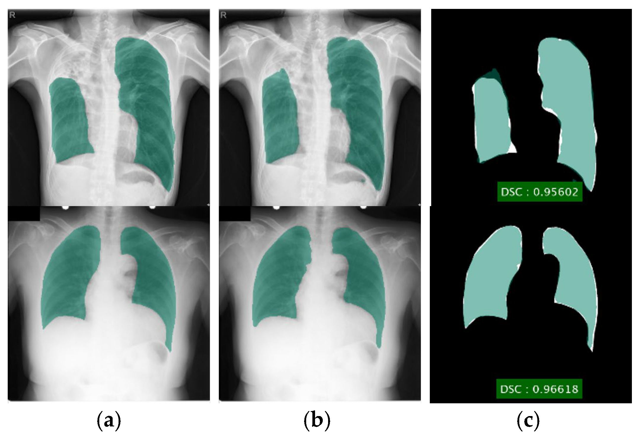
For lung segmentation, images with severe TB manifestations, for instance, severe pleural effusion, resulted in poor segmentation, because pleural effusion regions resemble the background. For these images, our DLabv3+X segmentation method did not generate the correct lung shape, which indicates that the segmentation alone did not capture sufficient intrinsic information about the lung shape for plausible structures. The incorporation of additional shape priors may lead to more correct segmentations. Although potentially beneficial, this will be our future work.

Although an ensemble DCNN outperformed an individual DCNN, the ensemble classifier had a higher computational cost and a longer training time than a single primary classifier. Therefore, a trade-off between prediction accuracy and computational complexity should be taken into account. In addition, the proposed ensemble algorithm is a heterogeneous method, where diverse DCNNs on the same training dataset are combined via probability averaging. When a larger dataset is available in the future, we plan to build a homogeneous ensemble classifier that combines the same-type classification model on different settings of training data and learning parameters using bagging or boosting strategies.

The combination of the prediction decision with the decision locations in the heat maps is more useful than the prediction alone. Unfortunately, mild pathologies are missed, especially when an image presents multiple TB lesions. Some images generated ‘false’ localizations because they did not focus on the right location for TB lesions. Some incorrect areas surrounded the lung area. This error is indeed a limitation of DCNN because it is difficult to explain why it activates at the wrong site. Since DCNN learned the features that were most predictive, it might use the features or regions that are insignificant to or ignored by humans. Further research, along with a radiologist, is required to investigate why the models used the wrong areas. The MC dataset is rather small, and it may simply be that more input cases are needed.

6. Conclusions

We described an algorithm for deep learning-based fully automated detection of TB in chest X-ray images: it is a cascade of DLabv3+X lung segmentation and an ensemble of DCNNs for TB detection and localization. XceptionNet was embedded, as the backbone of DeepLabv3+, to segregate the lung from other anatomies. It surpassed state-of-the-art lung segmentation in chest X-rays; it obtained IoUs of 95.1 ± 1.5% for the MC dataset, 92.8 ± 4.2% for the SZ dataset, and 96.1 ± 0.8% for the JSRT dataset. This improved not only TB diagnosis but also other thorax disease detection in X-ray images. The lung-segmented outputs were fed to an ensemble classifier of DenseNet, ResNet-50, SqueezeNet, and MobileNet. The classifier predicted the existence of TB and localized TB manifestations. Our cascade algorithm achieved an accuracy of 92.7% for the MC dataset, significantly higher than previous studies, and 95.5% for the SZ dataset, comparable to the state-of-the-art. Finally, the visualization highlighted the areas that contributed most to the classification decision and localized TB lesions. The cascaded algorithm required 4.8 s for lung segmentation, 17.4 s for TB prediction, and the heat maps required an additional 2.9 s (using OS map) and 7.6 s (using Grad-CAM map) for a total of 22.2 to 32.7 s.

In addition to the improvements mentioned in Section 6, we will enlarge the datasets by augmenting the images using image manipulations or generative adversarial networks to investigate the performance of our algorithm on larger datasets. We will generalize the proposed framework to detect other thoracic diseases such as pneumonia, lung nodules, pleural effusion, COVID-19, etc.

References

1. World Health Organization. Global Tuberculosis Report. 2019. Available online: https://www.who.int/tb/publications/global_report/en/ (accessed on 25 February 2020).
2. Leung, C.C. Reexamining the role of radiography in tuberculosis case finding. Int. J. Tuberc. Lung Dis. 2011, 15, 1279. [Google Scholar] [CrossRef]
3. Daley, C.L.; Gotway, M.B.; Jasmer, R.M. Radiographic Manifestations of Tuberculosis: A Primer for Clinicians, 2nd ed.; Curry National Tuberculosis Center: San Francisco, CA, USA, 2006. [Google Scholar]
4. Ginneken, B.v.; Katsuragawa, S.; Romeny, B.M.t.H.; Kunio, D.; Viergever, M.A. Automatic detection of abnormalities in chest radiographs using local texture analysis. IEEE Trans. Med. Imaging 2002, 21, 139–149. [Google Scholar] [CrossRef] [PubMed]
5. Hogeweg, L.; Mol, C.; de Jong, P.A.; Dawson, R.; Ayles, H.; van Ginneken, B. Fusion of local and global detection systems to detect tuberculosis in chest radiographs. In Medical Image Computing and Computer-Assisted Intervention—MICCAI 2010; Springer: Berlin/Heidelberg, Germany, 2010; Volume 13, pp. 650–657. [Google Scholar] [CrossRef]
6. Tan, J.H.; Acharya, U.R.; Tan, C.; Abraham, K.T.; Lim, C.M. Computer-assisted diagnosis of tuberculosis: A first order statistical approach to chest radiograph. J. Med. Syst. 2012, 36, 2751–2759. [Google Scholar] [CrossRef]
7. Jaeger, S.; Karargyris, A.; Candemir, S.; Folio, L.; Siegelman, J.; Callaghan, F.; Zhiyun, X.; Palaniappan, K.; Singh, R.K.; Antani, S.; et al. Automatic tuberculosis screening using chest radiographs. IEEE Trans. Med. Imaging 2014, 33, 233–245. [Google Scholar] [CrossRef] [PubMed]
8. Vajda, S.; Karargyris, A.; Jaeger, S.; Santosh, K.C.; Candemir, S.; Xue, Z.; Antani, S.; Thoma, G. Feature Selection for Automatic Tuberculosis Screening in Frontal Chest Radiographs. J. Med. Syst. 2018, 42, 146. [Google Scholar] [CrossRef] [PubMed]
9. Karargyris, A.; Siegelman, J.; Tzortzis, D.; Jaeger, S.; Candemir, S.; Xue, Z.; Santosh, K.C.; Vajda, S.; Antani, S.; Folio, L.; et al. Combination of texture and shape features to detect pulmonary abnormalities in digital chest X-rays. Int. J. Comput. Assist. Radiol. Surg. 2016, 11, 99–106. [Google Scholar] [CrossRef]
10. Jemal, A. Lung Tuberculosis Detection Model in Thorax Radiography. Master’s Thesis, Adama Science and Technology University, Adama, Ethiopia, 2019. [Google Scholar]
11. Santosh, K.C.; Antani, S. Automated Chest X-Ray Screening: Can Lung Region Symmetry Help Detect Pulmonary Abnormalities? IEEE Trans. Med. Imaging 2018, 37, 1168–1177. [Google Scholar] [CrossRef]
12. Melendez, J.; Ginneken, B.v.; Maduskar, P.; Philipsen, R.H.H.M.; Reither, K.; Breuninger, M.; Adetifa, I.M.O.; Maane, R.; Ayles, H.; Sánchez, C.I. A Novel Multiple-Instance Learning-Based Approach to Computer-Aided Detection of Tuberculosis on Chest X-Rays. IEEE Trans. Med. Imaging 2015, 34, 179–192. [Google Scholar] [CrossRef]
13. Sangheum, H.; Hyo-Eun, K.; Jihoon Jeong, M.D.; Hee-Jin, K. A novel approach for tuberculosis screening based on deep convolutional neural networks. In Proceedings of the Medical Imaging 2016: Computer-Aided Diagnosis, San Diego, CA, USA, 27 February–3 March 2016; p. 97852W. [Google Scholar]
14. Pasa, F.; Golkov, V.; Pfeiffer, F.; Cremers, D.; Pfeiffer, D. Efficient Deep Network Architectures for Fast Chest X-Ray Tuberculosis Screening and Visualization. Sci. Rep. 2019, 9, 6268. [Google Scholar] [CrossRef]
15. Lopes, U.K.; Valiati, J.F. Pre-trained convolutional neural networks as feature extractors for tuberculosis detection. Comput. Biol. Med. 2017, 89, 135–143. [Google Scholar] [CrossRef]
16. Tariqul Islam, M.; Aowal, M.A.; Tahseen Minhaz, A.; Ashraf, K. Abnormality Detection and Localization in Chest X-Rays using Deep Convolutional Neural Networks. arXiv 2017, arXiv:1705.09850. [Google Scholar] [CrossRef]
17. Lakhani, P.; Sundaram, B. Deep Learning at Chest Radiography: Automated Classification of Pulmonary Tuberculosis by Using Convolutional Neural Networks. Radiology 2017, 284, 574–582. [Google Scholar] [CrossRef] [PubMed]
18. Rajaraman, S.; Candemir, S.; Xue, Z.; Alderson, P.O.; Kohli, M.; Abuya, J.; Thoma, G.R.; Antani, S. A novel stacked generalization of models for improved TB detection in chest radiographs. In Proceedings of the 2018 40th Annual International Conference of the IEEE Engineering in Medicine and Biology Society (EMBC), Honolulu, HI, USA, 18–21 July 2018; pp. 718–721. [Google Scholar] [CrossRef]
19. Zhang, W.; Li, R.; Deng, H.; Wang, L.; Lin, W.; Ji, S.; Shen, D. Deep convolutional neural networks for multi-modality isointense infant brain image segmentation. NeuroImage 2015, 108, 214–224. [Google Scholar] [CrossRef] [PubMed]
20. Xia, K.; Yin, H.; Qian, P.; Jiang, Y.; Wang, S. Liver Semantic Segmentation Algorithm Based on Improved Deep Adversarial Networks in Combination of Weighted Loss Function on Abdominal CT Images. IEEE Access 2019, 7, 96349–96358. [Google Scholar] [CrossRef]
21. Jaeger, S.; Candemir, S.; Antani, S.; Wáng, Y.-X.J.; Lu, P.-X.; Thoma, G. Two public chest X-ray datasets for computer-aided screening of pulmonary diseases. Quant. Imaging Med. Surg. 2014, 4, 475–477. [Google Scholar]
22. Rad, R.M.; Saeedi, P.; Au, J.; Havelock, J. Cell-Net: Embryonic Cell Counting and Centroid Localization via Residual Incremental Atrous Pyramid and Progressive Upsampling Convolution. IEEE Access 2019, 7, 81945–81955. [Google Scholar] [CrossRef]
23. Zhou, B.; Khosla, A.; Lapedriza, A.; Oliva, A.; Torralba, A. Object Detectors Emerge in Deep Scene CNNs. arXiv 2014, arXiv:1412.6856. [Google Scholar] [CrossRef]
24. Chalkiadakis, I. A Brief Survey of Visualization Methods for Deep Learning Models from the Perspective of Explainable AI. 2018. Available online: https://www.connectedpapers.com/main/a12b05d815795ec49ac8bf6f2b0a1e4f23b98dd4/A-brief-survey-of-visualization-methods-for-deep-learning-models-from-the-perspective-of-Explainable-AI./graph (accessed on 25 June 2025).
25. Zeiler, M.D.; Fergus, R. Visualizing and Understanding Convolutional Networks. In Proceedings of the Computer Vision—ECCV 2014, Zurich, Switzerland, 6–12 September 2014; pp. 818–833. [Google Scholar]
26. Selvaraju, R.R.; Cogswell, M.; Das, A.; Vedantam, R.; Parikh, D.; Batra, D. Grad-CAM: Visual Explanations from Deep Networks via Gradient-Based Localization. In Proceedings of the 2017 IEEE International Conference on Computer Vision (ICCV), Venice, Italy, 22–29 October 2017; pp. 618–626. [Google Scholar]
27. Candemir, S.; Antani, S. A review on lung boundary detection in chest X-rays. Int. J. Comput. Assist. Radiol. Surg. 2019, 14, 563–576. [Google Scholar] [CrossRef]
28. van Ginneken, B.; Stegmann, M.B.; Loog, M. Segmentation of anatomical structures in chest radiographs using supervised methods: A comparative study on a public database. Med Image Anal. 2006, 10, 19–40. [Google Scholar] [CrossRef]
29. Annangi, P.; Thiruvenkadam, S.; Raja, A.; Xu, H.; Sun, X.; Mao, L. A region based active contour method for x-ray lung segmentation using prior shape and low level features. In Proceedings of the 2010 IEEE International Symposium on Biomedical Imaging: From Nano to Macro, Rotterdam, The Netherlands, 14–17 April 2010; pp. 892–895. [Google Scholar]
30. Saad, M.N.; Muda, Z.; Ashaari, N.S.; Hamid, H.A. Image segmentation for lung region in chest X-ray images using edge detection and morphology. In Proceedings of the 2014 IEEE International Conference on Control System, Computing and Engineering (ICCSCE 2014), Penang, Malaysia, 28–30 November 2014; pp. 46–51. [Google Scholar]
31. Yang, W.; Liu, Y.; Lin, L.; Yun, Z.; Lu, Z.; Feng, Q.; Chen, W. Lung Field Segmentation in Chest Radiographs From Boundary Maps by a Structured Edge Detector. IEEE J. Biomed. Health Informatics 2018, 22, 842–851. [Google Scholar] [CrossRef]
32. Ibragimov, B.; Likar, B.; Pernuš, F.; Vrtovec, T. Accurate landmark-based segmentation by incorporating landmark misdetections. In Proceedings of the 2016 IEEE 13th International Symposium on Biomedical Imaging (ISBI), Prague, Czech Republic, 13–16 April 2016; pp. 1072–1075. [Google Scholar]
33. Wu, G.; Zhang, X.; Luo, S.; Hu, Q. Lung Segmentation Based on Customized Active Shape Model from Digital Radiography Chest Images. J. Med. Imaging Health Inform. 2015, 5, 184–191. [Google Scholar] [CrossRef]
34. Li, X.; Luo, S.; Hu, Q.; Li, J.; Wang, D.; Chiong, F. Automatic Lung Field Segmentation in X-ray Radiographs Using Statistical Shape and Appearance Models. J. Med. Imaging Health Inform. 2016, 6, 338–348. [Google Scholar] [CrossRef]
35. Lee, W.L.; Chang, K.; Hsieh, K.S. Unsupervised segmentation of lung fields in chest radiographs using multiresolution fractal feature vector and deformable models. Med Biol. Eng. Comput. 2016, 54, 1409–1422. [Google Scholar] [CrossRef] [PubMed]
36. Wan Ahmad, W.S.H.M.; Zaki, W.M.D.W.; Ahmad Fauzi, M.F. Lung segmentation on standard and mobile chest radiographs using oriented Gaussian derivatives filter. Biomed. Eng. Online 2015, 14, 20. [Google Scholar] [CrossRef] [PubMed]
37. Hooda, R.; Mittal, A.; Sofat, S. Segmentation of lung fields from chest radiographs-a radiomic feature-based approach. Biomed. Eng. Lett. 2019, 9, 109–117. [Google Scholar] [CrossRef]
38. Candemir, S.; Jaeger, S.; Palaniappan, K.; Musco, J.P.; Singh, R.K.; Zhiyun, X.; Karargyris, A.; Antani, S.; Thoma, G.; McDonald, C.J. Lung segmentation in chest radiographs using anatomical atlases with nonrigid registration. IEEE Trans. Med. Imaging 2014, 33, 577–590. [Google Scholar] [CrossRef]
39. Novikov, A.A.; Lenis, D.; Major, D.; Hladůvka, J.; Wimmer, M.; Bühler, K. Fully Convolutional Architectures for Multiclass Segmentation in Chest Radiographs. IEEE Trans. Med. Imaging 2018, 37, 1865–1876. [Google Scholar] [CrossRef]
40. Mittal, A.; Hooda, R.; Sofat, S. LF-SegNet: A Fully Convolutional Encoder–Decoder Network for Segmenting Lung Fields from Chest Radiographs. Wirel. Pers. Commun. 2018, 101, 511–529. [Google Scholar] [CrossRef]
41. Hwang, S.; Park, S. Accurate Lung Segmentation via Network-Wise Training of Convolutional Networks. In Proceedings of the Deep Learning in Medical Image Analysis and Multimodal Learning for Clinical Decision Support, Québec, QC, Canada, 14 September 2017; pp. 92–99. [Google Scholar]
42. Long, J.; Shelhamer, E.; Darrell, T. Fully convolutional networks for semantic segmentation. In Proceedings of the 2015 IEEE Conference on Computer Vision and Pattern Recognition (CVPR), Boston, MA, USA, 7–12 June 2015; pp. 3431–3440. [Google Scholar]
43. Badrinarayanan, V.; Kendall, A.; Cipolla, R. SegNet: A Deep Convolutional Encoder-Decoder Architecture for Image Segmentation. IEEE Trans. Pattern Anal. Mach. Intell. 2017, 39, 2481–2495. [Google Scholar] [CrossRef]
44. Ronneberger, O.; Fischer, P.; Brox, T. U-Net: Convolutional Networks for Biomedical Image Segmentation. In Proceedings of the Medical Image Computing and Computer-Assisted Intervention—MICCAI 2015, Munich, Germany, 5–9 October 2015; pp. 234–241. [Google Scholar]
45. Chen, L.C.; Papandreou, G.; Kokkinos, I.; Murphy, K.; Yuille, A.L. DeepLab: Semantic Image Segmentation with Deep Convolutional Nets, Atrous Convolution, and Fully Connected CRFs. IEEE Trans. Pattern Anal. Mach. Intell. 2018, 40, 834–848. [Google Scholar] [CrossRef]
46. Chen, L.-C.; Papandreou, G.; Schroff, F.; Adam, H. Rethinking Atrous Convolution for Semantic Image Segmentation. arXiv 2017, arXiv:1706.05587. [Google Scholar] [CrossRef]
47. Chen, L.-C.; Zhu, Y.; Papandreou, G.; Schroff, F.; Adam, H. Encoder-Decoder with Atrous Separable Convolution for Semantic Image Segmentation. In Proceedings of the Computer Vision—ECCV 2018, Munich, Germany, 8–14 September 2018; pp. 833–851. [Google Scholar]
48. Chollet, F. Xception: Deep Learning with Depthwise Separable Convolutions. In Proceedings of the 2017 IEEE Conference on Computer Vision and Pattern Recognition (CVPR), Honolulu, HI, USA, 21–26 July 2017; pp. 1800–1807. [Google Scholar]
49. Zuiderveld, K. Contrast limited adaptive histogram equalization. In Graphics Gems IV; Academic Press Professional, Inc.: Cambridge, MA, USA, 1994; pp. 474–485. [Google Scholar]
50. Krizhevsky, A.; Sutskever, I.; Hinton, G.E. ImageNet classification with deep convolutional neural networks. Commun. ACM 2017, 60, 84–90. [Google Scholar] [CrossRef]
51. Szegedy, C.; Liu, W.; Jia, Y.; Sermanet, P.; Reed, S.; Anguelov, D.; Erhan, D.; Vanhoucke, V.; Rabinovich, A. Going deeper with convolutions. In Proceedings of the 2015 IEEE Conference on Computer Vision and Pattern Recognition (CVPR), Boston, MA, USA, 7–12 June 2015; pp. 1–9. [Google Scholar]
52. Szegedy, C.; Vanhoucke, V.; Ioffe, S.; Shlens, J.; Wojna, Z. Rethinking the Inception Architecture for Computer Vision. In Proceedings of the 2016 IEEE Conference on Computer Vision and Pattern Recognition (CVPR), Las Vegas, NV, USA, 27–30 June 2016; pp. 2818–2826. [Google Scholar]
53. He, K.; Zhang, X.; Ren, S.; Sun, J. Deep Residual Learning for Image Recognition. In Proceedings of the 2016 IEEE Conference on Computer Vision and Pattern Recognition (CVPR), Las Vegas, NV, USA, 27–30 June 2016; pp. 770–778. [Google Scholar]
54. Simonyan, K.; Zisserman, A. Very Deep Convolutional Networks for Large-Scale Image Recognition. arXiv 2014, arXiv:1409.1556. [Google Scholar]
55. Iandola, F.N.; Han, S.; Moskewicz, M.W.; Ashraf, K.; Dally, W.J.; Keutzer, K. SqueezeNet: AlexNet-level accuracy with 50x fewer parameters and <0.5MB model size. arXiv 2016, arXiv:1602.07360. [Google Scholar] [CrossRef]
56. Zhang, X.; Zhou, X.; Lin, M.; Sun, J. ShuffleNet: An Extremely Efficient Convolutional Neural Network for Mobile Devices. In Proceedings of the 2018 IEEE/CVF Conference on Computer Vision and Pattern Recognition, Salt Lake City, UT, USA, 18–23 June 2018; pp. 6848–6856. [Google Scholar]
57. Sandler, M.; Howard, A.; Zhu, M.; Zhmoginov, A.; Chen, L.C. MobileNetV2: Inverted Residuals and Linear Bottlenecks. In Proceedings of the 2018 IEEE/CVF Conference on Computer Vision and Pattern Recognition, Salt Lake City, UT, USA, 18–23 June 2018; pp. 4510–4520. [Google Scholar]
58. Huang, G.; Liu, Z.; Maaten, L.V.D.; Weinberger, K.Q. Densely Connected Convolutional Networks. In Proceedings of the 2017 IEEE Conference on Computer Vision and Pattern Recognition (CVPR), Honolulu, HI, USA, 21–26 July 2017; pp. 2261–2269. [Google Scholar]
59. Qian, N. On the momentum term in gradient descent learning algorithms. Neural Netw. 1999, 12, 145–151. [Google Scholar] [CrossRef] [PubMed]
60. Snoek, J.; Larochelle, H.; Adams, R.P. Practical Bayesian Optimization of Machine Learning Algorithms. arXiv 2012, arXiv:1206.2944. [Google Scholar] [CrossRef]
61. Stirenko, S.; Kochura, Y.; Alienin, O.; Rokovyi, O.; Gang, P.; Zeng, W.; Gordienko, Y. Chest X-Ray Analysis of Tuberculosis by Deep Learning with Segmentation and Augmentation. arXiv 2018, arXiv:1803.01199. [Google Scholar] [CrossRef]
62. Kingma, D.P.; Ba, J. Adam: A Method for Stochastic Optimization. arXiv 2014, arXiv:1412.6980. [Google Scholar] [CrossRef]
63. Shiraishi, J.; Katsuragawa, S.; Ikezoe, J.; Matsumoto, T.; Kobayashi, T.; Komatsu, K.; Matsui, M.; Fujita, H.; Kodera, Y.; Doi, K. Development of a digital image database for chest radiographs with and without a lung nodule: Receiver operating characteristic analysis of radiologists’ detection of pulmonary nodules. Am. J. Roentgenol. 2000, 174, 71–74. [Google Scholar] [CrossRef]
64. Raoof, S.; Feigin, D.; Sung, A.; Raoof, S.; Irugulpati, L.; Rosenow, E.C., III. Interpretation of plain chest roentgenogram. Chest 2012, 141, 545–558. [Google Scholar] [CrossRef]
65. Melendez, J.; Sánchez, C.I.; Philipsen, R.H.; Maduskar, P.; Dawson, R.; Theron, G.; Dheda, K.; van Ginneken, B. An automated tuberculosis screening strategy combining X-ray-based computer-aided detection and clinical information. Sci. Rep. 2016, 6, 25265. [Google Scholar] [CrossRef] [PubMed]
Figure 1. Samples of TB manifestations in X-ray images: (a) large infiltrate in RUL with cavitation and infiltrate in RML, (b) large right pleural effusion, (c) extensive infiltrates bilaterally with a large cavity in RUL and a moderate pleural effusion on the left, (d) TB scars, (e) cavitary disease RUL with possible small lobulated pneumothorax adjacent, with multiple coarse nodules in RLL as well as lesser amounts in LLL, and (f) cavitary infiltrate near left hilum consistent with TB in superior segment LLL. Key: RUL—right upper lung, RML—right middle lung, RLL—right lower lung, and LLL—left lower lung.
Applsci 15 07300 g001
Figure 2. Schematic diagram of our cascade deep learning model for TB detection and manifestation localization.
Applsci 15 07300 g002
Figure 3. Lung segmentation with DLabv3+X: DeepLabV3+ embedded XceptionNet as the backbone.
Applsci 15 07300 g003
Figure 4. Visualization of indicative regions and TB lesions using OS.
Applsci 15 07300 g004
Figure 5. Lung segmentation using DLabv3+X (a) ground truth regions superimposed on original images; (b) predicted regions superimposed on original images; (c) overlap between ground truth and segmented mask.
Applsci 15 07300 g005aApplsci 15 07300 g005b
Figure 6. Visualization of correct TB lesions localization by our cascade algorithm using OS and Grad-CAM. The captions for each image match the clinical report in the MC dataset. The colors of the heatmap: red = very high lesion, orange = high lesion, yellow = moderate lesion, cyan = low lesion, and blue = no lesion. (a) Patient with pleural effusion in right lung. Both methods correctly detected the lesion. (b) Patient with TB scars in RUL. Both methods correctly identified the scars. (c) Patient with infiltrate and cavity in LUL. Both methods correctly localized the lesion. (d) Patient with cavitary nodular infiltrate in RUL. Both methods correctly localized the reported lesions. (e) Patient with right lung apical dense fibrosis, calcification in RLL, and pleural angle blunting. Both methods correctly detected the dense fibrosis and focused on the RLL to label calcification and pleural angle blunting. (f) Patient with apical fibrotic disease with some calcifications in RUL and extensive infiltrates with a large cavitation in left lung. The Grad-CAM map correctly identified the lesions in both lungs.
Applsci 15 07300 g006
Figure 7. Visualizations of partially correct pathologies located by our cascade algorithm using OS and Grad-CAM. The model correctly predicts TB but misses some lesions and overcounts some. The captions for each image match the clinical report in the MC dataset. The colors of the heatmap: red = very high lesion, orange = high lesion, yellow = moderate lesion, cyan = low lesion, and blue = no lesion. (a) Patient with bilateral infiltrates and large cavity in RUL and pleural effusion in left lung. The algorithm correctly detected infiltrates but missed the pleural effusion in left lung. (b) Patient with improved infiltrates on both lungs and a visible cavitation in lingula. The algorithm correctly detected left lung lesions but missed right lung infiltrates. (c) Patient with apical fibrotic disease with some calcifications in RUL and extensive infiltrates with a large cavitation in left lung. The Grad-CAM map correctly identified the lesions in both lungs.
Applsci 15 07300 g007