Review of Structural Modal Tracking in Operational Modal Analysis: Methods and Applications

Abstract

Modal tracking has evolved into a crucial research domain over the past decades. It synergizes with automatic modal parameter estimation (AMPE) to achieve automatic operational modal analysis (AOMA). Modal tracking aims to establish the dynamic correspondence between the currently identified mode and historical reference modes, thereby following the evolution of modal parameters over time. Established modal tracking methods involve two stages: reference mode determination and current mode linking. This paper reviews the developments of modal tracking from both methodological and application perspectives, emphasizing the pivotal challenges in existing results and suggestions for future research. Additionally, a detailed summary of the distinct strategies employed across two stages and the application of modal tracking in various types of structures is provided. Future research should focus on the adaptive updating of reference modes and linking thresholds while enhancing the capability to eliminate spurious modes and track rapidly changing physical modes. This review seeks to assist researchers in efficiently grasping the advancements in modal tracking and in developing more suitable and robust methods for civil engineering structures in the future.

1. Introduction

As fundamental characterizations of structural dynamic behavior, accurate modal parameters provide crucial information for structural condition assessment [1,2], model updating [3], and damage detection [4,5,6]. Furthermore, with the swift advancement of data acquisition technologies and significant breakthroughs in system identification methodologies, structural health monitoring (SHM) based on automatic operational modal analysis (AOMA) has garnered extensive attention in various civil engineering projects, such as high-rise buildings [7,8], long-span bridges [9,10,11,12], dams [13], and churches [14,15]. Within a continuous monitoring program, the modal parameters estimated from each dataset must be compared and linked with those obtained in previous responses [16]. Consequently, a complete AOMA framework should contain two core components [17]: (i) automatic modal parameter estimation (AMPE) for extracting valid modes from individual monitoring data segments and (ii) robust modal tracking mechanisms to capture the evolution of structural modal parameters through repeated AMPE.

Reliable AMPE constitutes the fundamental prerequisite for modal tracking, as excessive spurious modes might disrupt the comparison and linking of modal parameters across different time segments. The inherent limitations of first-generation modal estimation methods, particularly their reliance on manual interpretation for physical mode extraction, have driven significant progress in AMPE techniques. Among them, frequency domain methods predominantly automate peak detection in power spectral density (PSD) function [18], such as the automated frequency domain decomposition (FDD) method [19,20], the enhanced least-squares complex frequency domain method [21], and the poly-reference least-squares complex frequency domain method [22]. Nevertheless, these methods encounter restricted practical adoption due to challenges including sensitivity to noise and reliance on static thresholds [23]. In contrast, the time domain method uses system identification techniques, such as stochastic subspace identification (SSI) [24] and the eigensystem realization algorithm (ERA) [25,26], as basic tools to automatically interpret stabilization diagrams [27,28,29]. Stabilization diagrams, which graphically correlate modal frequencies with system orders, effectively mitigate the model order uncertainty inherent in the identification process. For example, Magalhães et al. [16] implemented automated interpretation of a stabilization diagram with hierarchical clustering. Bakir [30] employed modal phase collinearity (MPC) to eliminate spurious modes and obtain representative physical mode clusters. Fu et al. introduced fast density- and grid-based (DGB) clustering for automatic extraction of physical modes [31].

While AMPE has achieved remarkable progress, the long-term evolution of modal parameters offers deeper insights into structural dynamic characteristics, underscoring the growing imperative for modal tracking in AOMA. Owing to alterations in the structural dynamic characteristics [32,33] and signal-to-noise ratios of response signals caused by ambient perturbations, such as temperature fluctuations [34,35] and wind load variations [36], continuous AMPE cannot consistently guarantee the exclusion of spurious modes or the detection of all physical modes during long-term monitoring. Consequently, robust modal tracking methods must be implemented to aggregate reliable modal parameters across heterogeneous environmental conditions.

Modal tracking represents an emerging paradigm that differs from modal estimation. Traditional implementations typically involve two sequential operations: (i) establishing reference modes (also referred to as baseline lists in certain studies [37]) based on estimated frequencies and mode shapes, and (ii) comparing the modes obtained from the currently recorded datasets with previously established reference modes and linking them in order. Notably, modal damping ratios are generally excluded from reference modes due to their inherent uncertainty. The seminal tracking framework proposed by Magalhães et al. [16] in 2009 remains influential, combining a preselected reference mode with a set of static thresholds to define which modes share the same modal properties. Specifically, hierarchical clustering is used to determine the reference mode, and the current mode is only linked to the reference mode if their modal assurance criterion (MAC) values exceed 0.8 and their relative frequency differences are below 15%. This framework has been extensively embraced by the scientific community and effectively implemented in diverse structures [38,39,40]. Many subsequent studies have essentially built upon and improved this process [41]. However, the numbers and contents of estimated modes vary over time under intricate operating conditions, necessitating regular manual threshold recalibration to avert tracking failures [42]. Traditional methods often struggle to ensure accurate matching and effective tracking of modal parameters. Cabboi et al. [37] alleviated the limitations of these similarity criteria to a degree through dynamic updating strategies. Yang et al. [43] developed a multistage subspace correlation technique that recursively updates the baseline list based on modal observability vector analysis. These innovations demonstrate progressive improvements in tracking methods in the presence of environmental uncertainty.

It is noteworthy that rational sensor placement plays a crucial role in modal tracking implementation, particularly due to the prevalent use of mode shape-based criteria for distinguishing closely spaced or time-varying structural modes. While a comprehensive sensor array enhances tracking accuracy, it typically incurs higher costs for data acquisition and system maintenance. Conversely, reduced sensor configurations can lower both economic expenditures and computational time, albeit at the potential expense of information fidelity [44]. An optimal sensor placement (OSP) strategy should maximize structural measurement information while maintaining sensitivity to modal parameter variations and considering cost-effectiveness [45]. Currently, OSP methodologies have reached a mature stage of development, such as established techniques based on weighted standard deviation norm (WSDN) index [46], genetic algorithm [47], and firefly algorithm implementations [48].

In terms of engineering applications, modal tracking plays a critical role in capturing the long-term evolution of dynamic characteristics across diverse infrastructure, including bridges [49,50], historic heritage construction [51,52], super high-rise buildings [53,54], wind turbines [55,56,57], stadiums [58], and concrete dams [59,60]. Mao et al. [61] utilized a Gaussian mixture model (GMM) to obtain clusters representing baseline modal properties and successfully tracked the modal evolution of a long-span bridge. Ubertini et al. [62] and Saisi et al. [63] assessed the impacts of temperature variations on the natural frequencies of a monumental masonry bell tower and a church, respectively.

Modal tracking has developed into a crucial study area over the past decades, holding significant potential for both theoretical progress and engineering practice. The existing literature lacks a comprehensive review of structural modal tracking. Therefore, it is necessary to summarize the principal findings and applications of existing research to delineate its development and provide recommendations for possible future work. As a prerequisite for modal tracking, Section 2 succinctly reviews the core content of AMPE. Section 3 offers a comprehensive overview of the steps and development of modal tracking methods, comparing the merits and drawbacks of two prevalent approaches. Section 4 delineates the application areas of modal tracking and corresponding results. Section 5 presents a discussion and recommendations for future research endeavors. Ultimately, Section 6 concludes this paper and outlines future research directions.

2. Method of Automatic Modal Parameter Estimation

In a complete AOMA process, AMPE serves as the prerequisite for subsequent modal tracking. This section provides a concise review of AMPE methods. First-generation modal estimation methods introduce substantial uncertainty through manual interpretation, including the least-squares complex frequency domain (LSCF) approach [64], SSI [65], the ERA [66], and so on. Consequently, AMPE frameworks have been developed to address this issue and improve automation. Among the modal analysis techniques in the time and frequency domains, SSI has received considerable attention, owing to its rigorous mathematical basis for linear systems [67] and its demonstrated effectiveness in long-term monitoring implementations [68,69,70]. Most AMPE methods focus on the automatic interpretation of stabilization diagrams. In these diagrams, the poles representing physical modes possess consistent values and hence form vertical lines across different orders, whereas spurious modes exhibit random dispersion [71]. He et al. [72] divided the AMPE process based on stabilization diagrams into four steps, which were establishing the stabilization diagram, cleaning the stabilization diagram, interpreting the stabilization diagram, and removing the outliers in the estimation results. Existing research and contributions primarily concentrate on cleaning the stabilization diagram based on the mode validation criteria and interpreting the stabilization diagram based on clustering techniques.

In the step of cleaning the stabilization diagram, the mode validation criteria are generally employed to filter noisy poles exhibiting anomalous frequency, damping ratio, or mode shape characteristics. Meanwhile, the criteria are also combined with k-means clustering [73] and modified fuzzy c-means (FCM) clustering [74] to remove certain spurious modes. Reynders et al. [17] systematically categorized these criteria into three hard validation criteria and multiple soft validation criteria.

Table 1. Individual soft mode validation criteria and their applications.

Criterion	Symbol	Reference	Ideal Physical Mode	Ideal Spurious Mode	AMPE	Modal Tracking
Relative frequency difference	$d(f_i,f_j)$	[17]	0	1	√	√
Relative damping ratio difference	$d({\xi }_i,{\xi }_j)$	[17]	0	1	√
Modal distance	$d({\lambda }_i,{\lambda }_j)$	[17]	0	1	√	√
Modal phase collinearity	$\mathrm{MPC}({\varphi }_i)$	[75]	1	0	√	-
Mean phase deviation	$\mathrm{MPD}({\varphi }_i)$	[76]	0	1	√	-
Modal assurance criterion	$\mathrm{MAC}({\varphi }_i,{\varphi }_j)$	[77]	1	0	√	√
Modal coherence indicator	MC$I_i$	[78]	1	0	√	-
Modal transfer norm	${\mathrm{M}\mathrm{T}\mathrm{N}}_{\mathrm{\infty }i}$	[79]	Large	0	√	-
$\mathrm{Relative} {\mathrm{M}\mathrm{T}\mathrm{N}}_{\infty i}$ difference	$d({\mathrm{MTN}}_{\mathrm{\infty }i},{\mathrm{MTN}}_{\mathrm{\infty }j})$	[17]	0	1	√	-
$\mathrm{Relative} \mathrm{MPD}\left({\varphi }_i\right)$ difference	$d\left(\mathrm{MPD}\right({\varphi }_i),\mathrm{MPD}({\varphi }_j\left)\right)$	[17]	0	1	√	-
Modal scale factor	$\mathrm{MSF}({\varphi }_i,{\varphi }_j)$	[77]	±1	0	-	-

Note: $f$ is the frequency, $\xi$ is the damping ratio, $\varphi$ is the mode shape vector, and $\lambda$ denotes the eigenvalues of modes. In the AMPE stage, i and j represent the orders of the discrete state-space model, and in the modal tracking stage, i and j represent modes estimated from different datasets.

synthesizes the common soft mode validation criteria adopted in modal analysis, with detailed definitions available in the corresponding references. The symbol √ signifies that the criterion has been employed, while the symbol—denotes that no adoption has been found. The content related to modal tracking will be elaborated in detail in Section 3. It has been proven that the majority of these criteria play important roles in AMPE [30]. Specifically, they are widely utilized to ascertain whether the poles in a stabilization diagram, generated by the discrete state-space model, correspond to physical or spurious modes. It is noteworthy that due to the influence of environmental noise and systematic error, estimated physical mode values may vary in a large range. It is unfeasible to use ideal values as thresholds to divide physical and spurious modes. In actual applications, the thresholds of soft mode validation criteria appropriate for each stabilization diagram are either manually defined or automatically computed.

Following stabilization diagram cleaning, the retained candidate modes need to be automatically separated into distinct groups to extract the physical modes. Current studies extensively employ clustering algorithms to interpret stabilization diagrams, including hierarchical clustering [80,81,82], FCM clustering [83,84], k-means clustering [85], ordering points to identify the clustering structure (OPTICS) [86], the density-based spatial clustering of applications with noise (DBSCAN) algorithm [87,88], fast density peak clustering (FDPC) [89], potential-based hierarchical agglomerative clustering [90], and so on. While these clustering techniques enhance operational efficiency and interpretability, threshold selection during clustering introduces subjectivity that may compromise estimation accuracy. For instance, FCM clustering requires the user to set the number of clusters, and DBSCAN requires joint optimization of the minimum point density and the searching radius. Auxiliary algorithms might be employed to carry out parameter selection during the clustering process [88], despite their generalizability across diverse structural typologies remaining unverified. Consequently, in the stages of cleaning and interpreting stabilization diagrams, developing adaptive threshold determination mechanisms capable of identifying disparate structures and data quality is a pivotal challenge that must be overcome to achieve robust AMPE in engineering applications.

3. Method of Automatic Modal Tracking

3.1. Development of Modal Tracking Methods

Despite substantial advancements in AMPE, it remains challenging to ensure that each modal estimation in long-term monitoring can exclude all spurious modes without losing any physical modes. Compounded factors, such as fluctuating data acquisition quality [36], ambient condition variations (particularly in the temperature [34,91] and wind load [92,93,94]), and inherent uncertainty in modal estimation [95,96,97,98], impede reliable discrimination between physical and spurious modes, potentially leading to erroneous conclusions in modal analysis. Furthermore, the absence of physical modes may lead the AMPE method to misidentify the next-order mode as the current one, thereby causing confusion in the order of modal estimation results. In the context of continuous dynamic monitoring, modal tracking serves as an essential post-processing tool to refine the temporal evolution of modal parameters [37].

Several dedicated modal tracking methods have been developed to complement AMPE in long-term monitoring scenarios, which typically utilize previously estimated modes as references to assess the validity of modes obtained from the current dataset. Consequently, modal tracking methods consist of two stages: reference mode determination and current mode linking (or new mode matching). The former is predominantly achieved through clustering algorithms, while the latter is generally characterized by a similarity criterion. Table 1 presents the criteria utilized in most studies to link current modes to reference modes. For instance, as a combined dimensionless measure of the modal distance, the following constraint form is widely used [17,61]:

$$d_{r,c}=d(f_r,f_c)+d_{r,c}^{MAC}={\displaystyle \frac{\left|f_r-f_c\right|}{f_c}}+\left(1-{\displaystyle \frac{{\left|{\varphi }_r^{*}{\varphi }_c\right|}^2}{\left({\varphi }_r^{*}{\varphi }_r\right)\left({\varphi }_c^{*}{\varphi }_c\right)}}\right)$$

(1)

where $d_{r,c}$ represents the distance between the reference mode and the current mode; $d(f_r,f_c)$ is the relative difference in the frequency; $d_{r,c}^{MAC}=1-\mathrm{M}\mathrm{A}\mathrm{C}$; $f_r$ and ${\varphi }_r$ are the frequency and mode shape of the reference mode, respectively; $f_c$ and ${\varphi }_c$ are the frequency and mode shape of the current mode, respectively; and superscript ^* represents the conjugate transpose. The purpose of this constraint is to determine whether to link the current modes according to a predefined threshold. Nonetheless, the choice of threshold directly affects tracking performance and may not be suitable for different structures.

Table 2. Summary of prevailing modal tracking methods and their advantages.

Reference	AMPE Method	Modal Tracking Method			Characteristic
		Reference Mode Determination	Mode-Linking Criterion	Threshold
Magalhães et al. [16]	Automatic SSI-COV	Multiple mode sets (hierarchical clustering)	MAC and relative frequency difference	0.8 and 15%	Establishes a modal tracking framework
He et al. [99]	Automatic SSI-COV	Multiple mode sets	MAC and relative frequency difference	Minimum value	Simplifies the tracking process
Dederichs and Øiseth [100]	Automatic SSI-COV	Multiple mode sets (hierarchical clustering)	MAC and frequency distribution	Uncertain	Applies to significantly changed modes
Pereira et al. [101]	SSI-COV [24] or p-LSCF [102]	Multiple mode sets (clustering)	Extended MAC	0.7	Determines reference modal properties automatically
Pereira et al. [103]	SSI-COV	Multiple mode sets (hierarchical clustering)	MAC and relative frequency difference	0.55 and 5%	Considers the uncertainty
Sun et al. [104]	Automatic SSI-COV	Multiple mode sets	Bayesian inference	Probability density threshold (95%)	Considers the most recent mode and multiple previous modes
Tronci et al. [105]	SSI-Data and unsupervised tools [106]	Multiple mode sets (modified k-means clustering) [107]	Values of frequencies, damping ratios, and MAC	0.01, 0.03–0.04, and 0.01–0.05	Automatic operation
Mao et al. [61]	Automatic SSI-COV	Multiple mode sets (GMM and Bayesian information criteria)	MAC and relative frequency difference	Minimum value	Updates the reference modes
Zonno et al. [108]	Automatic SSI-Data	Multiple mode sets (filter, clustering)	Relative differences in frequency and damping, MAC	1%, 80%, and 0.95	Proposes an adaptive time window
Diord et al. [109]	SSI and p-LSCF	Single mode set	Uncertainty intervals	-	Develop a GUI Toolbox
El-Kafafy et al. [110]	p-LSCF	Single mode set	MAC, frequency, and damping ratio	-	Automatic operation
He et al. [111]	Automatic SSI-COV	Single mode set	Similarity matrix	Maximum value	Updates the reference modes
Yang et al. [112]	Automatic ERA [26]	Single mode set	Similarity of observability vector	-	Adaptive modal matching and reference mode updating
Yazdani-Shavakand et al. [113]	-	Single mode set (characteristic mode)	Modified eigenvector correlation	Higher than 0.9	Automatic operation
Pereira et al. [114]	Automatic SSI-COV	Monitoring tests	Extended MAC and frequency reference vector	Tighter limits	Deals with extreme and sudden modal variability
Cabboi et al. [37]	Automatic SSI-COV	Monitoring test	MAC and relative frequency difference	10% (initial)	Introduces adaptable dynamic thresholds
Rainieri et al. [115]	Automated FDD [116]	Finite element model	MAC and frequency plot	User-defined	Implemented in a software package
Yu and Dan [117]	Spectral analysis [118]	Appointed in advance	Kalman filtering, frequency alignment	-	High robustness
Zhong and Chang [119]	Recursive combined subspace identification	-	Recursive combined subspace identification	-	Estimates unknown nonstationary inputs

synthesizes the prevailing modal tracking methods, explicitly dividing the two stages: reference mode determination and current mode linking. It is noteworthy that the AMPE methods listed together in the table are presented in abbreviated form, and their specific implementation procedures may not be entirely congruent. For instance, the automatic stochastic subspace identification driven by covariance (SSI-COV) method reported by Magalhães et al. [16] utilizes hierarchical clustering to automatically interpret stabilization diagrams, whereas the automatic SSI-COV approach adopted by He et al. [99] relies on modified FCM clustering. Further details are available in the corresponding references. The symbol—in Table 2 indicates that the item is either not explicitly mentioned or not involved in the literature.

Reference mode determination remains pivotal for robust modal tracking, with traditional strategies mainly categorized into two types based on the scope of the datasets involved. The first strategy clusters modal parameters from multiple previous response sets to establish reference modes, such as in hierarchical clustering [16,100]. By integrating multiple sets of modes, this strategy demonstrates high robustness and has a minimal impact on subsequent operations when an erroneous tracking event occurs. However, when structures undergo rapid dynamic characteristic changes induced by typhoons, temperature, or damage incidents [120], historical references become obsolete, which may overshadow current modes, leading to delays in updating critical reference modes or even tracking failure. Delayed tracking can compromise the reliability of subsequent structural damage identification and condition assessment, thereby affecting maintenance and management decisions. Successful implementation of this strategy hinges critically on determining the monitoring duration of the reference modes (i.e., the number of datasets). However, defining an optimal dataset quantity remains challenging in practical applications, and a well-established theoretical framework for this purpose is currently lacking. Cabboi et al. [37] emphasized that a one-day monitoring test is essential for more reliable determination of reference modes and for characterizing their behavior under varying environmental conditions. Meanwhile, Mao et al. [61] employed the Bayesian information criterion (BIC) to analyze the clustering results of the GMM with different operational durations, and the optimal monitoring duration for reference modes for the Sutong Bridge was determined to be two days. Specifically, the posterior probability estimation of a given observation dataset ($D_n$) for a given model ($M_j$) can be derived as follows:

$$p\left(D_n|M_j\right)\approx L_n({\widehat{\theta }}_j)p_j\left({\theta }_j|M_j\right){\displaystyle \frac{{\left(2\pi \right)}^{d_j/2}}{n^{d_j/2}{\left|I_1\left({\widehat{\theta }}_j\right)\right|}^{1/2}}}$$

(2)

where $L_n\left({\widehat{\theta }}_j\right)$ denotes the likelihood function, j represents the number of components in model $M_j$, ${\theta }_j$ denotes the model parameters, ${\widehat{\theta }}_j$ corresponds to the model parameters under the maximum a posteriori estimation condition, $d_j$ is the dimensionality of $M_j$, and $I_1\left({\widehat{\theta }}_j\right)$ is the empirical Fisher information matrix of $D_n$. The BIC is then used to estimate $p\left(D_n|M_j\right)$, as shown in Equation (3):

$$\mathrm{B}\mathrm{I}\mathrm{C}\left(M_j\right)\approx \mathrm{l}\mathrm{o}\mathrm{g}{L}_n\left({\widehat{\theta }}_j\right)-{\displaystyle \frac{1}{2}}{d}_j·\mathrm{l}\mathrm{o}\mathrm{g} n$$

(3)

The model with the minimum BIC value is generally considered to correspond to the optimal number of reference mode datasets. The second strategy dynamically updates reference modes using the most recent modal estimation results (a single mode set) [43,111], facilitating adaptation to abrupt mode changes. Despite improved sensitivity, its vulnerability to residual spurious modes or absent physical modes may create confusion in modal tracking.

Mode-linking measures predominantly fall into two categories. The first pattern accepts current modes only when similarity criteria (e.g., the MAC and relative frequency difference) satisfy predefined thresholds [16,121]. The tracking results of this pattern are acutely dependent on the selected threshold. A stringent threshold may preclude detection of significantly changed modes, whereas a more tolerant one permits spurious mode infiltration. Additionally, uniform thresholds across all modal orders are suboptimal due to discrepancies in frequency dispersion among different orders. The second pattern directly matches the current mode with the reference mode that demonstrates the closest similarity [61]. For example, He et al. [111] established the similarity matrix between the current set of modal parameters with k orders and the last identified mode set with n orders as

$$\mathrm{S}=\left[\begin{array}{ccc}\begin{array}{cc}\begin{array}{c}{s}_{11}\\ ⋮\end{array}& \begin{array}{c}\dots \\ ⋮\end{array}\end{array}& \begin{array}{c}{s}_{1j}\\ ⋮\end{array}& \begin{array}{cc}\begin{array}{c}\dots \\ ⋮\end{array}& \begin{array}{c}{s}_{1n}\\ ⋮\end{array}\end{array}\\ \begin{array}{cc}{s}_{i1}& \dots \end{array}& s_{ij}& \begin{array}{cc}\dots & s_{in}\end{array}\\ \begin{array}{cc}\begin{array}{c}⋮\\ s_{k1}\end{array}& \begin{array}{c}⋮\\ \dots \end{array}\end{array}& \begin{array}{c}⋮\\ s_{kj}\end{array}& \begin{array}{cc}\begin{array}{c}⋮\\ \dots \end{array}& \begin{array}{c}⋮\\ s_{kn}\end{array}\end{array}\end{array}\right]$$

(4)

where $s_{ij}$ denotes the Modified Modal Observability Correlation (MMOC) between the ith mode in the current identified set and the jth mode in the last mode set (the reference mode). The maximal $s_{ij}$ in the similarity matrix is found, and the ith current mode is linked with the jth reference mode. This step is repeated until all values are matched. The MMOC is defined as

$$\mathrm{MMOC}={\displaystyle \frac{\left|{\varphi }_i^{*}{\varphi }_j\right|{\left(1-{\left({\lambda }_i\right)}^n{\left({\lambda }_j\right)}^n\right)}^2\left(1-{\left({\lambda }_i\right)}^2\right)\left(1-{\left({\lambda }_j\right)}^2\right)}{\left|{\varphi }_i^{*}{\varphi }_i\right|\left|{\varphi }_j^{*}{\varphi }_j\right|\left(1-{\lambda }_i{\lambda }_j\right)\left(1-{\left({\lambda }_i\right)}^{2n}\right)\left(1-{\left({\lambda }_j\right)}^{2n}\right)}}$$

(5)

where ${\varphi }_i$ and ${\varphi }_j$ denote the ith and jth eigenvectors of the system matrix, respectively, and ${\lambda }_i$ and ${\lambda }_j$are normalized eigenvalues.

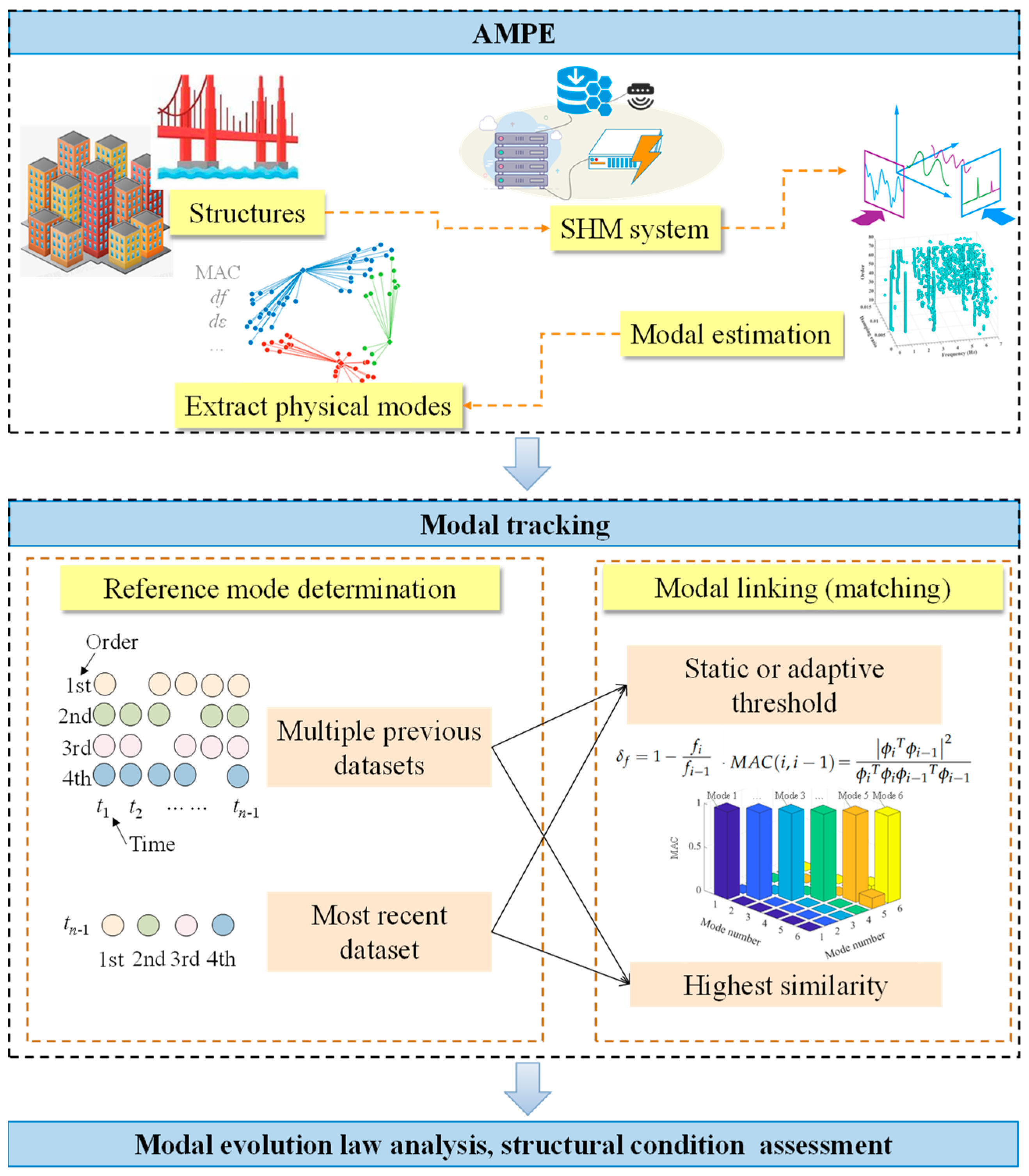
In summary, despite variations in the methodological details of modal tracking, it collectively provides crucial data support for subsequent structural assessments based on modal evolution. A standard automatic operational modal analysis process is illustrated in Figure 1.

3.2. Comparison of Two Representative Tracking Methods

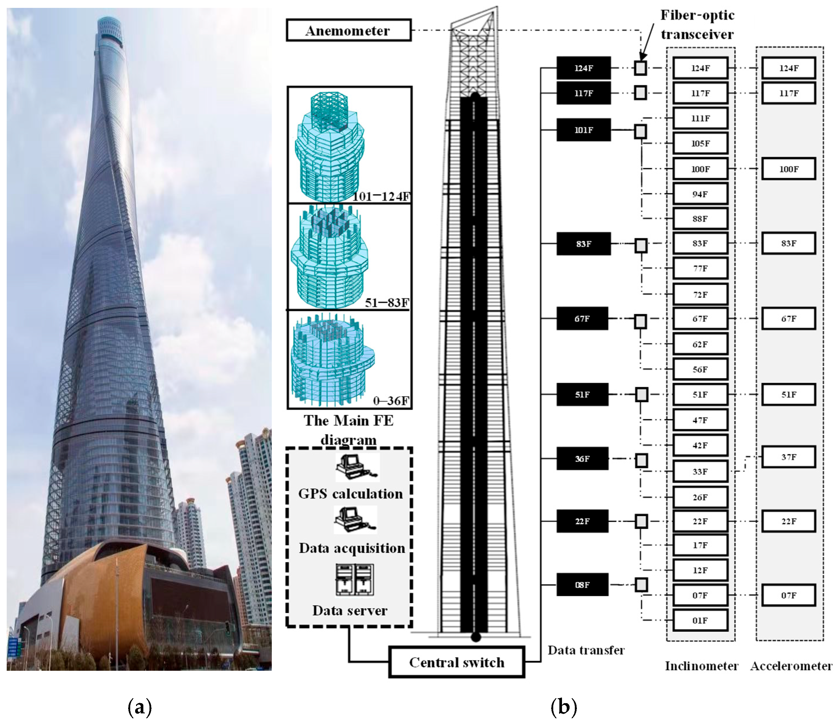
This section applies two representative methods to field measurements of a super high-rise building, providing a more intuitive comparison of their advantages and limitations. The Shanghai Tower, the tallest building in China (Figure 2a), is located in a coastal region frequently subjected to severe typhoons. As a result of the importance of this structure, a comprehensive SHM system has been deployed since its construction (Figure 2b).

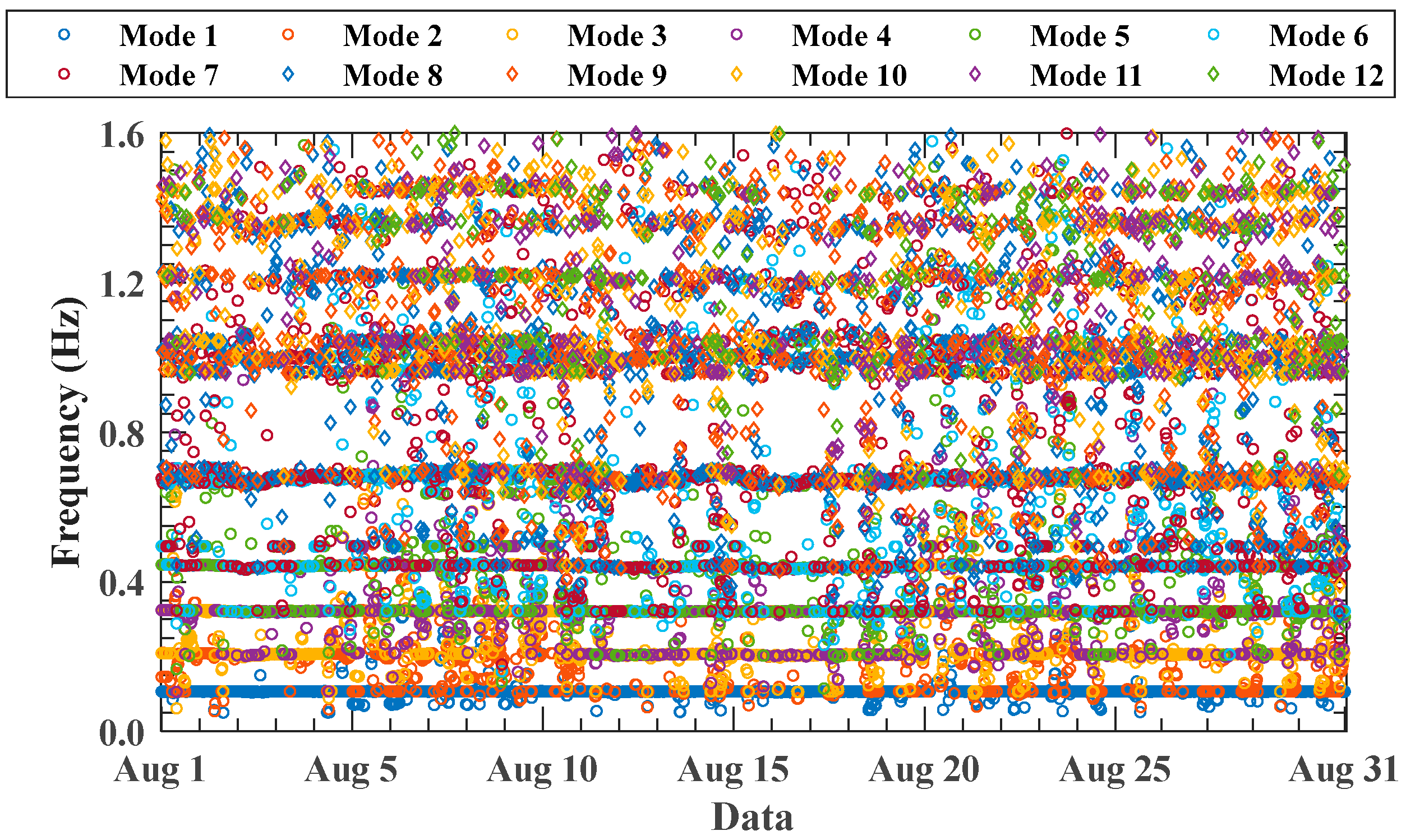
In August 2018, the tower was impacted by three typhoon events, offering unique observational conditions for modal evaluation. Based on the acceleration responses from multiple channels of the SHM system, this paper adopted the automatic SSI-COV method [16] to estimate structural frequencies, with the results shown in Figure 3. They reveal that while the AMPE method can effectively identify low-order frequencies in a brief period, it tends to generate numerous spurious modes under normal environmental excitation and may fail to detect certain physical modes. Critically, both the existence of spurious modes and the absence of physical modes perturb the determination of modal order. This suggests that AMPE may face challenges in providing long-term modal estimation, particularly for higher-order modes. Implementation of accurate and continuous modal tracking aids in monitoring long-term dynamic characteristic variations, thereby enhancing structural assessment capabilities.

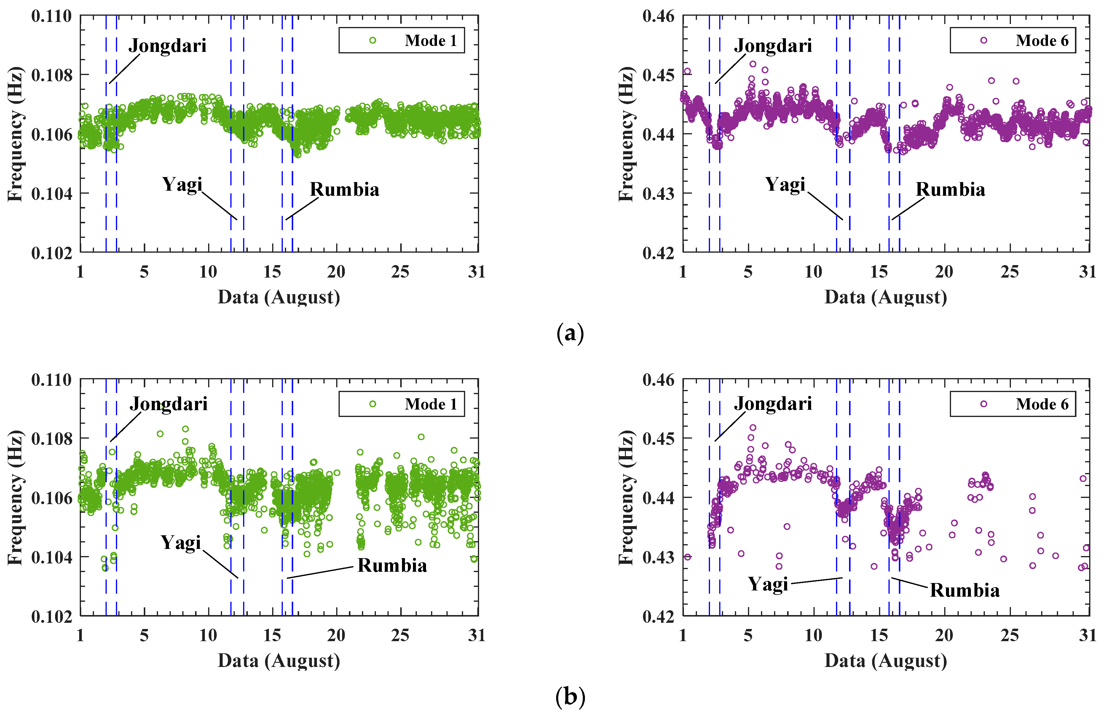
Taking Mode 1 and Mode 6 as examples, Figure 4a presents the tracking results derived from the first representative method (Method 1) [16]. In Method 1, the reference mode is determined by hierarchical clustering, and the new mode is linked only when the MAC ratio and the relative frequency difference satisfy the specified thresholds, which were set to 0.9 and 10% in this study. The analysis revealed significant variation in tracking performance among modes with different orders under uniform threshold conditions. For Mode 6, partial modes were lost during Typhoons Yagi (1814) and Rumbia (1818), despite general stability. Conversely, Mode 1 exhibited over-filtered frequency trajectories under normal wind conditions, obscuring subtle modal variations. While threshold relaxation could mitigate this issue, such an adjustment would inevitably introduce additional noisy poles and spurious modes at other orders. Consequently, unified thresholds may not be applicable for all orders of modes.

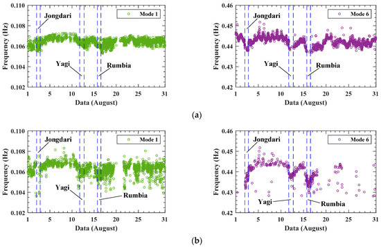
Figure 4b illustrates the modal tracking results employing Method 2 [111]. This method dynamically updates reference modes with the most recently estimated modes, while mode linking is established through a similarity matrix derived from the MMOC. A critical implementation constraint involves prespecifying the β of the modes within a targeted frequency band, and β was set to be four within 0.6 Hz in this study. Analytical results demonstrate efficacy in capturing frequency variations during typhoons. However, the mode-missing phenomenon occurs due to misclassification of the orders of reference modes during normal wind. Furthermore, this method is less robust when filtering spurious modes. In summary, distinct modal tracking methods exhibit unique advantages. Strategies capable of tracking rapidly varying modal parameters while remaining sensitive to spurious modes would facilitate the establishment of more robust methods for long-term continuous modal tracking.

4. Application of Modal Tracking

4.1. Application of Modal Tracking in Various Structures

During long-term structural operation, modal parameters inevitably experience variations induced by external factors such as wind loads, temperature fluctuations, humidity variations, and vehicular traffic (for bridges). These persistent effects lead to gradual deterioration in structural performance, thereby compromising operational safety and reliability. Consequently, employing effective modal tracking methods to precisely characterize the evolution patterns of frequencies and damping ratios throughout the structural lifecycle while elucidating the influence mechanisms of environmental factors constitutes a pivotal component of SHM [124].

Currently, modal tracking and evolution analysis have been extensively applied to various structural types: (1) long-span bridges, exemplified by the Hardanger Bridge [100], the Sutong Bridge [61], and the Infante D. Henrique Bridge [16]; (2) super high-rise buildings, including the Shanghai Tower [31], Canton Tower [125], the Shanghai World Financial Center [126], and the Ping-An International Finance Center [127]; (3) historical heritage construction, such as the Civic Tower in Rieti [105], San Pedro Apostol Church [106], Milan Cathedral [121], and Santa Maria del Carrobiolo Church [63]; (4) dams; and so on. Detailed applications and modal tracking results are systematically summarized in

Table 3. Application cases of modal tracking and corresponding results.

Reference	Application Field	Structure Name	Location	Tracked Modal Parameter	Tracking Duration	Tracking Result
Magalhães et al. [16]	Long-span arch bridge	Infante D. Henrique Bridge	Portugal	Frequency and damping ratio	2 months	Frequency fluctuated slightly
Cabboi et al. [37]	Iron arch bridge	San Michele Bridge	Italy	Frequency	About 1 month	Frequency fluctuated slightly
Fu et al. [31]	Super high-rise building	Shanghai Tower	China	Frequency	About 5.5 years	Frequency decreased
Mao et al. [61]	Long-span bridge	Sutong Bridge	China	Frequency	1 year	Frequency varied with temperature
Teng et al. [88]	Arch bridge	Rainbow Bridge	China	Frequency	320 days	Frequency fluctuated with temperature
He et al. [99]	Long-span suspension bridge	Fourth Nanjing Yangtze Bridge	China	Frequency	More than 5 weeks	Frequency varied in limited range
Dederichs et al. [100]	Suspension bridge, floating pontoon bridge	Hardanger Bridge, Bergs øysund floating pontoon bridge	Norway	Frequency	1850 datasets	Frequency fluctuated slightly
Sun et al. [104]	Concrete box-girder bridge	Z24 bridge	Switzerland	Frequency	10 months	Temporary but significant frequency increase and recovery
He et al. [111]	Footbridge	Dowling Hall footbridge	America	Frequency	2 weeks	Frequency fluctuated slightly
Yang et al. [112]	Long-span high-speed railway bridge	-	-	Frequency and damping ratio	1 year	Frequency related to train loading had greatest fluctuation
Yu and Dan [117]	Cable of a cable-stayed bridge and so on	-	-	Frequency	24 h	Frequency fluctuated with amplitude
Langone et al. [128]	Concrete box-girder bridge	Z24 bridge	Switzerland	Frequency	Several months	Damaged
Zhang et al. [129]	Long-span arch bridge	Infante D. Henrique Bridge	Portugal	Frequency and damping ratio	About 1.5 years	Frequency was higher in winter and lower during summer
Zhou and Sun [130]	Sea-crossing bridge	Donghai Bridge	China	Frequency	6 years	Frequency varied over time periods
Fu et al. [126]	Super high-rise building	Shanghai World Financial Center	China	Frequency and damping ratio	During 4 typhoons	Frequency decreased as amplitude increased
Zhou et al. [127]	Super high-rise building	Ping-An Finance Center	China	Frequency and damping ratio	2 years	Temperature had limited effects on modal parameters
Dong et al. [131]	High-rise building	Buildings A, B, C, D, E, F	Japan	Frequency and damping ratio	Long-term (years)	Decrease in frequency was related to damping ratio
Oliveira et al. [132]	Wind turbine	2.0 MW wind turbine	Portugal	Frequency and damping ratio	1 year	Frequency varied with increase in rotor speed
El-Kafafy et al. [110]	Wind turbine	Offshore wind turbine	Belgium	Frequency and damping ratio	13.67 h	Frequency fluctuated slightly
Pereira et al. [101]	Wind turbine	Wind turbine at Tocha wind farm	Portugal	Frequency and damping ratio	18 months	A strong relation between wind speed and damping
Diord et al. [109]	Sports stadium	Braga Municipal Sports Stadium	Portugal	Frequency and damping ratio	4 years	Mean frequency reduction
Pereira et al. [114]	Arch dam	Double-curvature concrete arch dam	Portugal	Frequency	3 years	Fifth mode changed significantly
Pereira et al. [103]	Arch dam	Baixo Sabor arch dam	Portugal	Frequency and damping ratio	2 years	Frequency varied with reservoir water level
Rainieri et al. [115]	Public building	Main School of Engineering building in Naples	Italy	Frequency	2 seasons	First three frequencies in summer were lower than those in winter
Gentile et al. [121]	Historical heritage construction	Milan Cathedral	Italy	Frequency	About 4 months	Frequency fluctuated with temperature
Tronci et al. [105]	Historical heritage construction	Civic Tower	Italy	Frequency and damping ratio	3 years	Frequency decreased after seismic events
Ubertini et al. [62]	Historical heritage construction	San Pietro bell tower	Italy	Frequency	9 months	Temperature produced significant changes in frequencies
Zonno et al. [108]	Historical heritage construction	Monastery of Jeronimos church	Portugal	Frequency	3230 datasets	Frequency fluctuated slightly
Zonno et al. [108]	Historical heritage construction	San Pedro Apostol Church	Peru	Frequency and damping ratio	6 months	Frequency and damping coefficient varied in range of 1–3%
Elyamani et al. [133]	Historical heritage construction	Mallorca Cathedral	Spain	Frequency	15 months	Earthquakes caused decreases in natural frequencies

. It is worth noting that certain applications in the table, despite tracking the long-term evolution patterns of modal parameters, failed to employ the standardized modal tracking methods outlined in Section 3, which may introduce spurious modes or reduce the automation of the programs.

4.2. Analysis of Modal Tracking Results

Based on modal tracking results, researchers have conducted extensive investigations into structural environmental dependencies [134,135,136,137] and damage assessment frameworks [138], with particular emphasis on establishing temperature–frequency relationship models [139,140,141]. Most studies employ correlation analysis to identify dominant influencing factors, followed by environmental effect decoupling through regression modeling [142], principal component analysis [143], or artificial neural networks [144]. The compensated modal evolution can be subsequently utilized for structural state evaluation and damage detection [145,146,147].

Empirical evidence indicates that the dynamic characteristics of bridges generally exhibit pronounced sensitivity to environmental variables (e.g., temperature and wind speed), with marked seasonal frequency fluctuations [61,148]. For instance, the Sutong Bridge manifests annual variation rates of 4.47% for its first vertical modal frequency and 8.32% for the fourth vertical mode [120]. Such environmentally driven variations may obscure frequency shifts attributable to structural damage, material deterioration, or other anomalies [149]. As summarized by Xia et al. [91], (i) under invariant boundary conditions, temperature dominates frequency fluctuations during bridge operation and (ii) bridges’ natural frequencies demonstrate a negative correlation with temperature. Notably, this empirical pattern is not universally valid. For example, the Voigt Bridge case study demonstrates positive correlations between three targeted natural frequencies and ambient temperature variations during the summer [150].

In contrast to bridge structures, wind loads, particularly typhoon effects, dominate the dynamic characteristics of super high-rise buildings with low stiffness and damping [151,152,153,154,155], whereas temperature exhibits negligible influence on their natural frequencies [127,156]. This phenomenon may be attributed to two aspects: (i) the boundary conditions of super high-rise structures resemble those of cantilever columns, facilitating the prompt release of thermal stress, and (ii) curtain wall systems separate the interior and exterior environments of a skyscraper, thereby constraining the temperature impacts on the core tube [31]. Additionally, the non-destructive nature of modern SHM techniques has promoted the application of modal tracking in historical heritage construction (generally masonry structures) [157,158]. Current implementations focus on three critical aspects: damage feature extraction [159,160], environmental effect elimination [161], and post-seismic assessment [162,163]. Particularly, the monitoring system of Milan Cathedral exemplifies advanced implementation in heritage construction due to its comprehensive sensor network [121]. Modal tracking also extends to other fields, such as dam engineering [112] and wind turbines [132].

5. Discussion and Recommendations

5.1. Automatic Modal Estimation and Modal Tracking Method

AMPE and modal tracking constitute the complete workflow of AOMA. AMPE aims to automatically extract modal parameters from individual datasets, eliminating human intervention. Research on AMPE has reached a relatively mature stage, primarily concentrating on automatic interpretation of stabilization diagrams through diverse clustering algorithms. Although these algorithms vary in their theoretical foundations, they share the same core, i.e., precise estimation of mode similarity between the poles in stabilization diagrams and rational threshold determination. Consequently, novel AMPE methods will still emerge in the future, and a pivotal challenge lies in achieving adaptive clustering thresholds to fulfill the requirements of engineering applications with diverse structures and data quality.

Due to the complexity of operational conditions, the external excitation levels of structures vary continuously over time, leading to variations in the numbers and characteristics of identifiable modes at different times. Consequently, relying solely on AMPE methods makes it challenging to ensure continuous tracking of physical modes. Modal tracking addresses this issue by establishing dynamic correspondence between current estimation results and historical references, thereby linking abundant continuous modal parameters in order on a temporal scale to obtain long-term modal evolution. The modal tracking method has remained a research hotspot in the field of SHM over the past decade or so. Nonetheless, several limitations have emerged when traditional methods are implemented in practice and require improvement:

• The determination of reference modes remains plagued by threshold sensitivity in clustering-based methods, making it challenging to achieve full automation. If modes in some orders are omitted from the reference mode list, their contributions will be disregarded in continuous modal tracking, resulting in the mode-missing phenomenon. Additionally, determining reference modes in situations with closely spaced modes presents another challenge.
• During the modal linking stage, it is necessary to define thresholds or similarity metrics to assess whether the modes estimated at different times share the same physical characteristics, which is difficult for non-experts. Specifically, small and large tolerances are suitable for tracking modes from monitoring data with high and low signal-to-noise ratios, respectively. Furthermore, changing environmental and operational conditions affect the dynamic behavior of structures, which may lead to a loss of critical information and erroneous linking, disrupting the modal tracking process.
• The criteria used to describe modal similarity must be determined carefully. Generally, the MAC, which is widely adopted in most studies, is appropriate when numerous sensors are installed at key locations on a structure but not in cases where only a few sensors are utilized.

In summary, the complexity of operational conditions makes it difficult for initial tracking methods to ensure accurate matching and effective tracking of modal parameters. To address this, it is essential not only to investigate automated strategies for determining and updating reference modes but also to propose adaptive modal matching criteria, thereby establishing fully automatic modal tracking methods for real-time online monitoring. Furthermore, reference modes determined based on multiple response sets exhibit greater robustness against spurious modes and noise but may introduce delays or even fail when tracking rapidly changing modes. In contrast, reference modes derived from the most recent response set can track sudden modal changes but are more susceptible to spurious modes. Therefore, balancing the advantages of these two tracking strategies could significantly alleviate the current limitations in modal tracking.

5.2. Modal Tracking Application

The modal evolution of infrastructure is closely related to its structural type and environmental factors, among others, necessitating empirical tracking and analysis to obtain a comprehensive understanding of this pattern. Currently, long-term modal tracking has been extended to various fields, including long-span bridges, super high-rise buildings, stadiums, dams, heritage construction, and wind turbines. Among these, modal evolution studies are more prevalent for bridges and heritage construction, primarily focusing on the coupling between natural frequencies and the ambient temperature. In contrast, modal tracking of super high-rise buildings emphasizes multi-typhoon scenarios, and studies indicate that their natural frequencies are not necessarily sensitive to temperature.

In certain cases, changes in modal parameters induced by environmental variations may obscure those caused by structural damage or degradation. Therefore, SHM based on modal tracking primarily revolves around two aspects: the elimination of environmental effects on modal parameters and service performance assessment utilizing modal variations. It is noteworthy that some studies on modal evolution have employed AMPE methods without utilizing the modal tracking frameworks discussed in Section 3.1. This suggests that AMPE methods are extensively applied in structural modal analysis, whereas standard modal tracking methods remain confined to specific scenarios. The limited adoption of modal tracking methods can be attributed to their relatively immature development, which is characterized by cumbersome procedures and insufficient automation. Consequently, there remains significant potential for advancement in both methodological development and practical applications of modal tracking in the future.

6. Conclusions

This paper commenced with a concise review of the procedural framework and inherent limitations of current automated modal estimation methods. Subsequently, it provided a comprehensive summary of methodological developments and practical applications of modal tracking. The standard modal tracking process comprises two sequential stages: reference mode determination and current mode linking. Furthermore, the determination of reference modes is systematically categorized into two primary strategies: (i) clustering based on multiple prior modes and (ii) mode estimation based on the most recent response set. Mode linking is implemented by predefined criterion thresholds or the closest similarity. The advantages and limitations of the two prevalent methods were assessed through a comparative analysis of field measurements from the Shanghai Tower. The critical conclusions and suggestions for future research are summarized below:

• The study of automatic modal estimation has been common, particularly focusing on automatic interpretation of stabilization diagrams via clustering algorithms. Future research should emphasize the development of adaptive clustering thresholds and the establishment of universal estimation frameworks adaptable to diverse structural typologies.
• The primary objective of modal tracking lies in extracting long-term modal evolution and keeping consistent modal orders. Established modal tracking methods predominantly employ clustering algorithms for reference mode determination, with mode linking typically implemented through defined criteria that integrate the MAC and relative frequency differences. This demonstrates significant research potential for automatic modal tracking in the future.
• Building upon adaptive updating for both reference modes and modal linking criteria, a pivotal challenge for modal tracking methods is balancing the capacity between the removal of spurious modes and the tracking of rapidly changing physical modes.
• While structural long-term modal evolution analysis has gained engineering interest, particularly in investigating temperature–frequency coupling models, the current immaturity of modal tracking methods constrains their popularization in various scenarios. Future research should prioritize enhanced automation in two modal tracking stages and complexity reduction in operational procedures to facilitate broader implementation across diverse structural systems.

References

- Peeters, B.; De Roeck, G. One-year monitoring of the Z24-Bridge: Environmental effects versus damage events. Earthq. Eng. Struct. Dyn. 2001, 30, 149–171. [Google Scholar] [CrossRef]
- Cheng, J.; Xiao, R.C. Probabilistic free vibration and flutter analyses of suspension bridges. Eng. Struct. 2005, 27, 1509–1518. [Google Scholar] [CrossRef]
- Shan, D.S.; Li, Q.; Khan, I.; Zhou, X.H. A novel finite element model updating method based on substructure and response surface model. Eng. Struct. 2015, 103, 147–156. [Google Scholar] [CrossRef]
- Zhang, Y.; Wang, L.Q.; Xiang, Z.H. Damage detection by mode shape squares extracted from a passing vehicle. J. Sound Vib. 2012, 331, 291–307. [Google Scholar] [CrossRef]
- Zhao, J.; Zhang, L. Structural damage identification based on the modal data change. Int. J. Eng. Manuf. 2012, 4, 59–66. [Google Scholar] [CrossRef]
- Capecchi, D.; Ciambella, J.; Pau, A.; Vestroni, F. Damage identification in a parabolic arch by means of natural frequencies, modal shapes and curvatures. Meccanica 2016, 51, 2847–2859. [Google Scholar] [CrossRef]
- Su, J.Z.; Xia, Y.; Weng, S. Review on field monitoring of high-rise structures. Struct. Control Health Monit. 2020, 27, e2629. [Google Scholar] [CrossRef]
- Shan, J.Z.; Zhang, H.Q.; Shi, W.X.; Lu, X.L. Health monitoring and field-testing of high-rise buildings: A review. Struct. Concr. 2020, 21, 1272–1285. [Google Scholar] [CrossRef]
- Bas, S.; Apaydin, N.M.; Ilki, A.; Catbas, F.N. Structural health monitoring system of the long-span bridges in Turkey. Struct. Infrastruct. Eng. 2018, 14, 425–444. [Google Scholar] [CrossRef]
- Yu, E.B.; Xu, G.J.; Han, Y.; Hu, P.; Townsend, J.F.; Li, Y.L. Bridge vibration under complex wind field and corresponding measurements: A review. J. Traffic Transp. Eng. (Engl. Ed.) 2022, 9, 339–362. [Google Scholar] [CrossRef]
- Battista, R.C.; Pfeil, M.S. Reduction of vortex-induced oscillations of Rio-Niterói bridge by dynamic control devices. J. Wind Eng. Ind. Aerodyn. 2000, 84, 273–288. [Google Scholar] [CrossRef]
- Fenerci, A.; Kvåle, K.A.; Petersen, O.W.; Ronnquist, A.; Oiseth, O. Data set from long-term wind and acceleration monitoring of the Hardanger Bridge. J. Struct. Eng. 2021, 147, 04721003. [Google Scholar] [CrossRef]
- Wu, Y.R.; Kang, F.; Wan, G.; Li, H.J. Automatic operational modal analysis for concrete arch dams integrating improved stabilization diagram with hybrid clustering algorithm. Mech. Syst. Signal Process. 2025, 224, 112011. [Google Scholar] [CrossRef]
- Masciotta, M.G.; Roque, J.C.A.; Ramos, L.F.; Lourenço, P.B. A multidisciplinary approach to assess the health state of heritage structures: The case study of the Church of Monastery of Jerónimos in Lisbon. Constr. Build. Mater. 2016, 116, 169–187. [Google Scholar] [CrossRef]
- Masciotta, M.G.; Ramos, L.F.; Lourenço, P.B. The importance of structural monitoring as a diagnosis and control tool in the restoration process of heritage structures: A case study in Portugal. J. Cult. Herit. 2017, 27, 36–47. [Google Scholar] [CrossRef]
- Magalhães, F.; Cunha, Á.; Caetano, E. Online automatic identification of the modal parameters of a long span arch bridge. Mech. Syst. Signal Process. 2009, 23, 316–329. [Google Scholar] [CrossRef]
- Reynders, E.; Houbrechts, J.; De Roeck, G. Fully automated (operational) modal analysis. Mech. Syst. Signal Process. 2012, 29, 228–250. [Google Scholar] [CrossRef]
- Chen, Z.W.; Liu, K.M.; Yan, W.J.; Zhang, J.L.; Ren, W.X. Two-stage automated operational modal analysis based on power spectrum density transmissibility and support-vector machines. Int. J. Struct. Stab. Dyn. 2021, 21, 2150068. [Google Scholar] [CrossRef]
- Rainieri, C.; Fabbrocino, G. Automated output-only dynamic identification of civil engineering structures. Mech. Syst. Signal Process. 2010, 24, 678–695. [Google Scholar] [CrossRef]
- Brincker, R.; Andersen, P.; Jacobsen, N.J.; Niels, J. Automated frequency domain decomposition for operational modal analysis. In Proceedings of the 25th International Modal Analysis Conference, Orlando, FL, USA, 19–22 February 2007. [Google Scholar]
- Vanlanduit, S.; Verboven, P.; Guillaume, P.; Schoukens, J. An automatic frequency domain modal parameter estimation algorithm. J. Sound Vib. 2003, 265, 647–661. [Google Scholar] [CrossRef]
- Peeters, B.; Van der Auweraer, H.; Vanhollebeke, F.; Guillaume, P. Operational modal analysis for estimating the dynamic properties of a stadium structure during a football game. Shock Vib. 2007, 14, 283–303. [Google Scholar] [CrossRef]
- Rainieri, C.; Fabbrocino, G. Operational Modal Analysis of Civil Engineering Structures: An Introduction and Guide for Applications; Springer: New York, NY, USA, 2014. [Google Scholar]
- Peeters, B.; Roeck, G.D. Reference-based stochastic subspace identification for output-only modal analysis. Mech. Syst. Signal Process. 1999, 13, 855–878. [Google Scholar] [CrossRef]
- Moncayo, H.; Marulanda, J.; Thomson, P. Identification and monitoring of modal parameters in aircraft structures using the natural excitation technique (NExT) combined with the eigensystem realization algorithm (ERA). J. Aerosp. Eng. 2010, 23, 99–104. [Google Scholar] [CrossRef]
- Yang, X.M.; Yi, T.H.; Qu, C.X.; Li, H.N.; Liu, H. Automated eigensystem realization algorithm for operational modal identification of bridge structures. J. Aerosp. Eng. 2019, 32, 4018148. [Google Scholar] [CrossRef]
- Van der Auweraer, H.; Peeters, B. Discriminating physical poles from mathematical poles in high order systems: Use and automation of the stabilization diagram. In Proceedings of the 21st IEEE Instrumentation and Measurement Technology Conference, Como, Italy, 18–20 May 2024. [Google Scholar]
- Carden, E.P.; Brownjohn, J.M.W. Fuzzy clustering of stability diagrams for vibration-based structural health monitoring. Comput.-Aided Civ. Infrastruct. Eng. 2008, 23, 360–372. [Google Scholar] [CrossRef]
- Ye, X.J.; Huang, P.L.; Pan, C.D.; Mei, L. Innovative stabilization diagram for automated structural modal identification based on ERA and hierarchical cluster analysis. J. Civ. Struct. Health Monit. 2021, 11, 1355–1373. [Google Scholar] [CrossRef]
- Bakir, P.G. Automation of the stabilization diagrams for subspace based system identification. Expert Syst. Appl. 2011, 38, 14390–14397. [Google Scholar] [CrossRef]
- Fu, S.H.; Wu, J.; Zhang, Q.L.; Xie, B. Automated identification and long-term tracking of modal parameters for a super high-rise building. J. Build. Eng. 2024, 95, 110141. [Google Scholar] [CrossRef]
- Mellinger, P.; Döhler, M.; Mevel, L. Variance estimation of modal parameters from output-only and input/output subspace-based system identification. J. Sound Vib. 2016, 379, 1–27. [Google Scholar] [CrossRef]
- Tondreau, G.; Deraemaeker, A. Numerical and experimental analysis of uncertainty on modal parameters estimated with the stochastic subspace method. J. Sound Vib. 2014, 333, 4376–4401. [Google Scholar] [CrossRef]
- Cunha, Á.; Caetano, E.; Magalhães, F.; Moutinho, C. Recent perspectives in dynamic testing and monitoring of bridges. Struct. Control Health Monit. 2013, 20, 853–877. [Google Scholar] [CrossRef]
- Kita, A.; Cavalagli, N.; Ubertini, F. Temperature effects on static and dynamic behavior of Consoli Palace in Gubbio, Italy. Mech. Syst. Signal Process. 2019, 120, 180–202. [Google Scholar] [CrossRef]
- Huang, T.L.; Chen, H.P. Mode identifiability of a cable-stayed bridge using modal contribution index. Smart Struct. Syst. 2017, 20, 115–126. [Google Scholar] [CrossRef]
- Cabboi, A.; Magalhães, F.; Gentile, C.; Cunha, Á. Automated modal identification and tracking: Application to an iron arch bridge. Struct. Control Health Monit. 2017, 24, e1854. [Google Scholar] [CrossRef]
- Magalhães, F.; Cunha, A.; Caetano, E. Vibration based structural health monitoring of an arch bridge: From automated OMA to damage detection. Mech. Syst. Signal Process. 2012, 28, 212–228. [Google Scholar] [CrossRef]
- Giordano, P.F.; Ubertini, F.; Cavalagli, N.; Kita, A.; Masciotta, M.G. Four years of structural health monitoring of the San Pietro bell tower in Perugia, Italy: Two years before the earthquake versus two years after. Int. J. Mason. Res. Innov. 2020, 5, 445–467. [Google Scholar] [CrossRef]
- Oliveira, G.; Magalhães, F.; Cunha, Á.; Caetano, E. Vibration-based damage detection in a wind turbine using 1 year of data. Struct. Control Health Monit. 2018, 25, e2238. [Google Scholar] [CrossRef]
- Busatta, F.; Gentile, C.; Saisi, A. Structural health monitoring of a centenary iron arch bridge. In Proceedings of the 3rd International Symposium on Life-Cycle Civil Engineering, Vienna, Austria, 3–6 October 2012. [Google Scholar]
- Bao, Y.Q.; Chen, Z.C.; Wei, S.Y.; Xu, Y.; Tang, Z.Y.; Li, H. The state of the art of data science and engineering in structural health monitoring. Engineering 2019, 5, 234–242. [Google Scholar] [CrossRef]
- Yang, X.M.; Yi, T.H.; Qu, C.X.; Li, H.N.; Liu, H. Continuous tracking of bridge modal parameters based on subspace correlations. Struct. Control Health Monit. 2020, 27, e2615. [Google Scholar] [CrossRef]
- Nicoletti, V.; Quarchioni, S.; Amico, L.; Gara, F. Assessment of different optimal sensor placement methods for dynamic monitoring of civil structures and infrastructures. Struct. Infrastruct. Eng. 2024, 1–16. [Google Scholar] [CrossRef]
- Chai, W.H.; Yang, Y.X.; Yu, H.B. Optimal sensor placement of bridge structure based on sensitivity-effective independence method. IET Circuits Devices Syst. 2022, 16, 125–135. [Google Scholar] [CrossRef]
- Shi, Q.H.; Wang, X.J.; Chen, W.P.; Hu, K.J. Optimal sensor placement method considering the importance of structural performance degradation for the allowable loadings for damage identification. Appl. Math. Model. 2020, 86, 384–403. [Google Scholar] [CrossRef]
- Silva, M.; Santos, A.; Figueiredo, E.; Santos, R.; Sales, C.; Costa, J.C.W.A. A novel unsupervised approach based on a genetic algorithm for structural damage detection in bridges. Eng. Appl. Artif. Intell. 2018, 58, 2099–2118. [Google Scholar] [CrossRef]
- Moazenzadeh, R.; Mohammadi, B.; Shamshirband, S.; Chau, K.W. Coupling a firefly algorithm with support vector regression to predict evaporation in northern Iran. Eng. Appl. Comput. Fluid Mech. 2018, 12, 584–597. [Google Scholar] [CrossRef]
- Ou, J.P.; Li, H. Structural health monitoring in mainland China: Review and future trends. Struct. Health Monit.-Int. J. 2010, 9, 219–231. [Google Scholar] [CrossRef]
- Soyoz, S.; Feng, M.Q. Long-term monitoring and identification of bridge structural parameters. Comput.-Aided Civ. Infrastruct. Eng. 2009, 24, 82–92. [Google Scholar] [CrossRef]
- Zonno, G.; Aguilar, R.; Boroschek, R.; Lourenço, P.B. Environmental and ambient vibration monitoring of historical adobe buildings: Applications in emblematic Andean churches. Int. J. Archit. Herit. 2019, 15, 1113–1129. [Google Scholar] [CrossRef]
- Ramos, L.F.; Marques, L.; Lourenço, P.B.; De Roeck, G.; Campos-Costa, A.; Roque, J. Monitoring historical masonry structures with operational modal analysis: Two case studies. Mech. Syst. Signal Process. 2010, 24, 1291–1305. [Google Scholar] [CrossRef]
- Xiong, H.B.; Cao, J.X.; Zhang, F.L.; Ou, X.; Chen, C.J. Investigation of the SHM-oriented model and dynamic characteristics of a super-tall building. Smart Struct. Syst. 2019, 23, 295–306. [Google Scholar] [CrossRef]
- Su, J.Z.; Xia, Y.; Chen, L.; Zhao, X.; Zhang, Q.L.; Xu, Y.L.; Ding, J.M.; Xiong, H.B.; Ma, R.J.; Lv, X.L.; et al. Long-term structural performance monitoring system for the Shanghai Tower. J. Civ. Struct. Health Monit. 2013, 3, 49–61. [Google Scholar] [CrossRef]
- Devriendt, C.; Magalhães, F.; Weijtjens, W.; De Sitter, G.; Cunha, Á.; Guillaume, P. Structural health monitoring of offshore wind turbines using automated operational modal analysis. Struct. Health Monit.-Int. J. 2014, 13, 644–659. [Google Scholar] [CrossRef]
- Oliveira, G.; Magalhães, F.; Cunha, Á.; Caetano, E. Development and implementation of a continuous dynamic monitoring system in a wind turbine. J. Civ. Struct. Health 2016, 6, 343–353. [Google Scholar] [CrossRef]
- Hu, W.H.; Tang, D.H.; Wang, M.; Liu, J.L.; Li, Z.H.; Lu, W.; Teng, J.; Said, S.; Rohrmann, R.G. Resonance monitoring of a horizontal wind turbine by strain-based automated operational modal analysis. Energies 2020, 13, 579. [Google Scholar] [CrossRef]
- Martins, N.; Caetano, E.; Diord, S.; Magalhães, F.; Cunha, Á. Dynamic monitoring of a stadium suspension roof: Wind and temperature influence on modal parameters and structural response. Eng. Struct. 2014, 59, 80–94. [Google Scholar] [CrossRef]
- Darbre, G.R.; Proulx, J. Continuous ambient-vibration monitoring of the arch dam of Mauvoisin. Earthq. Eng. Struct. Dyn. 2002, 31, 475–480. [Google Scholar] [CrossRef]
- Pereira, S.; Magalhães, F.; Gomes, J.P.; Cunha, Á.; Lemos, J.V. Dynamic monitoring of a concrete arch dam during the first filling of the reservoir. Eng. Struct. 2018, 174, 548–560. [Google Scholar] [CrossRef]
- Mao, J.X.; Wang, H.; Spencer, B.F. Gaussian mixture model for automated tracking of modal parameters of long-span bridge. Smart Struct. Syst. 2019, 24, 243–256. [Google Scholar] [CrossRef]
- Ubertini, F.; Comanducci, G.; Cavalagli, N.; Pisello, A.L.; Materazzi, A.L.; Cotana, F. Environmental effects on natural frequencies of the San Pietro bell tower in Perugia, Italy, and their removal for structural performance assessment. Mech. Syst. Signal Process. 2017, 82, 307–322. [Google Scholar] [CrossRef]
- Saisi, A.; Gentile, C.; Ruccolo, A. Continuous monitoring of a challenging heritage tower in Monza, Italy. J. Civ. Struct. Health Monit. 2018, 8, 77–90. [Google Scholar] [CrossRef]
- Van der Auweraer, H.; Guillaume, P.; Verboven, P.; Vanlanduit, S. Application of a fast-stabilizing frequency domain parameter estimation method. J. Dyn. Syst. Meas. Control 2001, 123, 651658. [Google Scholar] [CrossRef]
- Faurre, P.L. Stochastic realization algorithms. Math. Sci. Eng. 1976, 126, 1–25. [Google Scholar] [CrossRef]
- Juang, J.N.; Pappa, R.S. An eigensystem realization algorithm for modal parameter identification and model reduction. J. Guid. 1985, 8, 620–627. [Google Scholar] [CrossRef]
- Tronci, E.M.; De Angelis, M.; Betti, R.; Altomare, V. Multi-stage semi-automated methodology for modal parameters estimation adopting parametric system identification algorithms. Mech. Syst. Signal Process. 2022, 165, 108317. [Google Scholar] [CrossRef]
- Wu, W.H.; Wang, S.W.; Chen, C.C.; Lai, G. Application of stochastic subspace identification for stay cables with an alternative stabilization diagram and hierarchical sifting process. Struct. Control Health Monit. 2016, 23, 1194–1213. [Google Scholar] [CrossRef]
- Fan, G.; Li, J.; Hao, H. Improved automated operational modal identification of structures based on clustering. Struct. Control Health Monit. 2019, 26, e2450. [Google Scholar] [CrossRef]
- Ubertini, F.; Gentile, C.; Materazzi, A.L. Automated modal identification in operational conditions and its application to bridges. Eng. Struct. 2013, 46, 264–278. [Google Scholar] [CrossRef]
- Scionti, M.; Lanslots, J.P. Stabilisation diagrams: Pole identification using fuzzy clustering techniques. Adv. Eng. Softw. 2005, 36, 768–779. [Google Scholar] [CrossRef]
- He, M.; Liang, P.; Liu, J.X.; Liang, Z.Q. Review and comparison of methods and benchmarks for automatic modal identification based on stabilization diagram. J. Traffic Transp. Eng. (Engl. Ed.) 2024, 11, 209–224. [Google Scholar] [CrossRef]
- Neu, E.; Janser, F.; Khatibi, A.A.; Orifici, A.C. Fully automated operational modal analysis using multi-stage clustering. Mech. Syst. Signal Process. 2017, 84, 308–323. [Google Scholar] [CrossRef]
- Charbonnel, P.É. Fuzzy-driven strategy for fully automated modal analysis: Application to the SMART2013 shaking-table test campaign. Mech. Syst. Signal Process. 2021, 152, 107388. [Google Scholar] [CrossRef]
- Pappa, R.S.; Elliott, K.B.; Schenk, A. Consistent-mode indicator for the eigensystem realization algorithm. J. Guid. Control Dyn. 1993, 16, 852–858. [Google Scholar] [CrossRef]
- Heylen, W.; Lammens, S.; Sas, P. Modal Analysis Theory and Testing; Katholieke Universteit Leuven, Departement Werktuigkunde: Leuven, Belgium, 1997; Available online: https://lirias.kuleuven.be/handle/123456789/155116 (accessed on 20 November 2024).
- Allemang, R.J.; Brown, D.L. A correlation coefficient for modal vector analysis. In Proceedings of the 1st International Modal Analysis Conference, Orlando, FL, USA, 8–10 November 1982; pp. 110–116. [Google Scholar]
- Lardies, J.; Ta, M.N. Modal parameter identification of stay cables from output-only measurements. Mech. Syst. Signal Process. 2011, 25, 133–150. [Google Scholar] [CrossRef]
- Reynders, E.; De Roeck, G. Reference-based combined deterministic-stochastic subspace identification for experimental and operational modal analysis. Mech. Syst. Signal Process. 2008, 22, 617–637. [Google Scholar] [CrossRef]
- Pecorelli, M.L.; Ceravolo, R.; Epicoco, R. An automatic modal identification procedure for the permanent dynamic monitoring of the Sanctuary of Vicoforte. Int. J. Archit. Herit. 2020, 14, 630–644. [Google Scholar] [CrossRef]
- Mao, J.X.; Wang, H.; Fu, Y.G.; Spencer, B.F. Automated modal identification using principal component and cluster analysis: Application to a long-span cable-stayed bridge. Struct. Control Health Monit. 2019, 26, e2430. [Google Scholar] [CrossRef]
- Zini, G.; Betti, M.; Bartoli, G. A quality-based automated procedure for operational modal analysis. Mech. Syst. Signal Process. 2022, 164, 108173. [Google Scholar] [CrossRef]
- He, M.; Liang, P.; Li, J.; Zhang, Y.; Liu, Y.J. Fully automated precise operational modal identification. Eng. Struct. 2021, 234, 111988. [Google Scholar] [CrossRef]
- Qin, X.R.; Liu, J.H.; Yu, C.Q.; Wang, Y.L.; Zhang, Q.; Sun, Y.T. Automatic identification of modal parameters based on interval perturbation and double-layer fuzzy clustering. J. Vib. Shock 2020, 39, 122–127. [Google Scholar]
- Sun, M.; Makki Alamdari, M.; Kalhori, H. Automated operational modal analysis of a cable-stayed bridge. J. Bridge Eng. 2017, 22, 05017012. [Google Scholar] [CrossRef]
- Boroschek, R.L.; Bilbao, J.A. Interpretation of stabilization diagrams using density-based clustering algorithm. Eng. Struct. 2019, 178, 245–257. [Google Scholar] [CrossRef]
- Li, S.; Pan, J.W.; Luo, G.H.; Wang, J.T. Automatic modal parameter identification of high arch dams: Feasibility verification. Earthq. Eng. Eng. Vib. 2020, 19, 953–965. [Google Scholar] [CrossRef]
- Teng, J.; Tang, D.H.; Zhang, X.; Hu, W.H.; Said, S.; Rohrmann, R.G. Automated modal analysis for tracking structural change during construction and operation phases. Sensors 2019, 19, 927. [Google Scholar] [CrossRef] [PubMed]
- Zhang, X.L.; Zhou, W.S.; Huang, Y.; Li, H. Automatic identification of structural modal parameters based on density peaks clustering algorithm. Struct. Control Health Monit. 2022, 29, e3138. [Google Scholar] [CrossRef]
- Pan, H.R.; Li, Y.; Deng, T.; Fu, J.Y. An improved stochastic subspace identification approach for automated operational modal analysis of high-rise buildings. J. Build. Eng. 2024, 89, 109267. [Google Scholar] [CrossRef]
- Xia, Y.; Chen, B.; Weng, S.; Ni, Y.Q.; Xu, Y.L. Temperature effect on vibration properties of civil structures: A literature review and case studies. J. Civ. Struct. Health Monit. 2012, 2, 29–46. [Google Scholar] [CrossRef]
- Wu, J.; Xu, H.J.; Zhang, Q.L. Dynamic performance evaluation of Shanghai Tower under winds based on full-scale data. Struct. Des. Tall Spec. Build. 2019, 28, e1611. [Google Scholar] [CrossRef]
- Yang, B.; Pan, L.C.; Zhu, H.T.; Sun, S.Y.; Zhang, Q.L. Spatiotemporal correlation analysis of the dynamic response of supertall buildings under ambient wind conditions. Struct. Des. Tall Spec. Build. 2022, 31, e1914. [Google Scholar] [CrossRef]
- Wu, J.; Hu, N.T.; Dong, Y.; Zhang, Q.L. Monitoring dynamic characteristics of 600 m+ Shanghai Tower during two consecutive typhoons. Struct. Control Health Monit. 2021, 28, e2666. [Google Scholar] [CrossRef]
- He, Y.C.; Li, Q.S. Dynamic responses of a 492-m-high tall building with active tuned mass damping system during a typhoon. Struct. Control Health Monit. 2013, 21, 705–720. [Google Scholar] [CrossRef]
- Zhang, Q.L.; Luo, X.Q.; Ding, J.M.; Xie, B.; Gao, X.Z. Dynamic response evaluation on TMD and main tower of Shanghai Tower subjected to Typhoon In-Fa. Struct. Des. Tall Spec. Build. 2022, 31, e1929. [Google Scholar] [CrossRef]
- Zhou, K.; Li, Q.S. Vibration mitigation performance of active tuned mass damper in a super high-rise building during multiple tropical storms. Eng. Struct. 2022, 269, 114840. [Google Scholar] [CrossRef]
- Au, S.K.; Brownjohn, J.M.W.; Li, B.B.; Raby, A. Understanding and managing identification uncertainty of close modes in operational modal analysis. Mech. Syst. Signal Process. 2021, 147, 107018. [Google Scholar] [CrossRef]
- He, M.; Liang, P.; Obrien, E.; Sun, X.; Zhang, Y. Continuous modal identification and tracking of a long-span suspension bridge using a robust mixed-clustering method. J. Bridge Eng. 2022, 27, 05022001. [Google Scholar] [CrossRef]
- Dederichs, A.C.; Øiseth, O. A novel and near-automatic mode tracking algorithm for civil infrastructure. J. Sound Vib. 2024, 573, 118217. [Google Scholar] [CrossRef]
- Pereira, S.; Pacheco, J.; Pimenta, F.; Moutinho, C.; Cunha, Á.; Magalhães, F. Contributions for enhanced tracking of (onshore) wind turbines modal parameters. Eng. Struct. 2023, 274, 115120. [Google Scholar] [CrossRef]
- Peeters, B.; Van der Auweraer, H.; Guillaume, P.; Leuridan, J. The PolyMAX frequency domain method: A new standard for modal parameter estimation. Shock Vib. 2004, 11, 523692. [Google Scholar] [CrossRef]
- Pereira, S.; Reynders, E.; Magalhães, F.; Cunha, Á.; Gomes, J.P. The role of modal parameters uncertainty estimation in automated modal identification, modal tracking and data normalization. Eng. Struct. 2020, 224, 111208. [Google Scholar] [CrossRef]
- Sun, S.Y.; Yang, B.; Zhang, Q.L.; Wüchner, R.; Pan, L.C.; Zhu, H.T. Long-term continuous automatic modal tracking algorithm based on Bayesian inference. Struct. Health Monit.-Int. J. 2023, 23, 1530–1546. [Google Scholar] [CrossRef]
- Tronci, E.M.; De Angelis, M.; Betti, R.; Altomare, V. Vibration-based structural health monitoring of a RC-masonry tower equipped with non-conventional TMD. Eng. Struct. 2020, 224, 111212. [Google Scholar] [CrossRef]
- Tronci, E.M.; De Angelis, M.; Betti, R.; Altomare, V. Semi-automated operational modal analysis methodology to optimize modal parameter estimation. J. Optim. Theory Appl. 2020, 187, 842–854. [Google Scholar] [CrossRef]
- Ubertini, F.; Comanducci, G.; Cavalagli, N. Vibration-based structural health monitoring of a historic bell-tower using output-only measurements and multivariate statistical analysis. Struct. Health Monit.-Int. J. 2016, 15, 438–457. [Google Scholar] [CrossRef]
- Zonno, G.; Aguilar, R.; Boroschek, R.; Lourenço, P.B. Automated long-term dynamic monitoring using hierarchical clustering and adaptive modal tracking: Validation and applications. J. Civ. Struct. Health Monit. 2018, 8, 791–808. [Google Scholar] [CrossRef]
- Diord, S.; Magalhães, F.; Cunha, Á.; Caetano, E.; Martins, N. Automated modal tracking in a football stadium suspension roof for detection of structural changes. Struct. Control Health Monit. 2017, 24, e2006. [Google Scholar] [CrossRef]
- El-Kafafy, M.; Gioia, N.; Guillaume, P.; Helsen, J. Long-term automatic tracking of the modal parameters of an offshore wind turbine drivetrain system in standstill condition. In Rotating Machinery, Vibro-Acoustics & Laser Vibrometry; Springer International Publishing: Cham, Switzerland, 2019; Volume 7, pp. 91–99. [Google Scholar] [CrossRef]
- He, M.; Liang, P.; Zhang, Y.; Yang, F.; Liu, J.X. Unified method for fully automated modal identification and tracking with consideration of sensor deployment. Eng. Struct. 2022, 260, 114223. [Google Scholar] [CrossRef]
- Yang, X.M.; Li, H.N.; Yi, T.H.; Qu, C.X.; Liu, H. Fully automated modal tracking for long-span high-speed railway bridges. Adv. Struct. Eng. 2022, 25, 3475–3491. [Google Scholar] [CrossRef]
- Yazdani-Shavakand, M.; Ahmadi-Shokouh, J.; Dashti, H. A fast multi-structural tracking method for characteristic modes with the ability to identify and amend errors. IET Microw. Antennas Propag. 2023, 17, 62–74. [Google Scholar] [CrossRef]
- Pereira, S.; Magalhães, F.; Gomes, J.P.; Cunha, Á. Modal tracking under large environmental influence. J. Civ. Struct. Health Monit. 2022, 12, 179–190. [Google Scholar] [CrossRef]
- Rainieri, C.; Fabbrocino, G.; Cosenza, E. Near real-time tracking of dynamic properties for standalone structural health monitoring systems. Mech. Syst. Signal Process. 2011, 25, 3010–3026. [Google Scholar] [CrossRef]
- Magalhães, F.; Cunha, Á.; Caetano, E. Dynamic monitoring of a long span arch bridge. Eng. Struct. 2008, 30, 3034–3044. [Google Scholar] [CrossRef]
- Yu, X.W.; Dan, D.H. Online frequency and amplitude tracking in structural vibrations under environment using APES spectrum postprocessing and Kalman filtering. Eng. Struct. 2022, 259, 114175. [Google Scholar] [CrossRef]
- Li, J.; Stoica, P. An adaptive filtering approach to spectral estimation and SAR imaging. IEEE Trans. Signal Process. 1996, 44, 1469–1484. [Google Scholar] [CrossRef]
- Zhong, K.; Chang, C.C. Tracking dynamic characteristics of structures using output-only recursive combined subspace identification technique. J. Eng. Mech. 2020, 146, 04020035. [Google Scholar] [CrossRef]
- Mao, J.X.; Wang, H.; Feng, D.M.; Tao, T.Y.; Zheng, W.Z. Investigation of dynamic properties of long-span cable-stayed bridges based on one-year monitoring data under normal operating condition. Struct. Control Health Monit. 2018, 25, e2146. [Google Scholar] [CrossRef]
- Gentile, C.; Ruccolo, A.; Canali, F. Continuous monitoring of the Milan Cathedral: Dynamic characteristics and vibration-based SHM. J. Civ. Struct. Health Monit. 2019, 9, 671–688. [Google Scholar] [CrossRef]
- Fu, S.H.; Wu, J.; Zhang, Q.L.; Xie, B. Robust and efficient synchronization for structural health monitoring data with arbitrary time lags. Eng. Struct. 2025, 322, 119183. [Google Scholar] [CrossRef]
- Yang, M.X.; Wu, J.; Zhang, Q.L. Inclination and acceleration data fusion for two-dimensional dynamic displacements and mode shapes identification of super high-rise buildings considering time delay. Mech. Syst. Signal Process. 2025, 223, 111938. [Google Scholar] [CrossRef]
- Yu, L.; Yin, T. Damage identification in frame structures based on FE model updating. J. Vib. Acoust. 2010, 132, 051007. [Google Scholar] [CrossRef]
- Ye, X.J.; Chen, B.C. Model updating and variability analysis of modal parameters for super high-rise structure. Concurr. Comput. Pract. Exp. 2019, 31, e4712. [Google Scholar] [CrossRef]
- Fu, G.Q.; Quan, Y.; Gu, M.; Huang, Z.F.; Feng, C.D. Dynamic performance evaluation of a 492 m super high-rise building with active tuned mass dampers during four consecutive landfall typhoons within a month. J. Build. Eng. 2022, 61, 105259. [Google Scholar] [CrossRef]
- Zhou, K.; Li, Q.S.; Zhi, L.H.; Han, X.L.; Xu, K. Investigation of modal parameters of a 600-m-tall skyscraper based on two-year-long structural health monitoring data and five typhoons measurements. Eng. Struct. 2023, 274, 115162. [Google Scholar] [CrossRef]
- Langone, R.; Reynders, E.; Mehrkanoon, S.; Suykens, J.A.K. Automated structural health monitoring based on adaptive kernel spectral clustering. Mech. Syst. Signal Process. 2017, 90, 64–78. [Google Scholar] [CrossRef]
- Zhang, G.; Moutinho, C.; Magalhães, F. Continuous dynamic monitoring of a large-span arch bridge with wireless nodes based on MEMS accelerometers. Struct. Control Health Monit. 2022, 29, e2963. [Google Scholar] [CrossRef]
- Zhou, Y.; Sun, L.M. Effects of environmental and operational actions on the modal frequency variations of a sea-crossing bridge: A periodicity perspective. Mech. Syst. Signal Process. 2019, 131, 505–523. [Google Scholar] [CrossRef]
- Dong, Y.F.; Tian, H.; Zhang, M.; Wei, L.J. Long-term monitoring of dynamic characteristics of high-rise and super high-rise buildings using strong motion records. Adv. Mech. Eng. 2021, 13, 168781402110672. [Google Scholar] [CrossRef]
- Oliveira, G.; Magalhães, F.; Cunha, Á.; Caetano, E. Automated modal tracking and fatigue assessment of a wind turbine based on continuous dynamic monitoring. MATEC Web Conf. 2015, 24, 04005. [Google Scholar] [CrossRef]
- Elyamani, A.; Caselles, O.; Roca, P.; Clapes, J. Dynamic investigation of a large historical cathedral. Struct. Control Health Monit. 2017, 24, e1885. [Google Scholar] [CrossRef]
- Xia, Y.; Hao, H.; Zanardo, G.; Deeks, A. Long term vibration monitoring of an RC slab: Temperature and humidity effect. Eng. Struct. 2006, 28, 441–452. [Google Scholar] [CrossRef]
- Li, H.; Li, S.L.; Ou, J.P.; Li, H.W. Modal identification of bridges under varying environmental conditions: Temperature and wind effects. Struct. Control Health Monit. 2010, 17, 495–512. [Google Scholar] [CrossRef]
- Reynders, E.; Wursten, G.; De Roeck, G. Output-only structural health monitoring in changing environmental conditions by means of nonlinear system identification. Struct. Health Monit.-Int. J. 2014, 13, 82–93. [Google Scholar] [CrossRef]
- Behmanesh, I.; Moaveni, B. Accounting for environmental variability, modeling errors, and parameter estimation uncertainties in structural identification. J. Sound Vib. 2016, 374, 92–110. [Google Scholar] [CrossRef]
- Wah, W.S.L.; Chen, Y.T.; Roberts, G.W.; Elamin, A. Separating damage from environmental effects affecting civil structures for near real-time damage detection. Struct. Health Monit.-Int. J. 2018, 17, 850–868. [Google Scholar] [CrossRef]
- Adams, R.D.; Cawley, P.; Pye, C.J.; Stone, B.J. A vibration technique for non-destructively assessing the integrity of structures. J. Mech. Eng. Sci. 1978, 20, 93–100. [Google Scholar] [CrossRef]
- Ni, Y.Q.; Hua, X.G.; Fan, K.Q.; Ko, J.M. Correlating modal properties with temperature using long-term monitoring data and support vector machine technique. Eng. Struct. 2005, 27, 1762–1773. [Google Scholar] [CrossRef]
- Hu, W.H.; Cunha, Á.; Caetano, E.; Rohrmann, R.G.; Said, S.; Teng, J. Comparison of different statistical approaches for removing environmental/operational effects for massive data continuously collected from footbridges. Struct. Control Health Monit. 2017, 24, e1955. [Google Scholar] [CrossRef]
- Moser, P.; Moaveni, B. Environmental effects on the identified natural frequencies of the Dowling Hall Footbridge. Mech. Syst. Signal Process. 2011, 25, 2336–2357. [Google Scholar] [CrossRef]
- Hu, W.H.; Moutinho, C.; Caetano, E.; Magalhães, F.; Cunha, Á. Continuous dynamic monitoring of a lively footbridge for serviceability assessment and damage detection. Mech. Syst. Signal Process. 2012, 33, 38–55. [Google Scholar] [CrossRef]
- Zhou, X.T.; Ni, Y.Q.; Zhang, F.L. Damage localization of cable-supported bridges using modal frequency data and probabilistic neural network. Math. Probl. Eng. 2014, 2014, 837963. [Google Scholar] [CrossRef]
- Deraemaeker, A.; Worden, K. A comparison of linear approaches to filter out environmental effects in structural health monitoring. Mech. Syst. Signal Process. 2018, 105, 1–15. [Google Scholar] [CrossRef]
- Ding, Z.H.; Li, J.; Hao, H. Structural damage identification using improved Jaya algorithm based on sparse regularization and Bayesian inference. Mech. Syst. Signal Process. 2019, 132, 211–231. [Google Scholar] [CrossRef]
- Sarmadi, H.; Entezami, A.; Salar, M.; De Michele, C. Bridge health monitoring in environmental variability by new clustering and threshold estimation methods. J. Civ. Struct. Health Monit. 2021, 11, 629–644. [Google Scholar] [CrossRef]
- Hu, W.H.; Caetano, E.; Cunha, Á. Structural health monitoring of a stress-ribbon footbridge. Eng. Struct. 2013, 57, 578–593. [Google Scholar] [CrossRef]
- Sohn, H. Effects of environmental and operational variability on structural health monitoring. Philos. Trans. R. Soc. A-Math. Phys. Eng. Sci. 2007, 365, 539–560. [Google Scholar] [CrossRef] [PubMed]
- He, X.F. Vibration-Based Damage Identification and Health Monitoring of Civil Structures. Ph.D. Thesis, University of California, San Diego, CA, USA, 2008. Available online: https://escholarship.org/uc/item/9dk7q06h (accessed on 28 October 2024).
- Li, X.; Li, Q.S. Monitoring structural performance of a supertall building during 14 tropical cyclones. J. Struct. Eng. 2018, 144, 04018176. [Google Scholar] [CrossRef]
- Yi, J.; Zhang, J.W.; Li, Q.S. Dynamic characteristics and wind-induced responses of a super-tall building during typhoons. J. Wind Eng. Ind. Aerodyn. 2013, 121, 116–130. [Google Scholar] [CrossRef]
- Kijewski-Correa, T.; Pirnia, J.D. Dynamic behavior of tall buildings under wind: Insights from full-scale monitoring. Struct. Des. Tall Spec. Build. 2007, 16, 471–486. [Google Scholar] [CrossRef]
- Fu, J.Y.; Wu, J.R.; Xu, A.; Li, Q.S.; Xiao, Y.Q. Full-scale measurements of wind effects on Guangzhou West Tower. Eng. Struct. 2012, 35, 120–139. [Google Scholar] [CrossRef]
- Yang, M.X.; Wu, J.; Zhang, Q.L. GNSS and accelerometer data fusion by variational Bayesian adaptive multi-rate Kalman filtering for dynamic displacement estimation of super high-rise buildings. Eng. Struct. 2025, 325, 119396. [Google Scholar] [CrossRef]
- Sun, M.M.; Li, Q.S.; Han, X.L. Investigation of long-term modal properties of a supertall building under environmental and operational variations. J. Build. Eng. 2022, 62, 105439. [Google Scholar] [CrossRef]
- Cabboi, A.; Gentile, C.; Saisi, A. Frequency tracking and FE model identification of a masonry tower. In Proceedings of the 5th International Operational Modal Analysis Conferences, Guimarães, Portugal, 13–15 May 2013. [Google Scholar]
- Saisi, A.; Gentile, C.; Guidobaldi, M. Post-earthquake continuous dynamic monitoring of the Gabbia Tower in Mantua, Italy. Constr. Build. Mater. 2015, 81, 101–112. [Google Scholar] [CrossRef]
- Gentile, C.; Guidobaldi, M.; Saisi, A. One-year dynamic monitoring of a historic tower: Damage detection under changing environment. Meccanica 2016, 51, 2873–2889. [Google Scholar] [CrossRef]
- Cabboi, A.; Gentile, C.; Saisi, A. From continuous vibration monitoring to FEM-based damage assessment: Application on a stone-masonry tower. Constr. Build. Mater. 2017, 156, 252–265. [Google Scholar] [CrossRef]
- Azzara, R.M.; De Roeck, G.; Girardi, M.; Padovani, C.; Pellegrini, D.; Reynders, E. The influence of environmental parameters on the dynamic behaviour of the San Frediano bell tower in Lucca. Eng. Struct. 2018, 156, 175–187. [Google Scholar] [CrossRef]
- Ubertini, F.; Cavalagli, N.; Kita, A.; Comanducci, G. Assessment of a monumental masonry bell-tower after 2016 Central Italy seismic sequence by long-term SHM. Bull. Earthq. Eng. 2018, 16, 775–801. [Google Scholar] [CrossRef]
- Lorenzoni, F.; Caldon, M.; da Porto, F.; Modena, C.; Aokiet, T. Post-earthquake controls and damage detection through structural health monitoring: Applications in l’Aquila. J. Civ. Struct. Health Monit. 2018, 8, 217–236. [Google Scholar] [CrossRef]
Disclaimer/Publisher’s Note: The statements, opinions and data contained in all publications are solely those of the individual author(s) and contributor(s) and not of MDPI and/or the editor(s). MDPI and/or the editor(s) disclaim responsibility for any injury to people or property resulting from any ideas, methods, instructions or products referred to in the content. |
© 2025 by the authors. Licensee MDPI, Basel, Switzerland. This article is an open access article distributed under the terms and conditions of the Creative Commons Attribution (CC BY) license (https://creativecommons.org/licenses/by/4.0/).