Abstract
This study investigates the dynamic interaction between railway vehicles and tracks, focusing on the effects of elastic–viscous properties of spring suspensions and track inertia. This research examines vertical oscillations of a railway car moving on a non-uniformly elastic track, modeled as a system with lumped parameters. Analytical and numerical methods are employed to derive track parameters by comparing frequency characteristics of continuous and discrete models. Key findings reveal that adjacent wheelsets influence interaction forces and bending moments by approximately 10%, while rail deflections are affected by up to 20% within the speed range of 60–180 km/h and for disturbances up to 20 Hz. Experimental validation using a roller test rig confirms the theoretical predictions, demonstrating the significance of track inertia and damping in dynamic analyses. This study provides practical recommendations for improving railway vehicle design and track maintenance, emphasizing the need to account for nonlinearities and inertial effects in high-speed scenarios.
1. Introduction
Modern requirements for increased speeds and axle loads in railway transport necessitate more precise modeling of the interaction between rolling stock and track. Classical linear models prove inadequate, as they fail to account for inertial effects and nonlinear properties of both track superstructure elements and their foundation. Under high-speed and heavy-haul traffic conditions, factors such as rail mass, foundation deformability, and contact nonlinearity become critically important. Development of more adequate models not only enhances safety and stability of train operation but also enables optimization of structural designs, reduction of operational costs, and extension of railway infrastructure service life.
The analysis of scientific and research works conducted by the authors shows that insufficient attention is paid to the influence of elastic–viscous properties of spring suspensions and track inertia.
The first studies on the movement of railway vehicles and their interaction with the track structure emerged simultaneously with the advent of railways and were primarily limited to operational observations of the technical condition of running gear components and the track. In the late 19th and early 20th centuries, scientific research on various aspects of rolling stock and track interaction began to develop into a distinct field of study. Significant contributions to the development of the theory and practice of studying the dynamic characteristics of railway vehicles were made by Kalker [1,2,3,4,5], McClanachan [6,7], Ayasse [8], Muller [9], Chollet, Polach [10,11,12], Garg, Dukkipati [13,14,15], Wickens, Carlbom, Cole, Duncan [16,17,18,19,20], Lazaryan [21,22,23], Vershinsky [24], and many others. Today, thanks to their substantial contributions, the problem of planar oscillations of a railcar moving along a beam resting on an elastic–viscous inertial foundation has been solved with a high degree of accuracy. The key advantage of this approach is that it does not require any additional assumptions beyond the assumption of system linearity. Thus, the track is considered to be a distributed system, and the computational model of the wagon does not introduce nonlinearities. Real operating conditions indicate that significant nonlinearities exist in the elastic–dissipative connections between the components of a railway vehicle. Accounting for these nonlinearities requires simultaneously integrating a system of ordinary differential equations, along with partial differential equations that describe rail oscillations. This approach is extremely complex and computationally demanding. Moreover, it should be noted that the integration of partial differential equations is typically performed using numerical methods, which essentially translates the problem into a system of ordinary differential equations. Consequently, this leads to the necessity of replacing the continuous track model with a discrete one.
There are various methods for transforming a continuous system into a discrete one, and this article examines these approaches. In [21], a more general problem is addressed, where the rail is represented as a system with lumped parameters, taking into account the influence of adjacent wheelsets by decomposing the rail’s frequency response into blocks and subsequently approximating the frequency characteristics of these blocks using fractional–rational functions. Furthermore, other, simpler methods for determining the equivalent track parameters are considered. In most cases, the primary source of information about track properties is the rail’s frequency response. In particular, it is concluded that, at modern wagon speeds, the frequency characteristics of rails are nearly identical to those observed under a stationary force. In [6,22], the problem of planar oscillations of a railway car is considered, taking into account the nonlinearities present in the spring suspension of the car body, with the track represented as a system with lumped parameters [25,26,27].
At the same time, studies based on physical principles applied to inertial suspensions are of particular interest, taking into account modified road surfaces with periodic irregularities. For instance, Ref. [28] proposes a new design principle for vibration control systems that has significant potential for practical applications.
2. Methodology
To facilitate the solution of the problem under consideration, this present study examines the planar oscillations of a wagon with elastic–viscous connections, moving along a beam supported by an elastic–viscous inertial foundation. Let the wagon move translationally with velocity C along the beam [29]. The computational model of the system consists of three rigid bodies—the car body and two bogies—an inertial deformable beam with doubled rail parameters, and an inertial elastic–viscous foundation (Figure 1).
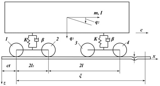
Figure 1.
Railway vehicle design diagram.
Let us choose the following values for the crew as generalized coordinates: —vertical movements of the body, the first and second bogies; —the angles of rotation of the same bodies relative to the main central axis , perpendicular to the vertical plane in which the axis of the track lies; and —the displacement of the center of mass of the system along the axis of the track. Let us denote the deflections of the beam by , and the current ordinates of the geometric irregularity of the unloaded rail by . Let us express the movements of all wheelsets in terms of the specified values (the numbering of wheelsets is given in Figure 1):
where is the bogie base.
Using the Expressions (1), we get
We formulate the differential equations of motion for the railway vehicle under the same assumptions as in [24,26], using Lagrange’s equations of the second kind:
where is the kinetic energy of the system, is the potential energy of the system, is the scattering function, and is the generalized force corresponding to generalized coordinate .
Kinetic energy has a diagonal form:
where are body and bogie weights; are, respectively, the moments of inertia of the body, bogie, and wheelset relative to the main central axis ( is the wheel radius.
The potential compression energy of spring sets is calculated using Clapeyron’s theorem:
where is the spring set stiffness; and are the spring sets’ compression; and is the wheelbase of the railway vehicle.
The scattering function is proportional to the potential energy:
where is the viscous friction coefficient of dampers.
As the generalized forces, we consider the vertical dynamic forces, , acting from the rails on the wheelsets (()). The generalized forces are calculated as the coefficients of the variations in the generalized coordinates in the expressions for the virtual work:
By substituting Expressions (4)—(7) into Equation (3), we obtain the differential equations of the railway vehicle’s oscillations:
The seventh differential equation of the system (8) is the equation of the translational motion of the crew. The third to sixth differential equations of the system (8) are used to determine the forces, ; instead of generalized coordinates, , substitute (2), and, taking into account that , we get (the notation )
Everywhere, the dots indicate the full derivatives of t.
Let us substitute the relation (2) into the first two differential equations of the system (8):
The integration of the differential equations of motion (10) under condition (9) will be carried out in a movable coordinate system, .
Suppose that the periodic irregularities of the rail track are described by the following analytical expressions:
where mm is the depth, m is the unevenness length, and m is the distance between irregularities.
Deterministic irregularities of type (11) are widely used in research and have a rich frequency spectrum [30], in which case the periodic function (11) is decomposed into a Fourier series, which is conveniently represented in a complex form, ,
In the movable coordinate system, the irregularities (11) and (12) are written as follows:
where is the frequency; is the delay of the n-th wheelset from the first; and .
With a numerical solution, the series (13) has a finite number of terms; for the convenience of performing calculations, it is possible to limit the series to 15 terms.
We will look for the solution to the problem in the form (19)
As a result of substituting (14) and (13) in Equations (10) and in conditions (9) recorded in a movable coordinate system, we obtain the following for one term of series (14):
Expressions (15) and (16) must be supplemented by an equation that is solved for a single force, , acting with a frequency, , and applied at the point . Next, using the principle of superposition, we define from all four forces, , and solve a system of six algebraic Equations (15) and (16) to find the deflections of the rail under the four wheelsets, , and amplitudes, .
The numerical solution was made with the following crew parameters:
, and the rail parameters presented in a total of 25 terms of series (13) were taken into account.
In the process of this study, an oscillogram of dynamic support force, , was analyzed in the sets of spring preparation of the first spring preparation during the movement of the bogie; force cooperation on the first drive way the first pair of pairs of bogie and paths (in these boxes was ); the dynamic support of rail servicing, , and other moments, , in the non-stop system coordinates in the family x = 0, 1.5, 3, and 12.5 m (at the beginning, in the middle, the end of the river and the middle of the rail section); and the analogue of the velocity of the and the in the sub-system coordinates in the first row ingress and others parameters at operating speeds of c = 60,100,140, and 180 km/h.
During this study, oscillograms of the dynamic force increments, , in the sets of suspension springs of the first bogie (in the direction of motion) were analyzed, along with the interaction forces, , between the first wheelset of the first bogie and the track (denoted as in the equations).
Additionally, the dynamic increments of rail deflections, , and bending moments, , in the rails were examined in a stationary coordinate system at cross-sections m (at the beginning, middle, and end of the irregularity, as well as at the midpoint of the rail segment). Analogous values, and , were analyzed in a moving coordinate system at the cross-section beneath the first wheelset.
These parameters were studied at vehicle speeds of and km/h. The oscillograms of forces S and S_B match those obtained from solving the problem of vehicle movement on an elastic–viscous foundation. This indicates that the influence of adjacent wheelsets on the displacement of a given wheelset is insignificant.
Under these conditions, the problem of rolling stock and track interaction can be considered as the oscillations of a vehicle moving on inertial elastic–viscous “supports”. However, a definitive conclusion can only be drawn by solving the interaction problem both with and without considering the influence of adjacent wheelsets, as addressed in the following section.
During the calculations, the rail deflections beneath each wheelset were determined as follows:
If the influence of adjacent wheelsets is not taken into account, then the matrix included in (17) is diagonal, and the side coefficients are considered to be zero.
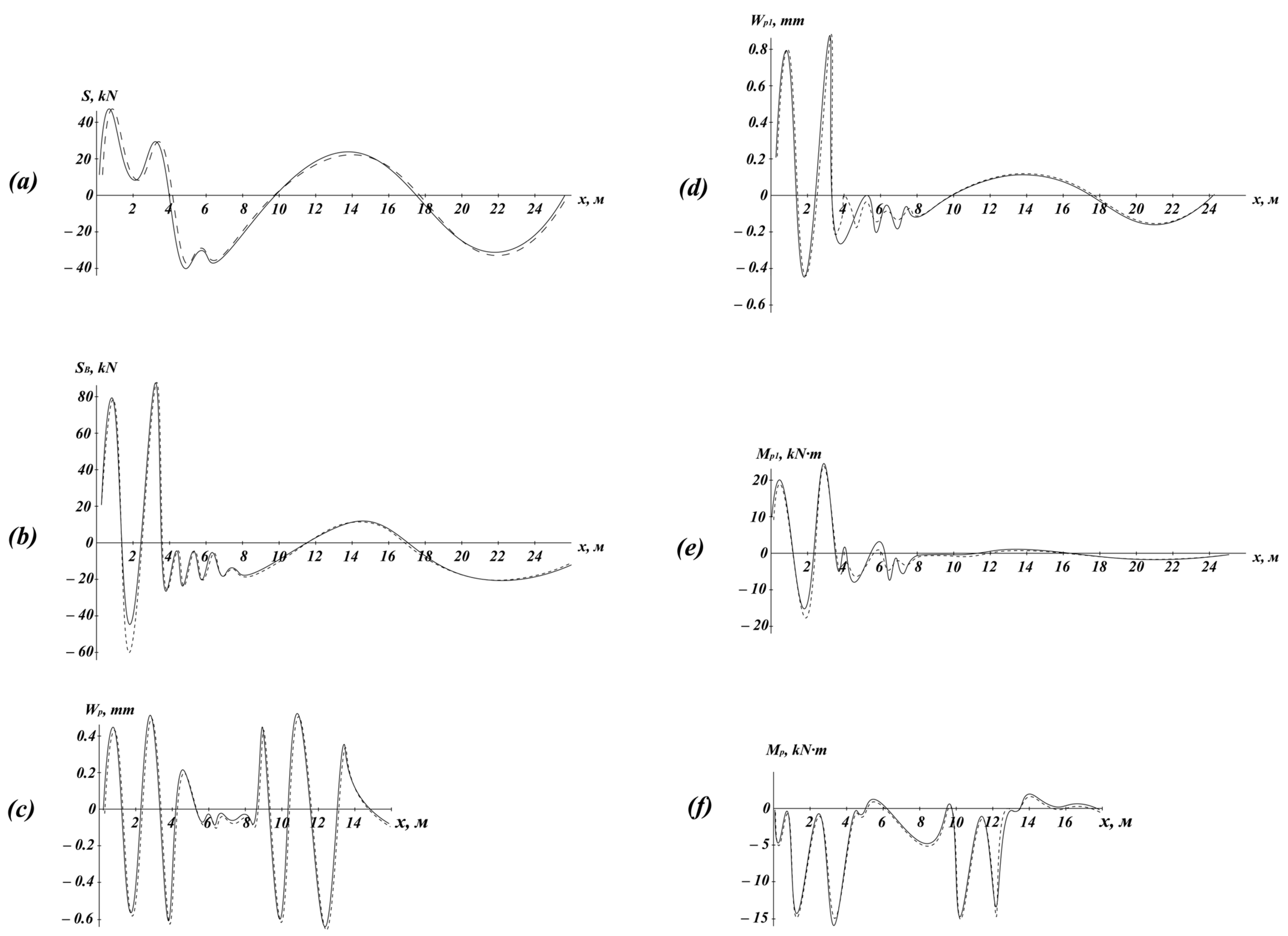
Figure 2 presents the oscillograms of the forces, (Figure 2a) and (Figure 2b); rail deflection, (Figure 2c); and bending moment, (Figure 2d), at the section m, as well as (Figure 2e) and (Figure 2f) at a speed of km/h.
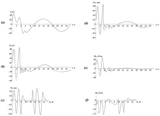
Figure 2.
Oscillograms of forces and bending moment, .
In this figure and all subsequent ones, solid lines represent graphs considering the influence of adjacent wheelsets, while dashed lines depict results without considering this influence.
The graphs indicate that the effect of adjacent wheelsets on the forces in the suspension system is insignificant. However, adjacent wheelsets exert a somewhat greater influence (around 10%) on the interaction forces, , and bending moments, , and an even more significant effect on the amplitude values of rail deflections, (up to 20%).
Similar conclusions were obtained from the analysis of oscillograms of wheelset accelerations and displacements; rail deflections, ; and bending moments, , at other rail sections.
At lower vehicle speeds, the influence of adjacent wheelsets decreases. However, under different railcar parameters, this influence may be more significant.
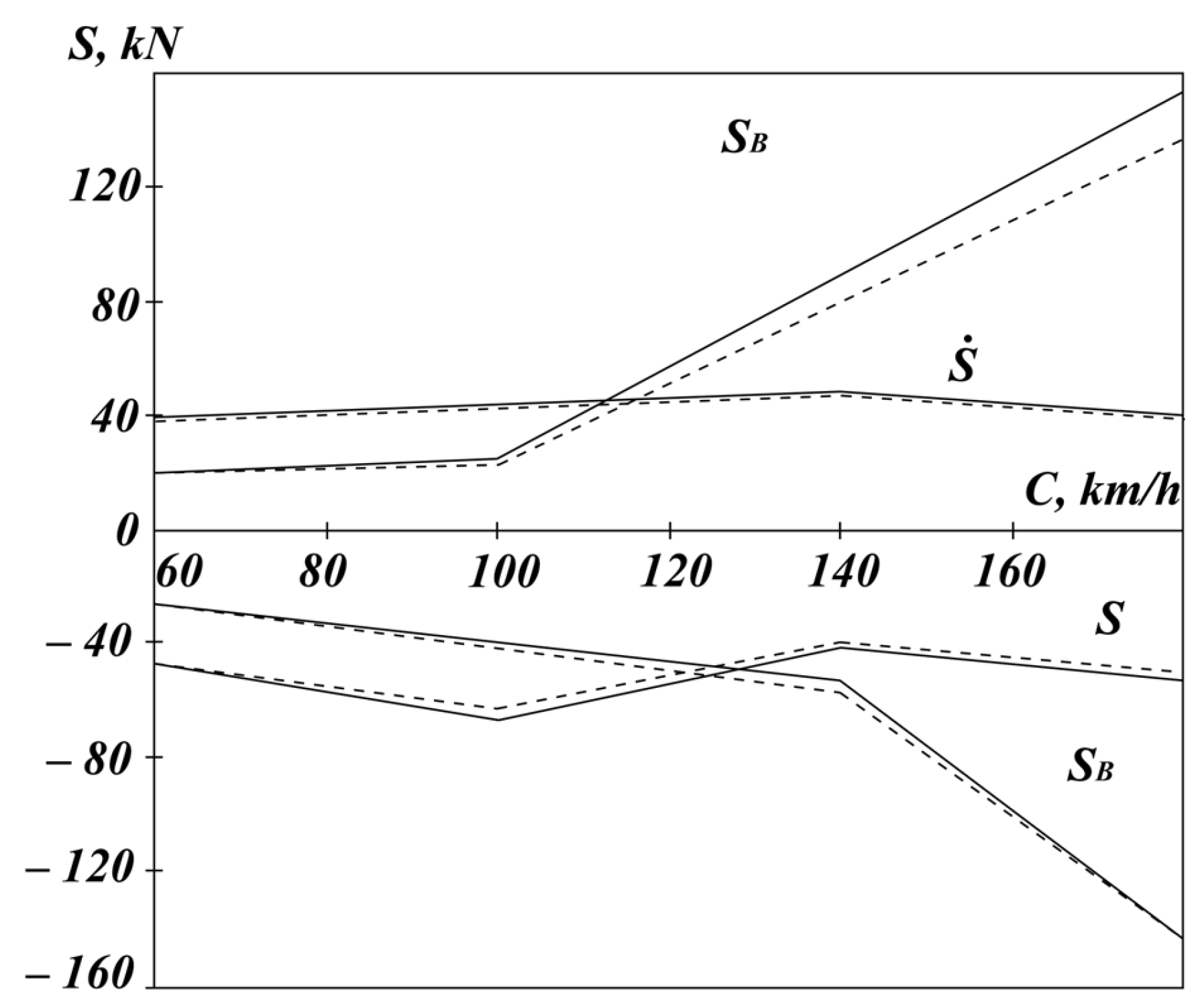
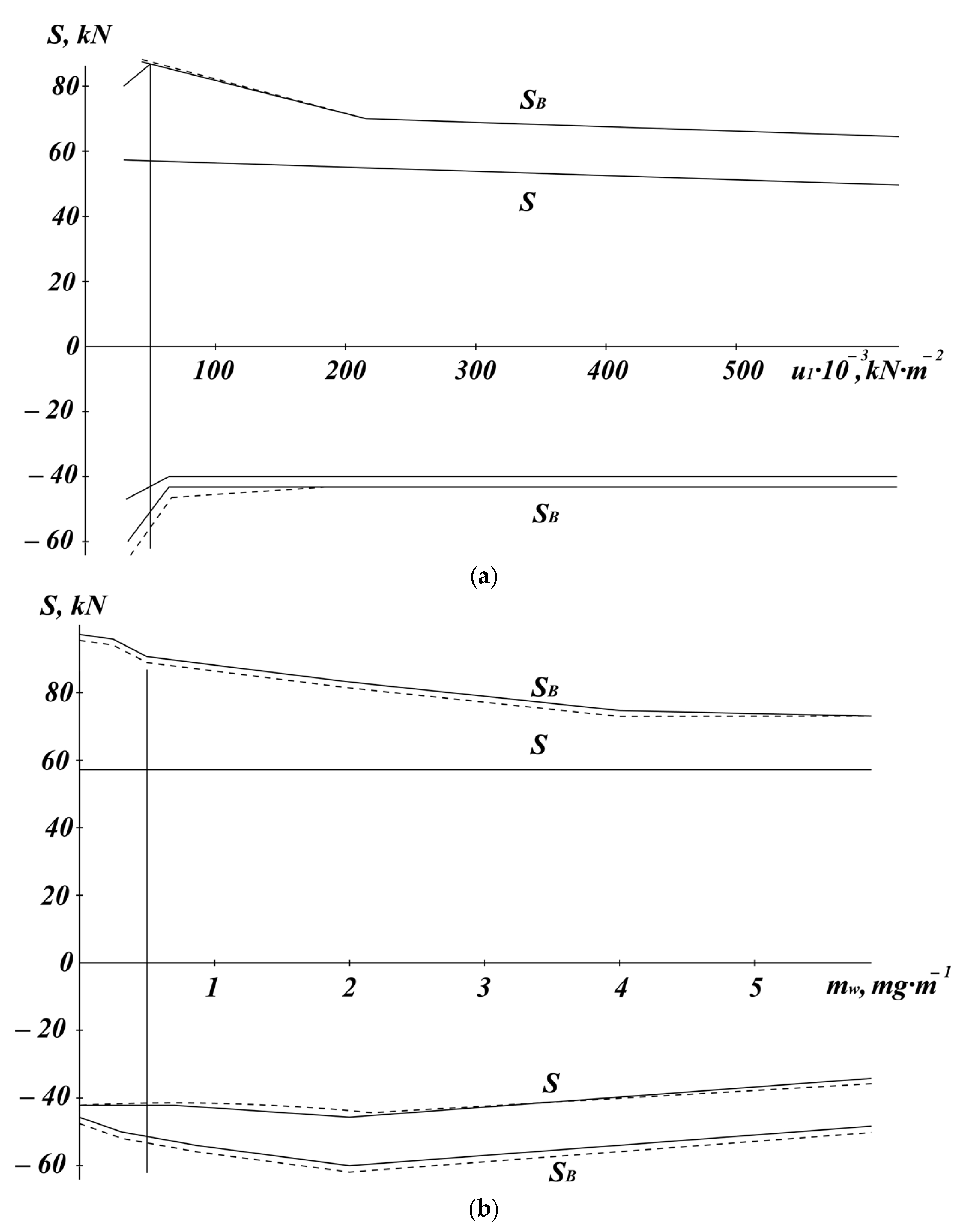
Figure 3 presents graphs showing the dependence of the maximum values of forces and on the vehicle speed. The results indicate that the influence of adjacent wheelsets on the forces and displacements occurring at speeds up to 140 km/h is insignificant and can be neglected. It is important to note that this study considers only perturbations (11) with spectral components containing frequencies up to 20 Hz. This conclusion is obtained at the specified parameters of the rails and the base. Figure 4 shows the graphs of the dependence of the maximum values of the forces and . at km/h from some parameters: base elastic modulus, (Figure 4a), the reduced linear mass of the rails; and the base, (Figure 4b). Vertical lines on these graphs indicate the values corresponding to the initial parameters. As seen from the graphs, the influence of the considered parameters on the forces and is insignificant. The effect of adjacent wheelsets can be neglected across the entire range of parameter variations at the given speed and railcar characteristics.

Figure 3.
Graphs of the dependence of the maximum values of forces and on vehicle speed.
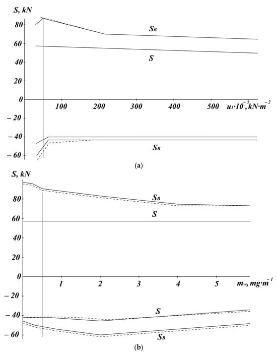
Figure 4.
(a) Graph of the maximum values of forces S and versus the track modulus of elasticity. (b) Graph of the maximum values of forces S and versus the linear mass of the rails.
Thus, the results of this study on the oscillations of a four-axle freight wagon moving along a beam resting on a continuous inertial viscoelastic foundation and on discrete inertial viscoelastic “supports” indicate that the forces acting on the wagon, rail deflections, and bending moments are similar in both cases at speeds up to 140 km/h. Furthermore, the forces arising in the central suspension system remain comparable even at speeds up to 180 km/h. This can be seen from the results of the calculations performed Table 1. This conclusion is supported by Table 2, which presents the values of forces and for the continuum model, considering (first row) and disregarding (second row) the influence of adjacent wheelsets.

Table 1.
Equivalent track parameters derived from inverse frequency response approximation and analytical methods.
Table 2.
The values of forces and for the continuum model, considering (first row) and disregarding (second row) the influence of adjacent wheelsets.
The numerator represents the forces during unloading, while the denominator corresponds to the forces during overloading. The results presented in Table 2 were obtained for an irregularity depth of mm. All other rows in Table 2 show the force values determined from solving the problem of wagon oscillations, considering the track as a system with lumped parameters. Let us represent the rail as a system with lumped parameters and consider it an oscillatory element, where the input is a stationary vertical force, , applied at section , and the output is the deflection at an arbitrary section, x.
In this case, we assume that , meaning that the foundation has only one elastic characteristic. The problem is solved in a stationary coordinate system, i.e., .
The solution represents the frequency response of the considered system. When , it can be interpreted as a stationary linear distributed block: .
We represent it in the following form:
Let us represent the frequency response (18) as
where are the real and imaginary frequency characteristics; and are their magnitude and phase:
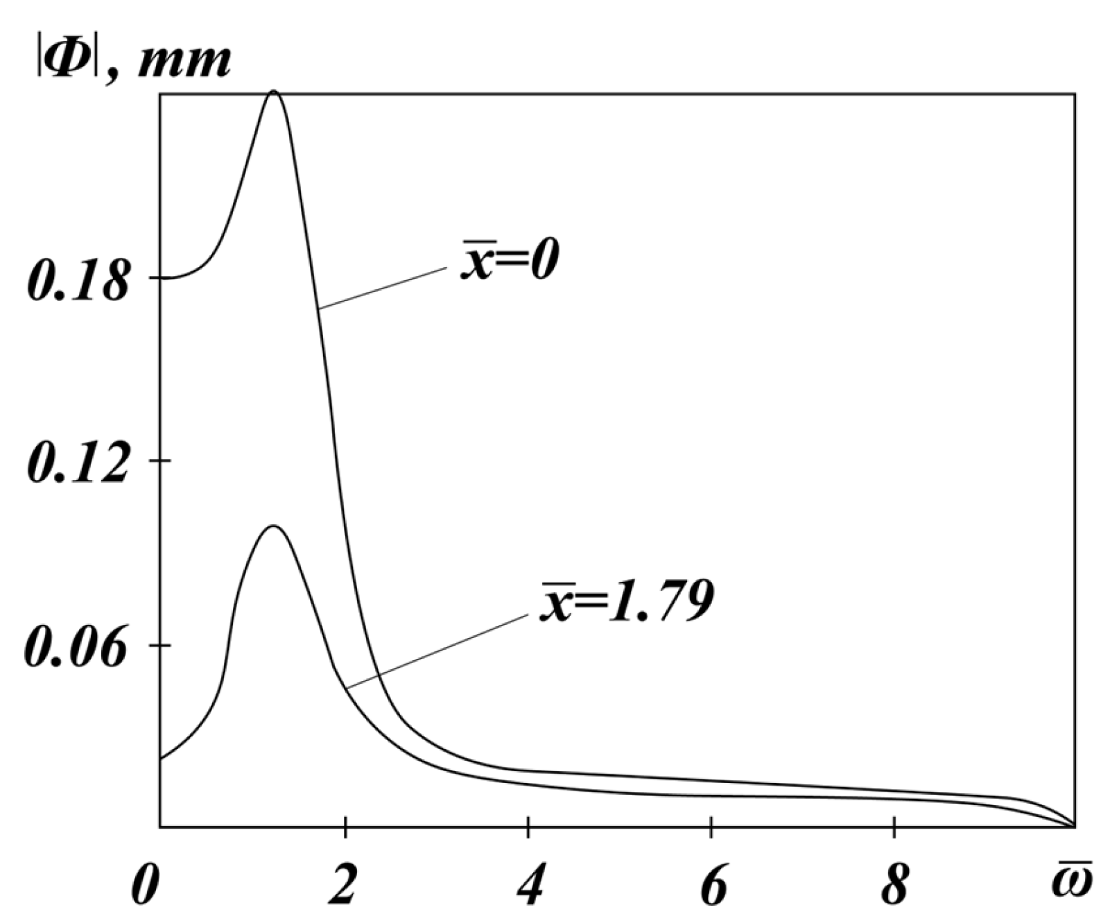
The frequency characteristics (20) are constructed at the accepted values of the initial parameters as follows. Figure 5 shows the graphs for cross-sections and m (the base of the bogie of a wagon; in relative values, at ), depending on the frequency. From the graphs, it can be seen that the modulus of the frequency response has one maximum () at the frequency (we will denote it as ), the value of which increases slightly with an increase in . The value of decreases with increasing , which indicates a weakening of the specified input signal at the output of the system in an arbitrary cross-section, . As is known, the phase-frequency response for the cross-section shows the value of the time delay of the output signal in relation to the input signal. In the section, a spatial delay is added to this lag due to the time of propagation of the signal along the beam.
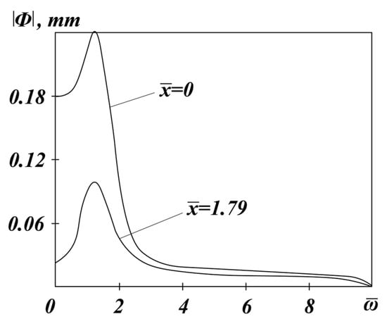
Figure 5.
Graph of the phase response magnitude, |Φ|, as a function of the normalized frequency, .
Let us extract from Equation (20) the block, , which does not depend on the distance, ; thus, let us set in Equation (20). We then obtain the following:
Here, is the system gain coefficient, numerically equal to the static deflection of the beam at the section under the action of a unit force.
We approximate the analytical expression of the block (Equation (21)) with a rational fractional function. The block characterizes an inertial element, which in its properties is similar to a single-frequency oscillator. Therefore, it is natural to represent the frequency response of this block in the following form:
Let us find the inverse frequency response, , which is also referred to as the dynamic stiffness of the system:
The methods for determining the parameters are extremely labor-intensive; a more convenient approach is to replace the frequency response (21) with an equivalent one represented by an n-th degree polynomial, whose coefficients are determined using the least squares method. However, calculations show that this approach is inefficient, and obtaining sufficiently reliable results requires choosing a high system order, n. In this case, the problem can be significantly simplified by directly approximating the inverse frequency responses (23) and (24) with a rational fractional function whose numerator is equal to one. Let us demonstrate this using an example with and .
Using the least squares method, we will construct the squares of the differences between the real and imaginary parts of the given and approximated inverse frequency responses at some points of the frequency range.
And minimize them . We get two systems of algebraic equations:
From the above equations, we will determine parameter .
Let us consider the obtained results. In the first case, satisfactory results are achieved for and , and in the reduced frequency range, the fourth- and third-degree polynomials (23) almost completely match the given inverse frequency response. The second-degree polynomial shows poorer agreement with the inverse frequency response of the given system.
The numerical values of the parameters obtained through calculations based on inverse frequency response characteristics, obtained as a result of calculations using the inverse frequency responses, are presented in the first six rows of Table 1. All values of parameter should be multiplied by and those of by . The results presented in rows 7 to 12 of Table 1 are explained below.
Thus, the considered continuous system with output at the cross-section (block ) and the discrete system with the parameters determined above have practically identical frequency characteristics over a fairly wide frequency range. In the range of , a third-degree polynomial is sufficient for the inverse frequency response. In the range of , acceptable results are obtained even with a second-degree polynomial.
It is worth noting that, in this case, parameters have specific physical meaning—corresponding to the equivalent mass, viscous damping coefficient, and stiffness, respectively. This implies that the railcar is positioned on inertial viscoelastic supports, and the track is modeled in its simplest form—as a single degree-of-freedom system.
The determination of the reduced track parameters has been the subject of numerous studies, and various methods have been proposed for their estimation. V.A. Lazaryan developed [23] an efficient approximate method based on the Shakhunyants hypothesis [1], according to which the dynamic elastic line of the beam is replaced with a quasi-static one (under the action of a moving constant force). Then, the kinetic, , and potential, , energies of the beam are equated to the kinetic, , and potential, , energies of the equivalent system.
We will use the expression for the elastic line of a beam lying on a continuous viscoelastic foundation with a single characteristic, , and loaded with a constant force, , for the case
Then,
where is the mass distributed along the length of the beam and the base; and are the rotating mass and rigidity; and is the beam deflection in section . Having performed the calculations, we get .
As for the viscosity parameter, considering the dissipation function to be proportional to the potential energy of a system with proportionality coefficients, —in case of deformation of the bending of the beam; and —in case of compression deformation of the base—we express the given coefficient of viscous friction in the form of . If we consider that , where and are the stiffness and coefficient of viscous friction of the dampers of the crew spring suspension, then we will get the final formulas of this method of reducing the base parameters:
Taking in the expression for , that (friction in the beam is neglected), we get . Then,
Another approach is based on selecting parameters and , such that the frequency characteristics of the system with one degree of freedom and the system with distributed parameters are close. It is recommended to choose the reduced parameters based on the condition of matching the real, , and imaginary, parts of the frequency characteristics at the peak of the frequency characteristic module and at . Let and (21) be known for the continuous model at frequency , where the maximum of the frequency response occurs. For the system with one degree of freedom,
If we equate and , we obtain and , where ; from this, . However, since is selected based on other conditions, this equality may not hold. Therefore, it is better to select the reduced parameters based on other conditions. For example, we can impose the condition of matching the natural frequencies of the free vibrations of the discrete system, , and the undamped vibrations of the beam, . The reduced stiffness, , is chosen based on the condition of equal static deflections of the beam under force and the discrete system, i.e., denominator of expression for , which coincides with (28). Then, from the condition , it follows that . Now, if we equate the maximum ordinates of the frequency response function, we obtain , from which we can find
All the formulas above were derived for the case of a stationary force (). The influence of the force’s velocity on the system’s frequency characteristics, as noted earlier, is negligible at the existing speeds of railway vehicles. Nevertheless, let us determine the reduced parameters by taking into account the force’s velocity. For the continuous system, let the frequency, , and the maximum of the frequency response function, , be known at some velocity, . Let and . From this, we can find that
Calculations were performed according to Formulas (28)–(32), and the reduced parameters were found for all five methods considered. The results are summarized in Table 1 (lines 7–11).
From the analysis of the data in Table 1, it can be seen that, in all variants (lines 7–11), the reduced stiffness is the same; when approximating the inverse frequency characteristic in the range of , it differs by only 2.5%, and in the range of , it is 28% smaller (for ). The values of the reduced viscous friction coefficient are close to each other in variants ; in the eighth variant, it is 25% lower than the previous ones; and in the third, it is 68% higher. In the seventh variant, its numerical value is 6.5 times greater than in the tenth: it is extremely overestimated. The reduced mass, calculated using Formula (31), is 32% greater than the one computed by the approximation method of the inverse frequency characteristic (26) in the range of 0–1.5 (line 6) and 68% greater in the range of 0–3 (line 3); the difference in the reduced mass in the tenth variant from the one obtained by the method based on the equality of the kinetic energies of the distributed and reduced systems (28) and (29) is 26%.
In the frequency range of , the agreement of all characteristics is good; at higher frequencies, there is a divergence, especially between the real frequency characteristics. This divergence is explained by the overestimated value of the parameter Mg. Therefore, to determine the reduced parameters of the path based on the known distributed parameters, it is recommended to use Formula (31) for investigations in the low-frequency range, not exceeding , and for higher frequencies (up to ), the following formulas:
The parameters calculated using Formula (33) are presented in line 12 of Table 1. The conducted study makes it possible to determine the reduced parameters of the track without considering the influence of the adjacent wheelset. The results of solving the problem of wagon vibrations are given in Table 2. If the influence of the adjacent wheelset is to be taken into account, it is necessary to consider the frequency characteristics (19) and (20) after isolating the block.
where .
After carrying out the corresponding derivations, we obtain
Let us consider the frequency characteristic (35); and the real and imaginary frequency characteristics, and , for the section . This characteristic can be approximated in various ways over different segments of the frequency range. In the range of for fixed values of , the frequency characteristic, , is approximated by a polynomial:
For example, if we take , then, as before, we construct the squares of the differences between the given (25) and the target (36) frequency characteristics separately for the real and imaginary parts. This leads to systems of algebraic equations analogous to (26), where the coefficients are replaced with , and in (27) are replaced with . The numerical values of the parameters were obtained as follows: .
The frequency range of is of greatest practical interest, as the natural frequencies of wagon vibrations are significantly lower than the upper limit of this range. Therefore, in subsequent calculations, we will consider only this range and assume that the system’s frequency characteristic is approximated by expressions (23), (34), and (36).
Thus, the frequency characteristic of the considered system is represented as the product (34) of the frequency characteristics of two blocks, one of which determines the output signal at the section (block ); and the other—block —depends on the spatial coordinate, .
If several forces act on the rail, then the deflection, , under the force, , with the abscissa, , is equal to
Equation (37), taking into account (23) and (36), can be written as
Since the block must be inertial, in the fractional–rational function (38), the degree of the polynomial in the denominator must be higher than that in the numerator, i.e., , which is assumed in the calculation.
In expression (38), the coefficients are given additional indices, , indicating their dependence on the abscissas, and . Obviously, since , and also for , and for .
There is no fundamental difficulty in considering the case when the asymmetry of the function must be taken into account. In this case, the matrix of coefficients, , is not symmetric with respect to the indices, , thus leading to an increase in the amount of computation.
By summing Equation (38) over the index, , one can obtain an expression for the total deflection of the rail at the section with abscissa, , under the action of all forces.
Or
Expression (40) allows us to write the following differential relationships between the inputs, , and the outputs, :
Thus, the system with distributed parameters is reduced to a system with lumped parameters (41).
In conclusion of the conducted study, let us determine the equivalent (reduced) parameters of the rail during its vibrations in the horizontal plane. In this case, two maxima of the frequency response function (FRF) occur in the absence of damping. However, if damping in the foundation is taken into account, the second maximum disappears, and the FRF of the system, as in the case of vertical vibrations, becomes close to that of an oscillator. Therefore, we use Formula (33) to determine the equivalent parameters of the track in the horizontal plane; the resulting values for the initial parameters are () .
To determine , Formulas (33) and (31) were used. The equivalent stiffness, , was determined based on the displacements of the rail’s bending center. If it is determined based on the compression of the rail head, then .
Next, we consider the planar vibrations of a railcar moving along a track modeled as a system with lumped parameters. We will use the results presented analytically at the beginning of the article and in Table 1, where the rail is also represented as a system with lumped parameters.
We write the differential relationship between the forces from one bogie and the deflections of the rail under the first and second wheelsets of the first bogie (see Figure 1), neglecting the deflections under the wheelsets of one bogie caused by the interaction forces of the wheelsets of the other bogie and the rail (41):
And similar expressions are used for the rest of the deflections.
In Equation (42), dots denote time derivatives.
Substituting the expressions for deflections (1) into (42), after differentiating them beforehand, we obtain a system of differential equations. By performing simple transformations—pairwise addition and subtraction of the equations—we arrive at the following system of differential equations:
The following notations are introduced here:
The differential equations of the wagon oscillations (8) can be written in the following form (excluding the cyclic coordinate):
Equation (45) can be derived directly from D’Alembert’s principle [24]. In these equations, are the forces arising in the spring assemblies of the central suspension system.
For viscous damping, they are given by ; and for Coulomb friction dampers, they are given by , where is the Coulomb friction force.
The inelastic component of the forces, (denoted as ), is expressed by an analytical function that approximates the “signature” behavior but is itself a smooth function.
where is a coefficient characterizing the steepness of the characteristic slope at low displacement velocities. When using expressions (46), the integration of the differential equations proceeds without any peculiarities.
From Equations (43) and (45), we eliminate the forces, (Equation (44)). As a result, we obtain the following system of differential equations:
To integrate Equation (47), the time derivatives of the function are required. These will be calculated as derivatives of the composite function (46):
Differentiating the resulting expression as a product, we find
The system of differential Equation (47) can be integrated. It is a system of six equations of the 24th order. The results of its integration, considering only the real part of the frequency characteristic in expression (36) (; the parameters are taken from the fourth row of Table 1), are presented in the third row of Table 2.
From the comparison of the amplitude values of the spring suspension forces, , and the interaction forces, , in the third and first cases, it is evident that all forces are greater when Coulomb friction dampers are used. In the case where the influence of the adjacent wheelset is neglected, all should be set in system (47). Then, the system order is reduced to 20, and the right-hand sides of the third and fifth equations no longer contain the time derivatives of the forces, . The corresponding results are presented in the fourth row of Table 2, from which it can be seen that adjacent wheelsets under Coulomb friction damping have a greater effect on all forces (up to 21%) compared to viscous damping (the discrepancy does not exceed 10%, and only in the interaction forces).
The influence of the number of terms in polynomial (23), which approximates block , can be assessed by comparing the data in the fourth row of Table 2 with those in the fifth row, which presents the results of integrating system (47), with and parameters taken from the sixth row of Table 1. The transition from a fourth-degree polynomial (23) to a second-degree polynomial has practically no effect on the results (the error does not exceed 1.3%). Thus, a second-degree polynomial can be used to approximate block .
The fifth case was also calculated for viscous friction dampers (sixth row); the forces, and , were found to be smaller with viscous damping across the entire speed range considered.
If we compare the results given in the second and sixth rows of Table 2—that is, results obtained for the same problem but solved using different approaches (in the frequency domain—second case; and in the time domain with prior approximation of block by a second-degree polynomial—sixth case), we observe a very good match (only in one case does the discrepancy reach 6%, while in all others, it is significantly smaller).
In all subsequent cases (rows 7–11), the influence of the adjacent wheelset is not taken into account, and the block is approximated by a second-degree polynomial, meaning that the given track parameters are considered. The seventh, eighth, and ninth cases correspond to the same-numbered cases in Table 1. In the seventh and eighth cases, and were calculated based on the equality of the kinetic and potential energies of the distributed and reduced systems. However, in the seventh case, track damping was overestimated. The high damping value led to a noticeable decrease in the magnitude of all forces at high speeds (compared to the second case: the suspension forces decreased by up to 19%, and the interaction forces by up to 31% at a speed of 180 km/h). Without considering damping in the beam (eighth case), the forces are close to those obtained from the continuous model without accounting for the influence of adjacent wheelsets (second case). In the ninth case, the results are given for the equivalent parameters obtained by comparing the frequency characteristics of the distributed and discrete systems.
The differences from the eighth case are minor: at a speed of 180 km/h, the forces, , decreased by 4%, and by 7%. Therefore, all the considered methods of reducing the distributed track parameters to lumped parameters yield similar results in terms of the magnitude of the forces acting on the wagon body and wheelsets, except in cases with excessively high friction. In the last two cases, the tenth and eleventh, the influence of the inertial properties of the track on the considered dynamic characteristics of the railcar is investigated. In case 10, the parameters from case 9 are used, but is assumed to be zero. The forces in the suspension system change insignificantly (by no more than 6%), while the interaction forces for the non-inertial track are 8% higher than those for the inertial track (at speeds of 140–180 km/h). Finally, let us compare cases 5 and 11, which allow us to assess the impact of the inertial properties of the track when Coulomb friction dampers are used in the railcar’s suspension system. The forces, S, vary less in this case (differences do not exceed 8%), as in the linear problem, compared to the interaction forces, which increase sharply for the non-inertial track (from 21% at km/h to 96% at km/h).
This leads to the conclusion that it is essential to take into account the inertial properties of the track, especially when analyzing railcar vibrations in a nonlinear setting.
3. Experimental Setup
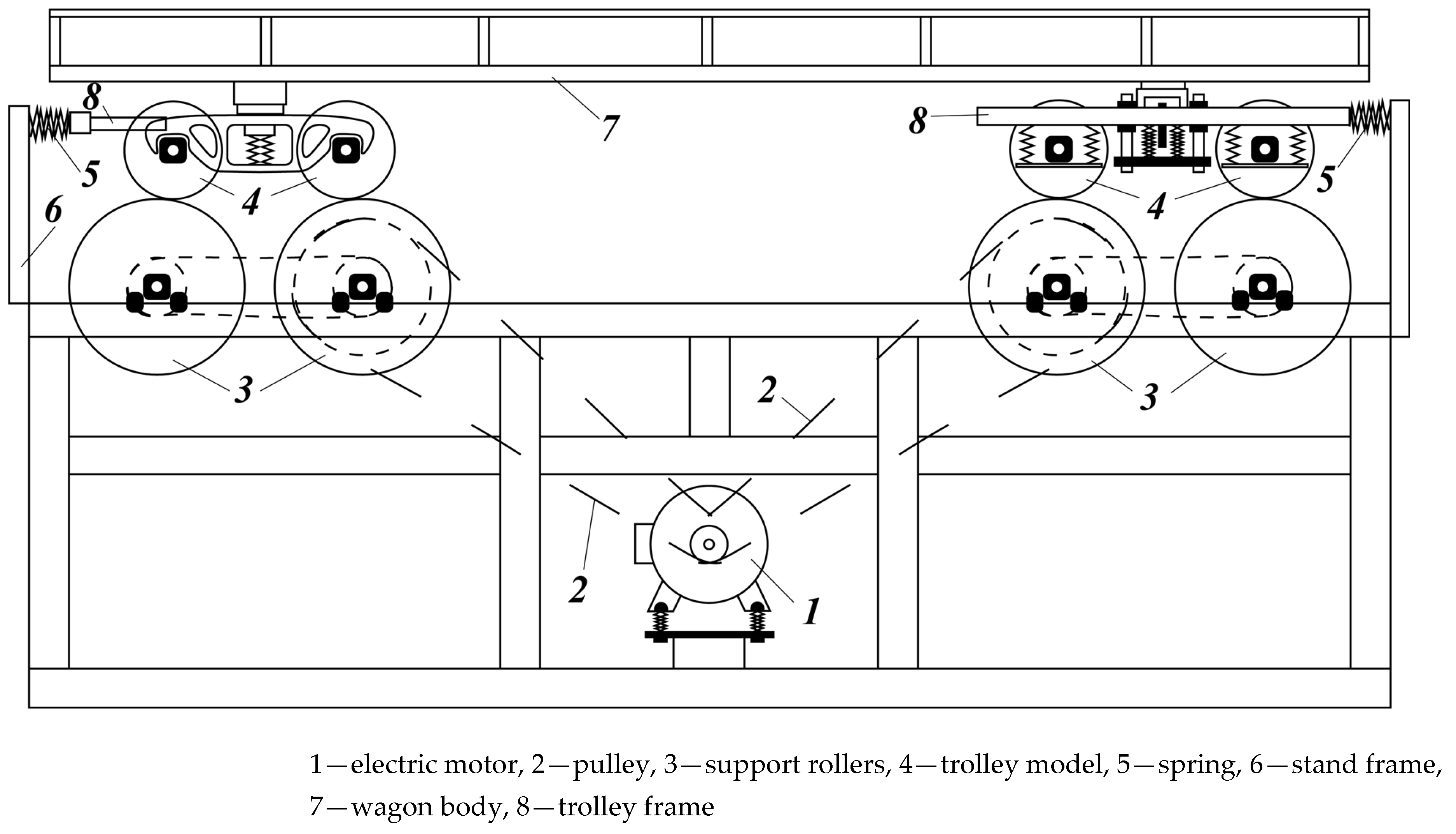
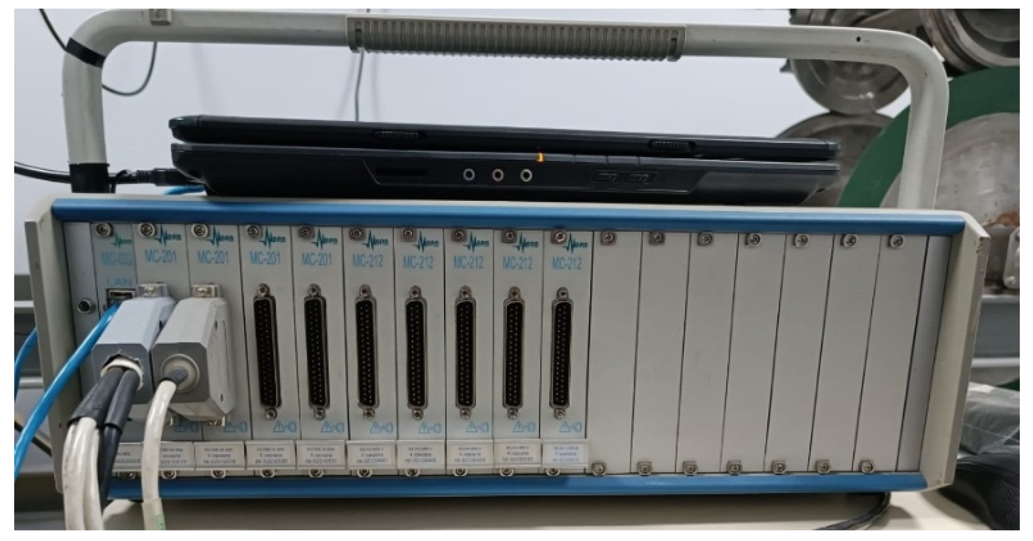
The experimental part of this study was carried out using a roller bench, the schematic of which is shown in Figure 6. The bench’s design is protected by a patent [25]. The construction of the stand allows for the replacement of the tested bogie models, thereby enabling tests for various types of railway vehicles under simulated operating conditions. The adjustment mechanism for the longitudinal displacement of the bogie models on the roller test stand is shown in Figure 7. The roller bench includes a measuring and computing complex MIC-036 (Figure 8), which is designed for collecting, converting, recording, processing, transmitting, and displaying information from sensors and measuring transducers. It functions as a component of automatic and automated multichannel measurement systems used for recording and processing diagnostic test results of various railway vehicle models.
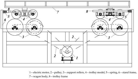
Figure 6.
Diagram of a roller test bench for the study of the dynamic characteristics of railway carriage models.
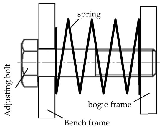
Figure 7.
Diagram of the longitudinal adjustment of bogie models using an adjustment bolt.
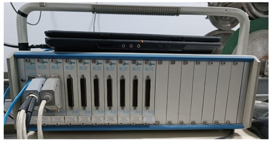
Figure 8.
Measuring and computing complex MIC-036.
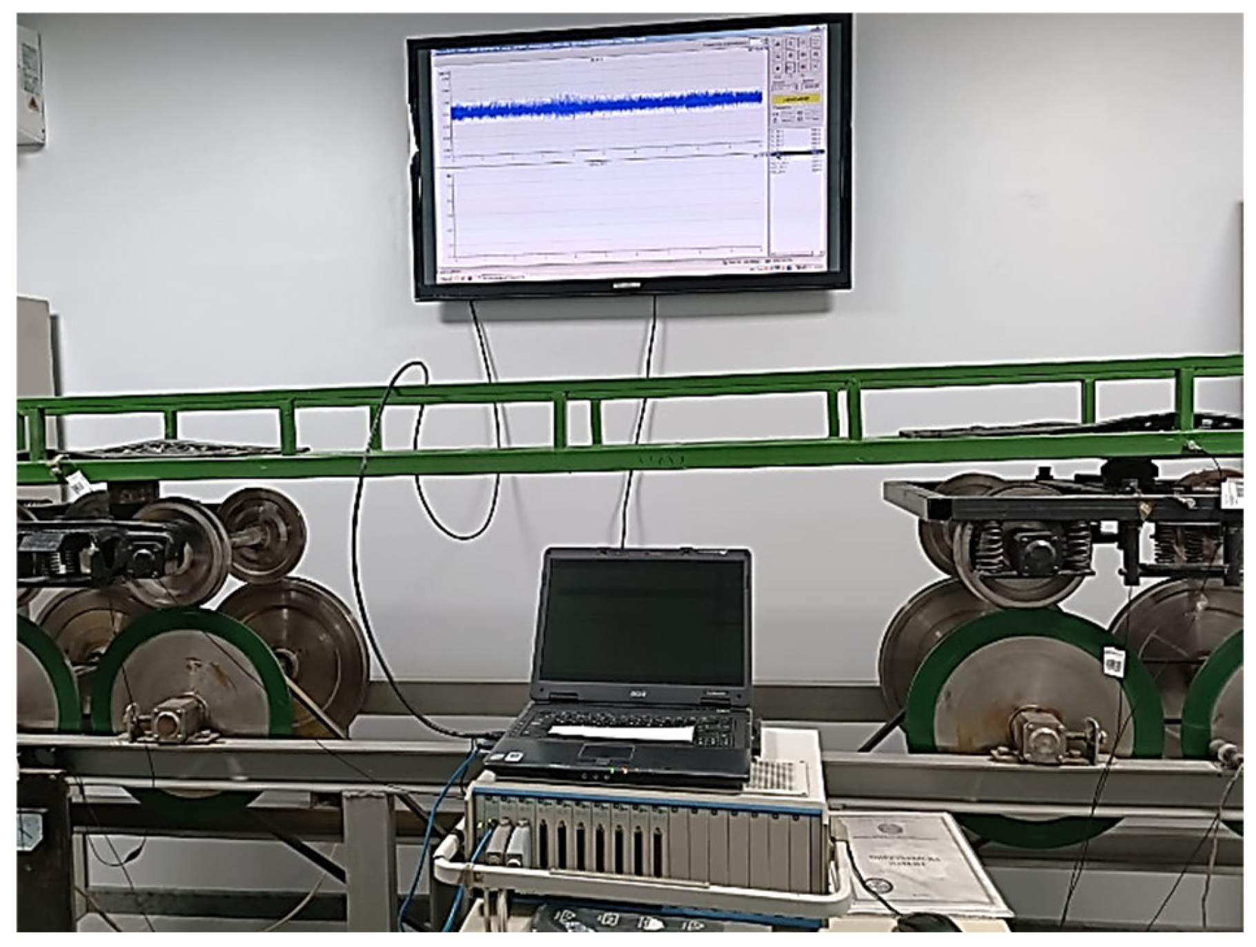
The bench operates as follows: The electric motor 1 (Figure 6) drives the rollers 3 of the stand through pulleys 2 and a V-belt transmission. These rollers, in turn, rotate the wheelsets 4 of the bogies resting on them, thus simulating the motion of railway vehicles along a real track. The wagon 7 rests on the bogies 4. Longitudinal forces are simulated using springs 5, which are welded on one side to the bench frame 6 and on the other to the bogie frame 8. Longitudinal displacement is adjusted by means of a regulating bolt (Figure 7). The rollers of the bench feature various irregularities simulating joint imperfections and track defects, while the interchangeable wheelsets are equipped with irregularities that mimic different operational defects of railway vehicle wheelsets. This setup enables a wide range of dynamic bench tests of railway vehicle models to be conducted under laboratory conditions. Vibration and strain sensors are mounted on the car body frame, bogie components, and axlebox assemblies to record diagnostic parameters (Figure 9). Signals from these sensors are captured and processed by the MIC-036 measuring and computing system and displayed on a computer or laptop screen. The MIC-036 measuring and computing system, which is part of the bench, is a combination of hardware and software tools that not only implement a standard digital signal processing scheme but also perform the entire measurement process—from receiving electrical signals from primary transducers to outputting controlled process parameters in physical units.
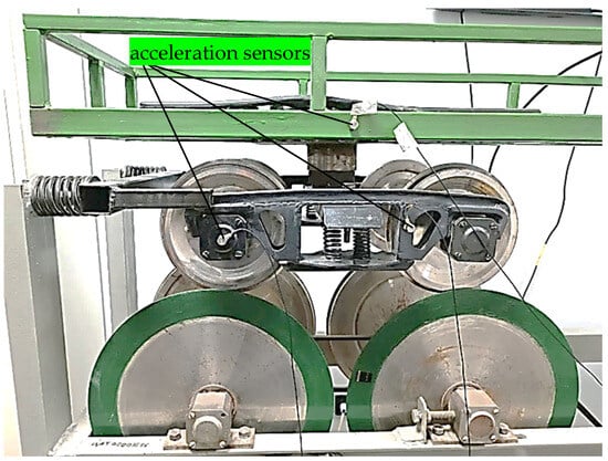
Figure 9.
Model of a wagon bogie with acceleration sensors.
The MIC measuring and computing complexes form the basis of the measurement system of the bench, providing data acquisition, signal conversion, and processing from sensors. These complexes can also be integrated into more advanced and branched information-measurement systems for solving a wide range of tasks (e.g., during field tests of transport equipment).
4. Experimental Validation
The complex includes standard software called Recorder (nppmera.ru), which performs configuration of the system, diagnostics of module functionality, setting of measurement ranges, and calibration and adjustment of the measurement channels, as well as presenting the measured parameters to the user in terms of their physical values (Figure 10).
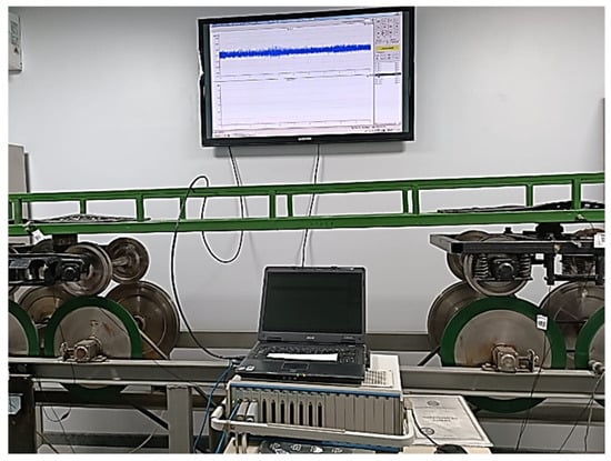
Figure 10.
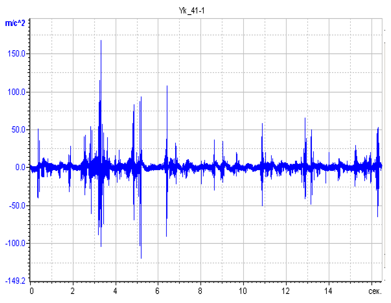
Measurement of axlebox accelerations on the roller bench.
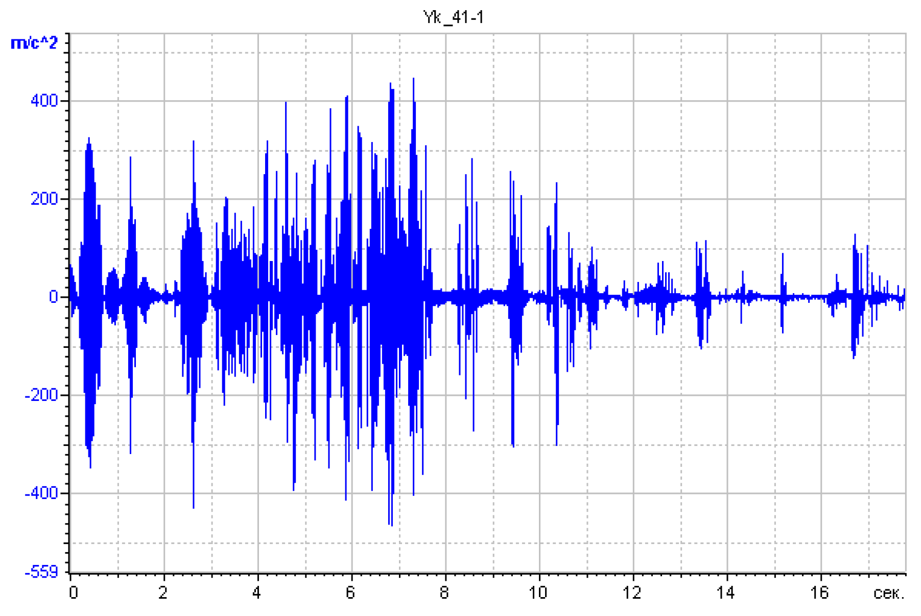
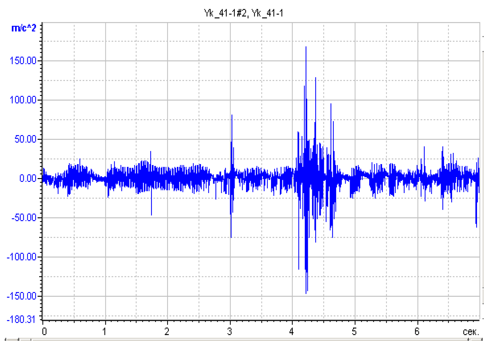
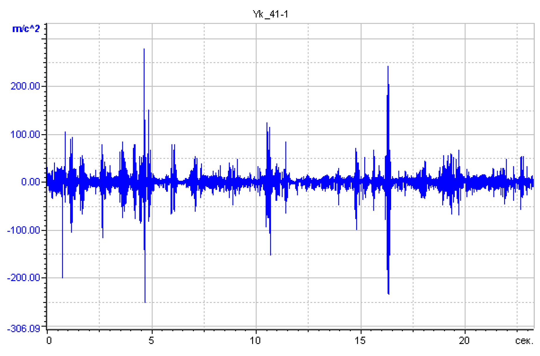
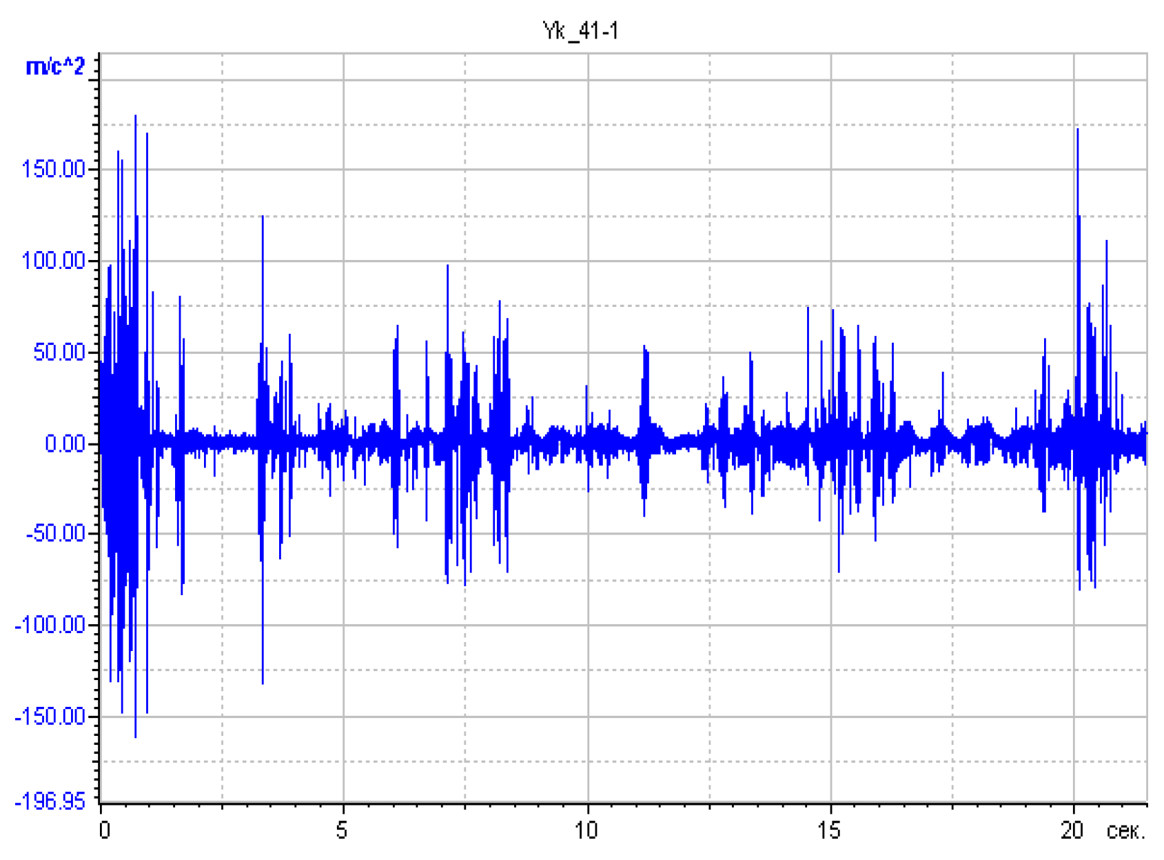
The graphs of acceleration measurements for the sprung and unsprung parts of the freight car models are shown in Figure 11, Figure 12, Figure 13, Figure 14 and Figure 15.

Figure 11.
Graph of the vertical acceleration response of the unsprung masses in the bogie model.
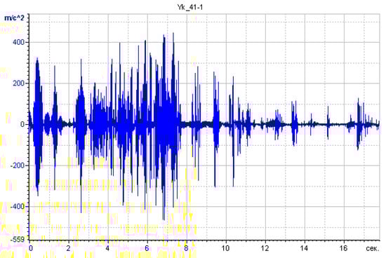
Figure 12.
Graph of the horizontal acceleration response of the unsprung masses in the bogie model.
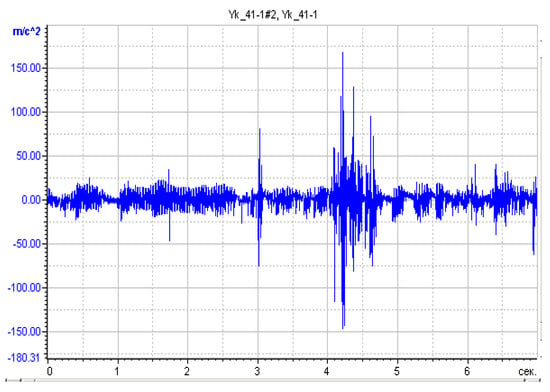
Figure 13.
Vertical acceleration response of the sprung masses of the bogie model.
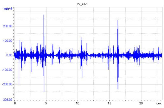
Figure 14.
Graph of horizontal accelerations of the sprung masses of the bogie model.

Figure 15.
Vertical acceleration response of the wagon frame.
Analyzing the obtained graphs (Figure 11, Figure 12, Figure 13, Figure 14 and Figure 15), the following conclusions can be made: modeling the motion of the wagon bogie model at different speeds shows that the suspension components of the bogie practically do not move. The body oscillations occur mainly due to its elastic properties, as evidenced by the recorded displacements of the unsprung beam of the bogie. In other words, the oscillations recorded on the oscillograms result from the bending vibrations of the body, acting as an elastic beam resting on two supports.
The frequency of body oscillations, determined from the obtained accelerations, is in the range of 6–7 Hz. When simulating higher speeds of the freight car bogie model, body oscillations occur due to the movements of the suspension system, which are aperiodic and quickly damped. Additionally, during modeling, periodic oscillations of the body on the suspension system are observed, occurring at nearly all speeds, with a frequency close to the natural frequency of oscillations. Due to the small magnitude of the static deflection and insufficient damping of the vibrations, the amplitude of acceleration increases with speed, and the oscillations slowly decay.
5. Conclusions and Recommendations
The conducted studies and obtained results allow the following main conclusions and recommendations to be formulated:
- A study of the vibrations of a wagon moving along an inertial elastic–viscous track was carried out in a linear formulation; dynamic additions to the forces in the spring suspension sets, interaction forces, rail deflections, and bending moments in the rails were analyzed in both moving and stationary coordinate systems. It was established that the influence of the neighboring wheelset affects the interaction forces and bending moments (by approximately 10%) and, to a greater extent, the rail deflections (up to 20%). This conclusion holds true for the speed range of 60–180 km/h and disturbances with spectral frequencies up to 20 Hz.
- Existing methods and new approaches for representing the rail as a system with concentrated parameters were considered and developed. For this purpose, the frequency characteristic of the studied system is represented as the product of two blocks, one of which defines the output signal at the same section where the force is applied, while the other depends on the spatial coordinate. The real and imaginary frequency characteristics of both blocks were constructed, and their approximation by polynomials was carried out using the least squares method within a frequency range exceeding the natural frequencies of the wagon vibrations.
- The frequency characteristic of the block determining the output signal at the same section where the force is applied can, in the first approximation, be represented by a second-degree polynomial; the coefficients of this polynomial correspond to the reduced mass, stiffness, and coefficient of viscous friction.
- It was established that, at the existing wagon speeds, the reduced parameters of the track can be determined from the frequency characteristic of the track obtained under a stationary force.
- Numerical values of the reduced track parameters in the vertical and horizontal planes were determined.
- The developed method for representing the rail as a system with concentrated parameters allowed for this study of the planar vibrations of a wagon moving along an inertial elastoviscous track, taking into account the influence of the neighboring wheelset in the nonlinear formulation. When accounting for Coulomb friction dampers in the wagon’s suspension, the forces acting on the body and wheelsets were found to be larger than those with viscous friction dampers.
- When solving the problem in the nonlinear formulation, the influence of the neighboring wheelset affects the forces arising in the suspension spring assemblies of the body to a greater extent (up to 21%).
- An overestimated value of friction in the track leads to a significant reduction in all forces (in the suspension—up to 19%; interaction forces—up to 31%) at high speeds.
- It was established that the inertial properties of the track must be taken into account when studying the vibrations of wagons, especially in the nonlinear formulation. The forces in the suspension for a non-inertial track are 6% larger, and the interaction forces are 8% larger compared to the inertial track with viscous friction dampers, and 8% and 96% larger, respectively, with Coulomb friction dampers.
- The results obtained through the roller stand simulations at varying speeds of the freight car model show that the suspension spring assemblies of the truck hardly move. The body vibrations, occurring due to its elastic properties, have a frequency of 6–7 Hz. Due to the small magnitude of static deflection and insufficient damping of the vibrations, the amplitude of the accelerations increases with speed, while the vibrations gradually decay.
Author Contributions
Study conception and design, V.G.S. and N.M.M.; data collection, A.A.M. and S.T.A.; analysis and interpretation of results, N.V.I. and J.S.M.; draft manuscript preparation, G.T.Y. All authors have read and agreed to the published version of the manuscript.
Funding
This research was conducted as part of the preparation for the grant funding project on scientific and (or) scientific–technical projects for 2024–2026, AP23487831, “Modeling Track Irregularities for Investigating the Dynamic Qualities of the Innovative Rolling Stock Based on Theoretical and Experimental Studies”.
Institutional Review Board Statement
Not applicable.
Informed Consent Statement
Not applicable.
Data Availability Statement
The data presented in this study are available in the article.
Conflicts of Interest
The authors declare no conflicts of interest.
References
- Queguineur, A.; Daareyni, A.; Mokhtarian, H.; Isakov, M.; Rook, R.; Ya, W.; Goulas, C.; Hascoët, J.Y.; Ituarte, I.F. Digital design and manufacturing of a railway bogie demonstrator via multi-material wire arc directed energy deposition. Int. J. Adv. Manuf. Technol. 2025, 136, 5281–5303. [Google Scholar] [CrossRef]
- European Commission. Railway Innovation in the 21st Century. Horizon Europe NCP Portal. 2024. Available online: https://horizoneuropencpportal.eu/sites/default/files/2024-06/cer-railway-innovation-in-the-21st-century-2024.pdf (accessed on 20 January 2025).
- Kalker, J.J. On the Rolling of Two Elastic Bodies in the Presence of Dry Friction. Ph.D. Thesis, Delft Technological University, Delft, The Netherlands, 1967. [Google Scholar]
- Triple, E. Innovations in Railway Construction Materials. 2024. Available online: https://eeesa.com/en/railway-innovations-at-triple-e-2024/ (accessed on 20 January 2025).
- Kalker, J.J. Three Dimensional Elastic Bodies in Rolling Contact, 1st ed.; Kluwer: Dordrecht, The Netherlands, 1990. [Google Scholar]
- McClanachan, M. An Investigation of the Effect of Bogie and Wagon Pitch Associated with Longitudinal Train Dynamics. In The Dynamics of Vehicles on Roads and on Tracks-Vehicle System Dynamics Supplement 33; McClanachan, M., Cole, C., Roach, D., Scown, B., Eds.; Swets & Zeitlinger: Amsterdam, The Netherlands, 1999; pp. 374–385. [Google Scholar]
- Kooban, F.; Radlińska, A.; Mousapour, R.; Saraei, M. Advanced technology in railway track monitoring using the GPR technique: A review. arXiv 2025, arXiv:2501.11132. [Google Scholar] [CrossRef]
- Ayasse, J.B.; Chollet, H. Determination of the wheel rail contact patch for semiHertzian conditions. Veh. Syst. Dyn. 2005, 43, 161–172. [Google Scholar] [CrossRef]
- Muller, L.; Witt, T. TRAIN—A Computer Model for the Simulation of Longitudinal Dynamics in Trains. In Conference on Railway Engineering; Institution of Engineers: Rockhampton, Australia, 1998; pp. 181–186. [Google Scholar]
- Science Direct. Advancing railway sustainability: Strategic integration of circular economy principles in ballasted track systems. J. Clean. Prod. 2025, 490, 44713. [Google Scholar]
- Research Gate. Innovative Trends in Railway Condition Monitoring. 2025. Available online: https://www.researchgate.net/publication/377580179_Innovative_Trends_in_Railway_Condition_Monitoring (accessed on 21 January 2025).
- Polach, O. Creep forces in simulations of traction vehicles running on adhesion limit. In Proceedings of the Sixth International Conference on Contact Mechanics and Wear of Rail, Wheel Systems, Goteburg, Sweden, 10–13 June 2003. [Google Scholar]
- Bulakh, M. Freight wagon body design with increased load capacity. Sci. Rep. 2025, 15, 97152. [Google Scholar] [CrossRef] [PubMed]
- Garg, V.K.; Dukkipati, R.V. Dynamics of Railway Vehicle Systems; Academic Press: Cambridge, MA, USA, 1984. [Google Scholar]
- Wabtec. Wabtec Transforms Freight Rail with AI and Autonomous Technology. 2025. Available online: https://www.railway.supply/en/wabtec-transforms-freight-rail-with-ai-and-autonomous-technology/railway.supply (accessed on 21 January 2025).
- Navartis. Emerging Technology Trends in the Rail Sector for 2025. 2024. Available online: https://www.navartisglobal.com/blog/2024/12/emerging-technology-trends-in-the-rail-sector-for-2025 (accessed on 22 January 2025).
- Deploy Recruit. Key Rail Projects to Watch in 2025. 2025. Available online: https://www.deployrecruit.com/key-rail-projects (accessed on 22 January 2025).
- Janat, M.; Zhauyt, A.; Bahtiyar, B.; Kibitova, R.; Kazhet, K.; Kussyov, A.; Kabylkarim, A. Analysis of dynamic instability of the wheel set of a railway vehicle using the method of generalized hill determinants. Vibroengineering Procedia 2022, 41, 186–190. [Google Scholar] [CrossRef]
- Zhang, Y.; Zhai, W.; Wang, K.; Liu, X.; Xiao, J. Advances in digital twin technology for railway infrastructure maintenance: A systematic review. J. Infrastruct. Syst. 2023, 29, 04023014. [Google Scholar]
- European Union Agency for Railways. Railway Standardisation in Europe: Annual Report 2023; Publications Office of the European Union: Luxembourg, 2023. [Google Scholar]
- Lazaryan, V.A.; Blokhin, E.P. On the Mathematical Modeling of Train Movement over Longitudinal Track Irregularities. In Improvement of Railway Design Standards; Transport: Moscow, Russia, 1974; pp. 83–123. [Google Scholar]
- Lazaryan, V.A.; Manashkin, L.A.; Yurchenko, A.V. Differential equations of motion of mechanical systems with variable parameters. Int. Appl. Mech. 1974, 10, 671–674. [Google Scholar] [CrossRef]
- Lazaryan, V.A.; Litvin, I.A. Differential equations of planar vibrations of a vehicle moving on an inertial track. In Some Problems of High-Speed Transport Mechanics; Naukova Dumka: Kyiv, Ukraine, 1970; pp. 61–73. [Google Scholar]
- Vershinsky, S.V.; Danilov, V.N.; Chelnokov, I.I. Vehicle Dynamics; Transport: Moscow, Russia, 2004. [Google Scholar]
- Musayev, Z.h.S.; Solonenko, V.G. Roller Test Bench for Studying the Dynamic Characteristics of Railway Vehicle Models. Invention Patent No. 24952, 15 November 2011. [Google Scholar]
- Musayev, J.; Zhauyt, A.; Yussupova, S. Theory and Practice of Determining the Dynamic Performance of Traction Rolling Stock. Appl. Sci. 2023, 13, 12455. [Google Scholar] [CrossRef]
- Dollevoet, R.; Song, Z.; Molodova, M.; Li, Z. Smart railway monitoring systems: Recent developments and future challenges. Proc. Inst. Mech. Eng. Part F J. Rail Rapid Transit. 2024, 238, 412–429. [Google Scholar]
- Liu, C.; Lai, S.; Ni, Y.; Chen, L. Dynamic modelling and analysis of a physics-driven strategy for vibration control of railway vehicles. Veh. Syst. Dyn. 2024, 63, 1080–1110. [Google Scholar] [CrossRef]
- Kumar, S.; Singh, D.; Sharma, M.; Dwivedi, Y.K. Toward sustainable railway infrastructure: A systematic review of emerging technologies and circular economy applications. Sustain. Prod. Consum. 2024, 40, 172–188. [Google Scholar] [CrossRef]
- Khadem Sameni, M.; Marinov, M.; Lautala, P. Innovations in railway engineering education: A global perspective. Transp. Res. Procedia 2023, 69, 835–842. [Google Scholar] [CrossRef]


Disclaimer/Publisher’s Note: The statements, opinions and data contained in all publications are solely those of the individual author(s) and contributor(s) and not of MDPI and/or the editor(s). MDPI and/or the editor(s) disclaim responsibility for any injury to people or property resulting from any ideas, methods, instructions or products referred to in the content. |
© 2025 by the authors. Licensee MDPI, Basel, Switzerland. This article is an open access article distributed under the terms and conditions of the Creative Commons Attribution (CC BY) license (https://creativecommons.org/licenses/by/4.0/).