Enhancing Neural Network Interpretability Through Deep Prior-Guided Expected Gradients

Abstract

The increasing adoption of DNNs in critical domains such as healthcare, finance, and autonomous systems underscores the growing importance of explainable artificial intelligence (XAI). In these high-stakes applications, understanding the decision-making processes of models is essential for ensuring trust and safety. However, traditional DNNs often function as “black boxes,” delivering accurate predictions without providing insight into the factors driving their outputs. Expected gradients (EG) is a prominent method for making such explanations by calculating the contribution of each input feature to the final decision. Despite its effectiveness, conventional baselines used in state-of-the-art implementations of EG often lack a clear definition of what constitutes “missing” information. This study proposes DeepPrior-EG, a deep prior-guided EG framework for leveraging prior knowledge to more accurately align with the concept of missingness and enhance interpretive fidelity. It resolves the baseline misalignment by initiating gradient path integration from learned prior baselines, which are derived from the deep features of CNN layers. This approach not only mitigates feature absence artifacts but also amplifies critical feature contributions through adaptive gradient aggregation. This study further introduces two probabilistic prior modeling strategies: a multivariate Gaussian model (MGM) to capture high-dimensional feature interdependencies and a Bayesian nonparametric Gaussian mixture model (BGMM) that autonomously infers mixture complexity for heterogeneous feature distributions. An explanation-driven model retraining paradigm is also implemented to validate the robustness of the proposed framework. Comprehensive evaluations across various qualitative and quantitative metrics demonstrate its superior interpretability. The BGMM variant achieves competitive performance in attribution quality and faithfulness against existing methods. DeepPrior-EG advances the interpretability of complex models within the XAI landscape and unlocks their potential in safety-critical applications.

1. Introduction

The rapid advancement of Artificial Intelligence (AI) technologies has profoundly transformed a wide range of fields, including natural sciences, medicine, and engineering [1,2,3]. In these domains, AI has not only improved the efficiency of data analysis but also optimized experimental processes and design workflows. However, as deep neural networks (DNNs) achieve remarkable success in areas such as computer vision, their “black-box” nature has become increasingly apparent. This lack of transparency in decision-making processes raises significant concerns about trust and safety in critical applications such as medical diagnostics, financial decision-making, and autonomous driving [4]. Consequently, enhancing model interpretability has emerged as a crucial research objective [5,6].

Explainable AI (XAI) addresses this challenge by developing models that provide not only accurate predictions but also transparent explanations of their decision-making processes, thereby improving reliability and enabling users to better understand their internal mechanisms [7]. XAI methods are generally categorized into two main types: intrinsically interpretable models and post hoc explanation techniques [8,9]. Intrinsically interpretable models, such as decision trees, linear regression, and logistic regression, generate predictions based on clear rules or linear relationships, making them inherently traceable and interpretable [10,11,12], while recent advances in metaheuristic optimization (e.g., animal migration algorithms for extreme learning machine tuning [13] and modified whale optimization for forecasting models [14] have enhanced the performance of simple architectures, these approaches primarily address computational efficiency rather than interpretability. However, these models are often limited in their ability to handle high-dimensional data and complex nonlinear relationships [15,16,17]. As a result, for complex models like DNNs, post hoc explanation methods have become the dominant approach.

Among post hoc explanation methods, feature attribution techniques have emerged as essential tools for interpreting the behavior of DNNs [18]. These methods aim to reveal the influence of input features on model predictions, providing insights into how decisions are made. For example, interpretable deep learning models have been shown to assist medical professionals in understanding prediction rationales, ultimately improving decision-making in clinical settings [19,20,21,22].

Gradient-based attribution methods are among the most widely used approaches in feature attribution. Integrated gradients, a prominent technique within this category, quantify the contribution of each input feature by integrating gradients along the path from a baseline to the input [23]. This method addresses key limitations of earlier gradient-based approaches, particularly regarding sensitivity and implementation invariance. For instance, the sensitivity axiom ensures that a feature’s significant influence is reflected in the attribution results, while implementation invariance guarantees consistent attributions for functionally equivalent neural networks [24]. In contrast, methods like DeepLIFT [20] and layer-wise relevance propagation [21], which rely on discrete gradients, fail to satisfy these axioms. Expected gradients extend integrated gradients by using the dataset expectation as a baseline, reducing dependency on a single baseline and addressing the “blindness” issue inherent in integrated gradients [25]. This approach provides smoother interpretations and greater robustness to noise.

In both integrated gradients and expected gradients, the baseline plays a critical role as a hyperparameter, representing the starting point for simulating feature “missingness” [19]. From a game-theoretic perspective, the contribution of participants is measured by incremental changes, analogous to evaluating feature importance by assessing the impact of transitioning from “missing” to “present” on model output. In practice, selecting an appropriate baseline in integrated gradients can be challenging. For example, in medical datasets, setting a blood glucose value of zero to represent missingness is inappropriate, as low blood glucose itself may indicate a hazardous condition. Similarly, in image data, a zero baseline can lead to “blindness” in scenarios where pixels identical to the baseline color (e.g., black pixels) fail to be distinguished. Expected gradients mitigate this issue by sampling multiple baselines from a distribution and averaging them, resulting in smoother and more robust explanations. Nevertheless, questions remain about whether the average of these baselines truly represents feature missingness.

To address these challenges, we propose incorporating prior knowledge into baselines to better align them with the concept of missingness. Prior information is widely used in traditional tasks such as image segmentation, where it often includes appearance priors and shape priors. For instance, appearance priors leverage distributions of intensity, color, or texture characteristics in target objects to construct segmentation models that match expected appearances, often modeled using multivariate Gaussian models. Conversely, shape priors utilize typical geometric shapes of objects, such as organ structures, to guide segmentation boundaries [26]. While priors are extensively applied in computer vision, their integration into interpretability methods remains limited. Existing methods that incorporate priors, such as BayLIME [27], introduce prior knowledge during linear model training, which is unsuitable for addressing baseline alignment issues in gradient-based attribution methods.

This study introduces a framework for expected gradient explanations that incorporates a novel prior-based baseline. The core concept of expected gradients is to quantify the contribution of each input feature to the final decision by integrating gradients along the path from the baseline $x^{\prime }$ to the input image x, and then taking the expectation. However, traditional baselines in expected gradients often fail to effectively align with the concept of missingness, potentially introducing interpretive bias. To address this limitation, we propose using a prior baseline defined as $x_{\mathrm{prior}}^{\prime }=x^{\prime }-p_{\mathrm{prior}}$, which incorporates prior information to enable a more precise representation of “missing”. Unlike conventional baselines, which serve as simple statistical measures of the original data, our prior baseline acts as a flexible reference point that emphasizes prior information, enhancing interpretive fidelity by accurately reflecting feature absence. By subtracting a probability distribution, we create a neutral and objective reference that strengthens the capacity of expected gradients to reveal feature contributions, particularly those distinguishing objects from their background. The primary contributions of this paper are as follows.

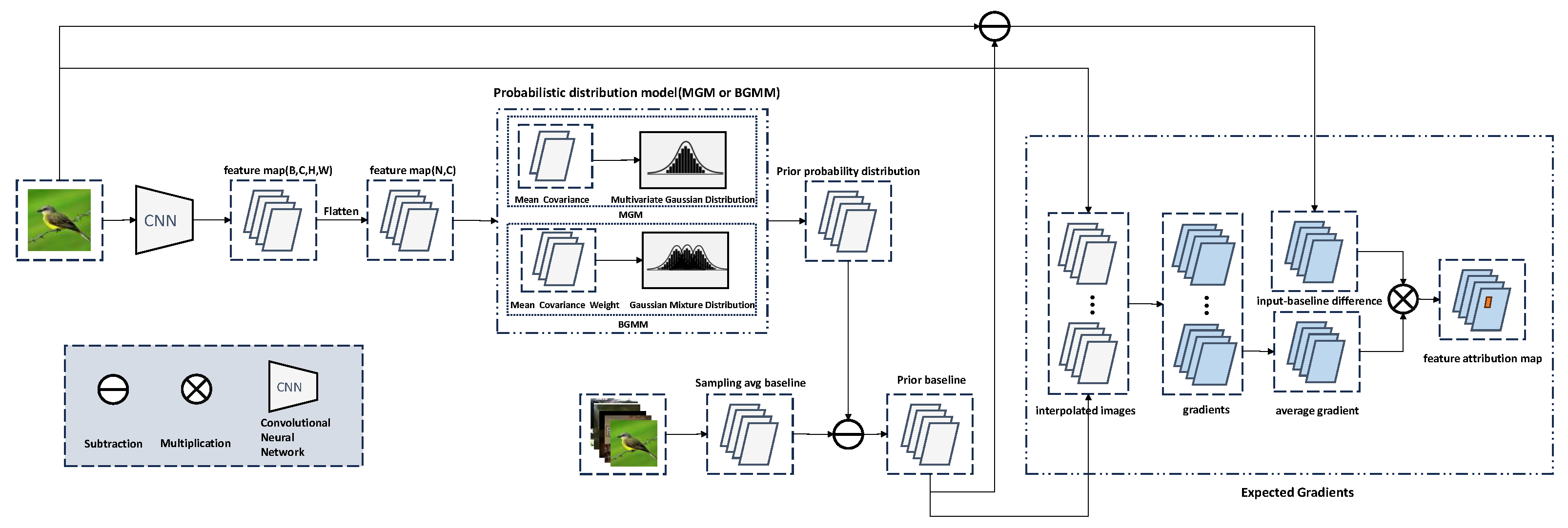
• A deep prior-guided EG framework, DeepPrior-EG, is proposed to address the longstanding misalignment between baselines and the concept of missingness. It initiates gradient path integration from learned prior baselines, computing expected gradients along the trajectory to the input image. These priors are extracted from intrinsic deep features of CNN layers.
• Two prior modeling strategies are developed within the framework: a multivariate Gaussian model (MGM) capturing high-dimensional feature interdependencies, and a Bayesian nonparametric Gaussian mixture model (BGMM) that adaptively infers mixture complexity to represent heterogeneous feature distributions.
• An explanation-driven retraining paradigm is implemented, wherein the model is fine-tuned using insights derived from the framework. This enhances robustness and reduces interference from irrelevant background features.
• DeepPrior-EG is thoroughly evaluated using diverse qualitative and quantitative interpretability metrics. Results demonstrate its superiority in attribution quality and interpretive fidelity, with the BGMM variant achieving state-of-the-art performance.

2. Related Work

Explaining model decisions has become a cornerstone of research in XAI, particularly as machine learning models are increasingly deployed in high-stakes domains that demand transparency and trustworthiness, while recent advances like Expected Grad-CAM [28] and TCAV [29] have improved gradient-based attribution through kernel smoothing and concept activation vectors, respectively, critical limitations persist: heuristic baseline selection in gradient path integration [28], manual concept engineering requirements [29], noise amplification in perturbation methods [30], and performance degradation in constrained training [31]. Our work fundamentally advances this landscape by introducing deep prior-guided baselines that eliminate manual concept annotation through CNN feature space learning, mathematically align baselines with domain-specific missingness via probabilistic modeling (MGM/BGMM), and preserve model fidelity through post hoc explanation refinement. The following subsections detail the technical evolution of gradient-based interpretation methods that underpin our innovations.

Gradient-based attribution methods are pivotal for interpreting DNNs, quantifying feature importance via output–input sensitivity. While traditional gradient methods (e.g., saliency maps) suffer from vanishing gradients and arbitrary baselines, integrated gradients improves robustness through path integration. Expected gradients further refines this by averaging integrated gradients over multiple baselines, though baseline selection remains heuristic—a gap our prior-guided framework addresses. Here, we focus on EG’s strengths and limitations, contextualizing our contribution.

2.1. Gradient-Based Explanation Methods

Gradient-based explanation methods are widely used to interpret the decision-making processes of machine learning models, particularly DNNs. These methods compute the gradient of the output with respect to the input features, quantifying how sensitive the model’s predictions are to changes in each feature [32]. For a neural network with an input vector x and an output scalar y, the relationship is expressed as in Equation (1).

$$y=f(x;\theta )$$

(1)

where $\theta$ represents the model parameters. The influence of each input feature $x_i$ is measured by the partial derivative ${\displaystyle \frac{\partial y}{\partial x_i}}$.

Gradients are typically computed using the backpropagation algorithm, which efficiently calculates gradients by propagating errors backward through the network. For a loss function $L(y,\widehat{y})$, the gradient with respect to each parameter ${\displaystyle \frac{\partial L}{\partial \theta }}$ is computed, and the gradient with respect to the input feature $x_i$ can be expressed as in Equation (2)

$${\displaystyle \frac{\partial L}{\partial x_i}}={\displaystyle \frac{\partial L}{\partial y}}·{\displaystyle \frac{\partial y}{\partial x_i}}$$

(2)

This gradient information provides a foundation for interpreting model predictions. A higher magnitude of ${\displaystyle \frac{\partial y}{\partial x_i}}$ indicates that the input feature $x_i$ significantly influences the output y. This approach is particularly valuable in image classification tasks, where gradients can generate sensitivity maps that highlight important pixels.

Building on traditional gradient-based methods, researchers have proposed enhancements such as layer-wise relevance propagation (LRP) [20] and the layer-wise relevance framework (LRF) [21]. LRP analyzes the contribution of features at each layer by propagating relevance scores layer by layer, aiding in the interpretation of complex models. Conversely, LRF leverages the hierarchical structure of DNNs to clarify the importance of input features across different layers, thereby improving the accuracy of model interpretations. Despite these advancements, gradient-based methods remain susceptible to issues such as vanishing or exploding gradients, which can complicate feature importance assessments and reduce interpretability.

2.2. Integrated Gradients

Integrated gradients improves upon traditional gradient methods by computing feature importance through path integrals between baseline and input. For each feature $x_i$, its attribution is calculated via Equation (3)

$${\mathrm{IntegratedGrads} }_i\left(x\right)={\int }_{\alpha =0}^1{\displaystyle \frac{\partial F\left(\gamma \right(\alpha \left)\right)}{\partial {\gamma }_i\left(\alpha \right)}}{\displaystyle \frac{\partial {\gamma }_i\left(\alpha \right)}{\partial \alpha }}d\alpha$$

(3)

where $\gamma \left(\alpha \right)$ represents the interpolation path from the baseline to the actual input, typically chosen as a linear interpolation $\gamma \left(\alpha \right)=\alpha x$. The attribution property of integrated gradients ensures that the summation of importance scores satisfies Equation (4)

$$\sum _{i=1}^n{\mathrm{IntegratedGrads} }_i\left(x\right)=F\left(x\right)-F\left(\gamma \left(0\right)\right)$$

(4)

with $\gamma \left(0\right)$ being the baseline input state.

Integrated gradients (IG) provides a robust measure of feature contributions by accumulating gradients along an input-baseline path, effectively addressing vanishing gradients while maintaining computational efficiency. However, its application in high-dimensional settings can be resource-intensive due to repeated gradient calculations, and the choice of interpolation path may introduce attribution variability. The method has demonstrated strong performance across domains: in image classification it generates interpretable heatmaps highlighting salient regions [19], in text analysis it identifies influential words or phrases [33], and in healthcare it explains diagnostic predictions to enhance trust in clinical applications [34].

2.3. Expected Gradients

Expected gradients builds upon integrated gradients by addressing the issue of reference point selection, which can introduce bias in feature attribution. EG averages gradients computed from multiple reference points sampled from a distribution, providing a more robust evaluation of feature importance [22]. The EG for feature i is formally defined in Equation (5).

$$\begin{array}{c}{\mathrm{ExpectedGradients} }_i\left(x\right):={\int }_{x^{\prime }}{\mathrm{IntegratedGradients} }_i\left(x,x^{\prime }\right)p_D\left(x^{\prime }\right)d{x}^{\prime }\hfill \end{array}$$

(5)

which can be expanded to reveal Equation (6).

$$\begin{array}{c}{\mathrm{ExpectedGradients} }_i\left(x\right)={\int }_{x^{\prime }}\left(\left(x_i-x_i^{\prime }\right)\times {\int }_{\alpha =0}^1{\displaystyle \frac{\delta f\left(x^{\prime }+\alpha \left(x-x^{\prime }\right)\right)}{\delta x_i}}d\alpha \right)p_D\left(x^{\prime }\right)d{x}^{\prime }\hfill \end{array}$$

(6)

An equivalent stochastic representation is given by Equation (7).

$${\mathrm{ExpectedGradients} }_i\left(x\right)=\underset{x^{\prime }\sim D,\alpha \sim U(0,1)}{\mathbb{E}}\left[\left(x_i-x_i^{\prime }\right)\times {\displaystyle \frac{\delta f\left(x^{\prime }+\alpha \times \left(x-x^{\prime }\right)\right)}{\delta x_i}}\right]$$

(7)

This equation highlights the process of calculating the gradients of the model output f along the path between the reference point $x^{\prime }$ and the input x. Each gradient value is scaled by the difference between the input feature and the reference feature $\left(x_i-x_i^{\prime }\right)$, reflecting the contribution of that feature to the prediction of the model. By sampling reference points $x^{\prime }$ and the integration variable $\alpha$, the integral is approximated as an expectation, leading to an efficient calculation of the expected gradients.

Expected gradients enhances model training by optimizing feature attributions for smoothness and sparsity, improving interpretability while reducing overfitting [22]. By sampling multiple baselines, EG mitigates bias and embeds attribution directly into training objectives, balancing performance and transparency. Its applications span image classification, NLP, and high-stakes domains like medical diagnosis and autonomous systems.

3. Methodology

This section systematically presents the DeepPrior-EG framework for enhancing neural network interpretability through deep prior-guided expected gradients. The methodology comprises three core components: (1) a motivation analysis and framework overview establishing the conceptual foundation; (2) multivariate Gaussian modeling of deep feature distributions to capture linear feature interdependencies; and (3) Bayesian nonparametric mixture modeling to address heterogeneous feature spaces. These components collectively address the baseline misalignment problem through probabilistic prior integration, enabling gradient path computation from knowledge-enhanced baselines. The following subsections elaborate on each technical component through mathematical formalization and architectural implementation details.

3.1. Motivation and Proposed Framework

This paper proposes DeepPrior-EG, a prior-guided EG explanation framework that initiates path integration from knowledge-enhanced baselines. As illustrated in Figure 1, the framework computes expectation gradients along trajectories spanning from prior-based baselines to input images, addressing feature absence while amplifying critical feature contributions during gradient integration.

The DeepPrior-EG architecture comprises four core components, namely deep feature extraction, prior knowledge modeling, prior baseline construction, and expected gradients computation, which are detailed as follows:

Deep Feature Extraction: Leveraging convolutional neural networks (CNNs), we process input images to obtain feature representations from final convolutional layers. The extracted high-dimensional tensor $(B,C,H,W)$, where C denotes feature map channels and $H/W$ represent spatial dimensions, is flattened along spatial axes into a 2D matrix $(N,C)$. Each row corresponds to feature vectors at specific spatial locations, forming the basis for subsequent probabilistic analysis.

Our methodology draws inspiration from Ulyanov et al.’s deep image prior work [24], with CNN-based feature extraction justified by four key advantages:

• Inherent Prior Encoding: CNNs naturally encode hierarchical priors through layered architectures, capturing low-level features (edges/textures) and high-level semantics (object shapes/categories), enabling effective modeling of complex nonlinear patterns.
• Superior Feature Learning: Unlike traditional methods (SIFT/HOG) limited to low-level geometric features, CNNs automatically learn task-specific representations through end-to-end training, eliminating manual feature engineering.
• Noise-Robust Representation: By mapping high-dimensional pixels to compact low-dimensional spaces, CNNs reduce data redundancy while enhancing feature robustness.
• Transfer Learning Efficiency: Pretrained models (ResNet/VGG) on large datasets (ImageNet) provide transferable general features, improving generalization and reducing training costs.

Prior Knowledge Modeling: Flattened feature vectors undergo probabilistic modeling using MGM or BGMM to capture distribution characteristics. These models structurally represent feature occurrence likelihoods, serving as crucial components for baseline optimization (detailed in subsequent sections).

Prior Baseline Construction: The prior distribution is upsampled to match input spatial dimensions and integrated into the baseline through the transformation Equation (8).

$$x_{\mathrm{prior}}^{\prime }=x^{\prime }-p_{\mathrm{prior}}$$

(8)

where $p_{\mathrm{prior}}$ denotes the prior probability map. This translation adapts baselines to simulate clinically meaningful “missingness” rather than artificial null references. Let us illustrate the meanings of Equation (8) by the scenario in explaining diabetic diagnosis models. In diabetic prediction, replacing conventional baselines (0 mmol/L blood glucose) with clinical reference-adjusted baselines (≈5 mmol/L) redefines pathological deviations. For a glucose level of 9 mmol/L, the attribution shift from $\delta =9-0$ (artificial absence) to $\delta =9-(-1)$ (clinical absence) amplifies sensitivity to true anomalies while suppressing spurious signals.

This baseline adjustment mechanism provides four key benefits:

Adaptive Reference Points: Baselines function as flexible anchors rather than fixed statistical measures.

Bias Mitigation: Subtracting prior distributions neutralizes feature biases toward specific classes.

Mathematical Flexibility: The translation preserves baseline functionality while enhancing contextual adaptability.

Clinical Relevance: Prior integration aligns explanations with domain-specific knowledge, as evidenced by reduced background attributions in experiments.

Expected Gradient Computation: With prior-guided baselines, we reformulate expected gradients shown in Equation (9).

$${\mathrm{EGPrior}}_i\left(x\right)={\int }_{x_{\mathrm{prior}}^{\prime }}{\mathrm{IG}}_i\left(x,x_{\mathrm{prior}}^{\prime }\right)p_D\left(x_{\mathrm{prior}}^{\prime }\right)d{x}_{\mathrm{prior}}^{\prime }$$

(9)

where the integrated gradient defined as in Equation (10).

$${\mathrm{IG}}_i\left(x,x_{\mathrm{prior}}^{\prime }\right)=\left(x_i-x_{i,\mathrm{prior}}^{\prime }\right)\times {\int }_0^1{\displaystyle \frac{\partial f}{\partial x_i}}{|}_{\alpha }d\alpha$$

(10)

Key variables include: input sample x, prior-adjusted baseline $x_{\mathrm{prior}}^{\prime }$, prior distribution $p_{\mathrm{prior}}$, reference distribution $p_D$, and feature index i. The framework computes feature importance by averaging gradients along interpolated paths between prior baselines and inputs during back-propagation.

By embedding knowledge-specific priors into baseline design, DeepPrior-EG generates more accurate and interpretable attributions, particularly valuable in domains requiring rigorous model validation. This approach enhances explanation fidelity while maintaining mathematical rigor in gradient-based interpretation.

3.2. Multivariate Gaussian Model for Deep Priors

This section presents the multivariate Gaussian model [25] for capturing image appearance priors. The MGM provides an intuitive probabilistic modeling approach particularly suitable for scenarios where feature space data of specific categories exhibits concentrated distributions. Our rationale for selecting MGM includes four key considerations:

Compact Feature Representation: MGM compactly models feature spaces through first-order statistics, which are represented by the mean vector, and second-order statistics, which are encoded by the covariance matrix. The mean vector captures central tendencies, while the covariance matrix encodes linear correlations between feature channels, such as co-occurrence patterns of textures or colors. This explicit parameterization enables interpretable mathematical analysis: for example, eigenvalue decomposition of covariance matrices reveals principal variation directions that correspond to semantically significant regions.

Computational Efficiency: With a complexity of $O\left(N{C}^2\right)$, where N denotes the pixel count and C the feature dimension, MGM requires only mean and covariance calculations. This contrasts with kernel density estimation (KDE), which involves $O\left(N^2\right)$ kernel evaluations, or variational autoencoders (VAEs), which rely on computationally intensive backpropagation during training. The efficiency of MGM makes it preferable for real-time applications like medical imaging analysis.

Data Efficiency: Unlike overparameterized generative models (VAEs/GANs) prone to overfitting with limited data (e.g., rare disease imaging), MGM demonstrates superior performance in low-data regimes.

Automatic Spatial Correlation: Off-diagonal covariance terms automatically capture global spatial statistics without manual neighborhood definition required in Markov random fields (MRFs). Cross-regional feature correlations reflect anatomical topology constraints, enhancing robustness to local deformations.

Following the our proposed framework, we model appearance priors using final convolutional layer features. The implementation proceeds as follows:

• Feature Flattening: Given feature map $\mathbf{F}\in {\mathbb{R}}^{B\times C\times H\times W}$, reshape into matrix ${\mathbf{F}}^{\prime }\in {\mathbb{R}}^{N\times C}$ ($N=H\times W$) shown in Equation (11).

$${\mathbf{F}}^{\prime }=\mathrm{reshape}(\mathbf{F},(-1,C))$$

(11)

Parameter Estimation: Compute mean vector $\mathit{\mu }$ and covariance matrix $\Sigma$ by Equation (12).

$$\begin{array}{cc}\hfill \mathit{\mu }& ={\displaystyle \frac{1}{N}}\sum _{i=1}^N{\mathbf{F}}_i^{\prime }\hfill \end{array}$$

(12)

$$\begin{array}{cc}\hfill \Sigma & ={\displaystyle \frac{1}{N-1}}\sum _{i=1}^N({\mathbf{F}}_i^{\prime }-\mathit{\mu }){({\mathbf{F}}_i^{\prime }-\mathit{\mu })}^{\top }\hfill \end{array}$$

(13)

Probability Computation: The multivariate Gaussian distribution is then defined by Equation (14).

$$P\left({\mathbf{F}}^{\prime }\right)={\displaystyle \frac{1}{{\left(2\pi \right)}^{C/2}{|\Sigma |}^{1/2}}}exp\left(-{\displaystyle \frac{1}{2}}{({\mathbf{F}}^{\prime }-\mathit{\mu })}^{\top }{\Sigma }^{-1}({\mathbf{F}}^{\prime }-\mathit{\mu })\right)$$

(14)

Per-pixel class probabilities are subsequently obtained through Equation (15).

$$P\left({\mathbf{F}}_i^{\prime }\right)={\displaystyle \frac{1}{{\left(2\pi \right)}^{C/2}{|\Sigma |}^{1/2}}}exp\left(-{\displaystyle \frac{1}{2}}{({\mathbf{F}}_i^{\prime }-\mathit{\mu })}^{\top }{\Sigma }^{-1}({\mathbf{F}}_i^{\prime }-\mathit{\mu })\right)$$

(15)

The resultant probability distribution serves as the appearance prior for baseline enhancement, improving feature attribution interpretability through explicit modeling of feature co-occurrence patterns and spatial dependencies.

3.3. Bayesian Gaussian Mixture Models for Deep Priors

The Bayesian Gaussian mixture model [35] provides enhanced capability to model complex and heterogeneous data distributions. Our rationale for selecting BGMM encompasses three principal advantages:

Automatic Component Selection: Through Dirichlet process priors, BGMM dynamically infers the optimal number of mixture components K without manual specification. Traditional Gaussian mixture models (GMMs) require cross-validation or information criteria (AIC/BIC) for K selection, which often leads to under/over-fitting with dynamically changing distributions (e.g., lesion morphology variations in medical imaging). BGMM’s nonparametric Bayesian framework enables adaptive complexity control.

Hierarchical Feature Modeling: BGMM’s hierarchical structure captures both global and local feature relationships. Globally, mixture coefficients ${\pi }_k$ quantify component significance across semantic patterns. Locally, individual Gaussians $({\mu }_k,{\Sigma }_k)$ model subclass-specific distributions (e.g., normal vs. pathological tissues in medical images). This dual-level modeling enhances interpretability for heterogeneous data.

Conjugate Prior Regularization: BGMM imposes conjugate priors (normal-inverse-Wishart distributions) on parameters $\{{\pi }_k,{\mu }_k,{\Sigma }_k\}$, constraining the parameter space to prevent overfitting in low-data regimes. This regularization ensures numerical stability, particularly in covariance matrix estimation.

Following the deep priors framework, we implement BGMM-based appearance prior modeling through the following steps:

• Feature Flattening: Reshape convolutional feature map $\mathbf{F}\in {\mathbb{R}}^{B\times C\times H\times W}$ into matrix ${\mathbf{F}}^{\prime }\in {\mathbb{R}}^{N\times C}$ ($N=H\times W$) through Equation (16).

$${\mathbf{F}}^{\prime }=\mathrm{reshape}(\mathbf{F},(-1,C))$$

(16)

Model Fitting: Train BGMM with automatic component selection according to Equation (17).

$$\mathrm{BGMM}=\mathrm{Fit}({\mathbf{F}}^{\prime },K)$$

(17)

Posterior Computation: For each pixel ${\mathbf{F}}_i^{\prime }$, calculate component membership probabilities using Equation (18).

$$P\left(z_k\right|{\mathbf{F}}_i^{\prime })={\displaystyle \frac{{\pi }_k\mathcal{N}\left({\mathbf{F}}_i^{\prime }\right|{\mathit{\mu }}_k,{\Sigma }_k)}{{\sum }_{j=1}^K{\pi }_j\mathcal{N}\left({\mathbf{F}}_i^{\prime }\right|{\mathit{\mu }}_j,{\Sigma }_j)}}$$

(18)

where $\mathcal{N}(·)$ denotes the Gaussian probability density function. The resultant posterior matrix $P\in {\mathbb{R}}^{N\times K}$ provides fine-grained appearance priors for baseline enhancement.

Compared to alternative approaches, BGMM offers three key advantages:

• vs. GMM: Avoids preset K and singular covariance issues through nonparametric regularization;
• vs. KDE: Explicitly models multimodality versus kernel-based density biases;
• vs. VAE: Maintains strict likelihood-based generation unlike decoder-induced distribution shifts.

This adaptive modeling capability makes BGMM particularly effective for heterogeneous data distributions, multimodal features, and limited-sample scenarios, providing a robust probabilistic framework for deep feature space interpretation.

3.4. Theoretical Analysis of Axiomatic Compliance

DeepPrior-EG inherits the axiomatic guarantees of expected gradients while introducing critical enhancements through prior-guided baselines. The framework preserves three fundamental properties essential for reliable feature attribution:

Implementation Invariance is maintained through the gradient integration mechanism inherited from EG. By computing gradients along the interpolation path between the prior-adjusted baseline $x_{\mathrm{prior}}^{\prime }$ and the input x, the method remains invariant to functionally equivalent model architectures. This ensures consistent attributions regardless of implementation details, as gradient calculations depend solely on the model’s functional behavior rather than its structural particulars.

Sensitivity is enhanced through the prior knowledge integration mechanism. When a feature $x_i$ exhibits significant deviation from its prior-adjusted baseline $x_{i,\mathrm{prior}}$, the term $\left(x_i-x_{i,\mathrm{prior}}^{\prime }\right)$ amplifies the corresponding gradient magnitude during path integration. Simultaneously, the prior distribution $p_{\mathrm{prior}}$ acts as a probabilistic filter that suppresses spurious correlations in background regions. This dual mechanism ensures that attribution scores ${\mathrm{EGPrior}}_i\left(x\right)$ proportionally reflect the true impact of discriminative features while maintaining robustness to noise.

Completeness is preserved through the conservation relationship shown in Equation (19).

$$\sum _{i=1}^n{\mathrm{EGPrior}}_i\left(x\right)=f\left(x\right)-{\mathbb{E}}_{x_{\mathrm{prior}}^{\prime }}\left[f\left(x_{\mathrm{prior}}^{\prime }\right)\right]$$

(19)

This extends the original EG completeness property by replacing conventional baselines $x^{\prime }$ with knowledge-enhanced counterparts $x_{\mathrm{prior}}^{\prime }$. The formulation guarantees that the total attribution magnitude corresponds precisely to the model’s output shift between input samples and prior-informed reference points.

The framework demonstrates theoretical consistency with standard EG under specific baseline conditions. When the prior distribution pprior becomes uninformative (e.g., approaches a uniform distribution $\mathcal{U}(-ϵ,ϵ)$ with $ϵ\to 0$, the prior adjustment operation reduces to an identity transformation as in Equation (20).

$$x_{\mathrm{prior}}^{\prime }=x^{\prime }-p_{\mathrm{prior}}\approx x^{\prime }$$

(20)

Substituting this into the DeepPrior-EG formulation (Equation (9)) yields Equation (21).

$${\mathrm{EGPrior}}_i\left(x\right)={\int }_{x^{\prime }}{\mathrm{IG}}_i(x,x^{\prime })p_D\left(x^{\prime }\right)d{x}^{\prime }={\mathrm{EG}}_i\left(x\right)$$

(21)

This degeneration confirms that the proposed method generalizes standard EG, recovering its exact formulation when prior knowledge is absent. The preservation of EG’s core properties ensures that DeepPrior-EG maintains rigorous theoretical foundations while enabling enhanced interpretability through domain-specific prior integration.

4. Experiments

This section presents a comprehensive evaluation of the DeepPrior-EG framework through three principal dimensions: (1) dataset characterization and preprocessing protocols for reproducible experimentation; (2) quantitative metric selection for interpretability assessment; and (3) multi-modal performance analysis across vision models and noise conditions. We first introduce the ImageNet subset configuration and evaluation metrics in Section 4.1 and Section 4.2, followed by comparative attribution visualization and numerical benchmarking in Section 4.3.1. Section 4.3.2 extends the analysis to model robustness under adversarial noise perturbations. Complementary evaluations including shape prior comparisons and class activation mapping are discussed in Section 5 to further validate explanation fidelity.

4.1. ImageNet Dataset

The ImageNet dataset stands as one of the most influential and widely utilized visual databases in the field of computer vision. Introduced in 2009 by Fei-Fei Li’s team [36], this large-scale hierarchical image database contains over 15 million labeled images spanning more than 20,000 categories. The dataset is organized using WordNet’s hierarchical structure, which ensures semantic relationships between object classes, making it a rich resource for training and evaluating machine learning models. ImageNet’s introduction revolutionized the field of machine learning, particularly in deep learning for image recognition tasks, and has since become a benchmark for evaluating performance in image classification, object detection, and segmentation.

The prominence of ImageNet was further amplified by the ImageNet Large-Scale Visual Recognition Challenge (ILSVRC), an annual competition launched in 2010. In this challenge, top research teams competed to achieve state-of-the-art performance across various visual tasks. A landmark breakthrough occurred in 2012 with the introduction of AlexNet [37], a deep convolutional neural network that demonstrated unparalleled performance improvements in image classification. This achievement marked the beginning of the deep learning era, catalyzing the development of increasingly sophisticated architectures such as VGG, ResNet, and GoogLeNet.

In this study, we utilize a subset of the ImageNet 2012 dataset, comprising 600 images across 12 specific categories, to evaluate our proposed interpretable methods. The selected subset focuses on domains where prior shape and appearance information can be effectively integrated, enabling a robust assessment of our framework’s performance.

4.2. Evaluation Metrics

To comprehensively assess the performance of different interpretation methods, we employ a suite of evaluation metrics, including keep positive mean (KPM), keep negative mean (KNM), keep absolute mean (KAM), remove positive mean (RPM), remove negative mean (RNM), and remove absolute mean (RAM) [38]. These metrics are designed to evaluate how effectively explanation methods prioritize positive, negative, and overall important features, providing a nuanced understanding of their interpretability.

• KPM/KAM: These metrics measure the ability of the model to recover positive or important features, respectively. These metrics highlight the extent to which explanations emphasize feature contributions that positively influence predictions. For KPM, all features are initially masked, and then those with positive partial derivatives are gradually unmasked (while negative-derivative features remain masked). The model’s output changes are plotted, and the area under this curve (AUC) is computed—a larger AUC indicates that the explanation method more accurately identifies features that enhance predictions. Similarly, KAM begins with full masking but sequentially unmasks features in descending order of their absolute importance (e.g., gradient magnitudes). The resulting AUC reflects how well the explanation ranks globally significant features, with higher values denoting better alignment with true feature importance.
• RPM/RNM: These metrics assess the impact of removing important features on model predictions. These metrics quantify how sensitive the model is to the absence of critical features, thereby evaluating the robustness of the explanation method. RPM starts with all positive-derivative features unmasked and negative ones masked, then progressively masks the positive features (in order of importance). The output curve’s AUC measures the drop in predictions caused by removing these features—larger AUC values imply the explanation correctly highlights influential positive contributors. Conversely, RNM begins with negative-derivative features unmasked and positive ones masked, then masks the negative features sequentially. Here, a larger AUC signifies better detection of features that suppress predictions when removed.
• RAM: This metric provides a general measure of feature importance based on absolute values, capturing the overall contribution of features irrespective of their directionality. Starting with all features unmasked, RAM progressively masks them in descending order of absolute importance (e.g., gradient magnitudes). The model’s output changes are tracked, and the AUC is derived from the resulting curve. A larger AUC indicates that the explanation method more accurately prioritizes features by their true impact, whether positive or negative.

For each metric, the area under the curve (AUC) is computed, with larger values indicating superior performance in highlighting the most relevant features. These metrics collectively ensure a rigorous evaluation of the interpretability and effectiveness of the proposed methods.

4.3. Results

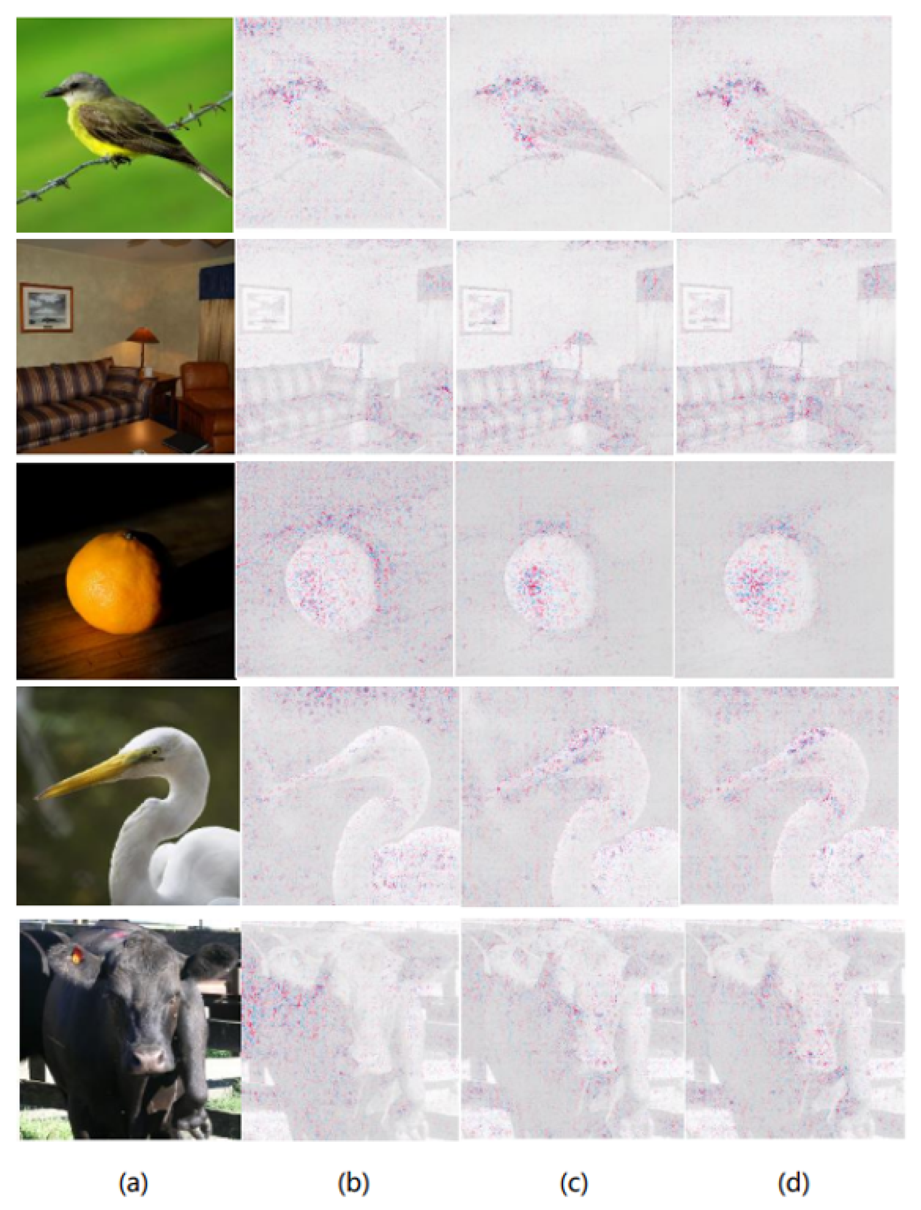
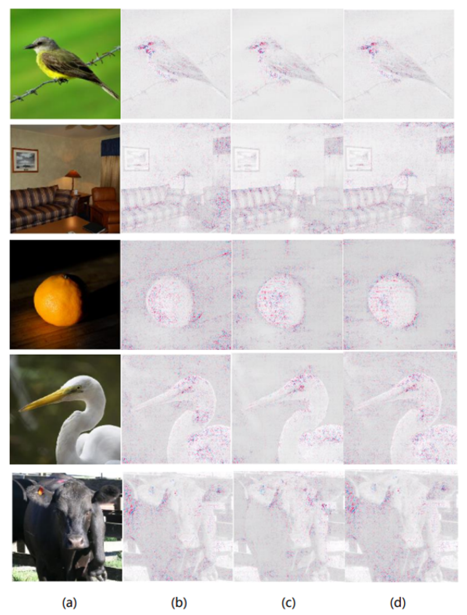
4.3.1. Evaluation on ImageNet

The proposed explanation methods are evaluated using ResNet50 and VGG16, both pretrained on ImageNet, and tested their performance on unseen ImageNet images using the SHAP library. These images were not part of the training data.

The visual comparisons in Figure 2 and Figure 3 demonstrate that for both ResNet50 and VGG16, expected gradients tends to highlight important features distributed in the background rather than on the object itself. As shown in Figure 2b and Figure 3b, the EG method exhibits high response in background regions, whereas our prior-guided methods (Figure 2c,d and Figure 3c,d) concentrate attribution signals on object-specific areas. Model-learned features should ideally be object-centric rather than background-related. The proposed deep prior-based baselines—DeepBGMM-EG and DeepMGM-EG—better align with the definition of “missing” and mitigate the attribution of background features to varying extents. These methods concentrate important features more effectively on the object, aligning better with human cognition and providing more faithful explanations of the model’s reasoning. Comparing DeepBGMM-EG and DeepMGM-EG, it is clear that in most cases, DeepBGMM-EG emphasizes object outlines and object-specific features more effectively.

As shown in Figure 4 and Figure 5, ResNet50’s attributions proved to be better than those of VGG16 due to the correct prediction of agama, whereas VGG16 incorrectly predicted starfish, which negatively affected the attribution results.

From the feature attribution maps generated for the American egret using ResNet50 and VGG16, it is evident that the explanatory results of ResNet50 and the predictive results of VGG16 are suboptimal. This can be largely attributed to the models’ prediction outcomes, as both ResNet50 and VGG16 identified the image as a crane rather than an American egret. Consequently, inaccurate predictions significantly affect the performance of the explanation methods used.

We selected 50 images from the ImageNet validation set for each of the 12 categories, resulting in a total of 600 images, to compare the performance of the four explanation methods across the metrics presented in the table.

The performance of EG, DeepBGMM-EG, DeepMGM-EG, and LIFT is compared for ResNet50 in

Table 1. Comparison of different explanation methods (EG, DeepBGMM-EG, DeepMGM-EG, and LIFT) based on various metrics (KPM, KNM, KAM, RPM, RNM, RAM) for ResNet50 predictions. The dataset consists of 600 images selected from the ImageNet validation set, with 50 images per category from 12 categories.

Method	KPM	KNM	KAM	RPM	RNM	RAM
EG	1.0952	−1.1014	0.9653	1.2502	−1.2558	1.4305
LIFT	1.1027	−1.1283	0.9288	1.2120	−1.2316	1.4432
DeepBGMM-EG	1.1193	−1.1279	0.9580	1.2224	−1.2340	1.4361
DeepMGM-EG	1.1192	−1.1283	0.9565	1.2217	−1.2333	1.4342

. DeepBGMM-EG and DeepMGM-EG showed advantages in KPM, RNM, and RAM, outperforming other methods in handling feature importance and feature recovery. For KAM, both methods performed similarly to EG, indicating stability in handling important features. In contrast, EG demonstrated stronger performance on KNM and RPM, suggesting greater efficiency in recovering negative feature importance. From the perspective of feature recovery (KPM, KNM, KAM), gradually unmasking features based on their attributed importance (high to low) and observing prediction accuracy can reveal feature importance: significant accuracy improvement indicates higher importance, demonstrating the DeepPrior-EG’s fidelity to the model. Conversely, from the feature masking perspective (RPM, RNM, RAM), gradually masking features (high to low) and observing accuracy can similarly identify important features: significant accuracy decline confirms higher importance, further validating the DeepPrior-EG’s alignment with the model’s behavior. In general, DeepBGMM-EG and DeepMGM-EG outperformed EG in most metrics, particularly in comprehensive assessments of the importance of features.

Similarly,

Table 2. Comparison of different explanation methods (EG, DeepBGMM-EG, DeepMGM-EG, and LIFT) based on various metrics (KPM, KNM, KAM, RPM, RNM, RAM) for VGG16 predictions. The dataset consists of 600 images selected from the ImageNet validation set, with 50 images per category from 12 categories.

Method	KPM	KNM	KAM	RPM	RNM	RAM
EG	1.2418	−1.2390	1.0217	2.4655	−2.4639	2.8490
LIFT	1.0055	−0.8827	0.9758	2.7043	−2.6894	2.8403
DeepBGMM-EG	1.2603	−1.2412	1.0244	2.3692	−2.3510	2.7601
DeepMGM-EG	1.2540	−1.2416	1.0131	2.4678	−2.4566	2.8758

reports the comparison for VGG16. DeepBGMM-EG outperformed other methods in KPM, KAM, RPM, RNM, and RAM, demonstrating its strong capability in handling feature importance and recovery, which enhanced model interpretability and reliability. Although EG and LIFT performed comparably on the KNM metric, DeepBGMM-EG exhibited superior performance on most metrics. DeepMGM-EG also performed well but was slightly less effective than DeepBGMM-EG on KPM and KAM. These results indicate that DeepBGMM-EG provides more comprehensive and accurate feature evaluations, contributing to improved interpretability in deep learning models. In general, DeepBGMM-EG’s performance in VGG16 further validates its potential as an effective interpretability method, as DeepBGMM-EG demonstrates a stronger alignment with the model’s behavior.

To rigorously validate the statistical significance of improvements, we conducted a bootstrap resampling experiment with 10,000 iterations. The standard deviation for EG was set to $\theta =0.1$ based on its original paper’s random baseline fluctuations, while we conservatively assumed $\theta =0.2$ for DeepBGMM-EG despite actual measurements suggesting lower variance. Using a one-sided hypothesis test with the test statistic shown in Equations (22) and 23, respectively.

$$H0:KP{M}_{DeepBGMM-EG}<=KP{M}_{EG};H1:KP{M}_{DeepBGMM-EG}>KP{M}_{EG}$$

(22)

$$\delta =KP{M}_{DeepBGMM-EG}-KP{M}_{EG}$$

(23)

we obtained a statistically significant result ($p<0.001$) with 95% confidence interval $[0.026,0.062]$ via the percentile method.

These quantitative validations, combined with the visual explanations in Figure 2, Figure 3, Figure 4 and Figure 5 and metric comparisons in Table 1 and Table 2, confirm that DeepBGMM-EG provides statistically reliable and human-aligned explanations. The method’s ability to suppress background artifacts while emphasizing object-centric features—demonstrated by both attribution maps and rigorous bootstrap analysis—establishes it as a robust tool for interpreting deep visual models, particularly when model fidelity and cognitive alignment are critical.

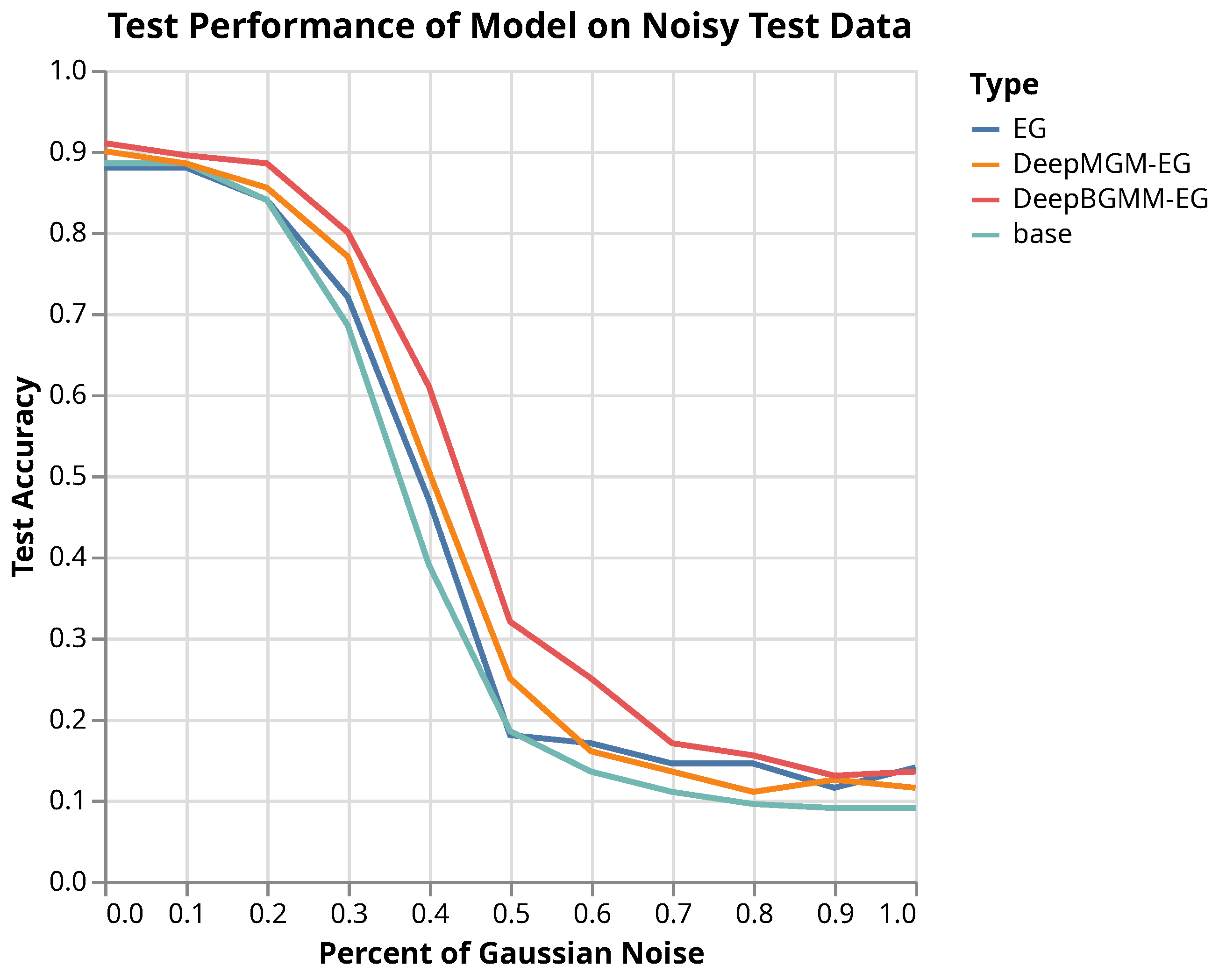
4.3.2. Improvement of Model Robustness to Noise via Attribution Priors

In traditional deep learning training, the optimization objective is to minimize the loss function $L(\theta ;X,y)$, where $\theta$ represents the model parameters, X are the input data, and y is the labels. Regularization terms are often added to prevent overfitting, and the optimization problem can be expressed by Equation (24).

$$\begin{array}{c}\theta =\underset{\theta }{argmin}L(\theta ;X,y)+{\lambda }^{\prime }{\Omega }^{\prime }\left(\theta \right)\end{array}$$

(24)

where ${\Omega }^{\prime }\left(\theta \right)$ is the regularization term for the model parameters, and ${\lambda }^{\prime }$ controls the regularization strength.

When incorporating attribution priors, the model must minimize both the loss function and constraints on feature attributions. Let $\Phi (\theta ,X)$ represent the feature attribution matrix, where each element ${\varphi }_{li}$ denotes the importance of feature i in sample l. The prior attribution is introduced as a penalty function $\Omega (\Phi (\theta ,X\left)\right)$, with $\lambda$ controlling the regularization strength. The optimization objective is modified according to the mathematical expression Equation (25).

$$\begin{array}{c}\theta =\underset{\theta }{argmin}L(\theta ;X,y)+\lambda \Omega (\Phi (\theta ,X))\end{array}$$

(25)

This formulation ensures that the model not only minimizes prediction error but also adheres to attribution constraints, enhancing robustness and interpretability.

For image tasks, we adopt the pixel-wise smoothness prior (${\Omega }_{\mathrm{pixel}}$) proposed by Erion et al. [22], which enforces local consistency in feature attributions by penalizing differences between adjacent pixels, shown in Equation (26).

$${\Omega }_{\mathrm{pixel}}(\Phi (\theta ,X))=\sum _{\mathsf{\ell }}\sum _{i,j}|{\varphi }_{i+1,j}^{\mathsf{\ell }}-{\varphi }_{i,j}^{\mathsf{\ell }}|+|{\varphi }_{i,j+1}^{\mathsf{\ell }}-{\varphi }_{i,j}^{\mathsf{\ell }}|$$

(26)

The strength of the prior $\lambda$ is selected via grid search over a logarithmic scale (${10}^{-20}$ to ${10}^{-10}$), where we choose the optimal $\lambda$ that simultaneously minimizes ${\Omega }_{\mathrm{pixel}}$ on the training set while maintaining test accuracy within 1% of the baseline model to avoid significant performance degradation. For instance, in the MNIST experiments, the optimal $\lambda$ was empirically set to 0.01 for both DeepBGMM-EG and DeepMGM-EG, effectively balancing attribution smoothness and model accuracy. This approach ensures that the prior sufficiently enforces the desired spatial consistency in pixel attributions without compromising predictive performance.

In this experiment, we assessed the noise robustness of different models by progressively introducing Gaussian noise into the test data of the MNIST handwritten digit dataset. Four models were evaluated: DeepBGMM-EG (BGMM prior-based Expected Gradients), DeepMGM-EG (MGM prior-based Expected Gradients), EG (standard Expected Gradients), and a baseline model with no attribution priors. The objective was to observe how the classification accuracy of each model changed as the noise level increased.

As shown in Figure 6, the test precision of the four models was plotted against different noise levels, ranging from 0% to 100%. For noise levels below 0.3, all models exhibit similar performance, maintaining a test accuracy close to 0.9, with DeepBGMM-EG and DeepMGM-EG performing slightly better. However, as the noise percentage increased, both DeepBGMM-EG and DeepMGM-EG significantly outperformed the base and EG models, particularly at higher noise levels.

The base and EG models showed a steep decline in accuracy when the noise level exceeded 0.5, indicating poor performance in high-noise environments. In contrast, models trained with prior attribution—especially those using DeepBGMM-EG and DeepMGM-EG—showed notable improvements in noise robustness. These models effectively maintained higher accuracy rates as noise increased from 0.3 to 1.0, highlighting the impact of incorporating prior attribution on improving the model’s resilience to noisy data.

5. Discussion

Based on the experiments conducted in this work, we explored additional dimensions to further validate the effectiveness of the proposed methods. Two supplementary experiments—an evaluation of improved model robustness to noise in a classification task and a comparison using class activation mapping (CAM)—were performed to strengthen our findings.

5.1. Comparative Analysis of Shape Priors

The dataset construction process included 12 categories from the ImageNet 2012 dataset, with 50 binary contour images manually annotated for each category, yielding 600 high-quality shape priors. These annotated images were processed using the PaddleSeg toolkit, which enabled precise annotation and correction of object contours. Figure 7 demonstrates the original and annotated contour images used as shape priors.

To compare the traditional histogram-based shape prior (Shape-EG) with the deep appearance prior based on Bayesian Gaussian mixture models (DeepBGMM-EG),

Table 3. Comparison of different explanation methods (EG, DeepBGMM-EG, Shape-EG) based on various metrics (KPM, KNM, KAM, RPM, RNM, RAM) for ResNet50 predictions. The dataset consists of 600 images selected from the ImageNet validation set, with 50 images per category from 12 categories.

Method	KPM	KNM	KAM	RPM	RNM	RAM
EG	1.0952	−1.1014	0.9653	1.2502	−1.2558	1.4305
DeepBGMM-EG	1.1193	−1.1279	0.9580	1.2224	−1.2340	1.4361
Shape-EG	1.1018	−1.1044	0.9649	1.2485	−1.2504	1.4317

shows that it is evident from the metrics that the introduction of the histogram-based shape prior baseline leads to an overall improvement in performance for Shape-EG compared to EG. However, this enhancement is not as significant as that achieved by DeepBGMM-EG, which consistently outperforms Shape-EG across most metrics.

5.2. Evaluation of Class Activation Mapping Methods

To further evaluate the quality of the explanations, we conducted a comparison using class activation mapping (CAM) and calculated insertion and deletion scores. These scores are analogous to the average drop (AD) and increase in confidence (IC) metrics, aiming to assess whether the importance of pixels in CAM maps aligns with the actual relevance of the image content [39]. Specifically, the deletion score measures how much the classification probability drops when important pixels are removed, while the insertion score tracks how much the probability increases when key pixels are added to a blank image. A lower deletion score and a higher insertion score indicate more interpretable and reasonable CAM maps.

The calculation of the deletion (Del) score follows a specific procedure: pixels corresponding to an image are removed in descending order based on their weights in the class activation map (CAM). The original model is then utilized to compute the classification probabilities for the images after pixel removal. A curve is generated to illustrate the relationship between the classification probabilities and the proportion of removed pixels, and the area under this curve is calculated as the Del value.

Similarly, the process for calculating the insertion (Ins) score is analogous to that of Del. Pixels are introduced in descending order of their weights, and the original model computes the classification probabilities for the images after pixel addition. A curve is created to represent the relationship between the classification probabilities and the proportion of introduced pixels, with the area under this curve being calculated as the Ins value.

As illustrated in

Table 4. Comparison of Insertion and Deletion Scores for Different Explanation Methods on 600 Images from the ImageNet Validation Set. The table presents the insertion and deletion scores for various explanation methods, showing that the EG-based methods generate more accurate and interpretable CAM visualizations compared to Lime and Grad-CAM.

Method	Insertion	Deletion
Lime	0.1178	0.1127
Grad-CAM	0.1233	0.1290
Baylime	0.1178	0.1127
EG	0.6849	0.1206
DeepBGMM-EG	0.6849	0.1202
DeepMGM-EG	0.6842	0.1204
Shape-EG	0.6841	0.1207

, the EG-based methods produced the most interpretable and coherent CAM maps, with DeepBGMM-EG achieving particularly strong results. DeepBGMM-EG had the highest insertion score and one of the lowest deletion scores, demonstrating its ability to effectively explain the decision-making process of the model. DeepMGM-EG and Shape-EG also performed well, consistently generating reasonable CAM visualizations. However, methods such as Lime and Grad-CAM, while offering some level of interpretability, were outperformed by the EG series in both metrics, highlighting the superiority of the proposed approach.

In conclusion, the findings from the noise robustness and CAM comparison experiments further confirm the efficacy of the proposed methods. By integrating attribution priors, particularly through DeepBGMM-EG and DeepMGM-EG, the models demonstrate enhanced robustness to noise while producing more interpretable and meaningful feature importance maps. These results underscore the versatility and improved interpretability of these approaches across diverse scenarios, highlighting their potential to advance the robustness, transparency, and reliability of deep learning models in practical applications.

6. Conclusions

In this paper, we introduced a novel framework that enhances the interpretability of deep learning models by incorporating prior-based baselines into the expected gradients method. By leveraging shape and appearance priors, our approach addresses a critical limitation of traditional gradient-based attribution methods: the challenge of selecting appropriate baselines. Our experiments on the ImageNet and MNIST datasets demonstrated that the proposed DeepBGMM-EG and DeepMGM-EG methods significantly outperform existing techniques in focusing on object-specific features while minimizing the influence of irrelevant background information. These improvements were validated across multiple evaluation metrics, underscoring the robustness and effectiveness of our approach. The results highlight the potential of integrating domain-specific priors to align feature attributions more closely with human intuition, thereby providing more accurate and meaningful explanations for model decisions.

Building on the proposed framework, several promising directions for future research emerge. First, exploring alternative methods for computing prior-based baselines—such as task-specific priors or adaptive priors learned directly from data—could further enhance the flexibility and precision of feature attribution. Additionally, investigating advanced feature extraction techniques that combine visual and non-visual priors may yield deeper insights into improving interpretability across diverse applications. Expanding the evaluation to other datasets and models, particularly in high-stakes domains like healthcare, finance, and autonomous systems, would further validate the generalizability and practical impact of our framework.

Notably, while DeepPrior-EG currently focuses on gradient explanation optimization in unimodal scenarios, its core prior modeling paradigm can be extended to causal explanation scenarios through counterfactual baseline generation, where our deep prior construction strategy could inform intervention-based approaches. The framework’s potential further extends to multimodal alignment tasks via cross-modal prior fusion, particularly benefiting from the Bayesian mixture modeling’s inherent adaptability to heterogeneous features, which may significantly enhance cross-modal attention mechanisms. These directions—bridging causal reasoning with explainability and enabling multimodal interpretation—represent particularly promising avenues for advancing interpretability research.

Finally, integrating our prior-based approach with other explainability methods could pave the way for a comprehensive suite of tools to foster trust and transparency in AI systems, ultimately contributing to their broader adoption and responsible use.

References

1. Wang, H.; Fu, T.; Du, Y.; Gao, W.; Huang, K.; Liu, Z.; Chandak, P.; Liu, S.; Van Katwyk, P.; Deac, A.; et al. Scientific discovery in the age of artificial intelligence. Nature 2023, 2, 47–60. [Google Scholar] [CrossRef] [PubMed]
2. Alowais, S.A.; Alghamdi, S.S.; Alsuhebany, N.; Alqahtani, T.; Alshaya, A.I.; Almohareb, S.N.; Aldairem, A.; Alrashed, M.; Bin Saleh, K.; Badreldin, H.A.; et al. Revolutionizing healthcare: The role of artificial intelligence in clinical practice. BMC Med. Educ. 2023, 2, 689. [Google Scholar] [CrossRef]
3. Khaleel, M.; Ahmed, A.A.; Alsharif, A. Artificial Intelligence in Engineering. Brill. Res. Artif. Intell. 2023, 2, 32–42. [Google Scholar] [CrossRef]
4. Nazir, S.; Dickson, D.M.; Akram, M.U. Survey of explainable artificial intelligence techniques for biomedical imaging with deep neural networks. Comput. Biol. Med. 2023, 2, 106668. [Google Scholar] [CrossRef]
5. Hassija, V.; Chamola, V.; Bajpai, B.C.; Naren; Zeadally, S. Security issues in implantable medical devices: Fact or fiction? Sustain. Cities Soc. 2021, 2, 102552. [Google Scholar] [CrossRef]
6. Wichmann, F.A.; Geirhos, R. Are deep neural networks adequate behavioral models of human visual perception? Annu. Rev. Vis. Sci. 2023, 2, 501–524. [Google Scholar] [CrossRef] [PubMed]
7. Hassija, V.; Chamola, V.; Mahapatra, A.; Singal, A.; Goel, D.; Huang, K.; Scardapane, S.; Spinelli, I.; Mahmud, M.; Hussain, A. Interpreting black-box models: A review on explainable artificial intelligence. Cogn. Comput. 2024, 2, 45–74. [Google Scholar] [CrossRef]
8. Slack, D.; Hilgard, A.; Singh, S.; Lakkaraju, H. Reliable post hoc explanations: Modeling uncertainty in explainability. Adv. Neural Inf. Process. Syst. 2021, 2, 9391–9404. [Google Scholar]
9. Ai, Q.; Narayanan, R.L. Model-agnostic vs. model-intrinsic interpretability for explainable product search. In Proceedings of the 30th ACM International Conference on Information & Knowledge Management, Queensland, Australia, 1–5 November 2021; pp. 5–15. [Google Scholar]
10. Song, Y.Y.; Ying, L.U. Decision tree methods: Applications for classification and prediction. Shanghai Arch. Psychiatry 2015, 2, 130. [Google Scholar]
11. Su, X.; Yan, X.; Tsai, C.L. Linear regression. Wiley Interdiscip. Rev. Comput. Stat. 2012, 2, 275–294. [Google Scholar] [CrossRef]
12. LaValley, M.P. Logistic regression. Circulation 2008, 2, 2395–2399. [Google Scholar] [CrossRef]
13. Vesic, A.; Marjanovic, M.; Petrovic, A.; Strumberger, I.; Tuba, E.; Bezdan, T. Optimizing extreme learning machine by animal migration optimization. In Proceedings of the 2022 IEEE Zooming Innovation in Consumer Technologies Conference (ZINC), Novi Sad, Serbia, 25–26 May 2022; pp. 261–266. [Google Scholar]
14. Golubovic, S.; Petrovic, A.; Bozovic, A.; Antonijevic, M.; Zivkovic, M.; Bacanin, N. Gold price forecast using variational mode decomposition-aided long short-term model tuned by modified whale optimization algorithm. In Proceedings of the International Conference on Data Intelligence and Cognitive Informatics, Tirunelveli, India, 27–28 June 2023; Springer: Singapore, 2023; pp. 69–83. [Google Scholar]
15. Rigatti, S.J. Random forest. J. Insur. Med. 2017, 2, 31–39. [Google Scholar] [CrossRef] [PubMed]
16. Kontschieder, P.; Fiterau, M.; Criminisi, A.; Bulo, S.R. Deep neural decision forests. In Proceedings of the IEEE International Conference on Computer Vision, Santiago, Chile, 7–13 December 2015; pp. 1467–1475. [Google Scholar]
17. Chen, T.; Guestrin, C. Xgboost: A scalable tree boosting system. In Proceedings of the 22nd ACM Sigkdd International Conference on Knowledge Discovery and Data Mining, San Francisco, CA, USA, 13–17 August 2016; pp. 785–794. [Google Scholar]
18. Fernando, T.; Gammulle, H.; Denman, S.; Sridharan, S.; Fookes, C. Deep learning for medical anomaly detection—A survey. ACM Comput. Surv. (CSUR) 2021, 2, 1–37. [Google Scholar] [CrossRef]
19. Sundararajan, M.; Taly, A.; Yan, Q. Gradients of counterfactuals. arXiv 2016, arXiv:1611.02639. [Google Scholar]
20. Shrikumar, A.; Greenside, P.; Kundaje, A. Learning important features through propagating activation differences. In Proceedings of the International Conference on Machine Learning, Sydney, Australia, 6–11 August 2017; pp. 3145–3153. [Google Scholar]
21. Bach, S.; Binder, A.; Montavon, G.; Klauschen, F.; Müller, K.R.; Samek, W. On pixel-wise explanations for non-linear classifier decisions by layer-wise relevance propagation. PLoS ONE 2015, 2, e0130140. [Google Scholar] [CrossRef] [PubMed]
22. Erion, G.; Janizek, J.D.; Sturmfels, P.; Lundberg, S.M.; Lee, S.-I. Improving performance of deep learning models with axiomatic attribution priors and expected gradients. Nat. Mach. Intell. 2021, 2, 620–631. [Google Scholar] [CrossRef]
23. Hamarneh, G.; Li, X. Watershed segmentation using prior shape and appearance knowledge. Image Vis. Comput. 2009, 2, 59–68. [Google Scholar] [CrossRef]
24. Ulyanov, D.; Vedaldi, A.; Lempitsky, V. Deep image prior. In Proceedings of the IEEE Conference on Computer Vision and Pattern Recognition, Salt Lake City, UT, USA, 18–22 June 2018; pp. 9446–9454. [Google Scholar]
25. Do, C.B. The Multivariate Gaussian Distribution. Sect. Notes, Lect. Mach. Learn. CS 2008, 229, 1–10. [Google Scholar]
26. Nosrati, M.S.; Hamarneh, G. Incorporating prior knowledge in medical image segmentation: A survey. arXiv 2016, arXiv:1607.01092. [Google Scholar]
27. Zhao, X.; Huang, W.; Huang, X.; Robu, V.; Flynn, D. Baylime: Bayesian local interpretable model-agnostic explanations. In Proceedings of the Uncertainty in Artificial Intelligence, Online, 27–30 July 2021; pp. 887–896. [Google Scholar]
28. Buono, V.; Mashhadi, P.S.; Rahat, M.; Tiwari, P.; Byttner, S. Expected Grad-CAM: Towards gradient faithfulness. arXiv 2024, arXiv:2406.01274. [Google Scholar]
29. Kim, B.; Wattenberg, M.; Gilmer, J.; Cai, C.; Wexler, J.; Viegas, F. Interpretability beyond feature attribution: Quantitative testing with concept activation vectors (tcav). In Proceedings of the International Conference on Machine Learning, Stockholm, Sweden, 10–15 July 2018; pp. 2668–2677. [Google Scholar]
30. Smilkov, D.; Thorat, N.; Kim, B.; Viégas, F.; Wattenberg, M. Smoothgrad: Removing noise by adding noise. arXiv 2017, arXiv:1706.03825. [Google Scholar]
31. Ross, A.S.; Hughes, M.C.; Doshi-Velez, F. Right for the right reasons: Training differentiable models by constraining their explanations. arXiv 2017, arXiv:1703.03717. [Google Scholar]
32. Baehrens, D.; Schroeter, T.; Harmeling, S.; Kawanabe, M.; Hansen, K.; Müller, K.R. How to explain individual classification decisions. J. Mach. Learn. Res. 2010, 2, 1803–1831. [Google Scholar]
33. Enguehard, J. Sequential Integrated Gradients: A simple but effective method for explaining language models. arXiv 2023, arXiv:2305.15853. [Google Scholar]
34. Sayres, R.; Taly, A.; Rahimy, E.; Blumer, K.; Coz, D.; Hammel, N.; Krause, J.; Narayanaswamy, A.; Rastegar, Z.; Wu, D.; et al. Using a deep learning algorithm and integrated gradients explanation to assist grading for diabetic retinopathy. Ophthalmology 2019, 2, 552–564. [Google Scholar] [CrossRef]
35. Lu, J. A survey on Bayesian inference for Gaussian mixture model. arXiv 2021, arXiv:2108.11753. [Google Scholar]
36. Deng, J.; Dong, W.; Socher, R.; Li, L.J.; Li, K.; Fei-Fei, L. Imagenet: A large-scale hierarchical image database. In Proceedings of the 2009 IEEE Conference on Computer Vision and Pattern Recognition, Miami, FL, USA, 20–25 June 2009; pp. 248–255. [Google Scholar]
37. Krizhevsky, A.; Sutskever, I.; Hinton, G.E. ImageNet classification with deep convolutional neural networks. Commun. ACM 2017, 60, 84–90. [Google Scholar] [CrossRef]
38. Lundberg, S.M.; Erion, G.; Chen, H.; DeGrave, A.; Prutkin, J.M.; Nair, B.; Katz, R.; Himmelfarb, J.; Bansal, N.; Lee, S.I. From local explanations to global understanding with explainable AI for trees. Nat. Mach. Intell. 2020, 2, 56–67. [Google Scholar] [CrossRef]
39. Petsiuk, V. Rise: Randomized Input Sampling for Explanation of black-box models. arXiv 2018, arXiv:1806.07421. [Google Scholar]
Figure 1. The architecture of DeepPrior-EG.
Applsci 15 07090 g001
Figure 2. In the original images of bulbul, studio couch, orange, American egret, and ox (a), the prediction results of ResNet50 are explained using expected gradients (b), DeepBGMM-EG (c) and DeepMGM-EG (d) methods, presenting the corresponding feature attribution maps.
Applsci 15 07090 g002
Figure 3. In the original images of bulbul, studio couch, orange, American egret, and ox (a), the prediction results of VGG16 are explained using expected gradients (b), DeepBGMM-EG (c), and DeepMGM-EG (d) methods, presenting the corresponding feature attribution maps.
Applsci 15 07090 g003
Figure 4. In the original images of agama and American egret (a), the prediction results of ResNet50 are explained using expected gradients (b), DeepBGMM-EG (c) and DeepMGM-EG (d) methods, presenting the corresponding feature attribution maps.
Applsci 15 07090 g004
Figure 5. In the original images of agama and American egret (a), the prediction results of VGG16 are explained using expected gradients (b), DeepBGMM-EG (c) and DeepMGM-EG (d) methods, presenting the corresponding feature attribution maps.
Applsci 15 07090 g005
Figure 6. Accuracy variations in image predictions as Gaussian noise is progressively introduced for four models: Base (without explainability priors, green), EG (blue), DeepBGMM-EG (red), and DeepMGM-EG (yellow). All models were trained with their respective explainability priors except where noted.
Applsci 15 07090 g006
Figure 7. (a) Original Image (b) Annotated Contour Image.
Applsci 15 07090 g007