Interpretable Machine Learning for Legume Yield Prediction Using Satellite Remote Sensing Data

Abstract

Accurate crop yield prediction is vital towards optimizing agricultural productivity. Machine Learning (ML) has shown promise in this field; however, its application to legume crops, especially to lupin, remains limited, while many models lack interpretability, hindering real-world adoption. To bridge this literature gap, an interpretable ML framework was developed for predicting lupin yield using Sentinel-2 remote sensing data integrated with georeferenced yield measurements. Data preprocessing involved computing vegetation indices, removing outliers, addressing multicollinearity, normalizing feature scales, and applying data augmentation techniques to correct target imbalance. Subsequently, six ML models were evaluated representing different algorithmic strategies. Among them, XGBoost showed the best performance ($R^2$ = 0.8756) and low error values across $MAE$, $MSE$, and $RMSE$ metrics. To enhance model transparency, SHapley Additive exPlanations (SHAP) values were applied to interpret the feature contributions of the XGBoost model. The Enhanced Vegetation Index ($EVI$) and Normalized Difference Vegetation Index ($NDVI$) were found to be key predictors of crop yield, both showing a positive correlation with higher values reflecting greater vegetation vigor and corresponding to increased yield. These were followed by $B03$ (green) and $B12$ (short-wave infrared), which captured key reflectance properties associated with chlorophyll activity and water content, respectively. Both of them substantially influence photosynthetic efficiency and plant health, ultimately affecting yield potential.

1. Introduction

Legumes constitute an integral part of sustainable agriculture, providing an important source of plant-based protein identifying them as a foundational component in the protein intake of both humans and domesticated animals [1,2]. They also improve soil health through biological nitrogen fixation, thus lowering the need for chemical-based nitrogen fertilizers [3]. Dryland legume crops, including lupin, hold a key position in crop production across Mediterranean-type climates. These climates, characterized by cool, wet winters and hot, dry summers, present unique agricultural challenges that lupin is well-adapted to withstand [4]. Its resilience to water-limited conditions, combined with their ability to enrich soil fertility, makes it ideal for enhancing both productivity and environmental sustainability in these areas. Additionally, its suitability for crop rotation contributes significantly to food security and soil conservation in semi-arid and temperate regions. As a consequence, accurate yield prediction for this crop is essential to optimize production, mitigate food insecurity risks, and guide climate adaptation strategies [5]. By predicting yields with precision, farmers can make informed decisions about pest control, irrigation management, and resource allocation [6]. Furthermore, reliable yield forecasts can help policymakers and implement better-targeted support, especially in regions facing growing challenges of climate change [7].

Traditional methods for estimating crop yields, including field surveys, meteorological statistical methods, and governmental reports, struggle with key limitations that impede their utility [8]. Primarily, they are often time-consuming, expensive, and susceptible to errors due to inconsistent data or incomplete coverage [9]. Field surveys are labor-intensive and influenced by seasonal factors, while agro-meteorological models may fail to account for localized conditions or sudden weather events [10]. These persistent shortcomings emphasize the critical need for more advanced and scalable crop monitoring solutions that can deliver timely and accurate yield predictions.

Satellite remote sensing has become a game-changing solution, providing the ability to monitor crops frequently and with high resolution [11,12]. Specifically, it constitutes a necessary tool in crop yield monitoring, providing various levels of detail in terms of location, timing, and spectral resolutions. Remote sensing relies on the electromagnetic spectrum, such as visible, thermal, and infrared radiation, to examine how this energy interacts with different features on Earth’s surface [13]. For the effective utilization of satellite remote sensing in agriculture, precise and dependable quantitative analysis of the acquired data is paramount. The spectral reflectance signature of vegetation is modulated by a complex interplay of factors inherent to plant development, including root system attributes, leaves, soil background influences (like moisture content), canopy structure, and spatial arrangement [14].

Multispectral sensors quantify crop health through vegetation indices (VIs), which are mathematical combinations of spectral bands. In essence, VIs serve as statistical proxies that can be correlated with biophysical variables like Leaf Area Index (LAI), representing the amount of leaf material, and fraction of Absorbed Photosynthetically Active Radiation (fAPAR), showing how much sunlight the plants absorb for photosynthesis. These data are integrated with several crop models to enhance yield predictions [15]. For example, Neiring et al. [16] assimilated remote sensed LAI and soil moisture into the DSSAT-CERES model. In addition, Li et al. [17] incorporated LAI and Canopy Nitrogen Accumulation (CNA) into the aforementioned crop model stressing that the model performed better than when only one variable was used. Finally, Clevers et al. [18] utilized the semi-empirical CLAIR model to estimate wheat LAI using ground-based data and imagery from the SPOT (Satellite Pour l’Observation de la Terre) series. All of them proved the value of remote sensing for model calibration and improved regional crop yield estimates.

Combining VIs, derived from sources such as Sentinel-2 and Landsat, with artificial intelligence (AI) methods, including machine learning (ML) and deep learning (DL), has greatly increased how accurately yields can be estimated [19,20]. In many of these studies, indices like the Enhanced Vegetation Index ($EVI$) [21,22] and Normalized Difference Vegetation Index ($NDVI$) [23,24] are commonly used. Nevertheless, a combination of VIs and individual spectral bands has also been utilized in the related literature [25,26,27,28,29,30,31,32,33] including Near-Infrared (NIR)$,$ Shortwave Infrared (SWIR), Green Normalized Difference Vegetation Index ($GNDVI$), Greenness Index ($GI$), Water Index ($WI$), Normalized Difference Water Index ($NDWI$), and Soil-Adjusted Vegetation Index ($SAVI$). ML algorithms, such as Random Forest and XGBoost excel at modeling nonlinear relationships between spectral features and crop yield [34,35,36]. Unlike ML, DL and hybrid DL architectures, such as Long Short-Term Memory (LSTM), Convolutional Neural Network (CNN), Bidirectional LSTM (Bi-LSTM), AdaBoost-LSTM, and CNN-LSTM, automate feature extraction from satellite time series [37,38,39].

Research has mainly focused on maize, wheat, and rice yield prediction [40] due to their status as global staple foods crucial for food security and major agricultural commodities with significant economic impact. The existing extensive data availability further contribute to this emphasis [41,42,43]. In contrast, limited research can be found in legumes [44,45], especially lupin, despite their growing importance in resilient farming systems. Besides, a critical barrier persists: most ML/DL models operate as “black boxes” offering no insight into the drivers of their predictions [46]. This hinders stakeholder trust and limits practical adoption, as farmers and policymakers require interpretable evidence to justify interventions [47,48].

To address these critical gaps, we present an innovative framework that integrates three key components to advance crop yield prediction. First, we combine high-resolution Sentinel-2 imagery with precisely georeferenced grid-scale yield data, achieving spatial precision in ground-truth measurements. Second, we calculate a range of VIs derived from specific combinations of spectral bands. We also utilize individual spectral bands directly, subjecting both VIs and bands to rigorous feature importance analysis. Third, and most innovatively, we incorporate explainable AI (XAI) techniques, namely SHapley Additive exPlanations (SHAP) values, to decode model decision-making processes and identify the specific features driving yield predictions. By concentrating on the understudied legume crop, lupin, while prioritizing both predictive accuracy and interpretability, our work effectively bridges the divide between advanced ML capabilities and practical farm management needs.

2. Materials and Methods

The methodology pipeline for predicting crop yield using remote sensing data and interpretable ML techniques is briefly described below:

• Data acquisition: Crop yield data for lupin are collected from various fields.
• Data pre-processing and feature engineering: Spectral reflectance data are initially acquired through Sentinel-2 multispectral imagery. Then, 13 commonly used VIs are calculated based on 9 spectral bands. The resulting dataset is cleaned and prepared. Outliers are removed following the interquartile range (IQR) technique. Identification of highly correlated features follows through Spearman correlation analysis, while also Z-score normalization of input features takes place. Finally, data augmentation with Synthetic Minority Over-sampling Technique for Regression (SMOTER) is applied to address imbalanced data distribution.
• ML model training: Six ML regression models are trained as a means of capturing relationships among the features. In all cases, GridSearchCV and 5-fold cross-validation with shuffling are utilized for hyperparameter tuning and performance evaluation via relevant metrics.
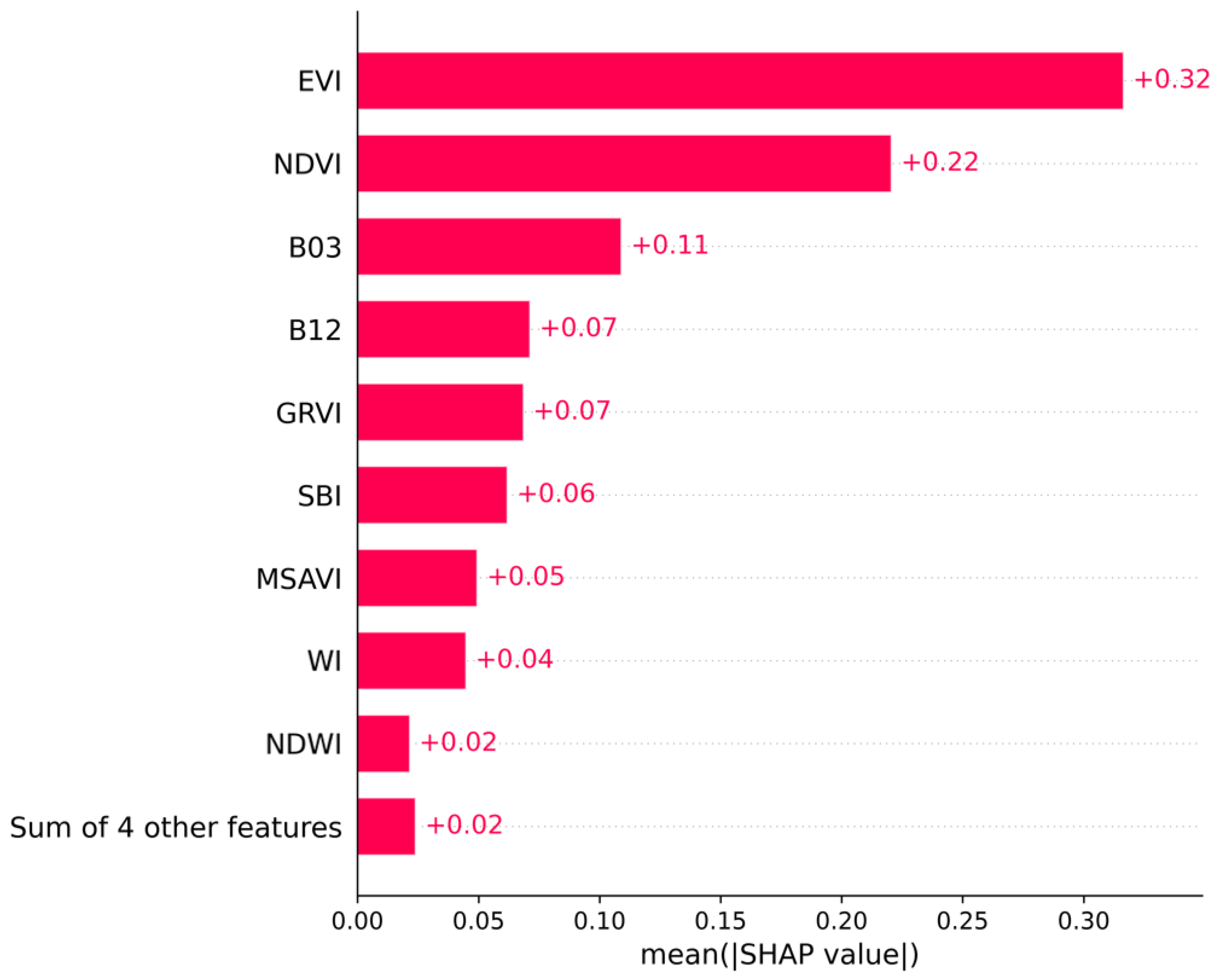
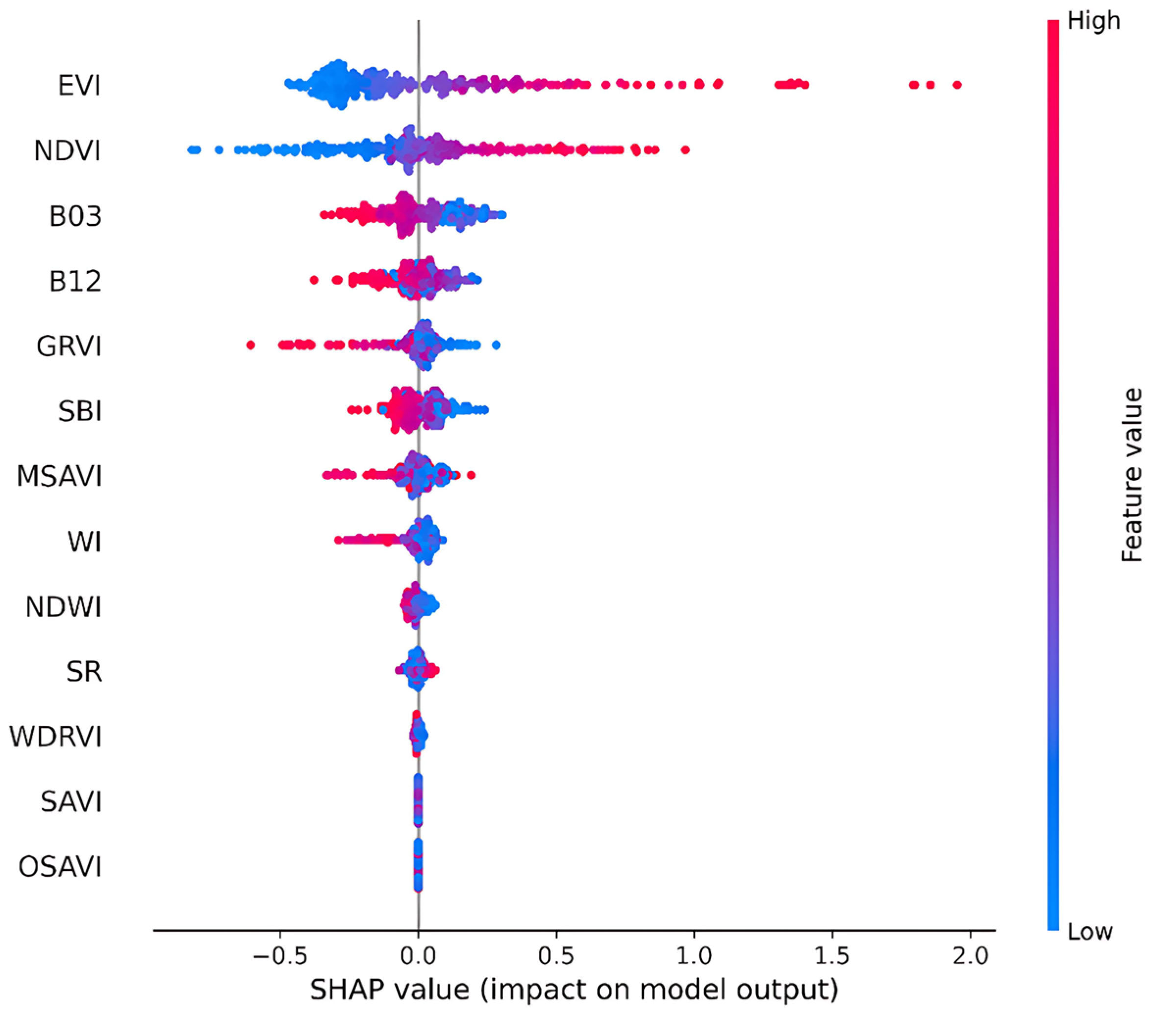
• Model interpretation: An interpretability analysis utilizing SHAP values is then performed on the most accurate ML model to identify the factors affecting individual predictions.

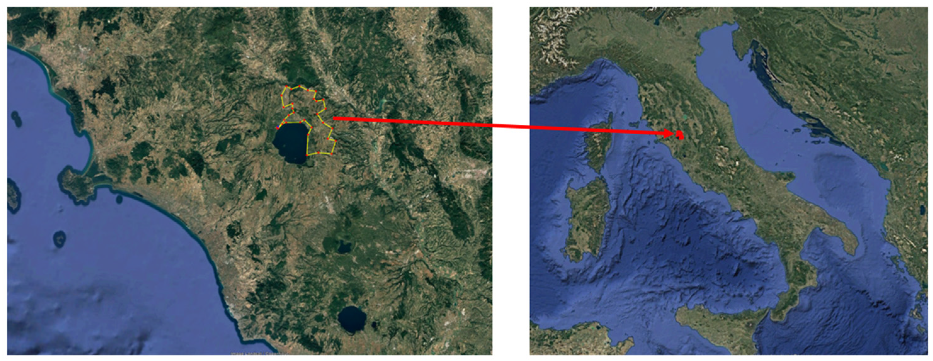
2.1. Data Acquisition

2.1.1. Ground-Truth Crop Yield Data

The study area comprises lupin cultivation fields, with a total area ranging from 0.25 ha to 18.03 ha (average area = 7.64 ha), located in the northern region of the Viterbo province, called Alto Lazio or Tuscia, in Italy. As depicted in Figure 1, this area lies north of the volcanic lake Bolsena (42.66° N, 11.95° E) at an altitude of approximately 312 m above sea level. The region is characterized by a temperate Mediterranean climate, with an average annual temperature of 15.9 °C and average annual precipitation totaling 676.4 mm during the 2023–2024 growing season.

Ground-based measurements taken throughout the harvest season provided the crop yield data used in this investigation in tons per hectare (t/ha). Accurate geolocation and temporal synchronization with satellite data were ensured by spatially referencing the harvested area and aggregating yield values at the field level. These field-measured yield values served as the ground truth for ML model training and testing.

2.1.2. Remote Sensing Data: Sentinel-2 Spectral Bands

Spectral reflectance data were acquired from the Sentinel-2 satellite constellation provided by the European Space Agency (ESA). In particular, surface reflectance values were extracted for the following nine spectral bands, each with a spatial resolution of 20 m, which are useful for monitoring the health of the vegetation:

• $B02$ (Blue, 490 nm);
• $B03$ (Green, 560 nm);
• $B04$ (Red, 665 nm);
• $B05$ (Red Edge 1, 705 nm);
• $B06$ (Red Edge 2, 740 nm);
• $B07$ (Red Edge 3, 783 nm);
• $B8A$ (Narrow Near-Infrared, 865 nm);
• $B11$ (Short-Wave Infrared 1, 1610 nm);
• $B12$ (Short-Wave Infrared 2, 2190 nm).

For this study, Sentinel-2 Level-2A (L2A) imagery was utilized, which is already pre-processed for radiometric calibration, atmospheric correction, geometric correction, and terrain correction. Sentinel-2 provides a high temporal resolution of approximately five days, allowing frequent observations of the same location, depending on atmospheric conditions [49]. The selected sensing date, 18 June 2024, corresponded to the mid to late pod filling phase of the lupin crop, a critical phenological stage that follows flowering and precedes pod maturation [50]. During this period, the plant intensively translocates assimilates to the developing seeds, a process that strongly influences final yield [44]. Acquiring satellite imagery during this stage is particularly valuable, as spectral responses and VIs derived from the above bands can effectively capture variations in canopy biomass, chlorophyll content, and plant water status, thus, enhancing the predictive power of yield estimation models.

2.2. Feature Selection and Preprocessing

2.2.1. Computation of Vegetation Indices

Using the aforementioned spectral reflectance data, the following 13 VIs were calculated based on the related literature [25,27,33,51,52,53,54]:

$$\mathrm{Enhanced} \mathrm{Vegetation} \mathrm{Index}: EVI=2.5·(B8A-B04)/(B8A+6·B04-7.5 ·B02+1),$$

(1)

$$\mathrm{Green} \mathrm{Difference} \mathrm{Vegetation} \mathrm{Index}: GDVI=B8A-B03,$$

(2)

$$\mathrm{Green} \mathrm{Normalized} \mathrm{Difference} \mathrm{Vegetation}: GNDVI=(B8A-B03)/(B8A+B03),$$

(3)

$$\text{Green-Red} \mathrm{Vegetation} \mathrm{Index}: GRVI=(B03-B04)/(B03+B04),$$

(4)

$$\mathrm{Modified} \text{Soil-Adjusted} \mathrm{Vegetation} \mathrm{Index}: MSAVI=2·B8A+1-\sqrt{{(2·B8A+1)}^2-8·(B8A-B04)}/ 2,$$

(5)

$$\mathrm{Normalized} \mathrm{Difference} \mathrm{Vegetation} \mathrm{Index}: NDVI=(B8A-B04)/(B8A+B04),$$

(6)

$$\mathrm{Normalized} \mathrm{Difference} \mathrm{Water} \mathrm{Index}: NDWI=(B03-B8A)/(B03+B8A),$$

(7)

$$\mathrm{Optimized} \text{Soil-Adjusted} \mathrm{Vegetation} \mathrm{Index}: OSAVI=(B8A-B04)/(B8A+B04+0.16),$$

(8)

$$\text{Soil-Adjusted} \mathrm{Vegetation} \mathrm{Index}: SAVI=\left(\right(B8A-B04)·(1+0.5\left)\right)/(B8A+B04+0.5),$$

(9)

$$\mathrm{Simple} \mathrm{Band} \mathrm{Index}: SBI=B12/B03,$$

(10)

$$\mathrm{Simple} \mathrm{Ratio}: SR=B8A/B04,$$

(11)

$$\mathrm{Water} \mathrm{Index}: WI=(B03+B04)/(B8A+B11),$$

(12)

$$\mathrm{Wide} \mathrm{Dynamic} \mathrm{Range} \mathrm{Vegetation} \mathrm{Index}: WDRVI=(0.1·B8A-B04)/(0.1·B8A+B04).$$

(13)

Each index targets specific aspects of vegetation and contributes to monitor different factors that affect crop yield. In total, the above VIs provide a detailed analysis of crop health, vegetation cover, water stress, and chlorophyll content. Occasionally, they are utilized in conjunction with some of the nine spectral bands listed above, which are frequently employed in the field of agricultural yield prediction, as highlighted in the recent review paper of Muruganantham et al. [55].

2.2.2. Outlier Removal

Outliers can distort model training by skewing important statistical measurements and introducing noise. Hence, they can diverge model predictions from the actual underlying patterns resulting in misleading conclusions. To this end, outlier detection and removal was accomplished via the IQR method. Specifically, data points that substantially deviate from the center distribution are identified as outliers by determining the range between the 25th and 75th percentiles and establishing thresholds which are 1.5 times above the upper quartile and 1.5 times below the lower one [56,57].

2.2.3. Addressing Multicollinearity in the Dataset

For the purpose of addressing the multicollinearity in the dataset, namely identifying redundant independent features that bring similar information about the yield (target variable in this study), highly correlated variables were removed based on defined criteria. In particular, a Spearman correlation matrix was calculated so as to assess the relationships between the variables [58]. Any pair of features with a Spearman correlation coefficient greater than 0.85 was considered highly correlated. Subsequently, only one feature from each was retained. The selection process was driven by the following criteria: (a) In cases where a spectral band was highly correlated with a VI, the later was retained, as information for the spectral bands has already been integrated in VI formulation; (b) When a strong correlation was observed between two spectral bands or between two VIs, the feature with the higher absolute correlation with the target variable was retained, because it presents more predictive relevance. However, in certain instances, two highly correlated features could be retained, as they provide complementary agronomic information critical for accurate yield modeling. Although correlated, such features capture distinct physiological and structural characteristics of the crop canopy that influence yield variability. For example, both $EVI$ and $NDVI$ were preserved despite their correlation, as $EVI$ is more sensitive to canopy structure and reduces soil background noise [59], while $NDVI$ effectively captures overall vegetation vigor [60]. Retaining both indices enriches the model’s ability to reflect complex crop biophysical conditions, thereby enhancing predictive robustness and biological interpretability. Overall, this process ensures that the model requires less computation to converge, prevents overfitting or biased predictions, and makes the model more interpretable.

Figure 2 presents the correlation heatmap summarizing the pairwise Spearman correlation coefficients. Each cell shows the correlation between two features with the color intensity corresponding to the magnitude of the correlation. Based on the aforementioned criteria, 13 input features were considered for the present analysis: 2 spectral bands ($B03, B12$) and 11 VIs ($EVI, GRVI, MSAVI, NDVI, NDWI, OSAVI, SAVI, SBI, SR, WI, WDRVI$).

2.2.4. Normalization of Input Features

A normalization is also required, because the dataset includes features with different scales. Spectral bands, for example, have different ranges than VIs. By transforming features to have a mean equal to 0 and standard deviation equal to 1, it ensures that each feature makes an equal contribution to the model. The normalized value $\mathit{Z}$ of data point $X$ is calculated by:

$$Z={\displaystyle \frac{X-\mu }{\sigma }},$$

(14)

where $\mu$ stands for the mean of the feature and $\sigma$ represents the standard deviation of it. All the input features are normalized as a means of ensuring consistent scaling across variables. However, the target variable (yield) was not normalized, as normalizing the target can distort its interpretability, which is critical for practical applications.

2.2.5. Data Augmentation

Crop yield prediction through the use of remote sensing data usually faces the challenge of imbalanced target distribution, especially when dealing with agricultural datasets collected from fields [19]. Such imbalances can negatively impact the performance of regression models by biasing predictions towards the more frequently occurring yield ranges. In turn, these biased predictions can result in poor generalization and reduced reliability in practical decision-making. To address this issue, SMOTER was implemented, a data augmentation method specifically designed to handle imbalanced regression problems, where the target variable is continuous. Unlike traditional SMOTE, which is designed for classification [61], SMOTER identifies sparse areas in the feature space, selects nearest neighbors, and creates new instances through interpolation while adjusting target values to maintain realistic distributions [62]. In particular, the synthetic target value, $y_i^{new}$, is calculated through:

$$y_i^{new}={\displaystyle \frac{\frac{y_i}{d_1}+\frac{y_i^{nearest}}{d_2}}{\frac{1}{d_1}+\frac{1}{d_2}}},$$

(15)

where $y_i$ is the target value of the data point $x_i$, while $x_i^{nearest}$ is its nearest neighbor with a target value of $y_i^{nearest}$ [63]. The target value of a newly generated point, $x_i^{new}$, is proportional to its Euclidean distance from its parent points, meaning that its value is more influenced by the parent point it is closer to. Moreover, $d_1$ corresponds to the Euclidean distance between $x_i^{new}$ and $x_i,$ while $d_2$ represents the Euclidean distance between $x_i^{new}$, and $x_i^{nearest}$.

Consequently, the SMOTER algorithm methodically balances synthetic sample generation as a means of avoiding over- or under-sampling, therefore, ensuring that the augmented dataset has a more uniform distribution across the target range. This reduces model bias towards over-represented yield levels and improves prediction accuracy for rare or extreme yield values. SMOTER also incorporates mechanisms to limit the creation of unrealistic synthetic points by restricting interpolation within defined boundaries. Overall, the integration of SMOTER into the preprocessing pipeline ensured that the ML models were better equipped to handle heterogeneity in the yield data as well as minimized the risk of overfitting to dominant target ranges.

2.3. Machine Learning Used for Yield Prediction

2.3.1. Tested Machine Learning Algorithms

In order to predict crop yield based on spectral bands and VIs, six ML algorithms were employed, demonstrating different modeling techniques: (a) tree-based (Decision Tree (DT), Extreme Gradient Boosting (XGBoost), Random Forest (RF)); (b) distance-based (K-Nearest Neighbors (KNN)); (c) kernel-based (Support Vector Regressor (SVR)); and (d) neural network-based (Multi-Layer Perceptron Regressor (MLPR)) models.

In short, tree-based models were particularly useful, because of their inherent feature importance estimation, while KNN offered a simple, efficient distance-based approach for localized yield prediction. SVR, leveraging the kernel-based optimization, had the ability to model high-dimensional nonlinear interactions, while MLPR explored DL capabilities in learning complex patterns from VIs and spectral inputs. The diversity of these algorithms facilitated a thorough assessment of the models’ predictive accuracy and their ability to generalize effectively to unseen crop yield data.

2.3.2. Performance Metrics

The scikit-learn’s GridSearchCV (version 1.6.1) was implemented towards optimizing hyperparameters for the ML models. Also, five-fold cross-validation was used, along with data shuffles to guarantee randomness [64,65]. To assess overall performance, the following commonly used indicators were averaged after the cross-validation process was finished:

$$MAE={\displaystyle \frac{\sum _{i=1}^n\left|y_i-{\widehat{y}}_i\right|}{n}},$$

(16)

$$MSE={\displaystyle \frac{\sum _{i=1}^n{(y_i-{\widehat{y}}_i)}^2}{n}},$$

(17)

$$RMS=\sqrt{{\displaystyle \frac{\sum _{i=1}^n{(y_i-{\widehat{y}}_i)}^2}{n}}},$$

(18)

$$R^2=1-{\displaystyle \frac{\sum _{i=1}^n{(y_i-{\widehat{y}}_i)}^2}{\sum _{i=1}^n{(y_i-\overline{y})}^2}}.$$

(19)

In Equations (16)–(19), $n$ signifies the total count of data points,${\widehat{y}}_i$ and $y_i$ correspond to the predicted and actual values of the $i^{th}$ data point, respectively. Finally, $\overline{y}$ denotes the mean of the actual values, while $y_{min}$ and $y_{max}$ stand for the minimum and maximum values of the actual data, respectively. $R^2$ provides a measure of how well the model explains the variance in crop yield. The error-based metrics used in this study, namely $MAE$, $MSE$, and $RMS$, capture the magnitude of prediction errors. Overall, by using both variance-based and error-based metrics, along with rigorous cross-validation and hyperparameter optimization, the study provides a reliable assessment of the crop yield prediction models.

2.4. Model Interpretation

The significance of interpretability arises from the fact that the prediction itself is often insufficient in real-world circumstances, such as agricultural ones. Doshi-Velez and Kim [66] stressed that knowing what the model predicts is not always enough. Understanding the model’s reasoning for making that prediction holds equal importance to answering the underlying query or decision-making need. Interpretability fills this gap, by providing insights into the model’s reasoning, promoting informed decision-making, responsibility, and trust in precision agriculture [67].

In the present framework, SHAP was implemented (SHAP Python library, version 0.47.2) to improve interpretability by quantifying each feature’s contribution to the ML model’s output. This analysis was applied only to the most accurate ML model identified in this study to understand the relative importance of spectral bands and VIs in crop yield prediction. Specifically, the present analysis used TreeSHAP, a customized version of SHAP for tree-based models [68]. Although calculating SHAP values can be computationally costly, this specialized variant offers an efficient technique by utilizing conditional expectancies and processing all feature combinations within the tree structure. TreeSHAP computes SHAP values in polynomial rather than exponential time by taking advantage of the hierarchical nature of tree-based models. This makes it practical for complex datasets. TreeSHAP evaluates the marginal contribution of each feature along all paths of a decision tree. It does so by comparing the model’s output for a specific instance against a baseline expectation, iterating through the tree structure. Three important properties are satisfied by the local feature importance values: (a) SHAP values are designed such that their sum corresponds exactly to the model’s prediction; (b) Features that are not utilized by the model contribute nothing to its prediction, as their corresponding SHAP values are zero; and (c) A feature’s SHAP value does not decrease as its contribution increases [46].

3. Results

3.1. Comparison of Machine Learning Performance

As elaborated in Section 2.3.2, for each ML model hyperparameter, tuning took place through GridSearchCV, guaranteeing the best possible performance configurations. Towards assessing the predictive capability of the developed ML models, namely DT, XGBoost, RF, KNN, SVR, and MLPR, a comparative analysis was implemented using key evaluation metrics. Figure 3a–f depict scatter plots that compare the predicted crop yields against the actual values regarding the six ML models on the test dataset to illustrate generalization performance. Among them, XGBoost succeeded the highest $R^2$ score (0.8756), demonstrating the strongest predictive performance, followed by MLPR ($R^2=$ 0.8141), and SVR ($R^2=0$.7933). This ML regressors’ exceptional performance can be ascribed to their capacity to effectively capture non-linear correlations in high-dimensional data. Specifically, XGBoost outperformed the other models, because of its ensemble boosting framework that creates a powerful predictive model by combining several weak learners. It also integrates regularization to avoid overfitting and is optimized for both accuracy and speed [69].

In addition, MLPR, exploiting its multi-layer architecture is able to capture complex patterns in the data [70], which is particularly beneficial in this analysis where interactions among spectral bands and VIs are often non-linear [20]. As far as SVR is concerned, it maps input features into higher-dimensional spaces using kernel functions. This enables SVR to model complex relationships in the data, while emphasizing minimizing generalization error. This renders it resilient to overfitting. On the other hand, more scattered predictions were observed for KNN ($R^2=0.6987$) and RF ($R^2=0.6959$), with DT exhibiting the lowest predictive performance ($R^2=0.6393$). The poorest performance of DT can be attributed to the restrictions of single decision trees that lack generalization capability and have propensity to overfit training data [71].

For each of the six ML models, the evaluation metrics are summarized in

Table 1. Evaluation metrics of the utilized machine learning models; the best values in each column are highlighted in bold.

Algorithm	$\mathit{M}\mathit{A}\mathit{E}$	$\mathit{M}\mathit{S}\mathit{E}$	$\mathit{R}\mathit{M}\mathit{S}$	${\mathit{R}}^2$
DT	0.3297	0.1970	0.4438	0.6393
XGBoost	0.2399	0.1149	0.3389	0.8756
RF	0.2900	0.1661	0.4076	0.6959
SVR	0.2404	0.1129	0.3360	0.7933
KNN	0.2624	0.1646	0.4057	0.6987
MLPR	0.2467	0.1125	0.3354	0.8141

DT: Decision Tree; KNN: K-Nearest Neighbors; MLPR: Multi-Layer Perceptron Regressor; RF: Random Forest; SVR: Support Vector Regressor; XGBoost; Extreme Gradient Boosting.

. Note that for $MAE$, $MSE$, and $RMS$, lower values indicate better performance, whereas for $R^2$, higher values indicate better performance. With the lowest $MAE$ (0.2399), low $MSE$ (0.1149), and $RMSE$ (0.3389) as well as the highest $R^2$ score mentioned above, XGBoost performed better than the other regressors. These values demonstrate its great capability to effectively estimate the relationship between remote sensing-related variables and crop yield. With $R^2$ values approximately equal to 0.8, both MLPR and SVR showed competitive performance, signifying their capacity to capture nonlinear interactions. KNN and RF performed moderately well, but their lower $R^2$ values (~0.7) showed that their predictions were less accurate than those of XGBoost. Finally, the DT model produced the weakest results on all metrics, indicating the limitations of its single-tree structure.

3.2. SHAP-Based Interpretation of XGBoost Feature Contributions

To understand the general patterns of feature influence on crop yield predictions made by the ML model showing the best performance, namely XGBoost, this section focuses on global interpretability using SHAP values. As this model is an ensemble of decision trees, TreeSHAP can accurately identify the most influential features driving predictions. To this end, a SHAP summary plot is provided in Figure 4, which shows the most influential features by summarizing the mean absolute SHAP values. The higher the SHAP value the greater the contribution of that feature to increasing the ML model’s prediction. In short, $EVI$ was found to be the most important feature, displaying the highest mean absolute SHAP value of approximately 0.32, followed by $NDVI$ with a mean absolute SHAP value of 0.22.

This plot highlights also the importance of the green ($B03$) and short-wave infrared ($B12$) spectral bands among the most influential features for crop yield prediction. VIs, like $GRVI$ and $SBI$, also demonstrated remarkable importance. Other indices, including $MSAVI$, $WI$, and $NDWI$ in descending order of mean absolute SHAP value, showed moderate contributions. The sum of the four other features ($OSAVI$, $SAVI$, $SR$, and $WDRVI$) has a combined mean absolute SHAP value of 0.02. This signifies that the individual contributions of these features are relatively small in comparison to the top nine features.

In order to get more information about not only the feature’s importance but also the distribution of how much that feature influences each prediction, a beeswarm plot is provided in Figure 5. This helps towards determining whether characteristics consistently affect predictions in a positive or negative way across samples. The horizontal positioning of each dot, representing a distinct data point, indicates the SHAP value, which shows the extent to which that attribute increased or decreased the model’s prediction for that particular instance. While features with narrower distributions often have a more uniform but lesser influence, those with wider distributions appear to have a larger and more varied impact on crop yield estimates. Furthermore, the concentration of data points with comparable levels of influence is shown when dots cluster vertically around a specific SHAP value. Focusing on Figure 5, high values of both $EVI$ and $NDVI$ (red circles) exhibited a positive correlation with lupin yield (pushing the prediction higher). In contrast, low values (blue circles) are associated with negative SHAP values (pushing the prediction lower). This pattern is consistent with the known agronomic roles of $EVI$ and $NDVI$ as indicators of vegetation vigor, canopy density, and chlorophyll content, which are key drivers of biomass accumulation in legumes [8,44]. The observed positive relationship reinforces the interpretation that increased vegetative development during the mid-season is strongly linked to enhanced yield potential.

On the other hand, high values of the green and short-wave infrared spectral bands demonstrate an almost negative correlation with the predicted crop yield. Consequently, higher reflectance in these portions of the spectrum tends to decrease the model’s prediction of crop yield. $GRVI$, $SBI$, $MSAVI$, and $WI$ show a less consistently negative correlation with the predicted crop yield. Therefore, while high values of these VIs tend to be associated with lower predicted yields, this negative association is not strong and can vary across different data points. The rest of the VIs show a more concentrated distribution of SHAP values around zero, which suggests a minimal impact on the model’s predictions. Besides, the color gradients cannot provide clear understandings into the direction of their influence, since blue and red are seen across both negative and positive SHAP values.

4. Discussion

The present study initially assessed the predictive performance of six distinct ML models, namely DT, XGBoost, RF, KNN, SVR, and MLPR in the context of crop yield prediction using remote sensing data. In brief, XGBoost demonstrated superior performance, achieving the highest $R^2$ score (0.8756), and low errors, while MLPR and SVR had competitive, yet lower performance. This finding supports recent studies stressing the strength of gradient-boosted decision tree ensembles when dealing with high-dimensional, non-linear data, especially when combined with hyperparameter optimization techniques [72,73,74]. This strength was particularly advantageous in this analysis dealing with remote sensing data, where interactions between VIs and spectral bands are complex.

In addition to predictive accuracy, SHAP analysis was used to enhance model interpretability in the best-performing ML model. SHAP can also address correlated features by distributing the importance (Shapley values) between them based on their marginal contributions across all possible coalitions of features [75]. This means that if two features are highly correlated and provide similar information to the model, SHAP will attribute the “credit” for their joint contribution in a fair, game-theoretic manner, rather than assigning all importance to just one of them. This leads to more reliable interpretations, especially in agriculture, where spectral bands and vegetation indices often exhibit strong interdependencies.

In the current analysis, a high-level overview was accomplished concerning which variables consistently affect crop yield predictions, allowing us to reveal general agronomic patterns like the strong role of $EVI$ and $NDVI$. This is attributed to the fact that both indices serve as proxies for plant health, vigor, and photosynthetic activity. These are central physiological processes which directly influence biomass accumulation and yield formation. In the case of lupin, a leguminous crop that relies on effective canopy development and nitrogen fixation for optimal productivity, higher $NDVI$ and $EVI$ values typically reflect healthy, actively growing plants with dense foliage, adequate nutrient status, and minimal stress. They integrate spectral responses from red and near-infrared bands (in the case of $NDVI$) or add blue band correction (in the case of $EVI$), enhancing sensitivity to chlorophyll content and structural canopy characteristics. As a consequence, their prominence in the model is not only statistically significant, but also agronomically meaningful. This observation qualitatively aligns with simple regression analyses, where crop yield models using $NDVI$ often show an exponential increase with the latter [76,77]. Moreover, Son et al. [78] highlighted that $EVI$-based models provided slightly more precise yield estimates compared to those based on $NDVI$.

Denser foliage is associated with higher values of $EVI$ and $NDVI$, which reflect greater photosynthetic activity and biomass accumulation, ultimately leading to higher yield. In contrast, the green spectral band ($B03$) exhibits a more complex response at high canopy densities. Reflectance saturation, where spectral indices or bands lose sensitivity at high biomass levels, is a well-recognized challenge in remote sensing of vegetation [79]. Thus, during the mid to late pod filling phase, the dense lupin canopy can lead to reflectance saturation or even a slight decrease in $B03$. This phenomenon is primarily driven by increased self-shadowing and complex internal light scattering within the thick canopy, rather than photosynthetic absorption of green wavelengths. Consequently, lower $B03$ values in this mature stage probably indicate a highly developed canopy, correlating with maximized yield. In high-yielding lupin crops, denser foliage absorbs also more red light for photosynthesis [80], reducing reflectance in this band that is strongly associated with chlorophyll absorption. A negative correlation between $B12$ (SWIR band) reflectance and crop yield was also observed. This can be attributed to its sensitivity to plant water content. Healthy, well-watered lupin crops absorb more SWIR light, resulting in lower $B12$ reflectance [81], suggesting higher yield potential.

In this fashion, the limitations of the present study should be mentioned. First, the performance of the ML models was assessed using a dataset within a specific geographical and climatic context, namely the Mediterranean. This may limit the generalizability of the outcomes to other regions that have different environmental conditions. Moreover, the Spearman correlation analysis, utilized to remove redundant features, although a common data preprocessing step [82,83], it may come with potential disadvantages. Indicatively, there is a risk that aspects that may otherwise provide complementing information in non-linear models will be lost. Despite its disadvantages, the use of this analysis offers notable advantages, particularly in reducing multicollinearity and dimensionality, which can enhance both model interpretability and computational efficiency. This is of central importance as it supports the practical usability and scalability of ML-based solutions in real-world agricultural settings. Meanwhile, faster model deployment and training are made possible by increased computational efficiency, particularly when working with large remote sensing datasets or incorporating the model into time-sensitive decision-making pipelines [84]. Besides, although remote sensing-based features such as spectral bands and VIs are considered a valid input [40,85], the study did not include other important agronomic variables like soil properties, which could influence yield outcomes.

Based on the findings of this study and towards addressing the aforementioned limitations, improving model generalizability through its validation across several geographic locations and climatic conditions should be the prioritized in future research. Additionally, incorporating multi-temporal satellite imagery could enhance the model’s ability to capture dynamic crop growth patterns and improve the robustness of yield predictions. In order to reduce the need for large amounts of labeled data, future research could also examine active learning strategies, where the model selectively requests the most informative data points to be labeled [86,87]. Furthermore, incorporating a wider range of agronomic variables could improve the model’s ability to capture critical interactions that affect yield, like soil fertility, irrigation practices, and pest management.

5. Conclusions

This study presents a novel and interpretable ML framework for crop yield prediction, with a specific focus on an understudied legume crop such lupin. By integrating Sentinel-2 remote sensing data with precisely georeferenced yield data, we assessed the predictive performance of tree-, kernel-, and neural network-based ML algorithms. A thorough data preprocessing pipeline was set up to ensure high-quality data suitable for effective model training. This encompassed steps such as calculation of VIs based on spectral reflectance information, outlier removal using the IQR method, identification and handling of highly correlated features through Spearman analysis, and Z-score normalization. In the direction of addressing potential data imbalance, the SMOTER technique was also applied. Subsequently, six ML models were trained, with hyperparameter optimization and rigorous performance evaluation using GridSearchCV and 5-fold cross-validation.

It is concluded that the most effective ML model for the present dataset was XGBoost with an $R^2=$ 0.8756 and robust performance across all evaluation metrics. MLPR and SVR demonstrated comparable but less effective predictive performance with $R^2$ equal to 0.8141 and 0.7933, respectively. In an effort to gain a clearer understanding of the model’s decision-making process, an interpretability analysis was conducted on the developed XGBoost model using SHAP. Global interpretability highlighted $EVI$ and $NDVI$ as well as two specific spectral bands ($B03$, $B12$) as consistently influential predictors of crop yield.

In summary, by integrating remote sensing data with XAI techniques the study not only achieved high predictive accuracy, but also offered transparent and interpretable insights into the drivers of crop yield variability. This dual focus addresses a critical barrier in agricultural ML adoption, namely trust and actionable relevance, enabling data-driven decisions that are both scientifically grounded and practically relevant. Future work should focus on validating the model across diverse regions as well as including agronomic variables for a more detailed view of yield drivers. Combining expert input with active learning could also improve model development while minimizing labeling efforts.

References

1. Matthews, L.; Strauss, J.A.; Reinsch, T.; Smit, H.P.J.; Taube, F.; Kluss, C.; Swanepoel, P.A. Legumes and livestock in no-till crop rotations: Effects on nitrous oxide emissions, carbon sequestration, yield, and wheat protein content. Agric. Syst. 2025, 224, 104218. [Google Scholar] [CrossRef]
2. Liu, R.; Flanagan, B.M.; Ratanpaul, V.; Gidley, M.J. Valorising legume protein extraction side-streams: Isolation and characterisation of fibre-rich and starch-rich co-products from wet fractionation of five legumes. Food Hydrocoll. 2025, 164, 111191. [Google Scholar] [CrossRef]
3. Dela, M.; Shanka, D.; Dalga, D. Biofertilizer and NPSB fertilizer application effects on nodulation and productivity of common bean (Phaseolus vulgaris L.) at Sodo Zuria, Southern Ethiopia. Open Life Sci. 2023, 18, 20220537. [Google Scholar] [CrossRef]
4. Folina, A.; Stavropoulos, P.; Mavroeidis, A.; Roussis, I.; Kakabouki, I.; Tsiplakou, E.; Bilalis, D. Optimizing Fodder Yield and Quality Through Grass–Legume Relay Intercropping in the Mediterranean Region. Plants 2025, 14, 877. [Google Scholar] [CrossRef]
5. Tita, D.; Mahdi, K.; Devkota, K.P.; Devkota, M. Climate change and agronomic management: Addressing wheat yield gaps and sustainability challenges in the Mediterranean and MENA regions. Agric. Syst. 2025, 224, 104242. [Google Scholar] [CrossRef]
6. Benos, L.; Makaritis, N.; Kolorizos, V. From Precision Agriculture to Agriculture 4.0: Integrating ICT in Farming—Information and Communication Technologies for Agriculture—Theme III: Decision; Bochtis, D.D., Sørensen, C.G., Fountas, S., Moysiadis, V., Pardalos, P.M., Eds.; Springer International Publishing: Cham, Switzerland, 2022; pp. 79–93. ISBN 978-3-030-84152-2. [Google Scholar]
7. Filippi, P.; Han, S.Y.; Bishop, T.F.A. On crop yield modelling, predicting, and forecasting and addressing the common issues in published studies. Precis. Agric. 2024, 26, 8. [Google Scholar] [CrossRef]
8. Parashar, N.; Johri, P.; Khan, A.A.; Gaur, N.; Kadry, S. An Integrated Analysis of Yield Prediction Models: A Comprehensive Review of Advancements and Challenges. Comput. Mater. Contin. 2024, 80, 389–425. [Google Scholar] [CrossRef]
9. Petropoulos, T.; Benos, L.; Busato, P.; Kyriakarakos, G.; Kateris, D.; Aidonis, D.; Bochtis, D. Soil Organic Carbon Assessment for Carbon Farming: A Review. Agriculture 2025, 15, 567. [Google Scholar] [CrossRef]
10. Cheng, E.; Zhang, B.; Peng, D.; Zhong, L.; Yu, L.; Liu, Y.; Xiao, C.; Li, C.; Li, X.; Chen, Y.; et al. Wheat yield estimation using remote sensing data based on machine learning approaches. Front. Plant Sci. 2022, 13, 1090970. [Google Scholar] [CrossRef]
11. Weiss, M.; Jacob, F.; Duveiller, G. Remote sensing for agricultural applications: A meta-review. Remote Sens. Environ. 2020, 236, 111402. [Google Scholar] [CrossRef]
12. Darra, N.; Anastasiou, E.; Kriezi, O.; Lazarou, E.; Kalivas, D.; Fountas, S. Can Yield Prediction Be Fully Digitilized? A Systematic Review. Agronomy 2023, 13, 567. [Google Scholar] [CrossRef]
13. Jiang, H.; Jiang, L.; He, L.; Murengami, B.G.; Jing, X.; Misiewicz, P.A.; Cheein, F.A.; Fu, L. Yield prediction of root crops in field using remote sensing: A comprehensive review. Comput. Electron. Agric. 2024, 227, 109600. [Google Scholar] [CrossRef]
14. Ali, A.M.; Abouelghar, M.; Belal, A.A.; Saleh, N.; Yones, M.; Selim, A.I.; Amin, M.E.S.; Elwesemy, A.; Kucher, D.E.; Maginan, S.; et al. Crop Yield Prediction Using Multi Sensors Remote Sensing (Review Article). Egypt. J. Remote Sens. Sp. Sci. 2022, 25, 711–716. [Google Scholar] [CrossRef]
15. Kasampalis, D.A.; Alexandridis, T.K.; Deva, C.; Challinor, A.; Moshou, D.; Zalidis, G. Contribution of Remote Sensing on Crop Models: A Review. J. Imaging 2018, 4, 52. [Google Scholar] [CrossRef]
16. Nearing, G.S.; Crow, W.T.; Thorp, K.R.; Moran, M.S.; Reichle, R.H.; Gupta, H.V. Assimilating remote sensing observations of leaf area index and soil moisture for wheat yield estimates: An observing system simulation experiment. Water Resour. Res. 2012, 48, W05525. [Google Scholar] [CrossRef]
17. Li, Z.; Wang, J.; Xu, X.; Zhao, C.; Jin, X.; Yang, G.; Feng, H. Assimilation of Two Variables Derived from Hyperspectral Data into the DSSAT-CERES Model for Grain Yield and Quality Estimation. Remote Sens. 2015, 7, 12400–12418. [Google Scholar] [CrossRef]
18. Clevers, J.; Vonder, O.; Jongschaap, R.; Desprats, J.F.; King, C.; Prévot, L.; Bruguier, N. Using SPOT data for calibrating a wheat growth model under mediterranean conditions. Agronomie 2002, 22, 687–694. [Google Scholar] [CrossRef]
19. Joshi, A.; Pradhan, B.; Gite, S.; Chakraborty, S. Remote-Sensing Data and Deep-Learning Techniques in Crop Mapping and Yield Prediction: A Systematic Review. Remote Sens. 2023, 15, 2014. [Google Scholar] [CrossRef]
20. Meghraoui, K.; Sebari, I.; Pilz, J.; Ait El Kadi, K.; Bensiali, S. Applied Deep Learning-Based Crop Yield Prediction: A Systematic Analysis of Current Developments and Potential Challenges. Technologies 2024, 12, 43. [Google Scholar] [CrossRef]
21. Peng, D.; Zhou, L.; Huang, J.; Zhou, B.; Wang, F. Rice yield estimation based on MODIS EVI and measured data derived from statistical sampling plots at province level. Nongye Gongcheng Xuebao/Trans. Chin. Soc. Agric. Eng. 2011, 27, 106–114. [Google Scholar] [CrossRef]
22. Bazzi, H.; Ciais, P.; Makowski, D.; Baghdadi, N. Advancing winter wheat yield anomaly prediction with high-resolution satellite-based gross primary production. One Earth 2025, 8, 101146. [Google Scholar] [CrossRef]
23. Wang, Y.; Feng, K.; Sun, L.; Xie, Y.; Song, X.-P. Satellite-based soybean yield prediction in Argentina: A comparison between panel regression and deep learning methods. Comput. Electron. Agric. 2024, 221, 108978. [Google Scholar] [CrossRef]
24. Ashfaq, M.; Khan, I.; Alzahrani, A.; Tariq, M.U.; Khan, H.; Ghani, A. Accurate Wheat Yield Prediction Using Machine Learning and Climate-NDVI Data Fusion. IEEE Access 2024, 12, 40947–40961. [Google Scholar] [CrossRef]
25. You, J.; Li, X.; Low, M.; Lobell, D.; Ermon, S. Deep Gaussian Process for Crop Yield Prediction Based on Remote Sensing Data. In Proceedings of the AAAI Conference on Artificial Intelligence, San Francisco, CA, USA, 4–9 February 2017; Volume 31. [Google Scholar] [CrossRef]
26. Kuwata, K.; Shibasaki, R. Estimating crop yields with deep learning and remotely sensed data. In Proceedings of the 2015 IEEE International Geoscience and Remote Sensing Symposium (IGARSS), Milan, Italy, 26–31 July 2015; pp. 858–861. [Google Scholar]
27. Wolanin, A.; Mateo-García, G.; Camps-Valls, G.; Gómez-Chova, L.; Meroni, M.; Duveiller, G.; Liangzhi, Y.; Guanter, L. Estimating and understanding crop yields with explainable deep learning in the Indian Wheat Belt. Environ. Res. Lett. 2020, 15, 24019. [Google Scholar] [CrossRef]
28. Cao, J.; Zhang, Z.; Luo, Y.; Zhang, L.; Zhang, J.; Li, Z.; Tao, F. Wheat yield predictions at a county and field scale with deep learning, machine learning, and google earth engine. Eur. J. Agron. 2021, 123, 126204. [Google Scholar] [CrossRef]
29. Tian, H.; Wang, P.; Tansey, K.; Zhang, J.; Zhang, S.; Li, H. An LSTM neural network for improving wheat yield estimates by integrating remote sensing data and meteorological data in the Guanzhong Plain, PR China. Agric. For. Meteorol. 2021, 310, 108629. [Google Scholar] [CrossRef]
30. Tian, H.; Wang, P.; Tansey, K.; Han, D.; Zhang, J.; Zhang, S.; Li, H. A deep learning framework under attention mechanism for wheat yield estimation using remotely sensed indices in the Guanzhong Plain, PR China. Int. J. Appl. Earth Obs. Geoinf. 2021, 102, 102375. [Google Scholar] [CrossRef]
31. Ma, Y.; Zhang, Z.; Kang, Y.; Özdoğan, M. Corn yield prediction and uncertainty analysis based on remotely sensed variables using a Bayesian neural network approach. Remote Sens. Environ. 2021, 259, 112408. [Google Scholar] [CrossRef]
32. Xie, Y.; Huang, J. Integration of a Crop Growth Model and Deep Learning Methods to Improve Satellite-Based Yield Estimation of Winter Wheat in Henan Province, China. Remote Sens. 2021, 13, 4372. [Google Scholar] [CrossRef]
33. Fernandes, J.L.; Ebecken, N.F.F.; Esquerdo, J.C.D.M. Sugarcane yield prediction in Brazil using NDVI time series and neural networks ensemble. Int. J. Remote Sens. 2017, 38, 4631–4644. [Google Scholar] [CrossRef]
34. Li, Y.; Li, R.; Ji, R.; Wu, Y.; Chen, J.; Wu, M.; Yang, J. Research on Factors Affecting Global Grain Legume Yield Based on Explainable Artificial Intelligence. Agriculture 2024, 14, 438. [Google Scholar] [CrossRef]
35. Manafifard, M. A new hyperparameter to random forest: Application of remote sensing in yield prediction. Earth Sci. Inform. 2024, 17, 63–73. [Google Scholar] [CrossRef]
36. Ishaq, R.A.F.; Zhou, G.; Jing, G.; Shah, S.R.A.; Ali, A.; Imran, M.; Jiang, H. Obaid-ur-Rehman Geospatial Robust Wheat Yield Prediction Using Machine Learning and Integrated Crop Growth Model and Time-Series Satellite Data. Remote Sens. 2025, 17, 1140. [Google Scholar] [CrossRef]
37. Joshi, A.; Pradhan, B.; Chakraborty, S.; Varatharajoo, R.; Gite, S.; Alamri, A. Deep-Transfer-Learning Strategies for Crop Yield Prediction Using Climate Records and Satellite Image Time-Series Data. Remote Sens. 2024, 16, 4804. [Google Scholar] [CrossRef]
38. Zhao, Y.; He, J.; Yao, X.; Cheng, T.; Zhu, Y.; Cao, W.; Tian, Y. Wheat Yield Robust Prediction in the Huang-Huai-Hai Plain by Coupling Multi-Source Data with Ensemble Model under Different Irrigation and Extreme Weather Events. Remote Sens. 2024, 16, 1259. [Google Scholar] [CrossRef]
39. Jeong, S.; Ko, J.; Ban, J.; Shin, T.; Yeom, J. Deep learning-enhanced remote sensing-integrated crop modeling for rice yield prediction. Ecol. Inform. 2024, 84, 102886. [Google Scholar] [CrossRef]
40. Benos, L.; Tagarakis, A.C.; Dolias, G.; Berruto, R.; Kateris, D.; Bochtis, D. Machine Learning in Agriculture: A Comprehensive Updated Review. Sensors 2021, 21, 3758. [Google Scholar] [CrossRef]
41. Qin, X.; Wu, B.; Zeng, H.; Zhang, M.; Tian, F. Global Gridded Crop Production Dataset at 10 km Resolution from 2010 to 2020. Sci. Data 2024, 11, 1377. [Google Scholar] [CrossRef] [PubMed]
42. Li, X.; Qu, Y.; Geng, H.; Xin, Q.; Huang, J.; Peng, S.; Zhang, L. Mapping annual 10-m maize cropland changes in China during 2017–2021. Sci. Data 2023, 10, 765. [Google Scholar] [CrossRef]
43. Wuyun, D.; Sun, L.; Chen, Z.; Li, Y.; Han, M.; Shi, Z.; Ren, T.; Zhao, H. A 10-meter resolution dataset of abandoned and reclaimed cropland from 2016 to 2023 in Inner Mongolia, China. Sci. Data 2025, 12, 317. [Google Scholar] [CrossRef]
44. Nuttall, J.G.; Wallace, A.J.; Delahunty, A.J.; Perry, E.M.; Clancy, A.B.; Panozzo, J.F.; Fitzgerald, G.J.; Walker, C.K. Lentil grain quality and segregation opportunities in-field using remote sensing. Agron. J. 2024, 116, 121–140. [Google Scholar] [CrossRef]
45. Das, P.; Jha, G.K.; Lama, A.; Parsad, R. Crop Yield Prediction Using Hybrid Machine Learning Approach: A Case Study of Lentil (Lens culinaris Medik.). Agriculture 2023, 13, 596. [Google Scholar] [CrossRef]
46. Molnar, C. Interpretable Machine Learning: A Guide for Making Black Box Models Explainable, 3rd ed.; 2025. Available online: https://christophm.github.io/interpretable-ml-book/ (accessed on 10 June 2025).
47. Ryo, M. Explainable artificial intelligence and interpretable machine learning for agricultural data analysis. Artif. Intell. Agric. 2022, 6, 257–265. [Google Scholar] [CrossRef]
48. Benos, L.; Tsaopoulos, D.; Tagarakis, A.C.; Kateris, D.; Busato, P.; Bochtis, D. Explainable AI-Enhanced Human Activity Recognition for Human–Robot Collaboration in Agriculture. Appl. Sci. 2025, 15, 650. [Google Scholar] [CrossRef]
49. Drusch, M.; Del Bello, U.; Carlier, S.; Colin, O.; Fernandez, V.; Gascon, F.; Hoersch, B.; Isola, C.; Laberinti, P.; Martimort, P.; et al. Sentinel-2: ESA’s Optical High-Resolution Mission for GMES Operational Services. Remote Sens. Environ. 2012, 120, 25–36. [Google Scholar] [CrossRef]
50. Bebeli, P.J.; Lazaridi, E.; Chatzigeorgiou, T.; Suso, M.-J.; Hein, W.; Alexopoulos, A.A.; Canha, G.; van Haren, R.J.F.; Jóhannsson, M.H.; Mateos, C.; et al. State and Progress of Andean Lupin Cultivation in Europe: A Review. Agronomy 2020, 10, 1038. [Google Scholar] [CrossRef]
51. Jiménez-Jiménez, S.I.; Marcial-Pablo, M.d.J.; Ojeda-Bustamante, W.; Sifuentes-Ibarra, E.; Inzunza-Ibarra, M.A.; Sánchez-Cohen, I. VICAL: Global Calculator to Estimate Vegetation Indices for Agricultural Areas with Landsat and Sentinel-2 Data. Agronomy 2022, 12, 1518. [Google Scholar] [CrossRef]
52. Jeong, S.; Ko, J.; Yeom, J.-M. Predicting rice yield at pixel scale through synthetic use of crop and deep learning models with satellite data in South and North Korea. Sci. Total Environ. 2022, 802, 149726. [Google Scholar] [CrossRef]
53. Yang, W.; Nigon, T.; Hao, Z.; Dias Paiao, G.; Fernández, F.G.; Mulla, D.; Yang, C. Estimation of corn yield based on hyperspectral imagery and convolutional neural network. Comput. Electron. Agric. 2021, 184, 106092. [Google Scholar] [CrossRef]
54. Motohka, T.; Nasahara, K.N.; Oguma, H.; Tsuchida, S. Applicability of Green-Red Vegetation Index for Remote Sensing of Vegetation Phenology. Remote Sens. 2010, 2, 2369–2387. [Google Scholar] [CrossRef]
55. Muruganantham, P.; Wibowo, S.; Grandhi, S.; Samrat, N.H.; Islam, N. A Systematic Literature Review on Crop Yield Prediction with Deep Learning and Remote Sensing. Remote Sens. 2022, 14, 1990. [Google Scholar] [CrossRef]
56. Dash, C.S.K.; Behera, A.K.; Dehuri, S.; Ghosh, A. An outliers detection and elimination framework in classification task of data mining. Decis. Anal. J. 2023, 6, 100164. [Google Scholar] [CrossRef]
57. Fletcher, A.A.; Kelly, M.S.; Eckhoff, A.M.; Allen, P.J. Revisiting the intrinsic mycobiome in pancreatic cancer. Nature 2023, 620, E1–E6. [Google Scholar] [CrossRef]
58. Behkamal, B.; Entezami, A.; De Michele, C.; Arslan, A.N. Investigation of Temperature Effects into Long-Span Bridges via Hybrid Sensing and Supervised Regression Models. Remote Sens. 2023, 15, 3503. [Google Scholar] [CrossRef]
59. Liao, Z.; He, B.; Quan, X. Modified enhanced vegetation index for reducing topographic effects. J. Appl. Remote Sens. 2015, 9, 96068. [Google Scholar] [CrossRef]
60. Aparicio-Ibáñez, J.; Pimentel, R.; Bonet-García, F.J.; Polo, M.J. Using NDVI-derived vegetation vigour as a proxy for soil water content in Mediterranean-mountain traditional water management systems: Seasonal variability and restoration impacts. Ecol. Indic. 2025, 174, 113468. [Google Scholar] [CrossRef]
61. Ebrahimy, H.; Wang, Y.; Zhang, Z. Utilization of synthetic minority oversampling technique for improving potato yield prediction using remote sensing data and machine learning algorithms with small sample size of yield data. ISPRS J. Photogramm. Remote Sens. 2023, 201, 12–25. [Google Scholar] [CrossRef]
62. Jawa, M.; Meena, S. Software Effort Estimation Using Synthetic Minority Over-Sampling Technique for Regression (SMOTER). In Proceedings of the 2022 3rd International Conference for Emerging Technology (INCET), Belgaum, India, 27–29 May 2022; pp. 1–6. [Google Scholar]
63. Belhaouari, S.B.; Islam, A.; Kassoul, K.; Al-Fuqaha, A.; Bouzerdoum, A. Oversampling techniques for imbalanced data in regression. Expert Syst. Appl. 2024, 252, 124118. [Google Scholar] [CrossRef]
64. Polychronopoulos, N.D.; Moustris, K.; Karakasidis, T.; Sikora, J.; Krasinskyi, V.; Sarris, I.E.; Vlachopoulos, J. Machine learning for screw design in single-screw extrusion. Polym. Eng. Sci. 2025, 65, 2607–2623. [Google Scholar] [CrossRef]
65. Asiminari, G.; Benos, L.; Kateris, D.; Busato, P.; Achillas, C.; Pearson, C.G.S.S.; Bochtis, D. Simplifying Field Traversing Efficiency Estimation Using Machine Learning and Geometric Field Indices. AgriEngineering 2025, 7, 75. [Google Scholar] [CrossRef]
66. Doshi-Velez, F.; Kim, B. Towards A Rigorous Science of Interpretable Machine Learning. arXiv 2017, arXiv:1702.08608. [Google Scholar] [CrossRef]
67. Linardatos, P.; Papastefanopoulos, V.; Kotsiantis, S. Explainable AI: A Review of Machine Learning Interpretability Methods. Entropy 2021, 23, 18. [Google Scholar] [CrossRef] [PubMed]
68. Lundberg, S.M.; Erion, G.G.; Li, S.-I. Consistent Individualized Feature Attribution for Tree Ensembles. arXiv 2018, arXiv:1802.03888. [Google Scholar]
69. Zhang, P.; Jia, Y.; Shang, Y. Research and application of XGBoost in imbalanced data. Int. J. Distrib. Sens. Netw. 2022, 18, 15501329221106936. [Google Scholar] [CrossRef]
70. Srinivasu, P.N.; Jaya Lakshmi, G.; Gudipalli, A.; Narahari, S.C.; Shafi, J.; Woźniak, M.; Ijaz, M.F. XAI-driven CatBoost multi-layer perceptron neural network for analyzing breast cancer. Sci. Rep. 2024, 14, 28674. [Google Scholar] [CrossRef]
71. Zhang, S.; Chen, X.; Ran, X.; Li, Z.; Cao, W. Prioritizing Causation in Decision Trees: A Framework for Interpretable Modeling. Eng. Appl. Artif. Intell. 2024, 133, 108224. [Google Scholar] [CrossRef]
72. Johnson, S.; Perumalsamy, D. Application of XGBoost algorithm and grid search hyperparameter tuning to study health effects among individuals in the industrial area. Multimed. Tools Appl. 2025. [Google Scholar] [CrossRef]
73. Arbi, S.J.; Rehman, Z.; Hassan, W.; Khalid, U.; Ijaz, N.; Maqsood, Z.; Haider, A. Optimized machine learning-based enhanced modeling of pile bearing capacity in layered soils using random and grid search techniques. Earth Sci. Inform. 2025, 18, 332. [Google Scholar] [CrossRef]
74. Polychronopoulos, N.D.; Sarris, I.; Vlachopoulos, J. Implementation of Machine Learning in Flat Die Extrusion of Polymers. Molecules 2025, 30, 1879. [Google Scholar] [CrossRef]
75. Chen, H.; Lundberg, S.M.; Lee, S.-I. Explaining a series of models by propagating Shapley values. Nat. Commun. 2022, 13, 4512. [Google Scholar] [CrossRef]
76. Tagarakis, A.C.; Ketterings, Q.M.; Lyons, S.; Godwin, G. Proximal Sensing to Estimate Yield of Brown Midrib Forage Sorghum. Agron. J. 2017, 109, 107–114. [Google Scholar] [CrossRef]
77. Tagarakis, A.C.; Ketterings, Q.M. In-Season Estimation of Corn Yield Potential Using Proximal Sensing. Agron. J. 2017, 109, 1323–1330. [Google Scholar] [CrossRef]
78. Son, N.T.; Chen, C.F.; Chen, C.R.; Minh, V.Q.; Trung, N.H. A comparative analysis of multitemporal MODIS EVI and NDVI data for large-scale rice yield estimation. Agric. For. Meteorol. 2014, 197, 52–64. [Google Scholar] [CrossRef]
79. Mutanga, O.; Masenyama, A.; Sibanda, M. Spectral saturation in the remote sensing of high-density vegetation traits: A systematic review of progress, challenges, and prospects. ISPRS J. Photogramm. Remote Sens. 2023, 198, 297–309. [Google Scholar] [CrossRef]
80. Yang, F.; Feng, L.; Liu, Q.; Wu, X.; Fan, Y.; Raza, M.A.; Cheng, Y.; Chen, J.; Wang, X.; Yong, T.; et al. Effect of interactions between light intensity and red-to- far-red ratio on the photosynthesis of soybean leaves under shade condition. Environ. Exp. Bot. 2018, 150, 79–87. [Google Scholar] [CrossRef]
81. Krishna, G.; Sahoo, R.N.; Singh, P.; Patra, H.; Bajpai, V.; Das, B.; Kumar, S.; Dhandapani, R.; Vishwakarma, C.; Pal, M.; et al. Application of thermal imaging and hyperspectral remote sensing for crop water deficit stress monitoring. Geocarto Int. 2021, 36, 481–498. [Google Scholar] [CrossRef]
82. Ewusi-Wilson, R.; Yendaw, J.A.; Sebbeh-Newton, S.; Ike, E.; Ayeh, F.J.F. Explainable Artificial Intelligence Estimation of Maximum Dry Density in Soil Compaction Based on Basic Soil Properties and Compaction Energy. Transp. Infrastruct. Geotechnol. 2025, 12, 94. [Google Scholar] [CrossRef]
83. Morais, T.G.; Jongen, M.; Tufik, C.; Rodrigues, N.R.; Gama, I.; Serrano, J.; Domingos, T.; Teixeira, R.F.M. Estimation of Annual Productivity of Sown Rainfed Grasslands Using Machine Learning. Grass Forage Sci. 2025, 80, e12707. [Google Scholar] [CrossRef]
84. Tagarakis, A.C.; Benos, L.; Kyriakarakos, G.; Pearson, S.; Sørensen, C.G.; Bochtis, D. Digital Twins in Agriculture and Forestry: A Review. Sensors 2024, 24, 3117. [Google Scholar] [CrossRef]
85. Diaz-Gonzalez, F.A.; Vuelvas, J.; Correa, C.A.; Vallejo, V.E.; Patino, D. Machine learning and remote sensing techniques applied to estimate soil indicators—Review. Ecol. Indic. 2022, 135, 108517. [Google Scholar] [CrossRef]
86. Ren, P.; Xiao, Y.; Chang, X.; Huang, P.-Y.; Li, Z.; Gupta, B.B.; Chen, X.; Wang, X. A Survey of Deep Active Learning. ACM Comput. Surv. 2021, 54, 1–40. [Google Scholar] [CrossRef]
87. Fu, Y.; Zhu, X.; Li, B. A survey on instance selection for active learning. Knowl. Inf. Syst. 2013, 35, 249–283. [Google Scholar] [CrossRef]
Figure 1. Geographical setting of the study area; red marker indicates the location of the experimental lupin fields, while their approximate perimeter is highlighted by the yellow outline.
Applsci 15 07074 g001
Figure 2. Spearman’s correlation matrix of input features to identify potential redundancy among the features.
Applsci 15 07074 g002
Figure 3. Scatter plots showing yield predictions on the lupin test dataset by (a) Decision Tree; (b) XGBoost; (c) Random Forest; (d) Support Vector; (e) K-Nearest Neighbors; and (f) Multi-Layer Perceptron Regressor models.
Applsci 15 07074 g003
Figure 4. Feature importance for crop yield prediction based on mean absolute SHAP values from XGBoost.
Applsci 15 07074 g004
Figure 5. SHAP beeswarm plot illustrating how SHAP values are distributed across all features in the XGBoost model.
Applsci 15 07074 g005