Enhanced Ant Colony Algorithm Based on Islands for Mobile Robot Path Planning

Abstract

Path planning in complex environments presents a substantial research challenge for mobile robots. This study introduces an enhanced ant colony algorithm based on islands (EACI) for mobile robot path planning. First, the original map’s grid cells—which could potentially cause ants to become trapped in deadlocks—are transformed into obstacles. This process generates an auxiliary map, where a specified number of islands are evenly distributed between the starting and end grids. Second, an irregular pheromone initialization strategy is employed to enhance the information transmission between neighboring islands. Concurrently, the heuristic function is refined, and an adaptive evaporation coefficient is incorporated to facilitate dynamic adjustments in pheromone updates. These modifications effectively reduce the number of iterations required and decrease the incidence of deadlock among the ants. Third, the performance and advantages of the EACI are validated in various grid maps. Simulation results demonstrate that, compared to other optimization algorithms, the EACI method provides superior path solutions, achieves faster convergence, and reduces the number of lost ants. In 20 × 20, 30 × 30, 40 × 40, and 50 × 50 environments, the average numbers of iterations are 1, 1.4, 6.2, and 7.1, respectively, while the average numbers of lost ants are 9.85, 27.5, 47.6, and 99.2, respectively—demonstrating strong stability and adaptability. Finally, real-world experiments validate the algorithm’s effectiveness.

1. Introduction

Navigation is a critical research domain in mobile robotics [1], facilitating robots to achieve optimal paths without collision from one location to another [2]. Path planning is widely applied in various fields, including the prevention of robot collision [3], obstacle avoidance [4], unmanned aerial vehicle (UAV) flight [5], urban road planning [6], and logistics vehicle routing [7]. At present, numerous scholars have explored various path-planning methods, such as the artificial potential field method [8,9], Dijkstra’s algorithm [10,11], A* algorithm [12], genetic algorithm [13,14], particle swarm algorithm [15], artificial neural network [16], and ant colony optimization [17,18], among others. The ant colony optimization algorithm (ACO), proposed by M. Dorigo and colleagues [19], is a distributed heuristic method inspired by natural processes. As a prominent approach within the realm of swarm intelligence systems, ACO emulates the foraging process of ants to identify optimal solutions [20]. It is distinguished by its capacity for parallel processing, distributed computing, high robustness, and positive feedback mechanisms. Owing to these characteristics, ACO has been widely applied to a variety of combinatorial optimization problems, including quadratic assignment, scheduling, image edge detection, economic modeling, and mobile robot navigation [21]. In the field of mobile robotics, ACO has demonstrated significant versatility and effectiveness across diverse applications. For instance, in intelligent agricultural environments, path planning based on the ant colony algorithm has greatly advanced agricultural robotics technology, enabling autonomous agricultural vehicles to accurately navigate complex field terrains during operations, such as sowing, spraying, and harvesting, thereby effectively improving overall operational efficiency [22]. In the warehousing and logistics industry, ACO can assist Automated Guided Vehicles (AGVs) in global path planning, thereby helping to streamline production workflows and reduce operational costs [23]. In emergency tasks, such as disaster relief and search and rescue, robots can efficiently perform path planning and navigation in complex and unpredictable environments using the ACO algorithm, thereby better ensuring the safety of human life and property [24,25]. Furthermore, in document management domains, like libraries and archives, the ACO algorithm provides an efficient path planning approach, significantly improving the efficiency of document retrieval and storage [26]. Additionally, in hazardous environments containing radioactive materials, such as nuclear power plants, mobile robots utilize ant colony algorithm-based path planning to develop efficient inspection routes, thereby effectively ensuring the safe and stable operation of critical equipment [27].

However, in practical application, the ACO exhibits several limitations, including stagnation, premature convergence, low search efficiency, difficulty in determining control parameters, susceptibility to local optima, and a significant number of lost ants [28,29,30]. These shortcomings become increasingly pronounced as the complexity of the environmental map increases. To enhance the performance of ACO, numerous researchers have proposed some improvements. To effectively mitigate the issue of search blindness, Zhao et al. [31] introduced an approach that involves an uneven distribution of initial pheromones along with directional heuristic information. Similarly, Jiang et al. [32] developed an improved ACO-based algorithm that enhances the initial pheromone concentration, dynamically regulates the pseudorandom transfer strategy, updates the pheromones of high-quality ants, and adaptively adjusts the volatility coefficient. These modifications have significantly improved global search ability, convergence rate, and computational efficiency. Additionally, Miao et al. [33] introduced an improvement adaptive ant colony algorithm (IAACO), which refines the transition probabilities and incorporates an adaptive pheromone update mechanism to further optimize performance. To minimize the number of lost ants, Wu et al. [34] implemented a rollback mechanism within the standard ACO framework to reduce the loss of ants, thereby improving target reachability and mitigating the disruptive effects of invalid pheromones on ACO evolution. Yue et al. [35] introduced a penalty-based strategy that enhances the ants’ ability to explore uncharted regions by accelerating pheromone evaporation on suboptimal paths. To address the challenge of deadlocks and improve global search efficiency, Jiao et al. [36] developed an adaptive polymorphic ant colony algorithm. Additionally, Zhang et al. [37] introduced an improved ant colony system (EACSPGO), which can effectively speed up convergence rate and produce a better solution, as well as further optimize the initial path through the path geometry optimization method.

Based on the aforementioned studies, the performance of ACO has been enhanced using various optimization measures. However, certain limitations persist. One notable issue is the significant number of lost ants—particularly in complex environments—which has not been adequately addressed. Additionally, while the optimization path has seen improvements, there remains considerable potential for further optimization; however, only a few researchers have explored this aspect. Furthermore, the total turning angle of the shortest route requires further investigation to enhance overall efficiency.

This paper proposes an improved ant colony optimization algorithm, called the Enhanced Ant Colony Algorithm based on Islands (EACI). Compared with other variants of ACO, the main contributions of this work are summarized as follows:

(1)

To achieve efficient pathfinding, the algorithm introduces an island-based division strategy between the starting and ending points. Specifically, grid cells in the original map that are likely to cause deadlocks are first converted into obstacle grids to form an auxiliary map. Then, through using the search circle between the start and end points on the auxiliary map, several intermediate islands are identified and mapped back to the original grid. Ants travel from the starting point, sequentially passing through these intermediate islands, and then finally reach the destination.

(2)

To improve the efficiency of path planning between adjacent islands, the algorithm applies a non-uniform pheromone distribution during the initialization stage. Different concentrations of pheromones are preset between islands, which effectively accelerates the convergence speed.

(3)

To further enhance the global optimization ability of the algorithm, an adaptive pheromone evaporation coefficient is introduced to dynamically update pheromone levels. In addition, extra pheromones are added to the optimal path as a reward, while pheromones on the worst path are reduced as a penalty, thereby improving the search direction and stability.

The rest of this paper is structured as follows. Section 2 focuses on environment modeling. Section 3 covers the ACO algorithm. Section 4 introduces the EACI algorithm. Section 5 presents the process of the EACI algorithm in path planning. Section 6 details the simulation experiments and analyzes the results. Section 7 validates the approach through real vehicle experiments. Finally, Section 8 summarizes this study with conclusions.

2. Modeling of the Environment and Mobile Robots

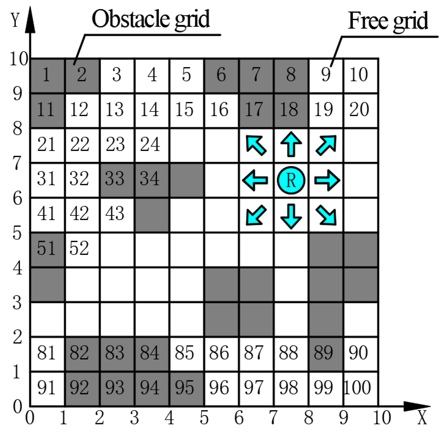
Due to its simplicity and efficiency, the grid-based approach is commonly employed for environment modeling [38]. Consequently, the environment is constructed by the grid method in this paper. In this representation, unoccupied grids are represented by 0 and displayed in white, whereas obstacle grids are marked by 1 and shown in black. To precisely identify the location of each grid cell, a Cartesian coordinate system, along with serial number notation, is utilized [39]. For example, Figure 1 presents an example of an environment modeled using the grid method. The modeled environment has 10 × 10 grids, where the robot “R” has eight optional grids available for movement during path planning.

In a Cartesian coordinate system, the center of each grid is uniquely determined by its absolute coordinates (x, y). Utilizing the serial numbering method, grid cells are sequentially assigned unique numbers from left to right and top to bottom starting from 1, ensuring that each cell is distinctly identified. The complete set of serial numbers assigned to all grids within the environment is expressed by the following (1):

$$\begin{array}{c}\hfill G=\left[1,2,3\dots g\right]g=m\times n.\end{array}$$

(1)

$$g=\left({\displaystyle \frac{x}{a}}+0.5\right)+n\times \left[m-\left({\displaystyle \frac{y}{a}}+0.5\right)\right].$$

(2)

$$x=\left\{\begin{array}{ll}\left[mod\right(g,n)-0.5]\times a,& if mod(g,n)\ne 0,\\ (n-0.5)\times a,& otherwise.\end{array}\right.$$

(3)

$$y=\left[m-ceil\left({\displaystyle \frac{g}{n}}\right)+0.5\right]\times a.$$

(4)

In Equations (1)–(4), g indicates the grid number; n and m denote the total number of rows and columns in the environment, respectively; and ${\delta }_x$ and ${\delta }_y$ refer to the mobile robot’s length and width, respectively. To ensure that the robot can perform in-place rotations and other maneuvers smoothly within free grid cells, the parameter a is set to the larger of ${\delta }_x$ and ${\delta }_y$. The $mod\left(\right)$ function calculates the remainder of a division operation, whereas the $ceil\left(\right)$ function rounds a given value up to the nearest integer.

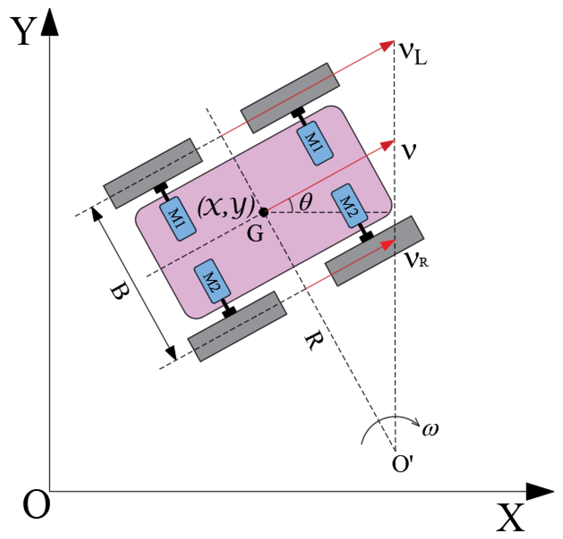
A differentially driven mobile robot (DDMR) is commonly utilized for validating path planning verification [40]. Figure 2 depicts the motion analysis of a DDMR during a turning maneuver, where linear velocities of the two driving wheels are expressed as follows:

$$\left\{\begin{array}{c}{v}_L=\left(R+B/2\right)\omega ,\\ v_R=\left(R-B/2\right)\omega ,\end{array}\right.$$

(5)

where $v_R$ and $v_L$ represent the inner and outer linear velocities of the DDMR, respectively; $G(x,y)$ signifies the location of the DDMR in the Cartesian coordinate framework; v denotes the linear velocity of the centroid; $\omega$ indicates the angular velocity of the DDMR as it turns around point $O^{\prime }$; the turning radius is R; and B signifies the width of the robot. As presented in Equation (5), the linear velocity of the centroid is formulated as follows:

$$v=\omega R=\left(v_R+v_L\right)/2.$$

(6)

It can be derived from Equations (5) and (6) that R and $\omega$ yield the following:

$$\left\{\begin{array}{c}\omega =B/\left(v_L-v_R\right),\\ R=\left[B\left(v_R+v_L\right)\right]/\left[2\left(v_L-v_R\right)\right].\end{array}\right.$$

(7)

According to Equation (7), when $v_L=-v_R$ and $R=0$, the DDMR achieves in-place rotation. During the turning process, if $\omega$ remains constant, the larger turning angle $\theta$, the more time it takes. This observation ensures that the DDMR can smoothly execute both turning and linear motion, providing the necessary conditions for verifying the paths calculated by the algorithm.

3. Brief Introduction of ACO

The ACO is employed to address optimization problems by imitating the natural foraging process of ants, which rely on pheromone trails to identify the shortest path from their nest to food sources. During the early phase of this process, ants explore their surroundings randomly. As they traverse different paths, they deposit pheromones along the path. The pheromone concentration increases as more ants follow a particular trail, reinforcing its attractiveness. This positive feedback loop encourages even more ants to choose the route with the strongest pheromone concentration, ultimately resulting in the identification of the shortest path.

Assuming that the kth ant moves from position i to position j at time t, where position i refers to the ant’s current grid and position j indicates the unvisited grid to which the ant will move. If there are multiple unvisited grids j around the current grid i, the transition probability $P_{ij}^k\left(t\right)$ is determined using Equation (8), and the grid j is selected using the roulette model. The following expression describes Equation (8):

$$P_{ij}^k\left(t\right)=\left\{\begin{array}{cc}{\displaystyle \frac{{\left[{\tau }_{ij}\left(t\right)\right]}^{\alpha }\ast {\left[{\eta }_{ij}\left(t\right)\right]}^{\beta }}{{\displaystyle \sum _{S\in A_k}}{\left[{\tau }_{is}\left(t\right)\right]}^{\alpha }\ast {\left[{\eta }_{is}\left(t\right)\right]}^{\beta }}},& ifj\in A_k,\hfill \\ 0,& otherwise,\hfill \end{array}\right.$$

(8)

where ${\tau }_{ij}\left(t\right)$ represents the pheromone amount between position i and position j at time t; $\alpha$ and $\beta$ refer to the pheromone concentration factor and expected heuristic factor, respectively; $A_k$ denotes the collection of unvisited grids around the position i; and ${\eta }_{ij}\left(t\right)$ indicates the heuristic value that can be determined by Equation (9):

$${\eta }_{ij}\left(t\right)={\displaystyle \frac{1}{d_{jg}}},$$

(9)

where $d_{jg}$ indicates the Euclidean distance between the next position j and the ending position. Once all ants have finished an iterative search, the pheromone on each path is updated using Equation (10):

$${\tau }_{ij}(t+1)=\left(1-\rho \right){\tau }_{ij}\left(t\right)+\sum _{k=1}^m\Delta {\tau }_{ij}^k,$$

(10)

where $\rho$ signifies of the pheromone evaporating rate parameter, $\Delta {\tau }_{ij}^k$ indicates the pheromone increment of kth ant from position i to position j in the current iterative cycle, and m denotes the total number of ants. The parameter $\Delta {\tau }_{ij}^k$ can be calculated as follows:

$$\Delta {\tau }_{ij}^k=\left\{\begin{array}{cc}{\displaystyle \frac{Q}{L_k}},& ifedge(i,j)ispassedbykthant,\hfill \\ 0,& otherwise,\hfill \end{array}\right.$$

(11)

where $L_k$ is the route length searched by the kth ant, while Q (the value remains fixed and positive) represents the pheromone accumulation parameter.

4. Introduction of EACI

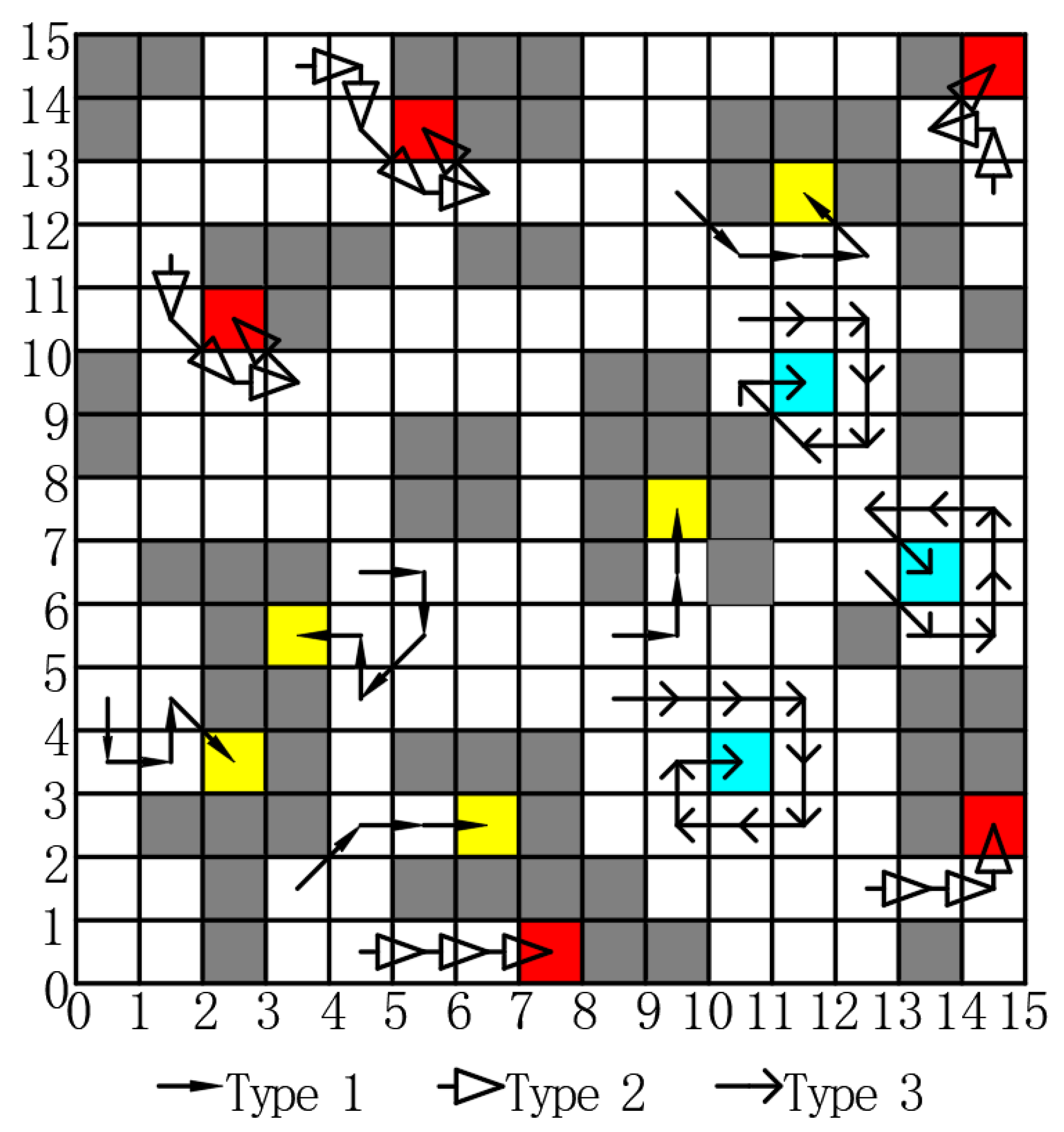
The conventional ACO has a disadvantage: it is prone to become trapped in local optimization early in the process. This issue arises because the selection of transition probability does not always guarantee the identification of the global optimal solution. In addition, the convergence rate is constrained by the limitations of a heuristic search. Consequently, higher environmental complexity increases the probability of stalemates for the ant. A significant challenge arises when the ants face restricted movement due to the presence of taboo lists, obstacles, and boundaries, leading to a condition called a deadlock. Specifically, the taboo list is a temporary memory maintained by each ant to store the nodes it has already visited during its current traversal, preventing it from revisiting the same nodes and forming cycles. Obstacles refer to impassable grid cells that represent physical barriers in the environment. Boundaries define the outer limits of the grid map, beyond which ants are not allowed to move. Hou et al. [41] categorized deadlock into three types, as illustrated in Figure 3. The first type of deadlock occurs when ants enter a dead end, which is indicated by a yellow grid. The second type of deadlock arises due to the combined influence of taboo lists, obstacles, and boundaries, which is denoted by a red grid. The third type of deadlock is exclusively caused by taboo lists, which is represented by a cyan grid.

For the purpose of enhancing the performance of ACO and to minimize the number of lost ants, we propose an enhanced variant algorithm of ACO—known as EACI. This algorithm incorporates several key modifications, including an island-based division strategy, a non-uniform pheromone distribution, an improved heuristic function, and an optimized global pheromone updating rule.

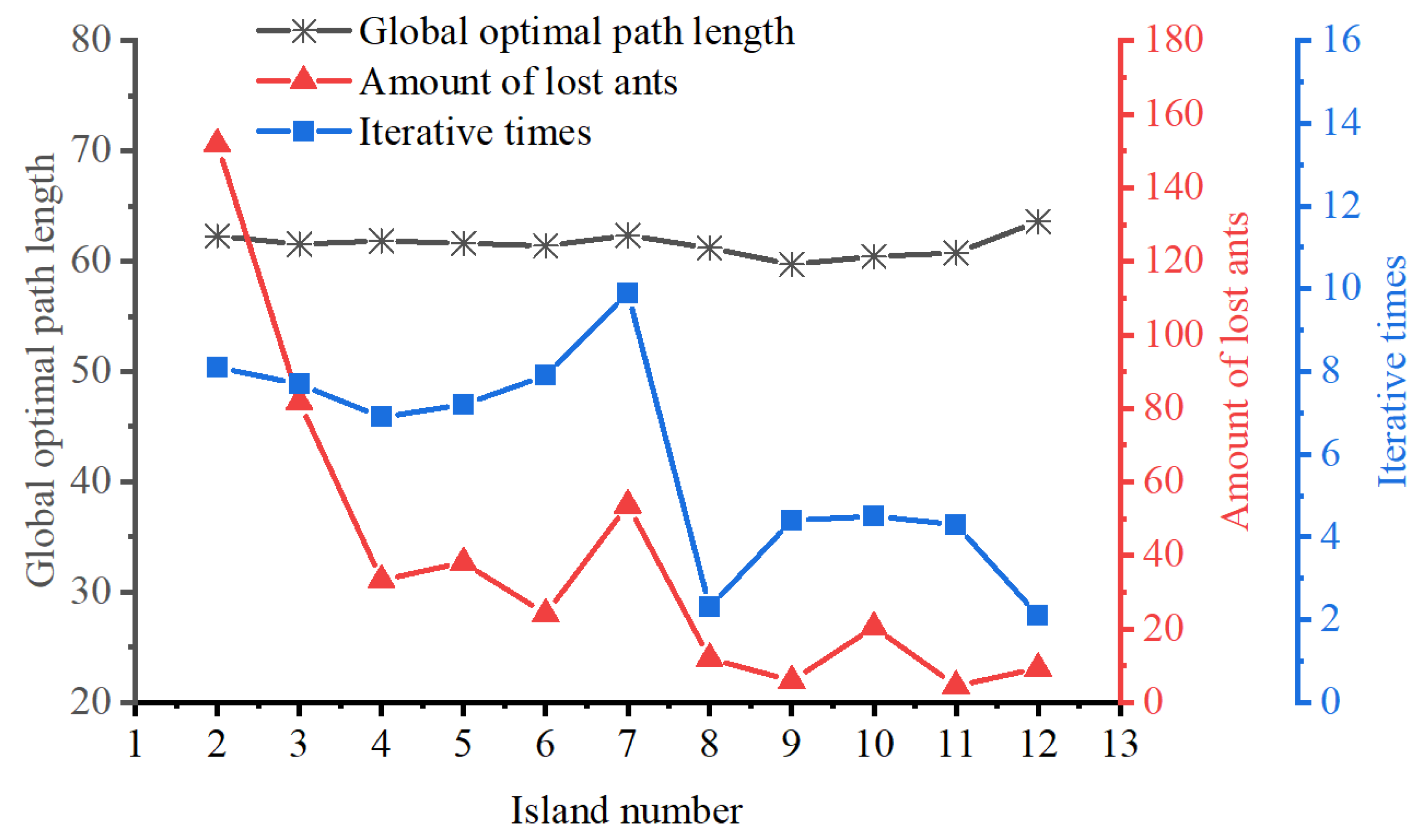
4.1. Island Division Strategy

To reducing the quantity of lost ants in a complex grid map, additional intermediate grids—referred to as “islands”—are introduced between the start (S) and end (E) points before path planning. These island grids represent mandatory waypoints that the optimal path must traverse. Consequently, the original environment map requires modification to ensure that the deadlock grid is not mistakenly selected as the island grid.

4.1.1. Grid Map Preprocessing

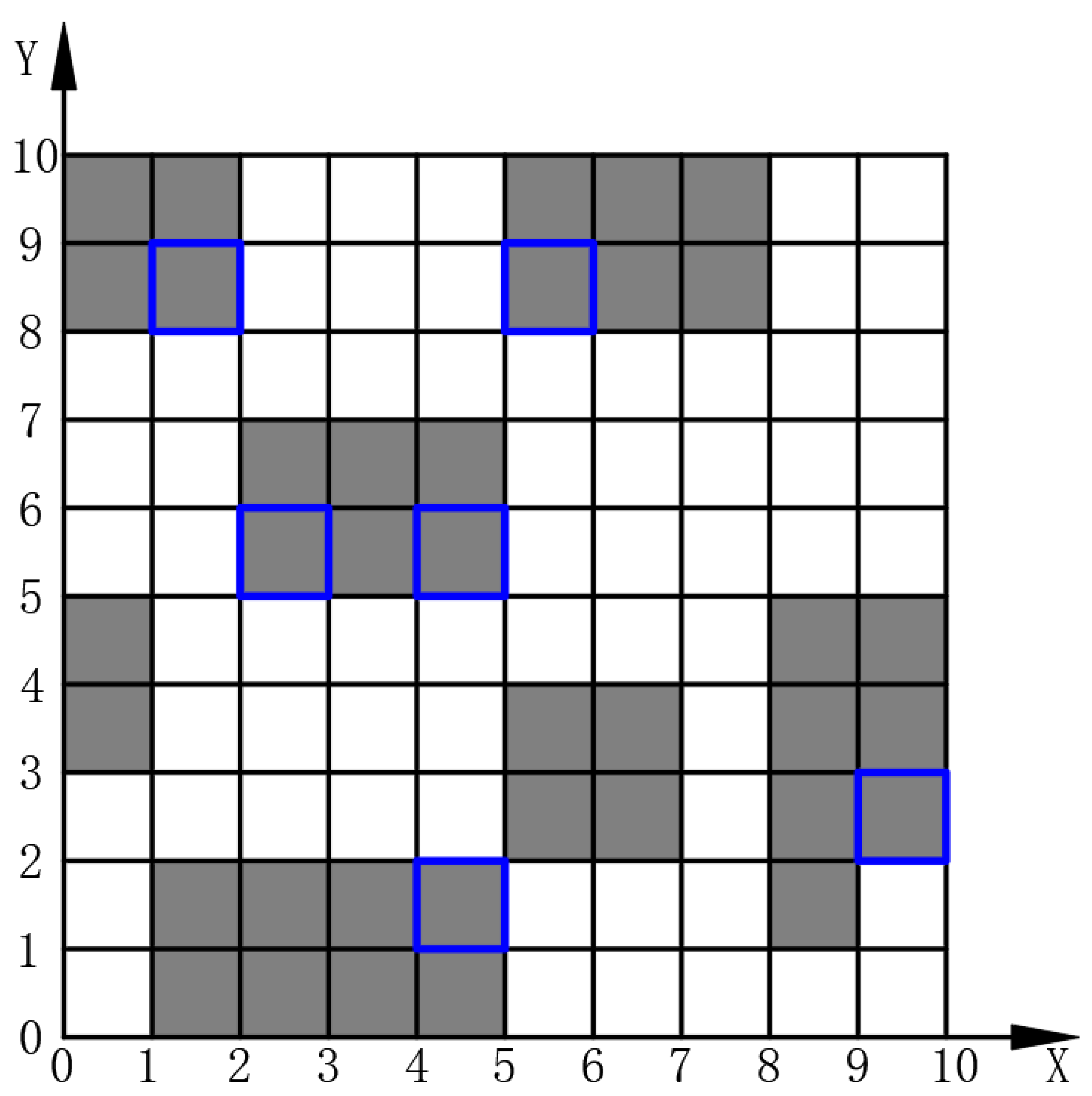
To prevent the selection of deadlock grids as island grids, it is essential to assess the status of the four adjacent grids surrounding each free grid. As illustrated in Figure 4, if two of these adjacent grids are classified as obstacle grids, the free grid is at risk of causing a deadlock. Consequently, it is transformed into an obstacle grid, represented by the number one, as specified in Equation (12). This preprocessing step converts the potential deadlock grids into obstacles, resulting in the creation known as the auxiliary map. For example, after preprocessing the grid map, as shown in Figure 1, the resulting auxiliary map, as depicted in Figure 5, highlights newly added obstacle grids, with black grids framed by blue borders.

$$G_{ij}=\left\{\begin{array}{cc}1,& if{G}_{i(j-1)}=1and{G}_{(i-1)j}=1,\hfill \\ 1,& otherwiseif{G}_{(i-1)j}=1and{G}_{i(j+1)}=1,\hfill \\ 1,& otherwiseif{G}_{i(j+1)}=1and{G}_{(i+1)j}=1,\hfill \\ 1,& otherwiseif{G}_{(i+1)j}=1and{G}_{i(j-1)}=1,\hfill \\ 0,& otherwise.\hfill \end{array}\right.$$

(12)

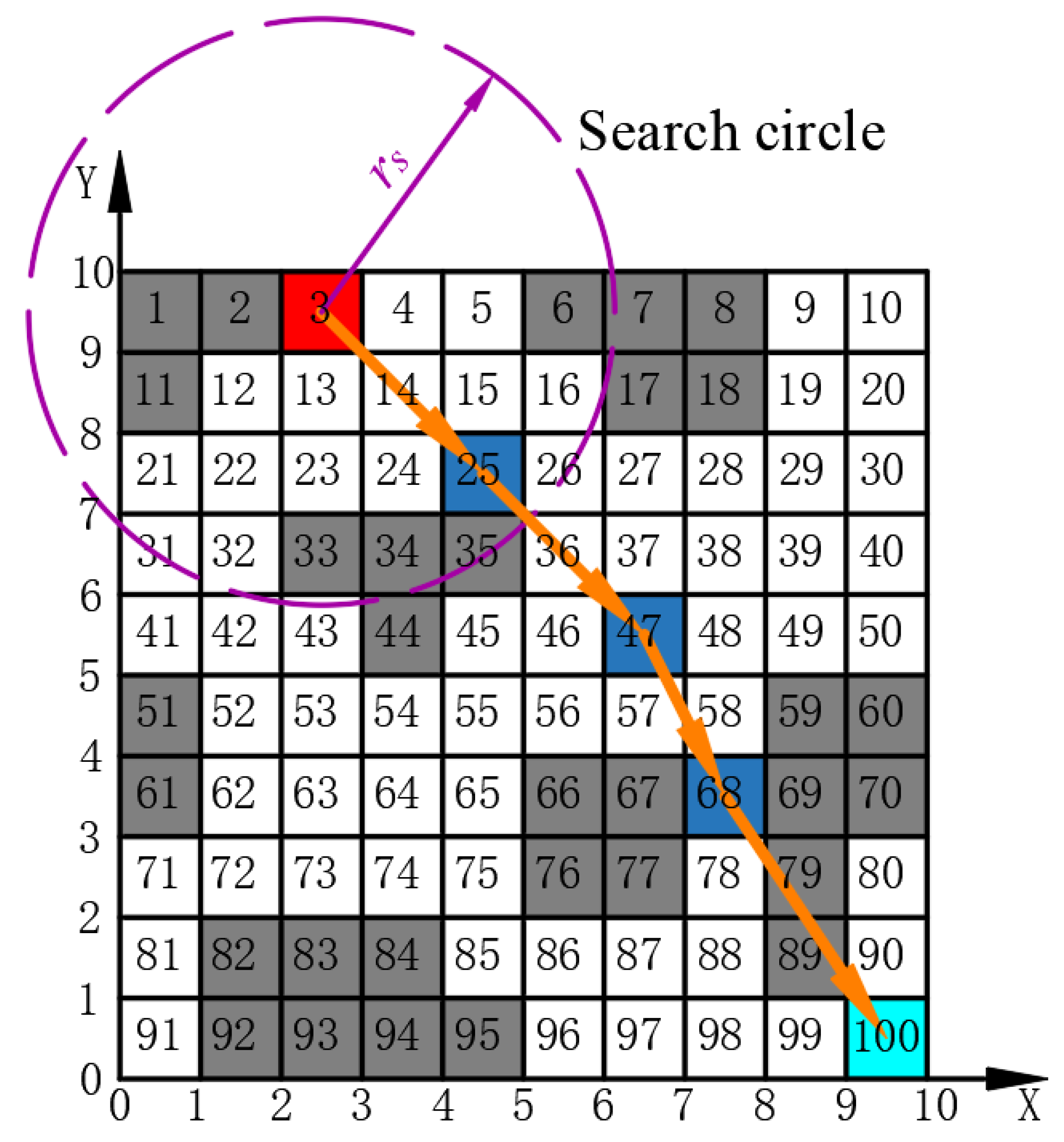
4.1.2. Islands Selection

To determine the location of the intermediate islands within the auxiliary map, it is essential to calculate the radius of the search circle ($r_s$). This radius can be expressed as follows:

$$r_s={\displaystyle \frac{d_{SE}}{N-1}},$$

(13)

where $d_{SE}$ signifies the Euclidean distance between S and E, and N refers to the total number of islands, including grids S and E. A search circle is defined with its center located at the grid corresponding to the starting grid S and a radius of $r_s$. The free grids within the search circle are designated as candidate grids. For each candidate grid, the sum of the Euclidean distances to both the starting and ending points is calculated independently. The detailed formula for this calculation is presented below:

$$D_I=\sqrt{{\left(x_I-x_S\right)}^2+{\left(y_I-y_S\right)}^2}+\sqrt{{\left(x_I-x_E\right)}^2+{\left(y_I-y_E\right)}^2}I\in A_I,$$

(14)

where $D_I$ indicates the sum of the Euclidean distances from the candidate grid, which is identified by the sequence number I to the starting point S $(S=L_1)$ and the endpoint E $(E=L_N)$, and $A_I$ signifies the set of sequence numbers for selectable grids. The candidate grid with the minimum $D_I$ value is selected, and its sequence number I is designated as the next island $L_2$. Taking the grid center of $L_2$ as the reference point, the above steps are repeated until the search circle includes the endpoint E $(E=L_N)$, thereby determining the sequence of all islands as follows:

$$L_{order}=\left[L_1,L_2\cdots ,L_z,\cdots L_N\right],$$

(15)

where $L_z$ indicates the serial number of the zth island.

Taking the auxiliary map of Figure 1 as an example, as shown in Figure 6, 3 and 100 represent the starting position and target position, respectively. Assuming that the map requires five islands, the final path planning sequence is given by $I_{order}=\left[3,25,47,68,100\right]$. The EACI algorithm sequentially generates the local optimal path between the two adjacent sequence numbers. Connecting all local optimal paths from start to end yields the global optimal path for the entire complex map.

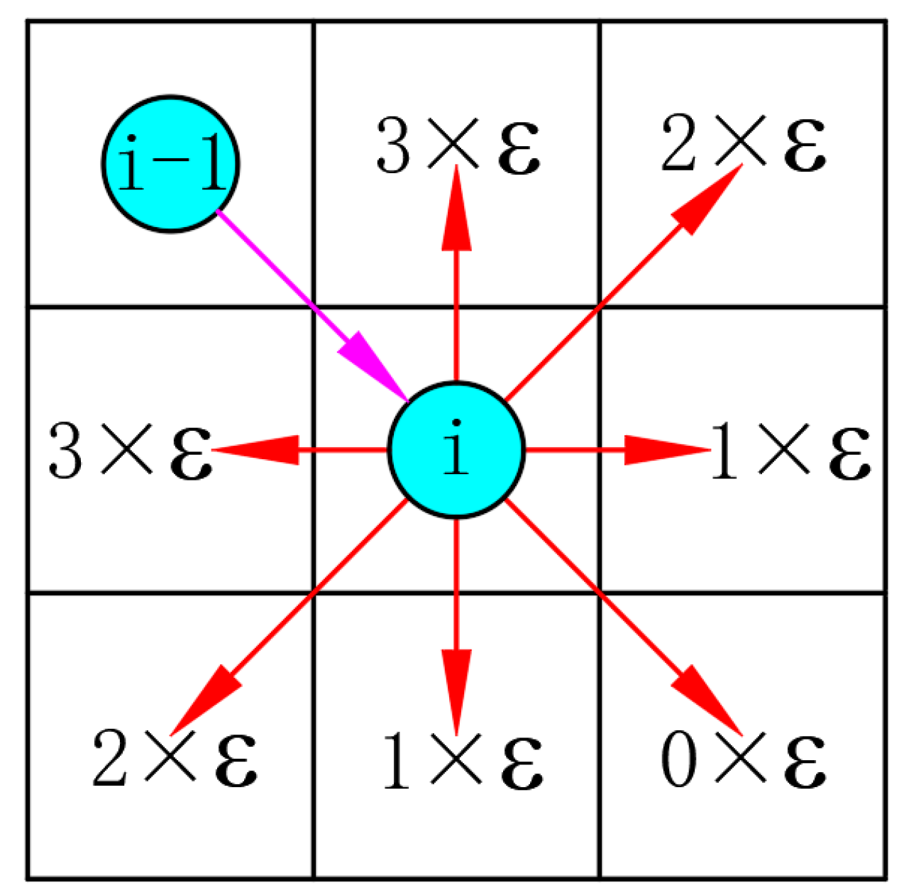
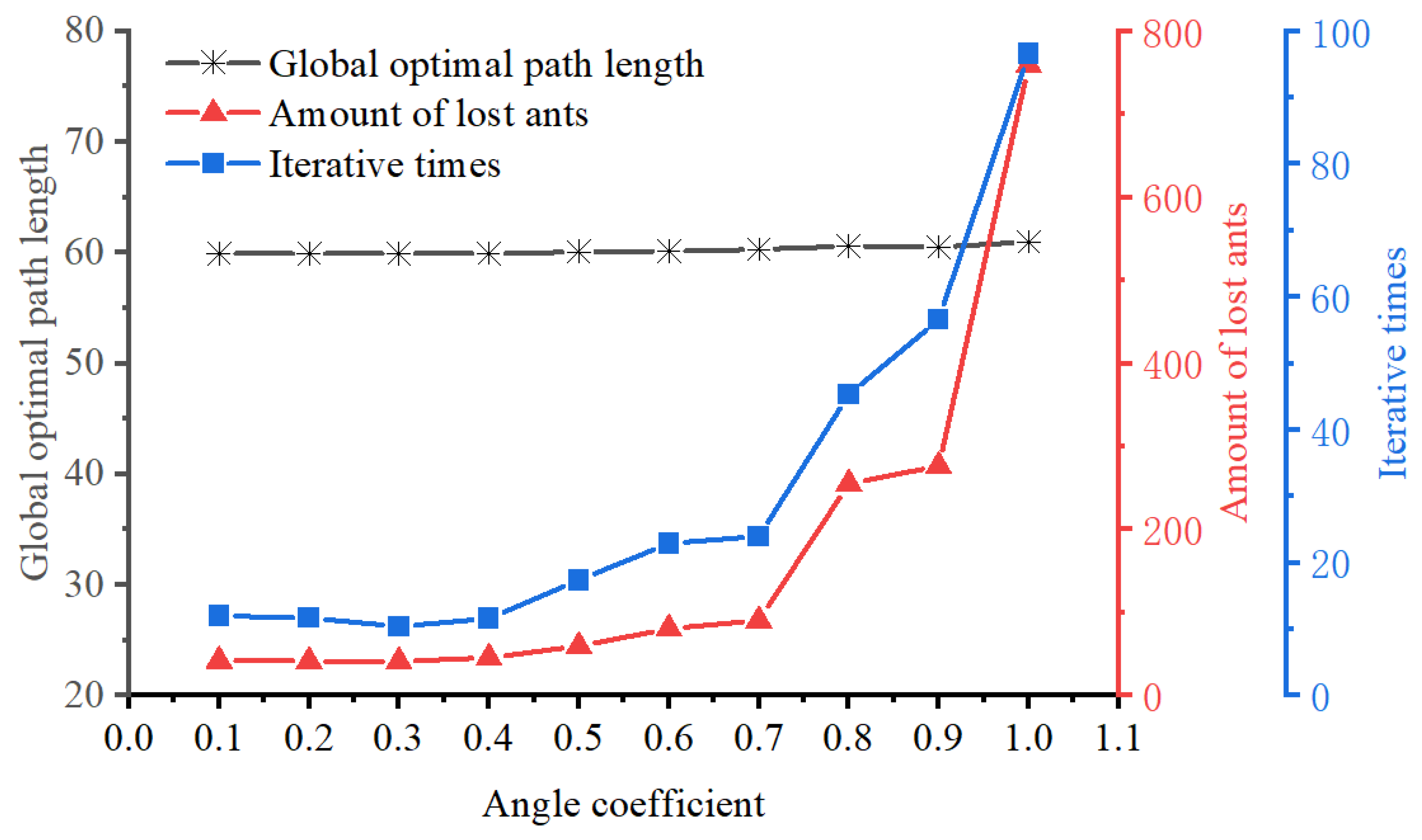
4.2. Modified Heuristic Function

In the basic ACO, the heuristic value only considers the distance between each free grid and the target grid, neglecting the impact of the turning angle in the optimal path calculation. However, a larger turning angle results in higher energy consumption. To address this issue, this study modifies the heuristic function by incorporating the turning angle variable. The specific calculation is shown in Equation (16):

$${\eta }_{ij}={\displaystyle \frac{1}{d_{jg}+{\sigma }_{ij}}},$$

(16)

where $d_{jg}$ signifies the distance between the next position j and the ending position, and ${\sigma }_{ij}$ indicates the angle coefficient. The distribution of angle coefficients from node i to node j is illustrated in Figure 7 and can be calculated using Equation (17):

$${\sigma }_{ij}=\left\{\begin{array}{cc}0\times \epsilon ,& if<\overrightarrow{P_{i-1}{P}_i},\overrightarrow{P_i{P}_j}>=0,\hfill \\ 1\times \epsilon ,& otherwiseif<\overrightarrow{P_{i-1}{P}_i},\overrightarrow{P_i{P}_j}>={\displaystyle \frac{\pi }{4}},\hfill \\ 2\times \epsilon ,& otherwiseif<\overrightarrow{P_{i-1}{P}_i},\overrightarrow{P_i{P}_j}>={\displaystyle \frac{\pi }{2}},\hfill \\ 3\times \epsilon ,& otherwiseif<\overrightarrow{P_{i-1}{P}_i},\overrightarrow{P_i{P}_j}>={\displaystyle \frac{3\pi }{4}},\hfill \end{array}\right.$$

(17)

where $\epsilon$ signifies the angle coefficient; $\overrightarrow{P_{i-1}{P}_i}$ refers to the vector that starts with node $i-1$ and ends with node i; node $i-1$ denotes the previous node of node i in the path; node i implies the current position of the robot; $\overrightarrow{P_i{P}_j}$ refers to the vector that starts with node i and ends with node j; node j indicates the next node of node i in the path; node j represents the node to be selected by the robot in the path planning; and $<\overrightarrow{P_{i-1}{P}_i},\overrightarrow{P_i{P}_j}>$ refers to the angle between vector $\overrightarrow{P_{i-1}{P}_i}$ and vector $\overrightarrow{P_i{P}_j}$.

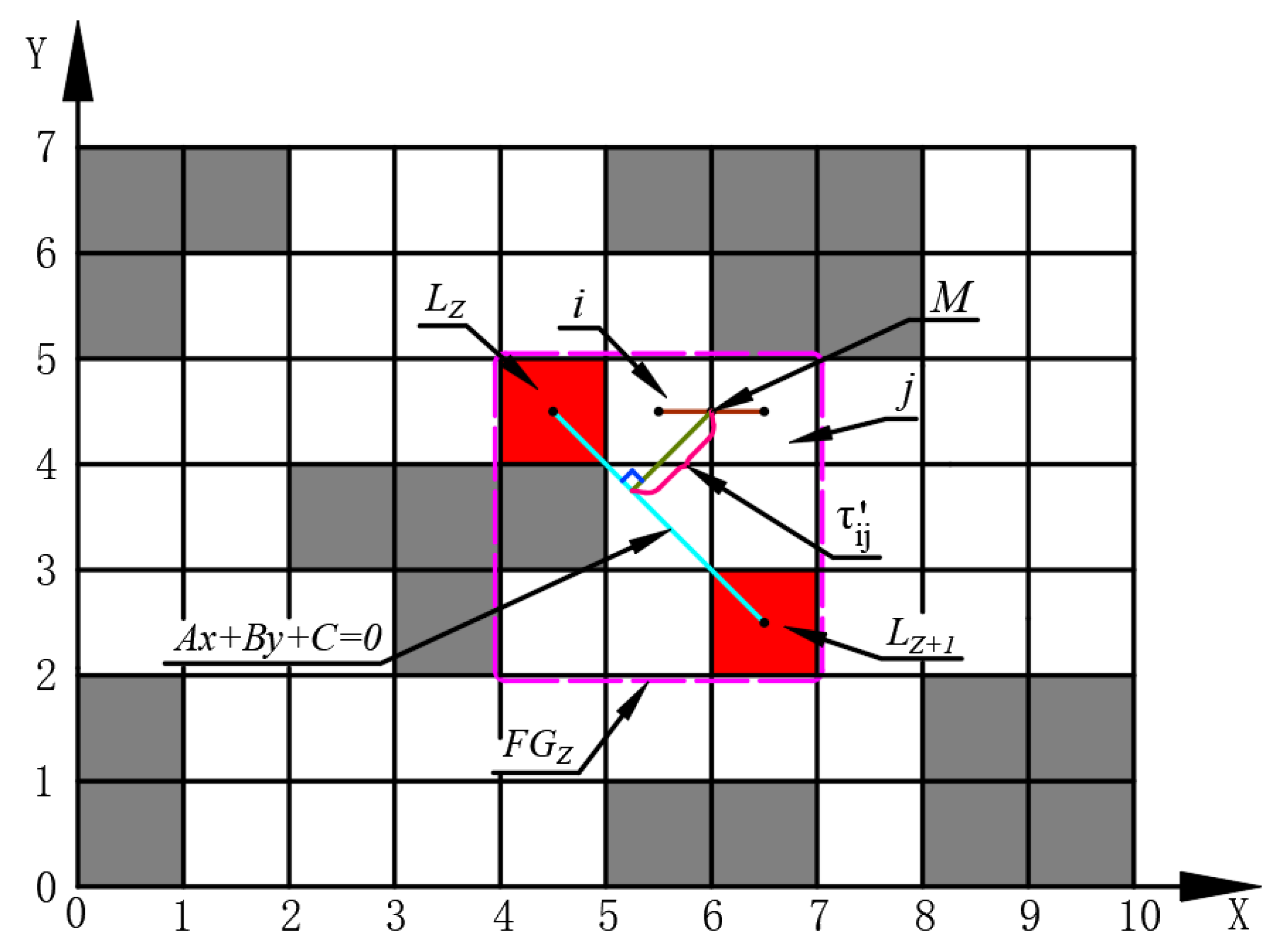
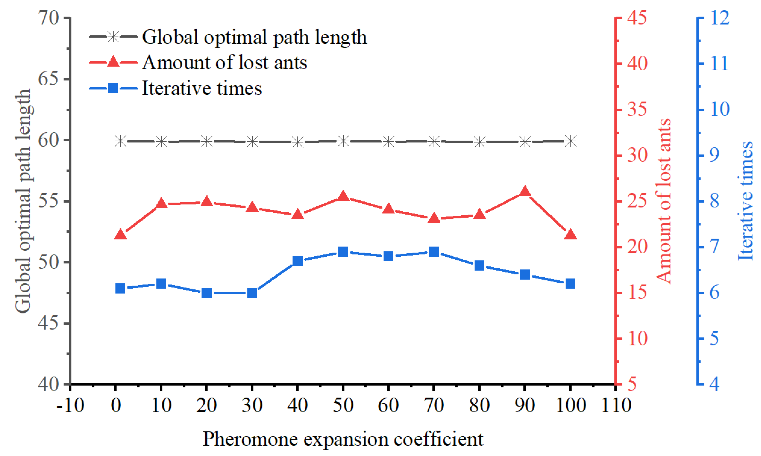
4.3. Improved Distribution of the Initial Pheromones

During the initial phase of ACO, the pheromone values are uniformly distributed throughout the environment. As a result, ants explore paths with a certain degree of randomness, leading to slow algorithm convergence. To address this issue, this article introduces an uneven initial pheromone distribution strategy, with its calculation principle illustrated in Figure 8.

The rectangular region (with the adjacent island number $L_z$ and $L_{z+1}$ as vertices) is designated as the favorable region $F{G}_z$. The equation of the straight line passing through points $L_z$ and $L_{z+1}$ is determined based on their coordinates:

$$Ax+By+C=0,$$

(18)

where A, B, and C refer to the relevant parameters of the linear equation.

The formula for calculating the midpoint coordinate $M(x_M,y_M)$ of the adjacent path nodes $i(x_i,y_i)$ and $j(x_j,y_j)$ within the rectangular area $F{G}_z$ is expressed in Equation (19). The local initialization pheromone concentration for this region is calculated by Equation (20). Subsequently, the local initialization pheromone concentration of other favorable regions in the environment is calculated in sequence. Finally, the non-uniform initial pheromone distribution for the entire map can be calculated using Equation (21):

$$\left\{\begin{array}{c}{x}_M={\displaystyle \frac{x_i+x_j}{2}},\hfill \\ y_M={\displaystyle \frac{y_i+y_j}{2}}.\hfill \end{array}\right.$$

(19)

$${\tau }_{ij}^{\prime }=\left\{\begin{array}{cc}{\displaystyle \frac{\sqrt{A^2+B^2}}{\left|A{x}_M+B{y}_M+C\right|}},\hfill & ifi,j\in F{G}_z,i\ne j,A{x}_M+B{y}_M+C\ne 0,\hfill \\ +\infty ,\hfill & otherwiseifi,j\in F{G}_z,i=j,A{x}_M+B{y}_M+C=0,\hfill \\ {\displaystyle \frac{\sqrt{A^2+B^2}}{\left|A{x}_i+B{y}_i+C\right|}},\hfill & otherwiseifi,j\in F{G}_z,i\ne j,A{x}_M+B{y}_M+C=0.\hfill \end{array}\right.$$

(20)

$${\tau }_{ij}\left(0\right)=\left\{\begin{array}{cc}{\tau }_{ij}^{\prime },\hfill & ifi,j\in F{G}_{z}and{\tau }_{ij}^{\prime }\ne +\infty ,\hfill \\ \lambda \ast \max {\tau }_0,\hfill & otherwiseifi,j\in F{G}_{z}and{\tau }_{ij}^{\prime }=+\infty ,\hfill \\ \min {\tau }_0,\hfill & otherwiseifi,j\in F{G}_z,\hfill \end{array}\right.$$

(21)

where ${\tau }_{ij}^{\prime }$ indicates the local initialization pheromone concentration from node i to node j in the rectangular area $F{G}_z$; ${\tau }_{ij}\left(0\right)$ refers to the global pheromone concentration from node i to node j in any region of entire map; $FG$ implies the grid set of all favorable region; $\lambda$ represents the pheromone expansion coefficient; and $\max {\tau }_0$ and $\min {\tau }_0$ signify the maximum and minimum values of pheromone concentration in all favorable region, respectively. The latter can be expressed as follows:

$$\left\{\begin{array}{cc}\max {\tau }_0=\arg \max \left({\tau }_{ij}^{\prime }\right),\hfill & ifi,j\in FGand{\tau }_{ij}^{\prime }\ne +\infty ,\hfill \\ \min {\tau }_0=\arg \min \left({\tau }_{ij}^{\prime }\right),\hfill & otherwiseifi,j\in FG.\hfill \end{array}\right.$$

(22)

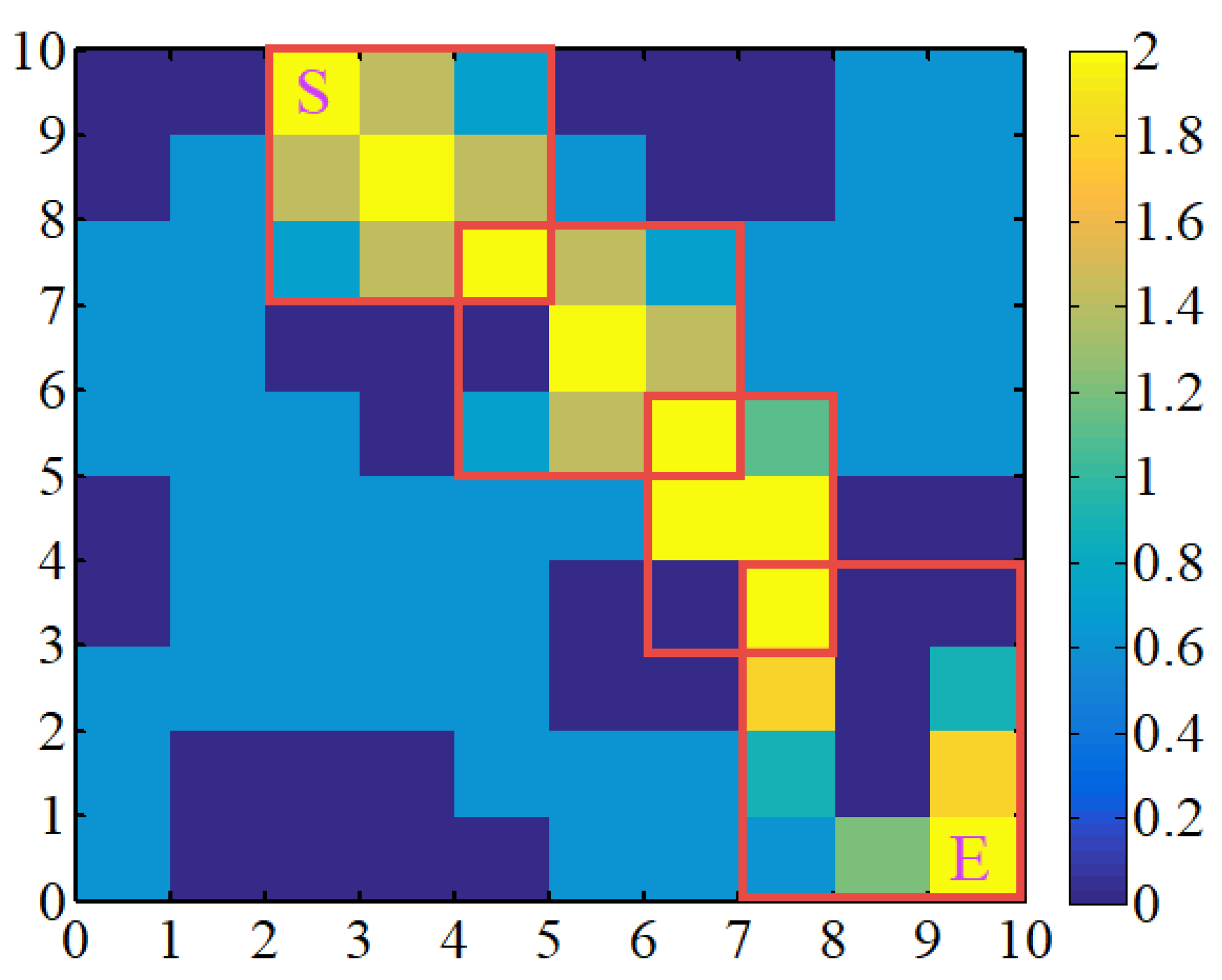
A case of an uneven initial pheromone distribution is shown in Figure 9, where each red rectangle represents a favorable area between adjacent islands.

4.4. Adaptive Pheromone Update Rule

Once all ants finish an iterative cycle, the pheromones on the original path volatilize at a certain speed, while the new pheromones are deposited by ants traversing through the path. After multiple iterations, the optimal route is identified as the one with highest pheromone concentration. In this study, an improved pheromone update rule is introduced to accelerate pheromone accumulation speed on the optimal route, reduce the pheromone accumulation rate on the worst route, and incorporate a dynamic adaptive volatilization coefficient. The specific calculations are presented as follows:

$${\tau }_{ij}(t+1)=(1-\rho ){\tau }_{ij}\left(t\right)+\sum _{k=1}^m{\Delta }_{ij}^k+\rho \Delta {\tau }_{ij}^{\ast }.$$

(23)

$$\Delta {\tau }_{ij}^{*}=\left\{\begin{array}{cc}{\displaystyle \frac{\kappa \ast Q\ast d_{SE}}{L_{best}^2}},\hfill & ifedge(i,j)belongstotheoptimumpath,\hfill \\ -{\displaystyle \frac{\kappa \ast Q\ast d_{SE}}{L_{worst}\ast L_{best}}},\hfill & otherwiseifedge(i,j)belongstotheworstpath,\hfill \\ 0,\hfill & otherwise.\hfill \end{array}\right.$$

(24)

$$\rho =\kappa \ast \left({\displaystyle \frac{d_{SE}}{L_{best}}}\right).$$

(25)

When all ants complete an iteration, the pheromones of the entire map will be updated by Equation (23), where $(1-\rho ){\tau }_{ij}\left(t\right)$ represents the volatilization term, indicating the volatilization of the original pheromone; ${\sum }_{k=1}^m{\Delta }_{ij}^k$ implies the item of pheromones addition, signifying the addition of new pheromones to the path the ants have passed; and $\Delta {\tau }_{ij}^{*}$ refers to the term of reward or punishment, which can be calculated according to Equation (24). This observation involves enhancing the optimal path by adding extra pheromones to reinforce its guidance for subsequent iterations while reducing pheromones on the worst path to minimize its misleading effect. $L_{best}$ represents the optimum route length; $L_{worst}$ implies the worst route length in current iteration; and $\rho$ denotes the adaptive volatilization rate, which can be calculated using Equation (25), where $\kappa$ implies the adjustment coefficient ranging from 0 to 1. From this formula, we can conclude that, at the beginning of the algorithm, a large $L_{best}$ leads to a small $\rho$ and minimal differences in the pheromone values across paths, allowing the ant colony to maintain a strong global path planning capability. As $L_{best}$ decreases, the value of $\rho$ increases gradually, leading to greater differences in pheromone values across paths. Consequently, more ants are guided toward the optimal path, allowing the algorithm to achieve faster convergence in later stages.

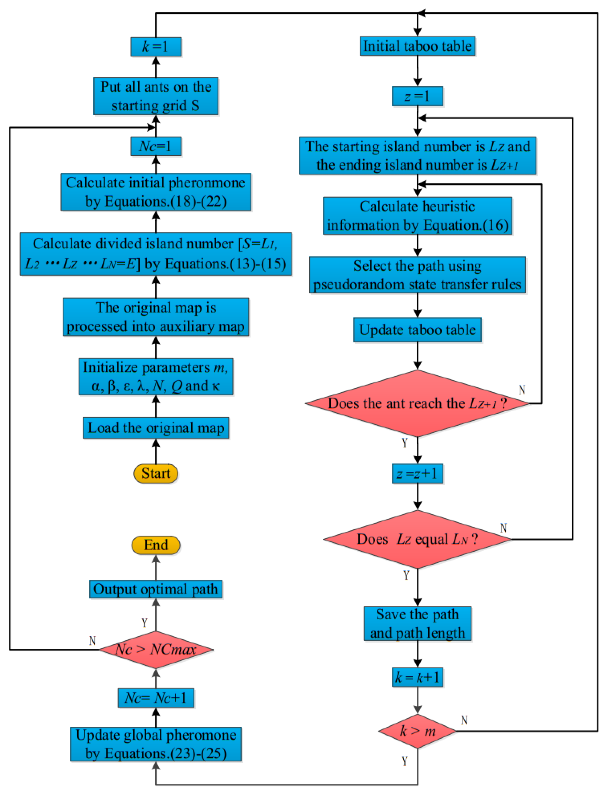
5. Process of EACI for Path Planning

In order to improve ACO efficiency, reduce turning angles, and minimize deadlock ants, this study introduces the EACI algorithm. The steps for applying EACI in path planning are outlined below.

Step 1 Initialize the parameters: The parameters, including S, E, m, $\alpha$, $\beta$, $\epsilon$, $\lambda$, N, Q, and $\kappa$, are initialized. Simultaneously, the maximum and current iterations are set to $N{c}_{max}$ and $Nc$.

Step 2 Determine the divided island number based on Equations (13)–(15).

Step 3 Calculate ${\tau }_{ij}\left(0\right)$, which indicates the initial pheromone, and it is calculated according to Equations (18)–(22).

Step 4 Path selection: First, the beginning position S is designated as the first island, while the ending point E is set as the Nth island. The sequence of all islands can be represented as $\left[S=L_1,L_2\cdots ,L_z,\cdots L_N=E\right]$. Additionally, the number of deadlock ants is initialized to 0. In addition, the ant is initially placed on the first island. Using Equations (8), (16), and (17), the next grid j is calculated. Once the ant passes through the grid j, it is added to the taboo list, and this process is repeated. If the ant successfully reaches the next island, that island becomes the new starting position, and the path planning continues, passing through the intermediate islands in sequence until the target point is reached. The complete path formed by connecting all the nodes—which the ant has passed through—is the path discovered by the ant. If the ant has a deadlock between any two adjacent islands, it halts its route search, and the number of lost ants increases by 1. Finally, another ant is placed at the first island to begin path planning from grids S to E, following the same process as the previous ant. The iterative cycle continues until all ants have completed their path planning.

Step 5 Global update of the pheromones: Once an iterative search is completed, the paths searched by all ants, from S to E, are recorded. The longest and the shortest path lengths are identified from these records. The adaptive volatilization coefficient $\rho$ can then be calculated using Equation (25). Following this, the pheromones on shortest route are rewarded, and the pheromones on the longest route are punished, as described in Equation (24). Finally, the global pheromones for the whole map are updated according to Equation (23).

Step 6 Search end: If $Nc$ exceeds $N{c}_{max}$, the outputs include the optimal route length, its sequence, deadlock ant count, and other associated parameters. Otherwise, let $Nc=Nc+1$ and clear the taboo list. Then, return to Step 4 and continue the path planning process until the stopping condition appears.

Step 7 Output the optimal solution.

The flowchart demonstrating the EACI algorithm for path planning is shown in Figure 10.

6. Simulation and Analysis

6.1. Determination of Parameter Optimization Combination

In this study, to determine the optimal combination of parameters, numerous simulation experiments were conducted using both empirical and experimental methods [30]. The experiments were conducted on a laptop equipped with a 12th Gen Intel^® Core™ i7-12700H processor (2.30 GHz) and 16 GB of RAM using MATLAB R2021b as the simulation platform.

A group of parameters was established for the simulation experiments, where, in each experiment, only one of the parameters was varied, while the others remained constant. Each experiment was run ten times with the same parameters to minimize the impact of random variations, and the average of all the results was calculated. The advantages and disadvantages of different parameter combinations were analyzed, including the number of iterations, the length of the global optimal route, and the quantity of deadlock ants encountered during the algorithm’s execution. Since parameters $\alpha$ and $\beta$ have been extensively studied, this study primarily focuses on optimizing parameters $\epsilon$, $\lambda$, $\kappa$, and N.

In a certain map, the parameters are set as follows: $m=50$, $N{c}_{max}=100$, $\alpha =1.1$, $\beta =7$, $Q=100$, $\kappa =0.9$, $N=6$, and $\lambda =3$. The number of iterations, global optimal route length, and the amount of deadlock ants are monitored for each set of parameters, including $\epsilon =0.1$, $\epsilon =0.2$, $\epsilon =0.3$, ⋯, and $\epsilon =1.0$. The detailed simulation results of the EACI are shown in Figure 11.

From Figure 11, as the angle coefficient increases, the optimal path length changes very slightly, but both the number of lost ants and iterations increase gradually. When the parameters are set to $\epsilon \in [0.1,0.7]$, the EACI algorithm demonstrates good performance in all the three aspects mentioned above.

Under the condition of the same grid map, the setting parameters are as follows: $m=50$, $N{c}_{max}=100$, $\alpha =1.1$, $\beta =7$, $Q=100$, $\kappa =0.9$, $N=6$, and $\epsilon =0.5$. When the parameters were varied as $\lambda =1$, $\lambda =10$, $\lambda =20$, ⋯, and $\lambda =100$, the experimental simulation results of the EACI were recorded, as presented in Figure 12.

By analyzing Figure 12, it can be observed that, regardless of the pheromone expansion coefficient $\lambda$, the EACI algorithm showed minimal variations in the optimal route, iterative times, and the quantity of deadlock ants. This observation suggests that $\lambda$ does not significantly affect the path planning performance of the EACI algorithm.

In the same environment, experiments were conducted with the varying parameters $N=2$, $N=3$, ⋯, and $N=12$, while the remaining parameters were set as $m=50$, $N{c}_{max}=100$, $\alpha =1.1$, $\beta =7$, $Q=100$, $\kappa =0.9$, $\lambda =3$, and $\epsilon =0.5$. The simulation results were plotted as a curve, as presented in Figure 13.

By analyzing Figure 13, it is clear that the optimal route path length remains relatively stable as the number of islands increases, while iterative times and deadlock ants gradually decrease, with iterative times fluctuating between 1 and 10. Additionally, the figure shows that adding more islands does not necessarily improve performance; beyond a certain point, the algorithm’s efficiency no longer improves. In this experiment, the EACI demonstrated good performance when $N\in [6,12]$.

The parameters for the same environment were set as follows: $m=50$, $N{c}_{max}=100$, $\alpha =1.1$, $\beta =7$, $Q=100$, $\lambda =3$, $N=12$ $\epsilon =0.5$, $\kappa =0.3$, $\kappa =0.4$, ⋯, and $\kappa =1.3$. The results of the experiment are presented in Figure 14.

An analysis of Figure 14 reveals that the influence of the adaptive coefficient $\kappa$ on the experimental outcomes closely resembles the effect of varying the number of islands. Regardless of the specific value of $\kappa$, the EACI algorithm consistently identifies the optimal path length. However, as $\kappa$ increases, there is a noticeable decline in both the number of iterations required and the number of ants lost during the process. When, the reduction in lost ants slows down, the number of iterations initially increases slightly and then, subsequently, decreases. Overall, when $\kappa \in [0.9,1.3]$, the EACI algorithm demonstrates strong performance across all evaluated criteria.

6.2. Comparison with Other Algorithms

To verify the effectiveness of the proposed algorithm, a specific grid map was selected as the simulation environment, and it was consistent with the experimental setups described in the literature [29,41]: Luo et al. [29] proposed the improved ant colony optimization algorithm (IACO), and Hou et al. [41] proposed an enhanced ant colony algorithm with a communication mechanism (CMEACO). To ensure a comprehensive performance evaluation, the standards ACO, IACO, and CMEACO were compared with the proposed EACI algorithm. For the sake of comparison, the same grid map was also selected as the test environment for simulation experiments, The initialization parameters were configured as follows: $m=50$, $N{c}_{max}=100$, $\alpha =1.1$, $\beta =7$, $Q=100$, $\kappa =0.9$, $\lambda =3$, $N=9$, and $\epsilon =0.5$.

6.2.1. Environment with 20 × 20 Grids

In a simple environment, the start and end positions are assigned sequence numbers 1 and 400, respectively. The initial pheromone distribution of EACI is illustrated in Figure 15, while Figure 16 presents the pheromone distribution across different iterations.

To ensure a more objective evaluation of the algorithm and to minimize the impact of random factors, each simulation experiment was conducted 20 times. The comparative simulation results of the four algorithms—ACO, IACO, CMEACO, and EACI—are illustrated in Figure 17, where each algorithm generated an optimal path. Figure 18 presents the convergence curves of the optimal paths for the four algorithms, while Figure 19 depicts the number of lost ants produced by each algorithm. Furthermore, the average values of relevant parameters were calculated, with the detailed statistical results summarized in

Table 1. Summary of the relevant data generated by the four simulation algorithms in the 20 × 20 grid environment.

Item	Average Iterative Times	Average of Path Length	Optimal Route Length	Standard Deviation	Mean Value of Lost Ants	Total Corner Angle (°)
ACO	40.5	30.97	30.97	0	1246.0	675
IACO	10.5	30.97	30.97	-	172.3	675
CMEACO	6.4	30.97	30.97	0	165.10	585
EACI	1	30.97	30.97	0	9.85	675

.

As presented in Figure 15 and Figure 16, it is obvious that the pheromone quickly concentrates on the optimal path as the number of iterative times grows. As illustrated in Figure 16a, a large amount of pheromones was distributed near the optimal path after the first iteration, clearly indicating that EACI is capable of identifying the optimal route from the very beginning. Figure 16b depicts that, after the fifth iteration, the pheromones were entirely concentrated on the optimal path, with only minimal changes in subsequent iterations, thereby validating the extremely fast convergence speed of EACI.

As presented in Figure 17, all four algorithms successfully captured the path from the starting to the ending points. The convergence curves of the optimal path for these algorithms are shown in Figure 18, while Table 1 provides a summary of the experimental results. Among the four algorithms, EACI demonstrated the fastest convergence speed. However, its total turning angle was 675°, which was identical to that of the ACO and IACO but slightly larger than CMEACO. As depicted in Figure 19, as the number of iterations increased, the occurrence of deadlock ants decreased for all algorithms. Notably, EACI produced the fewest deadlock ants and exhibited the most rapid decline in their numbers, further highlighting its efficiency in path optimization. Table 1 shows that all algorithms successfully identified the shortest path, with a length of 30.97. The most notable observation was that EACI resulted in the least average number of deadlock ants and the lowest average number of iterations among the four algorithms, with values of 9.85 (9.85 < 165.10 < 172.3 < 1246.0) and 1 (1 < 6.4 < 10.5 < 40.5), respectively, which are provided in the table. Overall, the experiments confirmed that EACI has excellent performance.

6.2.2. Environment with 30 × 30 Grids

In the complex environment, the start and end positions were assigned sequence numbers 871 and 30, respectively. The initial pheromone distribution of the EACI is depicted in Figure 20, while Figure 21 shows the pheromone distribution across the different iterations. To ensure a more objective evaluation and to minimize the impact of random factors, each simulation experiment was repeated 20 times. The simulation results of the four algorithms—ACO, IACO, CMEACO, and EACI—are shown in Figure 22, where each algorithm generates an optimal path. The convergence curves of the optimal paths for these algorithms are presented in Figure 23, while Figure 24 illustrates the number of lost ants produced by each algorithm. Additionally, the average values of the relevant parameters were calculated, with the detailed statistical results provided in

Table 2. Summary of the relevant data generated by the four simulation algorithms in the 30 × 30 grid environment.

Item	Average Iterative Times	Average of Path Length	Optimal Route Length	Standard Deviation	Mean Value of Lost Ants	Total Corner Angle (°)
ACO	77.10	45.89	45.36	1.6564	3112.40	675
IACO	21.90	45.22	44.53	0.5409	415.30	810
CMEACO	11.7	44.70	44.53	0.2043	237.70	630
EACI	1.4	44.53	44.53	0	27.5	765

.

As shown in Figure 20 and Figure 21, the pheromone aggregation speed of the EACI algorithm was slower in a complex map than in a simple map. Figure 21a,b indicate that, within five iterations, a significant amount of pheromones has already accumulated near the optimal path. Figure 21c shows that, within 15 iterations, the pheromones have completely concentrated on the optimal path. The results in Figure 23 indicate that the EACI algorithm achieved optimal route detection as early as the second iteration, showcasing its efficient convergence.

As depicted in Figure 22, all four algorithms successfully identified a path from the starting points to the endpoints. The comparison in Figure 23 illustrates that EACI outperformed the other algorithms by producing the shortest path and converging at the fastest rate. Furthermore, Figure 24 illustrates that, as the iterative times increased, the occurrence of deadlock ants gradually decreased for all algorithms. Notably, EACI generated the fewest deadlock ants and exhibited the most rapid decline in their numbers. As presented in Table 2, the shortest path length generated by EACI was 44.53, which aligns with the results of IACO and CMEACO, but it was 0.83 shorter than that of ACO. Moreover, the average path length produced by EACI was also 44.53, which is comparable to that of CMEACO; however, it was 0.69 and 1.36 shorter than those of IACO and ACO, respectively. The two parameters that showed the most significant changes, as shown in Table 2, were the average iterations and the mean number of lost ants. The average iterative times calculated by IEAC was 1.4, which was approximately 1/11 of CMEACO, 1/21 of IACO, and 1/77 of ACO. Regarding the average number of lost ants, EACI produced a value of 27.5, which was 210.2 fewer than CMEACO, 384.3 fewer than IACO, and 3084.9 fewer than ACO. The total turning angle of the route was 765°, which was slightly higher than those of CMEACO and ACO but lower than that of IACO. This observation suggests that there is still potential for improvement in optimizing the total turning angle within the EACI algorithm. Overall, the data above clearly demonstrate that EACI exhibited outstanding performance.

6.2.3. Environment with 40 × 40 Grids and 50 × 50 Grids

To further verify the performance of the proposed algorithm in more complex environments, two additional experimental scenarios were selected: 40 × 40 and 50 × 50 grid environments. In these scenarios, the start positions were assigned sequence numbers 1 and 2451, and the goal positions were 1600 and 50, respectively. To ensure the objectivity of the evaluation and to minimize the influence of random factors, each simulation experiment was repeated 20 times. Four algorithms—ACO, IACO, MAACO (Modified Adaptive Ant Colony Optimization Algorithm) [42], and EACI—were compared in terms of optimal path, convergence curve, and number of lost ants. In the 40 × 40 grid environment, the optimal paths generated by each algorithm are shown in Figure 25, the convergence curves of the optimal paths are presented in Figure 26, and the number of lost ants for each algorithm is illustrated in Figure 27. In the 50 × 50 grid environment, the corresponding results are shown in Figure 28, Figure 29 and Figure 30. Additionally, the average values of relevant parameters were calculated, with the detailed statistical results provided in

Table 3. Summary of the relevant data generated by the four simulation algorithms in the 40 × 40 and 50 × 50 grid environments.

Map	Item	Average Iterative Times	Average of Path Length	Optimal Route Length	Standard Deviation	Mean Value of Lost Ants	Total Corner Angle (°)
40 × 40	ACO	100	65.34	63.94	2.1236	3993.8	900
	IACO	26.1	61.94	61.84	0.6412	694.5	765
	MAACO	15.7	60.24	59.84	0.3615	189.3	585
	EACI	6.2	60.21	59.25	0.2335	47.6	585
50 × 50	ACO	100	84.64	81.59	2.5233	3988.7	630
	IACO	27.3	76.43	74.81	0.7122	879.2	900
	MAACO	17.6	75.23	74.57	0.3813	394.4	540
	EACI	7.1	74.54	72.81	0.2704	99.2	585

.

As shown in Figure 25 and Figure 28, all algorithms were able to successfully plan effective paths from the start point to the goal point in both the 40 × 40 and 50 × 50 grid maps. Figure 26 and Figure 29 indicate that, in more complex map environments, the ACO algorithm struggled to converge within 100 iterations. Although the convergence speed of other optimization algorithms, including the proposed EACI algorithm, decreased as the map size increased, the EACI algorithm still achieved the fastest overall convergence. Figure 27 and Figure 30 show that a large number of ants were lost during the iteration process of ACO. As the environmental complexity increased, the number of lost ants also rose for the other algorithms; however, the EACI algorithm consistently maintained the lowest number of lost ants throughout the process.

Table 3 further validates the above conclusions. In the 40 × 40 grid environment, the shortest path length generated by the EACI algorithm was 59.2548, which was 4.6863 and 2.5858 shorter than those of ACO and IACO, respectively, and it was approximately equal to the optimal path length obtained by the MAACO algorithm. In addition, the standard deviation of the optimal path length calculated by EACI over 20 simulations was 0.2335 (0.2335 < 0.3615 < 0.6412 < 2.1236), which was significantly lower than those of the other algorithms, indicating strong stability. The table also shows that the average number of iterations for EACI was 6.2, whereas those for MAACO and IACO were 2.53 and 4.21 times higher, respectively. ACO, on the other hand, reached the maximum iteration limit, further demonstrating its difficulty in converging in complex environments. As for the average number of lost ants, EACI reported only 47.6, which was considerably lower than CMEACO (189.3), IACO (694.5), and ACO (3993.8).

In the 50 × 50 grid environment, the shortest path generated by EACI was 72.8112, outperforming IACO (74.8112) and MAACO (74.5685). The path length obtained by ACO was 81.5980, which was 8.7868 longer than that of EACI. The standard deviation of EACI’s optimal paths in this setting was 0.2707 (0.2707 < 0.3813 < 0.7122 < 2.5233), again lower than the other algorithms, indicating better stability. Regarding average iteration times, EACI required only 7.1 iterations, representing a reduction of 59.66% and 74% compared to MAACO and IACO, respectively. The average number of lost ants for EACI was 99.2, which was 295.2, 780, and 3889.5 fewer than those of MAACO, IACO, and ACO, respectively. Although EACI did not exhibit a significant advantage in the total number of path total corner angle compared to the other algorithms, it still stood out in terms of overall performance.

In general, EACI was simulated in the scales of 20 × 20, 30 × 30, 40 × 40, and 50 × 50 respectively, and the simulation results were compared with other algorithms. It was found that EACI effectively improves the convergence rate and reduces the number of lost ants through the setting islands between the beginning position and the end position, improving the pheromone initialization strategy and pheromone updating rules. As such, it has good application prospects.

7. Real Vehicle Verification and Results

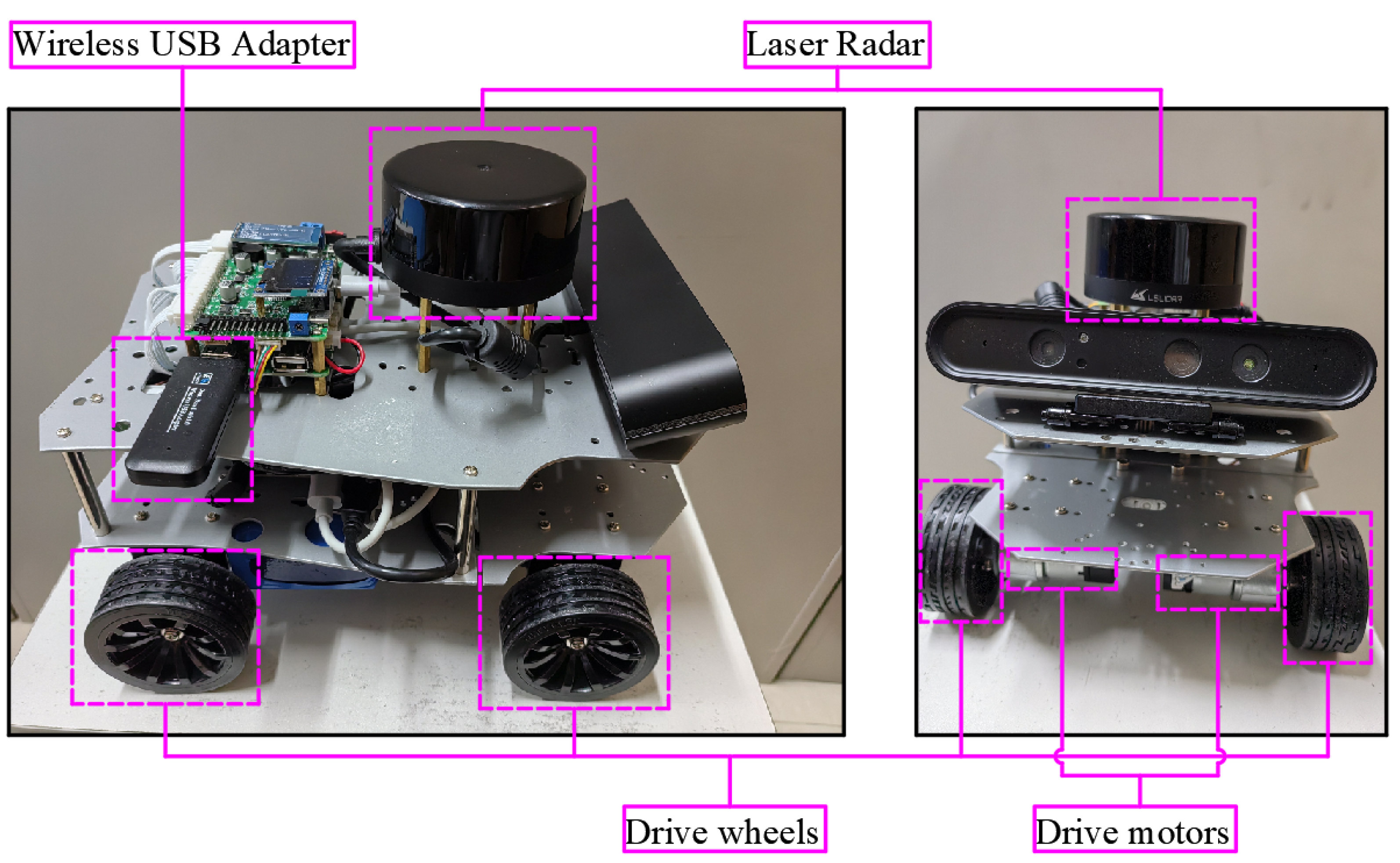
To validate the effectiveness of the EACI algorithm in a real-world environment, an experimental platform was constructed consisting of a Mini ROS vehicle (which produced by WHEELTEC Co., Ltd. of China in Dongguan) and a personal computer. As shown in Figure 31, the mini vehicle, measuring 265 mm × 205 mm × 195 mm, served as host computer, while the personal computer acted as the client computer. Both the host and the client were equipped with the 64-bit Ubuntu 18.04 operating system and the Robot Operating System (ROS), Melodic. Communication between the two was established via a Wi-Fi network using the SSH protocol, enabling remote control of the mini ROS vehicle through its IP address.

The schematic diagram of the Mini ROS vehicle is shown in Figure 31. The main control system of the Mini ROS vehicle includes an STM32 control board (model STM32F407VET6) equipped with an MPU9250 9-axis sensor, a Jetson Nano 4 GB board, a laser radar (M10P), four 12 V DC motors with Giant Magneto Resistance (GMR) encoders, a PlayStation 2 (PS2) wireless controller, and a wireless USB adapter. The laser radar is mounted on top of the vehicle at a height of 180 mm above the ground, and it is primarily used for environmental perception and obstacle detection. Detailed specifications are provided in

Table 4. Detailed parameter settings of the laser radar.

Item	Detection Range (m)	Distance Accuracy (cm)	Angular Resolution	Scan Frequency (Hz)	Field of View
Laser radar (M10P)	0.1–30	±3	0.22	12	360

.

After starting the Mini ROS vehicle, the PC connects to it via Wi-Fi and remotely logs into the vehicle system using the Secure Shell (SSH) protocol. The mapping program is launched by entering the command roslaunch turn_on_wheeltec_robot_mapping.launch. Then, a new terminal window is opened on the PC to start the Rviz visualization tool, and the PS2 wireless controller is used to control the vehicle’s movement. The Gmapping SLAM algorithm is employed to construct a grid map. The experimental area measures 480 cm × 300 cm and includes various obstacles, such as L-shaped, U-shaped, and cubic structures. The inner grid regions of the L-shaped and U-shaped obstacles are prone to causing deadlock in the ant colony algorithm, thus providing a suitable test scenario for verifying the proposed algorithm’s ability to avoid deadlocks. To ensure accurate map construction, each grid cell was set to a size of 5 cm × 5 cm. After completing the mapping process, the experimental environment map was exported using the map-saving package, the experimental environment and a map model generated by Laser Radar are displayed in Figure 32, where black areas represent obstacles and gray areas represent navigable regions.

In the experiment, the robot navigated fully autonomously using the algorithm proposed in this article. Its movement was controlled by a PID controller that followed the path generated by the algorithm. A position feedback system, based on the odometer, precisely measured the robot’s displacement using encoders and relayed this information back to the controller to ensure accurate path tracking.

The EACI algorithm was implemented as a plugin and integrated into the move_base package, with configuration managed through the move_base_params.yaml parameter file. After defining the start points and endpoints set on the map, the robot can execute path planning using the proposed algorithm. As shown in Figure 33, the DDMR successfully navigated along the designated navigation route and reached the destination without encountering deadlock grids. This finding highlights the robot’s strong navigation capabilities and further validates the effectiveness of the algorithm in specialized environments.

8. Conclusions

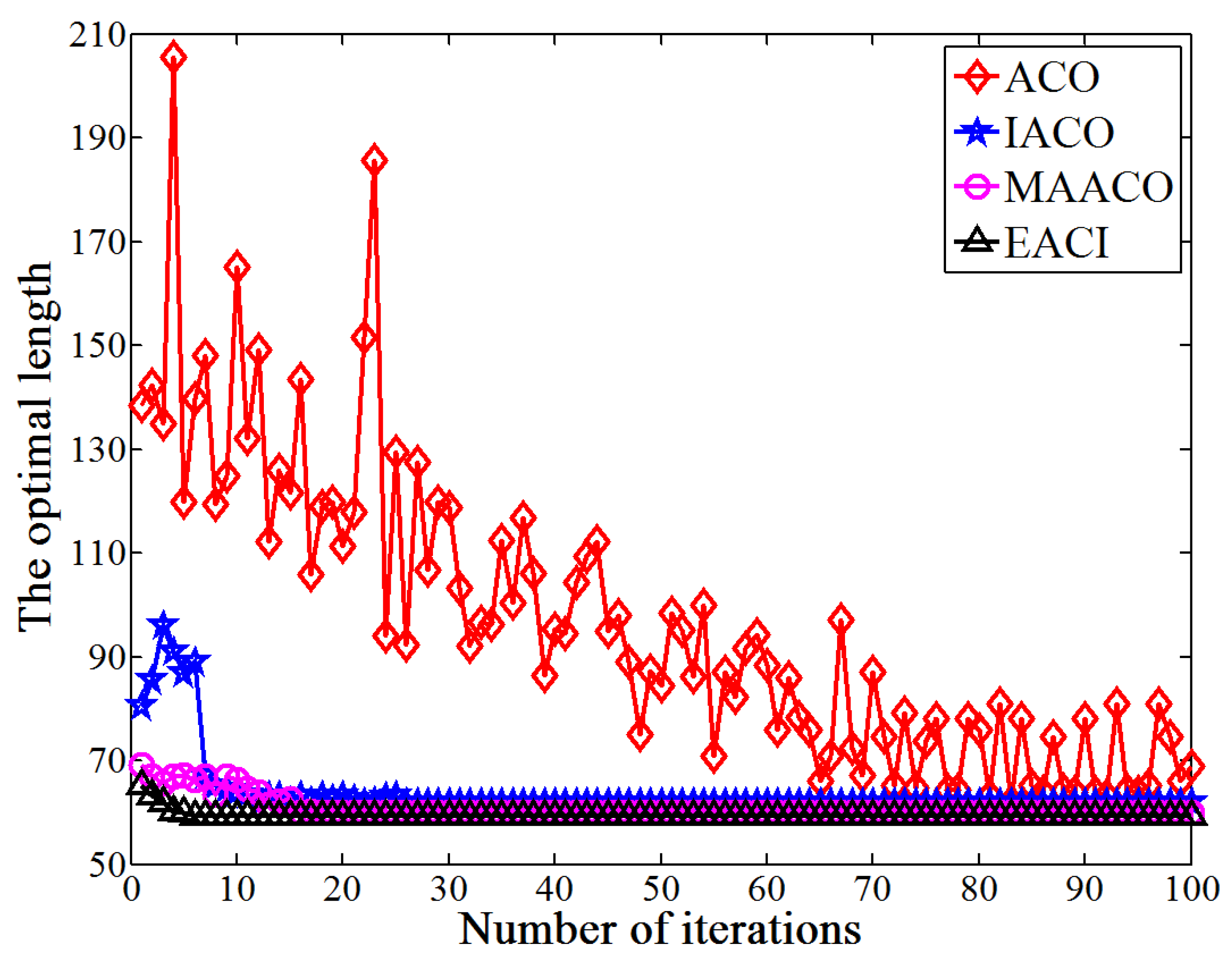
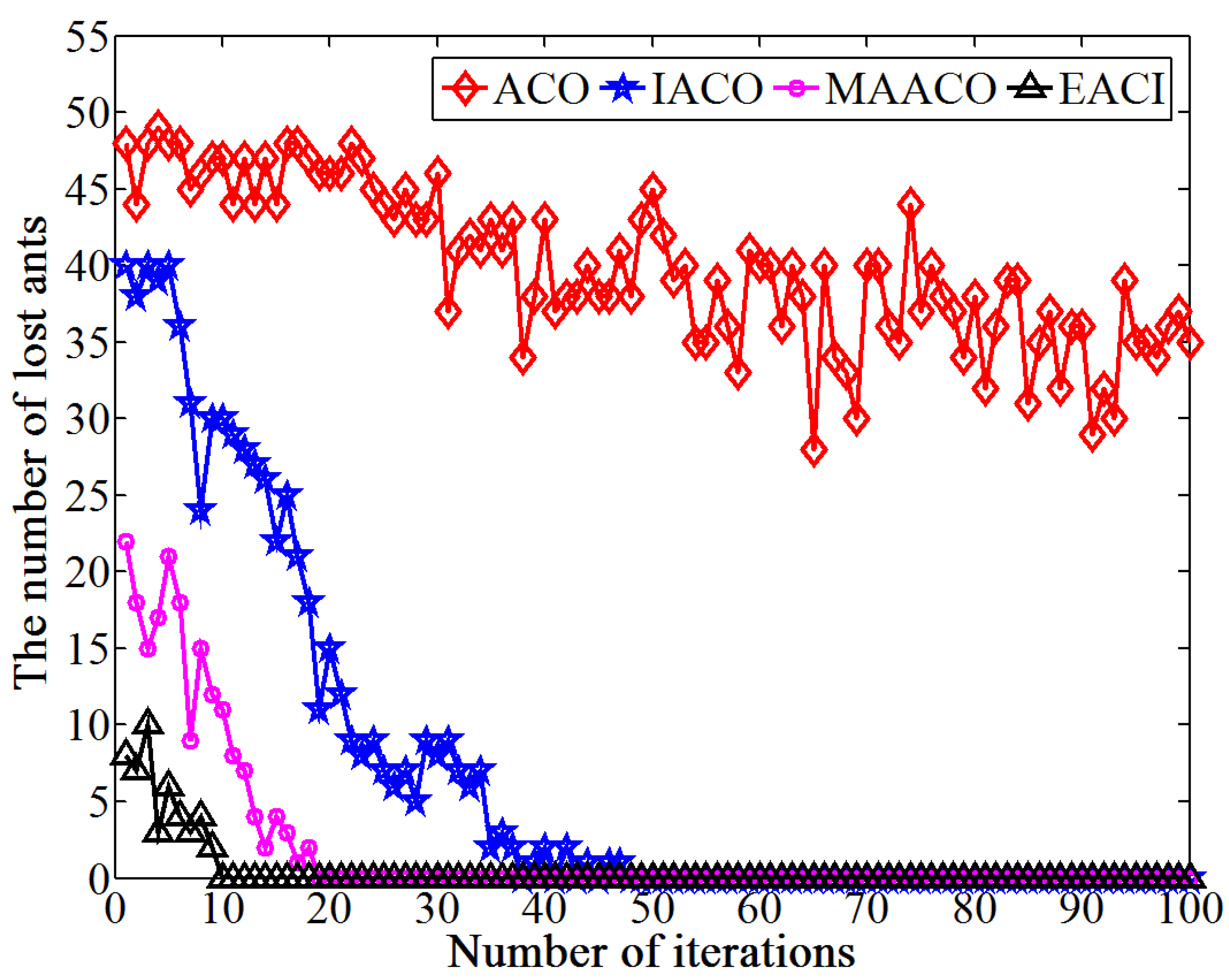
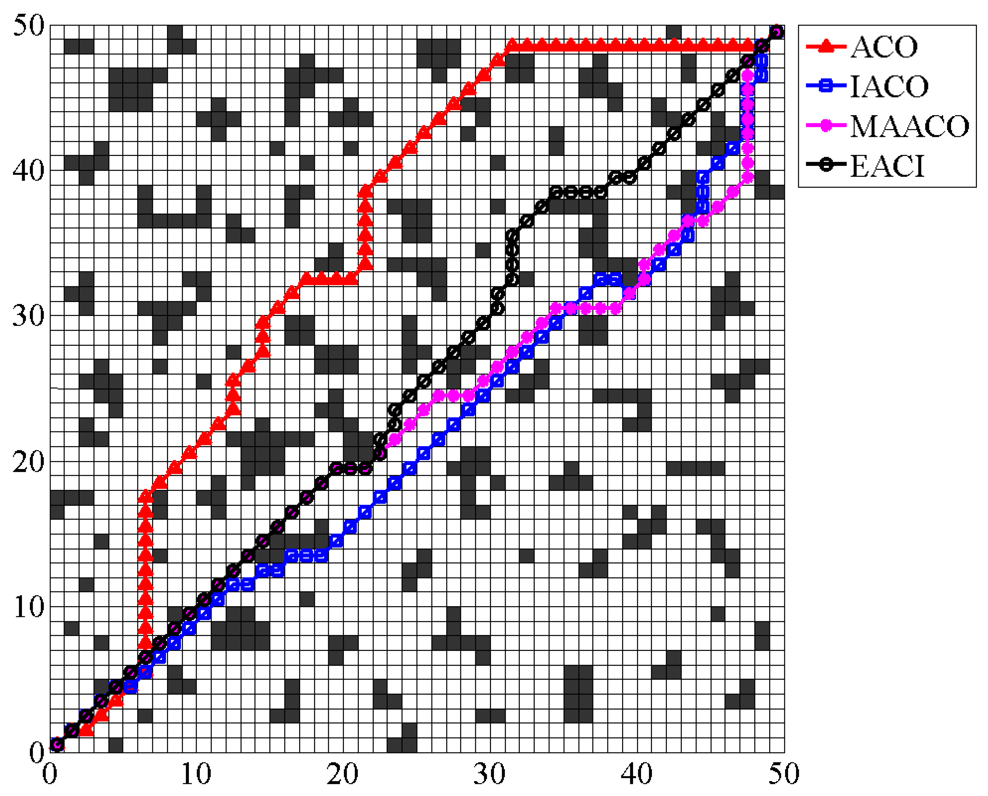
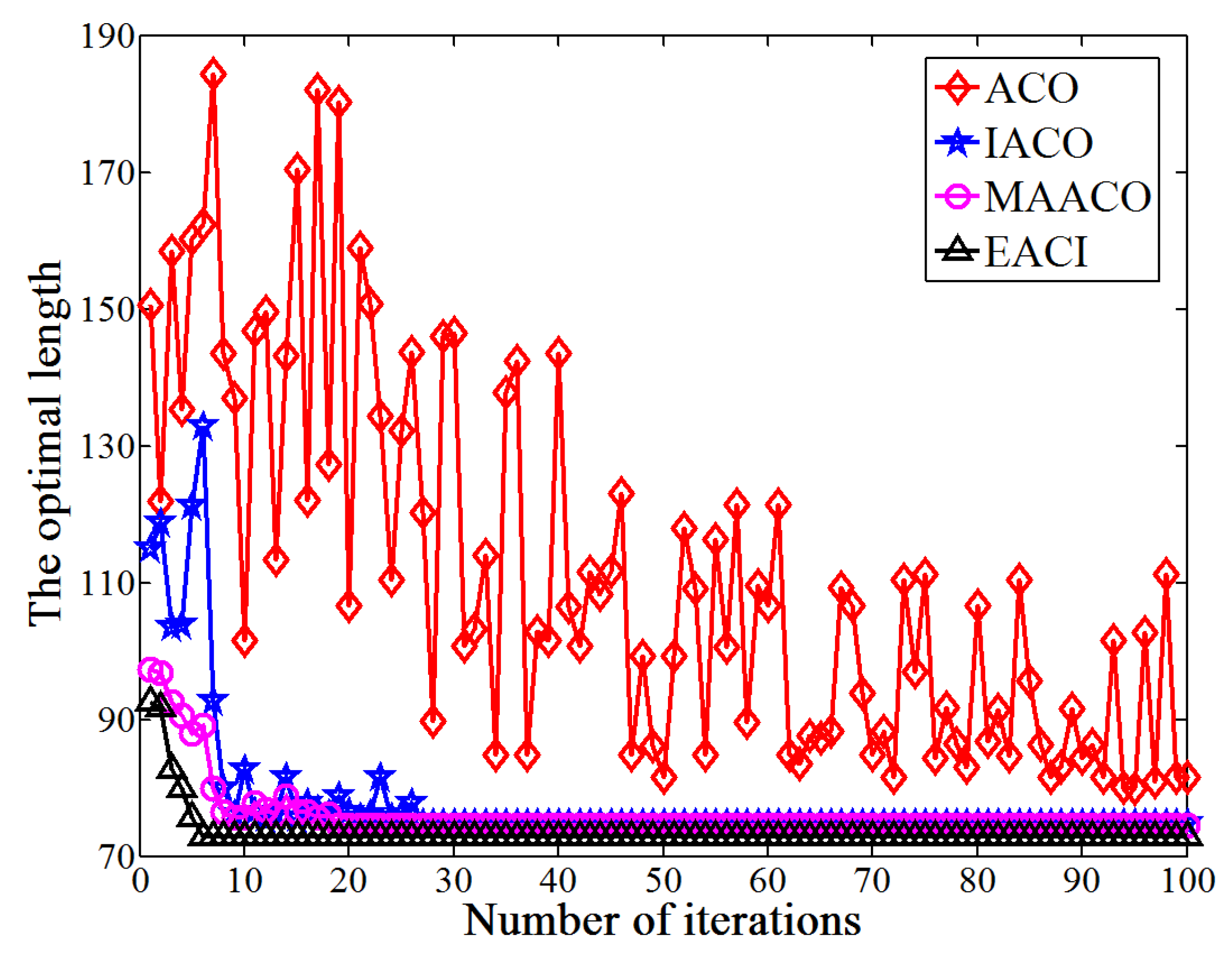
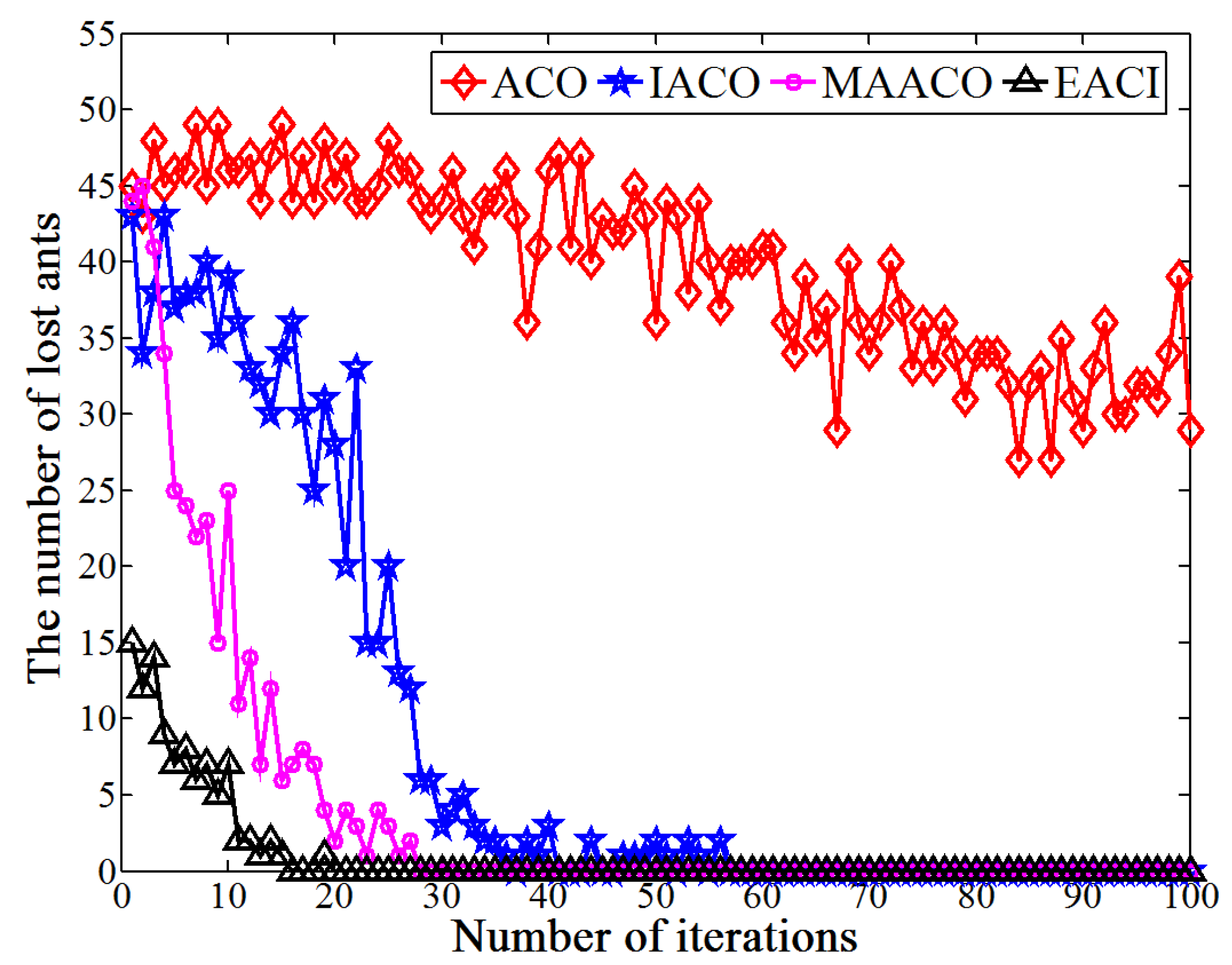
This study proposes an EACI algorithm for mobile robot path planning. The algorithm begins by preprocessing the original grid map to generate an auxiliary map, where multiple islands are evenly distributed between the starting and ending points. Non-uniform pheromones are then assigned between adjacent islands, the heuristic function is optimized, and an adaptive volatilization coefficient is introduced to dynamically update the pheromone level. Finally, the paths between adjacent islands are sequentially calculated and connected to form the global path planning scheme on the original map. In the 20 × 20 environment, the average number of iterations for EACI was only 1, representing reductions of 97.53%, 90.48%, and 84.38% compared to the ACO, IACO, and CMEACO algorithms, respectively. Meanwhile, the average number of lost ants was only 9.85, which was 99.21%, 94.28%, and 94.03% lower than that of ACO, IACO, and CMEACO, respectively. In the 30 × 30 environment, the average number of iterations for EACI was 1.4, exhibiting reductions of 98.18%, 93.61%, and 88.03% compared to ACO, IACO, and CMEACO, respectively, while the average number of lost ants was 27.5, representing reductions of 99.12%, 93.38%, and 88.43%. In the 40 × 40 environment, the average number of iterations for EACI was only 6.2, representing reductions of 93.8%, 76.25%, and 60.5% compared to ACO, IACO, and MAACO, respectively. Meanwhile, the average number of lost ants was only 47.6, which was 98.8%, 93.15%, and 74.85% lower than that of ACO, IACO, and MAACO, respectively. In the 50 × 50 environment, the average number of iterations for EACI was only 7.1, showing reductions of 92.9%, 74.54%, and 59.66% compared to ACO, IACO, and MAACO, respectively. At the same time, the average number of lost ants was only 99.2, which was 97.51%, 86.94%, and 74.85% lower than those of ACO, IACO, and MAACO, respectively. These results indicate that the EACI algorithm offers faster convergence and significantly fewer deadlock ants than other models, demonstrating its strong optimization performance. Moreover, real-world experiments confirm that the algorithm can quickly compute the navigation path from the starting to the endpoints, proving its practical application value.