A Riemannian Dichotomizer Approach on Symmetric Positive Definite Manifolds for Offline, Writer-Independent Signature Verification

Abstract

Automated handwritten signature verification continues to pose significant challenges. A common approach for developing writer-independent signature verifiers involves the use of a dichotomizer, a function that generates a dissimilarity vector with the differences between similar and dissimilar pairs of signature descriptors as components. The Dichotomy Transform was applied within a Euclidean or vector space context, where vectored representations of handwritten signatures were embedded in and conformed to Euclidean geometry. Recent advances in computer vision indicate that image representations to the Riemannian Symmetric Positive Definite (SPD) manifolds outperform vector space representations. In offline signature verification, both writer-dependent and writer-independent systems have recently begun leveraging Riemannian frameworks in the space of SPD matrices, demonstrating notable success. This work introduces, for the first time in the signature verification literature, a Riemannian dichotomizer employing Riemannian dissimilarity vectors (RDVs). The proposed framework explores a number of local and global (or common pole) topologies, as well as simple serial and parallel fusion strategies for RDVs for constructing robust models. Experiments were conducted on five popular signature datasets of Western and Asian origin, using blind intra- and cross-lingual experimental protocols. The results indicate the discriminative capabilities of the proposed Riemannian dichotomizer framework, which can be compared to other state-of-the-art and computationally demanding architectures.

1. Introduction

The adoption of biometric technology has become crucial in modern security and authentication systems [1,2,3]. Specifically, handwritten signatures hold particular significance due to their long-standing use in financial, legal, administrative, and forensic contexts [4,5,6,7]. They have been a key focus of biometric research for many years [8,9] due to their historical role in validating document authorship [10]. To this day, they remain a legally acknowledged method for verifying human identity in numerous types of transactions. Their sustained popularity is largely attributed to their simplicity and familiarity; individuals are accustomed to signing documents, whether through traditional pen-and-paper methods or modern electronic interfaces, such as touchscreens on smartphones and tablets [11]. However, the behavioral nature of handwritten signatures introduces a critical limitation: they are more vulnerable to forgery (F) compared to inherent physical characteristics, such as fingerprints or iris patterns. Skilled human forgers or computer-based presentation attackers can exploit the learned motor patterns of signatures to create convincing imitations.

Signature verification (SV) poses significant challenges, particularly for forensic-based applications. There is an increasing focus on developing automated signature verification (ASV) systems in order to accurately and efficiently differentiate between authentic and forged signatures as e-assistance for human intervention [5,12]. This binary classification task falls under the traditional scientific disciplines of computer vision and pattern recognition, requiring the ability to discern natural variations in handwriting from deliberate forgeries. It is a challenge compounded by factors such as the limited availability of handwriting features, the small number of genuine or bona fide (G) reference signatures, and the variability that exists (a) within an individual’s signatures samples (defined as the intra or the positive class ${\omega }^{+}$) and (b) between those of different individuals (defined as the inter- or negative class ${\omega }^{-}$).

To begin with, ASVs are categorized according to the way that the handwritten signature is acquired. There are two modes for signature acquisition: offline or static and online or dynamic. The online methods employ dynamic (i.e., time series) features by capturing multidimensional properties of the signature trace such as speed, pressure, pen inclination data, etc., all collected on appropriate platforms such as tablets and smart pens [13,14,15,16,17]. On the other hand, offline signature verification utilizes static signatures, represented and processed as grayscale, or binary, digital images. These signature images are compared through a series of procedures such as feature extraction, which is typically a mapping of the raw image to a mathematical vector space (i.e., the feature space), followed by the learning (i.e., training and validating) and testing stages of a binary classifier, or verifier. It is a fact that, nowadays, the use of contemporary machine learning and computer vision methods, such as those in [18,19,20,21,22,23,24,25], made OfSV systems both an efficient and practical aid, particularly for forensic applications and other related domains [4,6,12].

Another important categorization for SV systems is whether they follow the writer-dependent (WD) or the writer-independent (WI) framework. In the WD case, every new user enrollment needs a separate binary classifier to learn from the writer’s positive and negative samples [19,26,27]. The WI approach learns a universal model verifier, which tries to distinguish between similar and dissimilar pairs of images of a relatively large set of users, even with a few reference samples each [28,29,30]. It is a fundamental tenet of this framework that any verifier must compare pairs of signatures in order to ascertain their relative (dis)similarities. This process typically occurs in two stages. First, any signature image is embedded to the feature space under an appropriate coding scheme; this is formally termed the signature descriptor. In the second step, sets of (dis)similar descriptors emerging from signature pairs conditioned under the ${\omega }_{WI}^{\pm }$ classes are employed as inputs to the learning stage of the verifier model in order to accurately determine its optimal operating parameters. Finally, the resulting verifier model is tested against pairs of signatures that have never contributed to the learning stage in order to determine whether they came from the same author or not. WI is more challenging for accuracy; early attempts were not as effective as their WD counterparts. Therefore, WI systems have been the primary subject of recent works [18,23,30,31,32,33,34,35,36,37].

Although SV is generally acknowledged as a binary classification task, the discrimination between ${\omega }^{+}, {\omega }^{-}$ is affected by the way that the negative class${\omega }^{-}$ is represented. In the context of SV [38], at least two different kinds of forgeries are identified: the first is random forgery (RF) (or zero-effort forgeries or intrinsic failure) in which the negative class is represented by samples that originate from someone other than the authentic person (or an attacker). The second is skilled forgery (SF) or mimicry in terms of biometric presentation attacks. These samples incorporate a portion of knowledge of the signing process and usually exhibit greater resemblance to those of authentic users compared to random forgeries, which affects the accuracy of signature verifiers.

For the WI case, negative class representatives can originate either from random forgeries or skilled forgeries. For the WI verifier, the positive or similar class, denoted by${\omega }^{+}$, is represented by genuine-to-genuine (G-G) pairs. The negative or dissimilar class, denoted by ${\omega }^{-}$, can be represented either by genuine-to-random-forgery (G-RF) or genuine-to-skilled-forgery (G-SF) pairs or a mixture of them. Contrary to the restriction of the WD design stage, WI verifiers are allowed to utilize G-SF pairs only if the testing stage is blind or disjoint; that is, it tests pairs of signatures that do not contribute during the design-learning stage [28,39,40,41,42]. In this concept, an intuitively transfer learning approach by means of (a) a typical 5 $\times$ 2 internal fold and/or (b) a cross-lingual design-testing external protocol [18,19,35,37,43,44,45,46] can be applied without the concern of inducing bias to our system.

The WI-SV framework has been addressed under a number of “handcrafted”, as well as contemporary, deep neural topologies. Perhaps the most common “handcrafted” WI-SV topology utilizes the Dichotomy Transform (DT), a technique that transforms a Polychotomizer—or in the context of SV, a writer-dependent approach—into a simple Dichotomizer, enabling a writer-independent approach. For the last fifteen years [21,41], the DT has been applied for WI-SV purposes on a number of publications. Initially introduced by Cha and Srihari [47] at the beginning of the millennium, the DT converts feature vectors to distance vectors by means of a simple mathematical operation. In the following years, the works of Pezkalska and Duin [48,49], and Duin et al. [50], provided a theoretical foundation and justified the use of the dissimilarity space for recognition applications. Therefore, the DT is a legitimate candidate for designing WI-SV systems.

The process of verifying an individual’s signature is typically regarded as a visual recognition task. Up until now, any contemporary prevailing topologies, in addition to the previous utilization of the DT, were predicated on the underlying assumption that the data in the form of the signature descriptors form a vector space which complies with Euclidean space axioms [51]. But now, there is evidence that ignoring the geometrical properties of the data is restrictive [51]. Recently, a number of methodologies have been proposed for WI-SV that adhere to the assumption that the signature descriptors comply with geometrically curved spaces [52,53,54,55,56]. Specifically, the signature descriptors, in the form of signature covariance matrices, are considered to be points that belong to the Symmetric Positive Definite (SPD) ${\mathit{P}}_d$ manifold, a subset of the native vector space ${\mathbb{R}}^{d\times d}$. Therefore, inspired by (a) the use of the DT on signature verification and (b) the success of applying geometrically inspiring algorithms which exploit curved spaces, this work provides a comprehensive mathematical framework regarding the use of an equivalent expression of the Dichotomy Transform in curved and non-Euclidean spaces. The objective of this work is to clearly show that simple Riemannian approaches, compared to computationally intense verifiers, can provide low verification errors as well. Bearing in mind that we consider the term dissimilarity to relate to the Dichotomy Transform, by means of the subtraction operator and not to the distance between two entities, the main contributions of this paper are below:

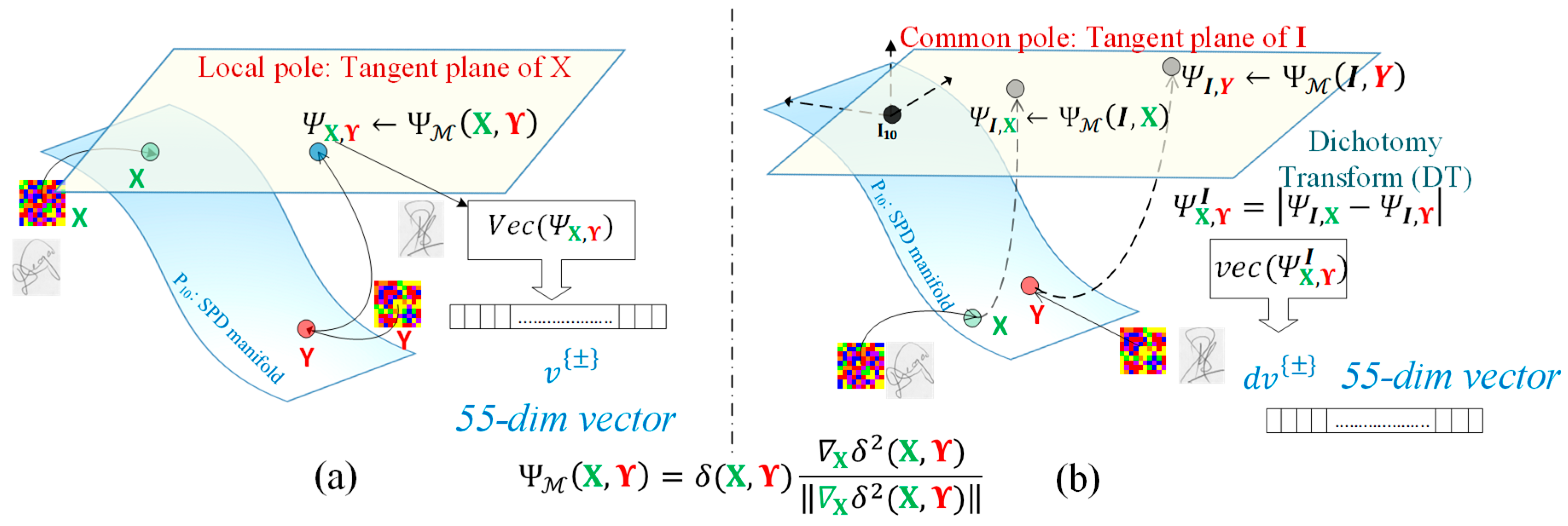
• We provide a mathematical framework for modeling the leap from the Euclidean-oriented DT to its Riemannian equivalent, Riemannian dissimilarity vectors (RDVs) $\Psi$, which are employed for the first time in the literature for addressing WI-SV. The Euclidean-oriented DT is typically performed with the use of the subtraction operator $(-)$ between vector descriptors. In the context of the Riemannian framework, the concept of a bipoint, i.e., oriented pairs of points, which is an antecedent of a vector, offers a novel perspective on the interpretation of subtractions [57]. As a result, the proposed RDVs $\Psi$ are formed as the result of the Riemannian equivalent for vector space subtraction between two SPD manifold entities $\Psi \leftarrow ({\mathit{X}-\mathit{Y})}_{\mathcal{M}}$. The RDVs $\Psi$ are expressed by a manifold dissimilarity function, $\Psi \leftarrow {\Psi }_{\mathcal{M}}\left(\cdot ,\cdot \right): {\mathit{P}}_d\times {\mathit{P}}_d\to {\mathcal{T}}_{{\mathit{P}}_d}$, which is a map to the tangent bundle of the SPD manifold. For classification tasks, the resulting RDVs (in the form of symmetric matrices) are converted to a vectored from ($v_{\mathit{X},\mathit{Y}}$ or ${dv}_{\mathit{X},\mathit{Y}}$) with the use of a vector operator ${vec}_{\left(\mathit{{\rm I}}\right)}\left(\Psi \right)$.
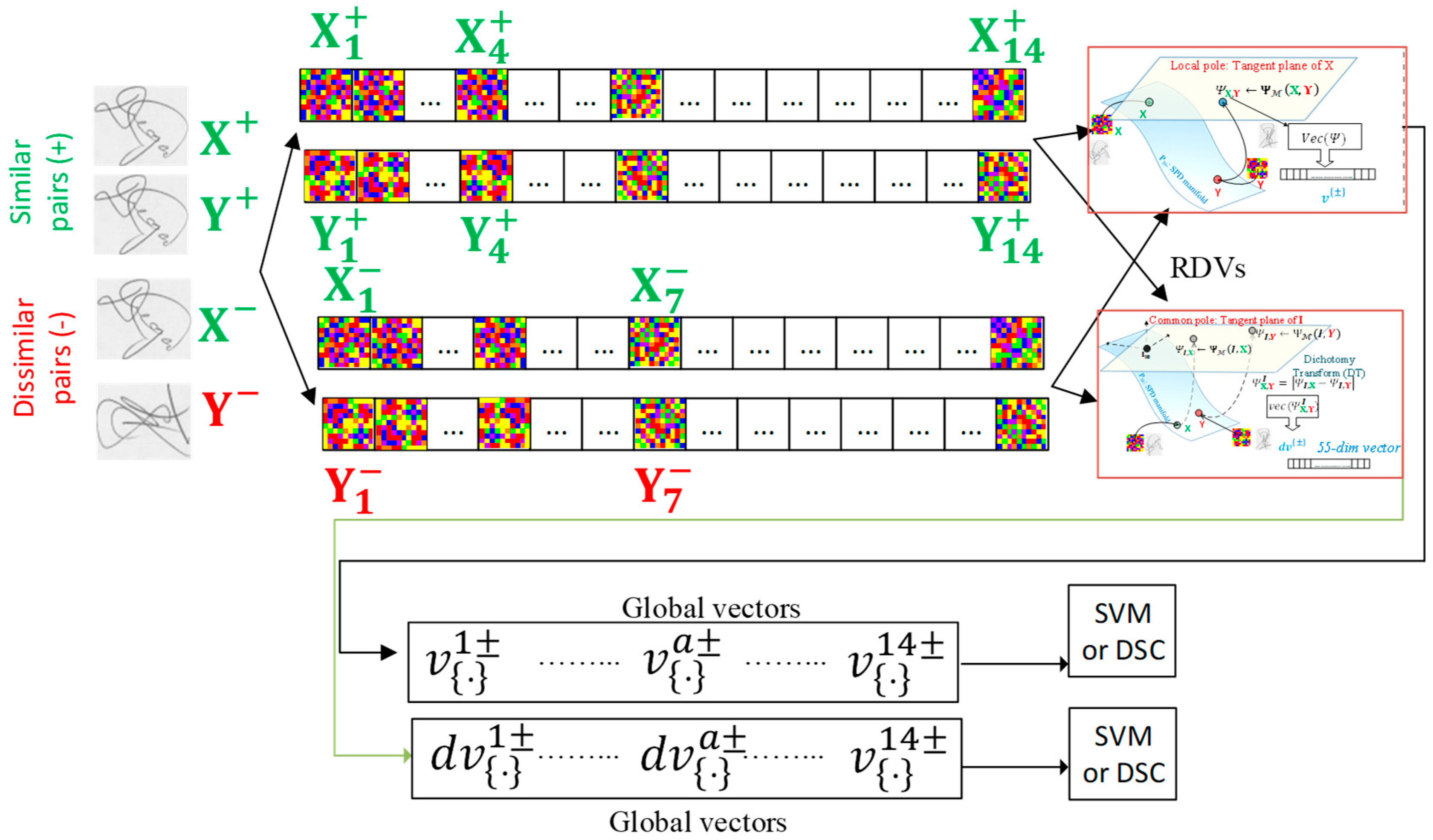
• We present and compare two alternative methodologies for constructing the RDVs between two signature covariance matrices, $\mathit{X},\mathit{Y}$, namely the local and the global common pole approach. In the case of the local approach, the RDV is formed by the local tangent vectors ${\Psi }_{\mathit{{\rm X}},\mathit{Y}} ϵ{\mathcal{T}}_{\mathit{X}}$. Intuitively, the local RDV approach encodes the notion of the dissimilarity between $\mathit{X},\mathit{Y}$ by means of an appropriate subtraction operation (${\mathit{X}-\mathit{Y})}_{\mathcal{M}}\to {\Psi }_{\mathit{X},\mathit{Y}} ϵ{\mathcal{T}}_{\mathit{X}}$. In the case of the global common pole approach, the ${\mathit{I}}_d$ common pole is used to evaluate the RDV dissimilarity (${\mathit{I}-\mathit{X})}_{\mathcal{M}}\to {\mathsf{\Psi }}_{\mathit{I},\mathit{X}} ϵ{\mathcal{T}}_{\mathit{I}}$, (${\mathit{I}-\mathit{Y})}_{\mathcal{M}}\to {\Psi }_{\mathit{I},\mathit{Y}} ϵ{\mathcal{T}}_{\mathit{I}}$ for each one of the $\mathit{X},\mathit{Y}$ with respect to the identity matrix ${\mathit{I}}_d$. Then, the Euclidean-based DT, applied directly to the ${\Psi }_{\mathit{I},\mathit{X}}$, ${\Psi }_{\mathit{I},\mathit{Y}}$, evaluates the global common pole RDV ${\Psi }_{\mathit{{\rm X}},\mathit{Y}}^{\mathit{I}}=\left|{\Psi }_{\mathit{I},\mathit{X}}-{\Psi }_{\mathit{I},\mathit{Y}}\right|$. To both local and global common pole RDVs, we then apply the ${vec}_{\left(\mathit{{\rm I}}\right)}\left(\Psi \right)$ operator in order to create any of the two $v$ or $dv$ vectored forms for classification purposes.
• We employ and compare the efficiency of the RDVs under two different popular frameworks in order to realize the WI-SV system. The first one consists of a binary support vector machine (SVM), while the second utilizes a decision stump learning algorithm equipped with a Decision Stump Committee (DSC) structure under the Gentle Ada Boost framework initially proposed by [28] and among others employed also for WI-SV purposes in [37]. The experimental setup consists of blind disjoint learning $\mathbb{L}$ and testing $\mathbb{T}$ sets in both intra-lingual and cross-lingual test sets.
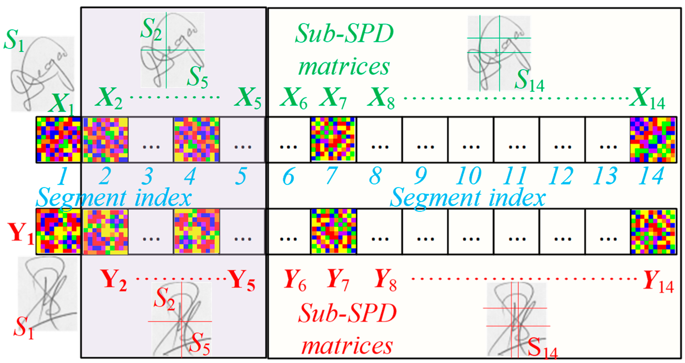
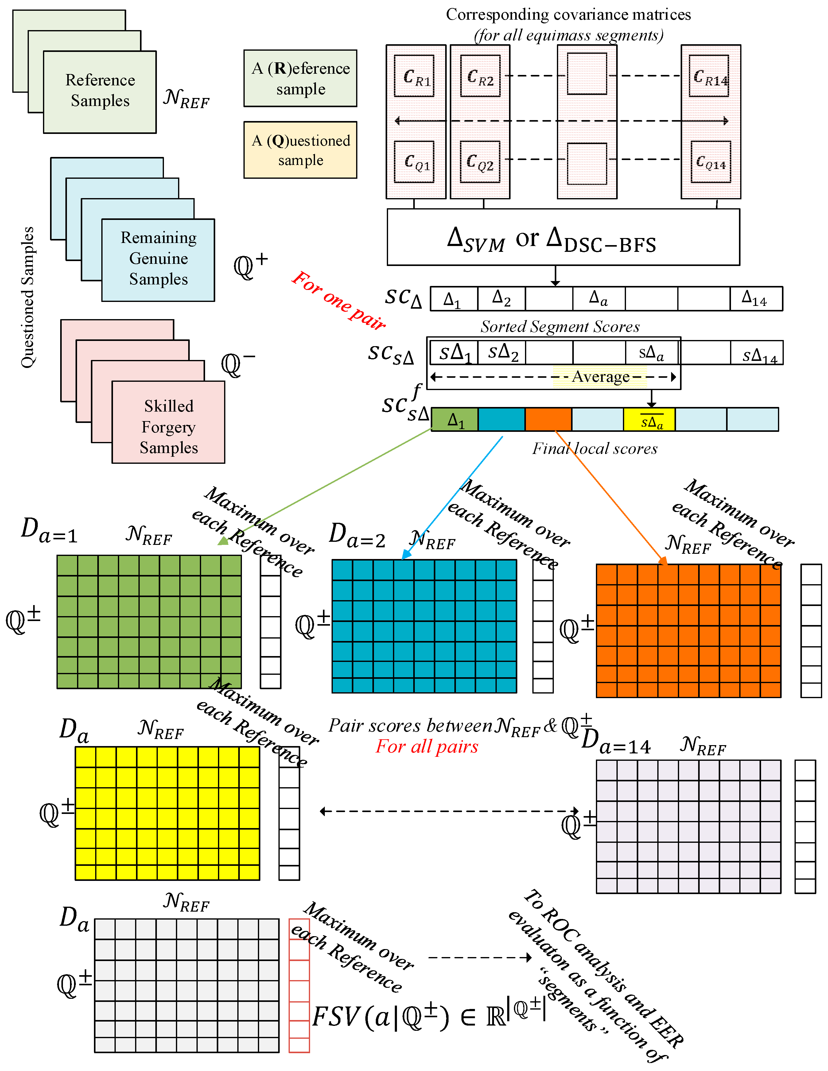
• We follow two distinct methodologies for the purpose of fusing the resultant local $v$ or global common pole $dv$. For this purpose, related coordinates between equimass spatial segments $S$ between a pair of signature images ${\mathit{I}\mathit{m}\mathit{g}}_{\mathit{X}},{\mathit{I}\mathit{m}\mathit{g}}_{\mathit{Y}}$ are selected; thus, a pair of covariance matrices, ${\mathit{X}}_S,{\mathit{Y}}_S$, is evaluated for any two visual segments. Then, the local ${\Psi }_{\mathit{{\rm X}},\mathit{Y}}$or common pole ${\Psi }_{\mathit{{\rm X}},\mathit{Y}}^{\mathit{I}}$ RDVs of a sequence of image segments can be fused under two modes: (a) a serial one, in which the resulting scores from each segment are combined in order to create a score as a function of the segments and (b) a parallel one in which vectored forms $v$ or $dv$ are appended in order to form an extended vector with larger dimensionality, accompanied by one score.

The remainder of this paper is organized as follows: Section 2 provides a summary of the literature regarding WI-SV and introduces the key elements of the proposed idea. Section 3 outlines the SPD manifold accompanied by the theoretical elements and mathematical tools of the proposed methodology. Section 4 provides details regarding the experimental protocol, and Section 5 displays the corresponding experimental results. Finally, conclusions are drawn in Section 6. Our source code will become available at https://github.com/ezois/RDV (accessed on 26 May 2025) for reproducibility purposes.

2. WI-SV-Related Work and Overview

2.1. Related Work

As earlier stated, perhaps the most popular strategy for the implementation of WI-SV systems was dissimilarity mapping induced by the Dichotomy Transform. Given a pair $(a,b)$ of signature images and their corresponding descriptors, $f_a, f_b\in {\mathbb{R}}^d$, the DT, initially proposed in [47], utilizes a dissimilarity function, ${\Psi }_{\mathit{Euc}}\left(\cdot ,\cdot \right): {\mathbb{R}}^d\times {\mathbb{R}}^d\to {\mathbb{R}}_{+}^d$, which maps to a dissimilarity space, $\mathcal{D}\subseteq {\mathbb{R}}_{+}^d$, by means of the following expression: $\mathcal{D}=\left|f_a-f_b\right|$. By using the DT, a Polychotomizer is transformed into a Dichotomizer through the introduction of the concept of “dissimilarity” between samples of the same and different classes. As a consequence, the similar (${\omega }^{+}$) or dissimilar $({\omega }^{-}$) classes are independent of the number of writers involved. This attribute renders the design process intuitive, and it can be applied in a direct transfer learning framework. Feature dissimilarities were used in [41] under a framework which combines graphometric feature sets and an ensemble of classifiers. Following reference [28], the DT was employed under a multiple feature extraction method and a global boosting feature selection. The dissimilarity space was also used in the development of a hybrid WI-WD system in [29]. Partially oriented features were also enabled under the DT framework, with notable success in both blind intra- and cross-lingual experiments [37]. The use of the DT and data-driven features was originally introduced in [58], in which an SVM classifier acted as the training model. In [30], the use of the DT was further augmented by the introduction of a white-box analysis at the instance level using the instance hardness measure. In [59], the DT is utilized with the 256 Local Binary Patterns (LBP) features and a decision tree classifier. All the aforementioned methodologies adhere to the assumption that the feature space—data under examination—follow the vector space axioms, i.e., closed under vector addition and scalar multiplication.

In recent times, there has been a growing application of geometrically preserving SV systems in a number of research endeavors. All of these methods rely on the use of Symmetric Positive Definite (SPD) matrices as image descriptors, with considerable success in discrimination [60,61]. It has been demonstrated that SPD matrices are an effective means of authenticating signatures in both WD [52] and WI modes [54,55,56], while in [6,38,39] metric learning approaches have been enabled in a WI framework with significant success in both intra- and cross-lingual scenarios.

2.2. Overview of the Proposed Method

This section is devoted to a brief description of the proposed system, with emphasis on the learning stage. Figure 1 provides the key point RDV concept of the proposed method through a graphical depiction of a toy example. Let us consider a pair of static handwritten signature images and the corresponding covariance descriptors $\mathit{X},\mathit{Y}$ of either the entire images or any equimass segment (denoted by an index $a$). Both ${\mathit{X}}_{\mathit{a}},{\mathit{Y}}_{\mathit{a}}$ are regarded as points on the SPD manifold ${\mathit{P}}_{10}$. Subsequently, two distinct frameworks are established in order to contextualize the concept of dissimilarity between the aforementioned covariance matrices. In the first one (local approach), the Riemannian dissimilarity vector is a symmetric matrix $\Psi \mathsf{ϵ}{\mathbb{R}}^{10\times 10}$, which lies on the local tangent plane ${\mathcal{T}}_{\mathit{X}}$. The evaluation of the RDV $\Psi$ inherently utilizes (a) a specific manifold metric $\delta$ and (b) the manifold equivalent ${(-)}_{\mathcal{M}}$ of the Euclidean subtraction operator ${\left(-\right)}_{Euc}$. Details regarding $\delta$ and ${(-)}_{\mathcal{M}}$ shall be provided in the subsequent paragraphs. A $vec(\cdot )$ operator aligns the symmetric matrix $\Psi$ (i.e., the tangent vector) to a typical vectored form $v_{\mathit{X},\mathit{Y}}\mathsf{ϵ}{\mathbb{R}}^{55}$. In the second approach, the evaluation of the RDVs ${\Psi }_{\mathit{I},\mathit{X}}$ and ${\Psi }_{\mathit{I},\mathit{Y}}$ is made with respect to the ${\mathbf{I}}_{10}$ common pole followed by (a) the Euclidean-based Dichotomy Transform defined as ${\Psi }_{\mathit{{\rm X}},\mathit{Y}}^{\mathit{I}}=\left|{\Psi }_{\mathit{I},\mathit{X}}-{\Psi }_{\mathit{I},\mathit{Y}}\right|$ and (b) a $vec(\cdot )$ operator, which creates the $d{v}_{\mathit{X},\mathit{Y}}\mathsf{ϵ}{\mathbb{R}}^{55}$ vectored forms.

The aforementioned elementary building blocks (a, b) of Figure 1 create the $v_{\mathit{X},\mathit{Y}}$ or ${dv}_{\mathit{X},\mathit{Y}}$ vectors, which in their turn inherently express the dissimilarity between a pair of SPD matrices. Figure 2 illustrates the process of decomposing a static signature image into an array of fourteen covariance matrices, with each matrix corresponding to either the entire image or a specific segment indexed by $a=1:14$. It is easy to conceive that for a pair $({Img}_X,{Img}_Y)$ of handwritten signatures, two arrays of covariance matrices ${\mathit{X}}_{\mathit{a}},{\mathit{Y}}_{\mathit{a}}$ are extracted; consequently, for each segment pair ${\mathit{X}}_{\mathit{a}},{\mathit{Y}}_{\mathit{a}}$, a Riemannian dissimilarity vector $v_{\{kind of measure\}}^a$ or $d{v}_{\{kind of measure\}}^a$ can be created. According to the discussion in the introduction, the pairs of ${\mathit{X}}_{\mathit{a}},{\mathit{Y}}_{\mathit{a}}$ can originate either from the positive or the negative class ${\mathit{X}}_a^{\pm },{\mathit{Y}}_a^{\pm }$ and create the corresponding ${\Psi }_{{\mathit{X}}_a^{\pm },{\mathit{Y}}_a^{\pm }}$ and $v_{\{\cdot \}}^{a\pm }$ or ${\Psi }_{{\mathit{X}}_a^{\pm },{\mathit{Y}}_a^{\pm }}^{\mathit{I}}$ and ${dv}_{\{\cdot \}}^{a\pm }$. In this work, two individual learning frameworks are explored according to the fusion strategy followed.

Figure 3 depicts the first one, tagged hereafter as the local LFW1. Sets comprising positive (G-G) and negative (G-RF or G-SF) pairs form the corresponding sets of RDVs and $v_{{\mathit{X}}_1^{\pm },{\mathit{Y}}_1^{\pm }}$ or ${dv}_{{\mathit{X}}_1^{\pm },{\mathit{Y}}_1^{\pm }}$. Then, two different classifiers, a binary support vector machine and a Decision Stump Committee, are trained and validated in order to select the optimal parameters of each one. It must be made clear here that the LFW1 learning procedure of both the SVM and DSC classifiers involves only the first ${\mathit{X}}_1^{\pm },{\mathit{Y}}_1^{\pm }$ covariance matrix, which corresponds to the entire image; i.e., the remaining segments are not utilized during the learning stage.

Figure 4 depicts the second learning framework, tagged as the parallel LFW2. Again, sets comprising positive (G-G) and negative (G-RF or G-SF) deliver the corresponding $v_{\{\cdot \}}^{a\pm }$ or ${dv}_{\{\cdot \}}^{a\pm }$ over all $a$ -segments. Thus, in LFW2, a vector of higher dimensionality is formed by concatenating all the corresponding vectors $\left\{v_{\{\cdot \}}^{a\pm }\right\}$ or $\left\{{dv}_{\left\{\cdot \right\}}^{a\pm }\right\}, a=1:14$ as $\left[v_{\{\cdot \}}^{1\pm }\dots v_{\{\cdot \}}^{a\pm }\dots v_{\{\cdot \}}^{14\pm }\right]$ or $\left[{dv}_{\{\cdot \}}^{14\pm }\dots {dv}_{\{\cdot \}}^{a\pm }\dots {dv}_{\{\cdot \}}^{14\pm }\right]$. Then, the SVM and DSC classifiers are subjected to the same learning procedure in order to select their optimal operating parameters. Details regarding the learning and testing procedure are provided in the subsequent paragraphs.

3. Materials and Methods

Although already used in the previous sections, the following essential notations are introduced from this point on: Matrices are denoted by upper case letters (e.g., $X\in {\mathbb{R}}^{d\times d}$). When deemed necessary, this also denotes symmetric matrices (e.g., $T\in {\{S}_d\}$), while vectors are denoted by lowercase letters (e.g., $x\in {\mathbb{R}}^d$). With the notation ${(\cdot )}_{ij}$, we denote the $\left(i,j\right)$-entry of any matrix. Finally, SPD matrices are denoted by bold, uppercase letters (e.g., $\mathit{X}\in {\mathit{P}}_d$).

3.1. Theoretical Elements and Mathematical Tools of the SPD Manifold

The symmetric positive definite manifold ${\mathit{P}}_d$ is the set of all real matrices $\left\{\mathit{X}\in {\mathbb{R}}^{d\times d}\right\}$ such that the matrix is symmetric $\mathit{X}-{\mathit{X}}^{\prime }=0$ and strictly positive, ${\mathit{v}}^{\prime }\mathit{X}v>0,\forall v\in {\mathbb{R}}^d\setminus \left\{0^d\right\}$. Intuitively, points that belong to the SPD manifold are contained within the interior of a convex cone in a $n(n+1)$/2 dimensional Euclidean space. The tangent space ${\mathcal{T}}_{\mathit{X}}$ at any manifold point $\mathit{X}\in {\mathit{P}}_d$ is the set of symmetric matrices $\Psi \in {\{S}_d\}$, and it comprises all the possible derivatives (i.e., the tangent vectors) on the manifold at $\mathit{X}$; therefore, ${\mathcal{T}}_{\mathit{X}}$ is a vector space. The SPD is a Riemannian manifold; thus, it is a differentiable manifold equipped with a smoothly varying inner product ${〈\cdot ,\cdot 〉}_{\mathit{X}}$. The geometric perspective of the SPD manifold is endowed with the use of a Riemannian metric (or norm) of a tangent vector $\Psi \in {\mathcal{T}}_{\mathit{X}}$, defined by ${‖\Psi ‖}_{\mathit{X}}^2={〈\Psi ,\Psi 〉}_{\mathit{X}}$. On the SPD manifold and its tangent plane on point $\mathit{X}$, two mappings are defined: the first is the exponential map ${\mathit{exp}}_{\mathit{X}}\left(\Psi \right):{\mathcal{T}}_{\mathit{X}}\to {\mathit{P}}_d$, in which a tangent vector, $T$, with origins in a manifold point (or pole),$\mathit{X}$, is projected back on the manifold; the second is the logarithmic map, ${\mathit{log}}_{\mathit{X}}\left(\mathit{T}\right)={exp}_{\mathit{X}}^{-1}\left(\mathit{T}\right):{\mathit{P}}_d{\to \mathcal{T}}_{\mathit{X}}$, which projects a manifold point, $\mathit{T}$, to the local tangent plane of the pole, $\mathit{X}$, by means of its local tangent vector, $T$. The logarithmic map is considered to be the equivalent ${(-)}_{\mathcal{M}}$ of the Euclidean subtraction operator $(-)$ [57].

A Riemannian metric is defined as a smoothly varying inner product on the tangent space at each point of the manifold. The Riemannian metric is of particular interest since it is employed to measure arc lengths upon the manifold. A curve of zero acceleration that connects two points, $\mathit{X}$ and $\mathit{Y}$, in the SPD manifold is called a geodesic, and it is analogous to straight lines in ${\mathbb{R}}^d$, while its length is called the geodesic distance. The geometric perspective of the SPD manifold is often endowed with the use of the related Affine Invariant Riemannian Metric (AIRM) [57], defined for $\mathit{X}\in {\mathit{P}}_d$ and $Y,W\in {\mathcal{T}}_{\mathit{X}}$ as follows:

$${〈Y,W〉}_{\mathit{X}}\triangleq 〈{\mathit{X}}^{-1/2}Y{\mathit{X}}^{-1/2},{\mathit{X}}^{-1/2}W{\mathit{X}}^{-1/2}〉=Tr\left({\mathit{X}}^{-1}Y{\mathit{X}}^{-1}W\right)$$

(1)

which induces the notion of a distance, formally termed geodesic distance ${\delta }_g(\cdot ,\cdot )$:${\mathit{P}}_d\times {\mathit{P}}_d\to {\mathbb{R}}^{+}$, between the manifold points $\mathit{X},\mathit{Z}\in {\mathit{P}}_d$ as

$${\delta }_g\left(\mathit{X},\mathit{Z}\right)={‖{\mathit{l}\mathit{o}\mathit{g}\mathit{m}(\mathit{X}}^{-1/2}\mathit{Z}{\mathit{X}}^{-1/2})‖}_F$$

(2)

where $logm$ is the matrix logarithm function expressed by

$$logm\left(\mathit{X}\right)=\mathit{U}diag\left(\log {(\lambda }_{\mu })\right){\mathit{U}}^{\prime }$$

(3)

and ${\lambda }_{\mu }$ is the $\mu$-th eigenvalue, $\mu =1:d$, derived from the eigenvalue analysis of$\mathit{X}=\mathit{U}diag\left({\lambda }_{\mu }\right){\mathit{U}}^{\prime }$.

The geodesic distance ${\delta }_g$ is considered to be the most popular distance measure in the SPD manifold. In addition, a number of metrics or divergences can also be defined over the SPD manifold. In this work, we also exploit two additional symmetric Bregman divergences to act as distance measures between two points on the SPD manifold. The first is the Stein [62] divergence, ${\delta }_{St}: {\mathit{P}}_d\times {\mathit{P}}_d\to {\mathbb{R}}^{+}$, defined by

$${\delta }_{St}^2\left(\mathit{X},\mathit{Z}\right)=\mathit{ln}\mathit{det}\left({\displaystyle \frac{\mathit{X}+\mathit{Z}}{2}}\right)-{\displaystyle \frac{1}{2}}\mathit{ln}\mathit{det}\left(\mathit{X}\mathit{Z}\right)$$

(4)

while the second is the Jeffrey or symmetric KL [63] divergence ${\delta }_J: {\mathit{P}}_d\times {\mathit{P}}_d\to {\mathbb{R}}^{+}$ defined by

$${\delta }_J^2\left(\mathit{X},\mathit{Z}\right)={\displaystyle \frac{1}{2}}Tr\left({\mathit{X}}^{-1}\mathit{Y}\right)+{\displaystyle \frac{1}{2}}Tr\left({\mathit{Y}}^{-1}\mathit{X}\right)-d$$

(5)

3.2. Euclidean and Riemannian Dissimilarity Frameworks

The formulation of the abstract concept of the proposed RDV for WI-SV purposes necessitates an elucidation of the association between the formation of difference vectors in both vector space methods and those based on Riemannian manifolds. This is achieved by following a historical roadmap, which mainly follows the steps of [51,64]. To begin, let us consider the data matrix $X\in {\mathbb{R}}^{d\times k}:={\left\{x_i\right\}}_{i=1}^k, x_i\in {\mathbb{R}}^d$ comprised of a set of vectors (or descriptors). Gaussian mixture models (GMMs) have been proposed as a probabilistic approach for representing the $x_i$ data instances. In detail,

$$p\left(x_i|\lambda \right)={\sum }_{j=1}^N{\pi }_j\mathcal{N}\left(x_i|{\mu }_j,{\mathit{C}}_j\right)$$

(6)

in which $\lambda =\{{\pi }_j,{\mu }_j,{\mathit{C}}_j\}$ represents the mixing probability, the mean, and the covariance of each one of the $j$-th corresponding Gaussian factors. In view of the fact that in the field of statistics a score function is defined as the log-likelihood of the data on the model, the Fisher Vectors (FVs) encode the data through the use of the GMM score function. The gradient with respect to the mean, ${\mu }_j$, is expressed as

$${\nabla }_{{\mu }_j}\log p\left(X|\lambda \right)={\sum }_{i=1}^N{\gamma }_j\left(x_i\right){\mathit{C}}_{\mathit{j}}^{-1}{\gamma }_j\left({{\mu }_j-x}_i\right)$$

(7)

where the term ${\gamma }_j\left(x_i\right)$ represents the soft assignment of the $x_i$ vector to the corresponding $j$-th Gaussian factor

$${\gamma }_j\left(x_i\right)={\displaystyle \frac{{\pi }_j\mathcal{N}\left(x_i|{\mu }_j,{\mathit{C}}_j\right)}{{\sum }_{i=1}^N{\pi }_j\mathcal{N}\left(x_i|{\mu }_j,{\mathit{C}}_j\right)}}$$

(8)

Jégou et al. [65] simplified the FV by proposing the Vector of Locally Aggregated Descriptors (VLAD) encoding. This was made by (a) having the covariance matrices ${\mathit{C}}_j$ be fixed and diagonal and (b) exploiting a hard assignment of the local descriptors instead of the soft ones in FVs. By dropping the normalization terms of the Gaussian function, VLAD evaluates the gradient of the Euclidean distance. In other words, given a set $d_j\in {\mathbb{R}}^d$ of points in a vector space by means of a dictionary $\mathfrak{D}\in {\mathbb{R}}^{N\times d},\mathfrak{D}={\left\{d_j\right\}}_{j=1}^N$, any query set of vectors $X^Q$ comprising the $x_i^Q\in {\mathbb{R}}^d$ query vectors is encoded with the concatenation of $N$-local difference vectors (LDV) $v_j^{Euc}$ by accumulating the differences between a query $x_i^Q$ and a center $d_j$ according to the following:

$$v_j^{Euc}={\sum }_{x_i^Q\in \mathrm{ }{d}_j}\left(d_j-x_i^Q\right)$$

(9)

An insightful analysis is now provided regarding the physical content of the Euclidean-based VLAD of Equation (9). To begin, the assignment term $x_i^Q\in d_j$ denotes the fact that $x_i^Q$ has a hard (closest) contribution to the $d_j$ center. This assignment term relates to the notion of a metric ${\delta }_{v^{Euc}}(\cdot ,\cdot )$:${\mathbb{R}}^d\times {\mathbb{R}}^d\to {\mathbb{R}}^{+}$, which measures how close the $x_i^Q$ point is compared to the $d_j$ point. The second term $d_j-x_i^Q$ of Equation (9) relates to the encoding among the $x_i^Q$ and $d_j$ vectors by means of the dissimilarity operator $(-):{\mathbb{R}}^d\times {\mathbb{R}}^d\to {\mathbb{R}}^d$; for this case, the dissimilarity is implemented with the standard operator of vector subtraction. In addition, it should be noted here that the vector subtraction between $d_j, x_i^Q$ qualitatively depicts the fact that the LDV $v_j^{Euc}$ between two vectors is associated with the gradient of the $l^2$ norm or their Euclidean distance.

We now extend the aforementioned concepts and formulations to a framework that is applicable to any Riemannian matrix manifold $\mathcal{M}$. Assume that $\mathcal{X}$ represents a population of manifold points ${\mathit{X}}_i\in \mathcal{M}$; in other words, $\mathcal{X}$ is a manifold tensor $\mathcal{X}:={\left\{{\mathit{X}}_i\right\}}_{i=1}^k$. Let us also consider another manifold dictionary tensor, $\mathcal{D}={\left\{{\mathit{D}}_j\right\}}_{j=1}^N$, with ${\mathit{D}}_j\in \mathcal{M}$. In the context of the Riemannian VLAD (R-VLAD) [51], ${\mathit{D}}_j$ is an atom; i.e., a member of the Riemannian dictionary $\mathcal{D}$. Since the manifold $\mathcal{M}$ is a Riemannian one, it is equipped with an arbitrary measure (or metric) ${\delta }_{\mathcal{M}}(\cdot ,\cdot )$:$\mathcal{M}\times \mathcal{M}\to {\mathbb{R}}^{+}$, which measures how close an ${\mathit{X}}_i$ to a ${\mathit{D}}_j$ is [57]. Therefore, in order to construct a Riemannian equivalent of Equation (9), two factors must be taken into account: (a) the selection of a suitable distance function ${\delta }_{\mathcal{M}}$ and (b) the equivalent of the subtraction operator on a Riemannian manifold ${\left(-\right)}_{\mathcal{M}}$. Thus, the generic term of Equation (9), i.e., the equivalent R-VLAD, is initially constructed by the following:

$$v_j^{R-VLAD}={\sum }_{{\mathit{X}}_i^Q\in \mathrm{ }{\mathit{D}}_j}{\mathsf{\Psi }}_{\mathcal{M}}({\mathit{D}}_j,{\mathit{X}}_i^Q)$$

(10)

where ${\mathsf{\Psi }}_{\mathcal{M}}:\mathcal{M}\times \mathcal{M}\to {\mathcal{T}}_{{\mathit{D}}_j}\mathcal{M}$ is the Riemannian equivalent ${\left(-\right)}_{\mathcal{M}}$ of the subtraction between two manifold points, while the term ${\mathit{X}}_i^Q\in {\mathit{D}}_j$ relates to the proximity among these two manifold points with the use of the Riemannian metric ${\delta }_{\mathcal{M}}$.

On a Riemannian manifold $\mathcal{M}$, one may obtain the equivalent ${(-)}_{\mathcal{M}}$ of the Euclidean subtraction operator by using an appropriate manifold function, ${\Psi }_{\mathcal{M}}\left(\cdot ,\cdot \right):\mathcal{M}\times \mathcal{M}\to {\mathcal{T}}_{\mathit{D}}\mathcal{M}$, a method which has been useful in a number of applications [51]. For example, ${\mathsf{\Psi }}_{\mathcal{M}}\left({\mathit{D}}_j, {\mathit{X}}_i^Q\right)$ can take up the form of the logarithmic map ${\mathit{log}}_{{\mathit{D}}_{\mathit{j}}}{\mathit{X}}_i^Q$. Taking into account that, in the Euclidean case, the LDVs can be regarded as the gradient of the distance function, it seems suitable to rewrite Equation (10) for a Riemannian manifold $\mathcal{M}$ according to the following:

$$v_j^{R-VLAD}={\sum }_{{\mathit{X}}_i^Q\in \mathrm{ }{\mathit{D}}_j}{\nabla }_{{\mathit{D}}_j}{\delta }_{\mathcal{M}}^2\left({\mathit{D}}_j,{\mathit{X}}_i^Q\right)$$

(11)

in which ${\Psi }_{\mathcal{M}}\left({\mathit{D}}_j,{\mathit{X}}_i^Q\right)={\nabla }_{{\mathit{D}}_j}{\delta }_{\mathcal{M}}^2\left({\mathit{D}}_j,{\mathit{X}}_i^Q\right)$ is an appealing candidate for the Riemannian counterpart of the dissimilarity vectors. Unfortunately, this selection suffers from the fact that, with the exception in the case of the AIRM ${\delta }_g$, the norm $‖{\nabla }_{{\mathit{D}}_j}{\delta }_{\mathcal{M}}^2\left({\mathit{D}}_j,{\mathit{X}}_i^Q\right)‖$ does not relate directly to the metric ${\delta }_{\mathcal{M}}$. Consequently, the norm of the gradient decreases as the $\mathit{Y}$ point becomes more distant from the $\mathit{X}$ point. To avoid this, the following form for the ${\Psi }_{\mathcal{M}}\left(\cdot ,\cdot \right)$ Riemannian subtraction was proposed [51], which results in a symmetric matrix $\mathsf{\Psi }$, as follows:

$$\mathsf{\Psi }\to {\mathsf{\Psi }}_{\mathcal{M}}\left({\mathit{D}}_j,{\mathit{X}}_i^Q\right)={\delta }_{\mathcal{M}}\left({\mathit{D}}_j,{\mathit{X}}_i^Q\right){\displaystyle \frac{{\nabla }_{{\mathit{D}}_j}{\delta }_{\mathcal{M}}^2\left({\mathit{D}}_j,{\mathit{X}}_i^Q\right)}{‖{\nabla }_{{\mathit{D}}_j}{\delta }_{\mathcal{M}}^2\left({\mathit{D}}_j,{\mathit{X}}_i^Q\right)‖}}\in {\{S}^d\}$$

(12)

3.3. WI-SV in the Case of the Riemannian Dissimilarity Framework

Equation (12) is the subject of our interest since it epitomizes the generic form of the Riemannian equivalent of the Euclidean subtraction. As mentioned earlier, the Euclidean-based DT between two vectors $x, y \in {\mathbb{R}}^d$ is expressed by a dissimilarity function ${\Psi }_{\mathit{Euc}}\left(x,y\right)=\left|x-y\right|\in {\mathbb{R}}^d$. For the SPD manifold, the role of the ${\Psi }_{\mathcal{M}}\left(\mathit{X},\mathit{Y}\right)\in {\{S}^d\}$ between two manifold points, $\mathit{X},\mathit{Y}$, depends on the type of measure ${\delta }_{\mathcal{M}}$ and consequently the gradient ${\nabla }_{\mathcal{M}}{\delta }_{\mathcal{M}}^2$ that will be used. According to the content of Section 3.1, three kinds of measure are explored, namely the AIRM, the Stein, and the Jeffrey symmetric divergences.

Table 1. Gradients of AIRM, Stein, and Jeffrey measures on the SPD manifold.

Type of Measure	$\mathbf{Gradient} {\nabla }_{\mathcal{M}}{\mathit{\delta }}_{\mathcal{M}}^2$
AIRM: ${\delta }_g$	$2{\mathit{X}}^{1/2}\mathrm{logm}\left({\mathit{X}}^{-1/2}\mathit{Y}{\mathit{X}}^{-1/2}\right){\mathit{X}}^{1/2}$
Stein: ${\delta }_{St}^2$	$\mathit{X}{(\mathit{X}+\mathit{Y})}^{-1}\mathit{X}-{\displaystyle \frac{1}{2}}\mathit{X}$
Jeffrey: ${\delta }_J^2$	${\displaystyle \frac{1}{2}}\mathit{X}({\mathit{Y}}^{-1}-{\mathit{X}}^{-1}\mathit{Y}{\mathit{X}}^{-1})$X

provides the gradients of the proposed SPD measures.

The derived tangent vector $\Psi$ must undergo a final transformation in order to deliver a vectored representation $v_{\Psi }$ for classification purposes. We follow the procedure exposed in [66], in which a vector operation $vec(\cdot )$ is employed in order to define an orthonormal coordinate system for the tangent space. In detail, the orthonormal coordinates [67] of a tangent vector $\Psi \in {\{S}^d\}$ with respect to the identity matrix $\mathit{I}$, $v_{\Psi }\in {\mathbb{R}}^{d\times (d+1)/2}$ comprising $d\times (d+1)/2$ minimal independent values is provided by the following:

$$v_{\mathsf{\Psi }}\leftarrow ve{c}_{\left(\mathit{I}\right)}\left(\Psi \right):\mathcal{M}\times {\mathcal{T}}_{\left(\cdot \right)}\left(\mathcal{M}\right)\to {\mathbb{R}}^{d\times (d+1)/2},$$

$$\mathrm{with} {vec}_{\mathit{I}}\left(\Psi \right)={\left[{\Psi }_{11},\sqrt{2}{\Psi }_{12},\sqrt{2}{\Psi }_{13},\dots {\Psi }_{22},\sqrt{2}{\Psi }_{23},\dots {\Psi }_{dd}\right]}^{\prime }\in {\mathbb{R}}^{d\times (d+1)/2}$$

(13)

At this point, we now bind the notations presented in the introduction and depicted graphically in Figure 1, Figure 2, Figure 3 and Figure 4 with the content of this section. Considering a pair of signature images and any corresponding covariance pair $\mathit{X},\mathit{Y}$, one can use the Riemannian ${\Psi }_{\mathcal{M}}\left(\mathit{X},\mathit{Y}\right)$ form of Equation (12) in order to the create two types of RDV $\Psi$, a local or a global common pole, initially denoted by ${\Psi }_{\mathit{X},\mathit{Y}}$ and ${\Psi }_{\mathit{{\rm X}},\mathit{Y}}^{\mathit{I}}$. The selection of an RDV also utilizes the AIRM, Stein, and Jeffrey measures on the SPD manifold according to Equations (2), (4), and (5) and Table 1. Hence, the following notations for the local and global common pole RDVs shall be used: ${\Psi }_g$, ${\Psi }_S$, ${\Psi }_J$ and ${\Psi }_g^{\mathit{I}}$, ${\Psi }_S^{\mathit{I}}$, ${\Psi }_J^{\mathit{I}}$ in order to differentiate between them. Furthermore, we shall refer hereafter to the RDV $\Psi$ derived from a specific pair of segments $S_a$ (visually depicted on Figure 2) as ${\Psi }_{\{g,S,J\}}^a$ or ${\Psi }_{\{g,S,J\}}^{\mathit{I},a}$. Finally, the vectors $v_{\{g,S,J\}}^a=ve{c}_{\mathit{I}}\left({\Psi }_{\{g,S,J\}}^a\right)$ and ${dv}_{\{g,S,J\}}^a=ve{c}_{\mathit{I}}\left({\Psi }_{\{g,S,J\}}^{\mathit{I},a}\right)$, both $\in {\mathbb{R}}^{d\times (d+1)/2}$, are to be used as inputs into the two verifier frameworks. As previously shown, we make use of the notations $v_{\{g,S,J\}}^{a\pm }$ and ${dv}_{\{g,S,J\}}^{a\pm }$ for the resulting vectors conditioned on the ${\omega }^{\pm }$ classes.

4. Experimental Setup

4.1. The Datasets

Five popular signature datasets, ${\mathcal{D}}_{1-5}$ of Western and Indo-Aryan origin, were used in order to experiment with the proposed system architecture. A short description is provided here. The ${\mathcal{D}}_1$ is the CEDAR dataset [68]. For each one of the ${\mathbb{N}}_{{\mathcal{D}}_1}=55$enrolled writers, a total of 48 signature specimens (${\mathbb{N}}_{\mathbb{G}}=24$ genuine and ${\mathbb{N}}_{\mathcal{S}\mathbb{F}}=24$ simulated) confined in a 50 $\times$ 50 mm square box were provided and digitized at 300 dpi. The ${\mathcal{D}}_2$ is the MCYT-75 signature database [69,70] with ${\mathbb{N}}_{\mathbb{G}}={\mathbb{N}}_{\mathcal{S}\mathbb{F}}=15$; the capture area is 127 $\times$ 97 mm. The ${\mathcal{D}}_3$ is the GPDS300 [27,69], with ${\mathbb{N}}_{\mathbb{G}}=24$ and ${\mathbb{N}}_{\mathcal{S}\mathbb{F}}=30$. A special feature of this dataset is that contrary to ${\mathcal{D}}_{\mathrm{1,2}}$ the acquisition of signature specimens was carried out with the aid of two different bounding boxes of the sizes 5 $\times$ 1.8 cm and 4.5 $\times$ 2.5 cm, respectively. As a result, the files of this dataset include images with two different aspect ratios; this phenomenon conveys a structural distortion mapped onto the feature extraction procedure. The last two signature datasets are the ${\mathcal{D}}_4$ Bengali (Bangla) and the ${\mathcal{D}}_5$ Hindi subsets of the BHsig260 dataset [71], comprising ${\mathbb{N}}_{\mathbb{G}}=24$ and ${\mathbb{N}}_{\mathcal{S}\mathbb{F}}=30$ for the 100 Bengali (BHsig260-B) and the 160 Hindi (BHsig260-H) writers. Details can be found in

Table 2. The learning parameters for the 1st half of an intra-lingual fold.

Notation	${\mathcal{D}}_1$	${\mathcal{D}}_2$	${\mathcal{D}}_3$	${\mathcal{D}}_4$	${\mathcal{D}}_5$
${\mathbb{N}}_{{\mathcal{D}}_i}$	55	75	300	100	160
${\mathbb{N}}_{\mathbb{L}}$	28	38	150	50	80
${\mathbb{N}}_{\mathbb{G}}$&${\mathbb{N}}_{\mathcal{S}\mathbb{F}}$	24/24	15/15	24/30	24/30	24/30
${\mathbb{N}}_{\mathbb{G}{\mathbb{T}}_{\mathbb{R}}}$&${\mathbb{N}}_{\mathcal{S}\mathbb{F}{\mathbb{T}}_{\mathbb{R}}}$	17	10	17/21	17/21	17/21
${\mathbb{N}}_{\mathbb{G}\mathbb{V}}$&${\mathbb{N}}_{\mathcal{S}\mathbb{F}\mathbb{V}}$	7	5	7/9	7/9	7/9
$\left|{\omega }_{{\mathbb{T}}_{\mathbb{R}}}^{+}\right|$&$\left|{\omega }_{{\mathbb{T}}_{\mathbb{R}}}^{-}\right|$	3808	1710	3808	3808	3808
$\left|{\omega }_{\mathbb{V}}^{+}\right|$&$\left|{\omega }_{\mathbb{V}}^{-}\right|$	588	380	3150	1050	1680

. The interested reader may search for visual representations of the handwritten signatures at the aforementioned papers.

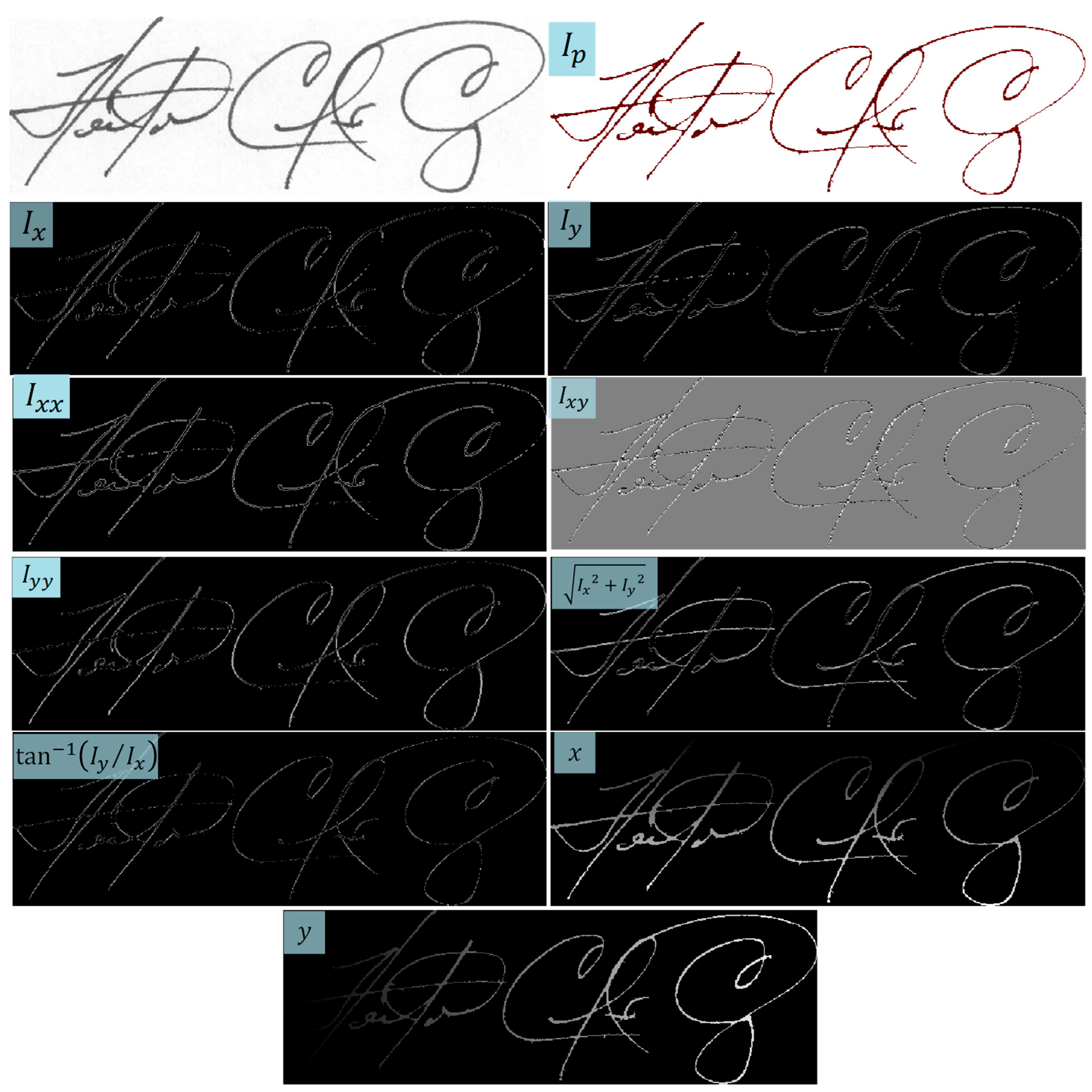
4.2. Signature Image to Covariance Matrix

We briefly review the process that maps an offline signature (i.e., the content of a digital image ${\mathit{I}\mathit{m}\mathit{g}}_{\mathit{X}}$) to its corresponding covariance matrix $\mathit{X}$. The mapping commences by the preprocessing step, which comprises the thresholding and thinning originally proposed in [72] and is then utilized in other research efforts such as [52,55,56]. For each handwritten signature image, the thinning algorithm of [72] detects the optimal thinning level (OTL), a parameter which has been found to affect the verification results of a number of datasets in an optimal way, including the ones that are currently employed [37]. Therefore, the $I_p$ image, i.e., the result of the preprocessing stage, is derived by employing the individual OTL at the thinning stage, and then the corresponding covariance matrix $\mathit{X}$ is extracted accordingly.

A feature map of ten (i.e., $d=10)$ image planes derived from ${\mathit{I}\mathit{m}\mathit{g}}_{\mathit{X}}$ comprises the corresponding image filters$,\left[I_p,I_x,I_y,I_{xx},I_{xy},I_{yy},\sqrt{{I_x}^2+{I_y}^2,}{\tan }^{-1}\left(I_y/I_x\right),x_{,}{y}_{,}\right]$, in which $I_p$ is the result of the preprocessing stage of the ${\mathit{I}\mathit{m}\mathit{g}}_{\mathit{X}}$; $I_x,I_y,I_{xx},I_{xy},I_{yy}$ are the first- and second-order derivatives of $I_p$; $x_{,}{y}_{,}$ are the normalized coordinates (by their maximum number of rows and columns of the image bounding box) of the signature pixels; and $\sqrt{(\cdot )}$ and ${\mathrm{t}\mathrm{a}\mathrm{n}}^{-1}(\cdot )$ denote the gradient magnitude and direction (normalized in radians). The corresponding covariance matrix $\mathit{X}\in {\mathit{P}}_{10}$ is evaluated only on the pixels that belong to the signature trace of the thinning preprocessing step. In the unlikely case that $\mathit{X}$ is not strictly SPD, an additional regularization term, ${10}^{-4}{\mathit{I}}_{10}$, where ${\mathit{I}}_{10}$ is the identity matrix, is added to $\mathit{X}$ in order to ensure it; i.e., $\mathit{X}\leftarrow \mathit{X}+{10}^{-4}\times {\mathit{I}}_{10}$. Figure 5 presents the visual output of the preprocessing stage ($I_p$) along with the outputs produced by the applied filters.

Regarding the use of specific image filters, we report the following: We tried to utilize other types of image filters on the $I_p$ image that have been suggested in the literature for other image recognition and computer vision applications. For example, we created and experimented with covariance matrices that utilize the following:

• A family of Gabor filters in different directions and frequencies.
• A family of difference of Gaussians (DoG).

In addition, we applied a tactic in which for each signature pixel a 5 × 5 window creates a 25-dimensional intensity feature. However, the currently exploited 10 dimensional filters (also utilized in our previous research work) strongly suggest that this is a robust image filter set for signature verification. Most likely, this is due to the nature of the signature, as it is made from handmade strokes depicted as sparse image lines of variable durations and curvature (p. 2, [56]).

4.3. The Learning Framework

The structure of the experimental WI-SV framework draws its inspiration mainly from the seminal work of Rivard et al. [28], which highlights the use of blind, or disjoint, subsets for the development and testing of the model or verifier. It adheres to the underlying assumption that the learning, or development, subset $\mathbb{L}$ of writers used for building and validating the model is sufficient for the testing or exploitation stage. Therefore, in accordance with the Section 1, we make use of two blind sets: (a) the learning set $\mathbb{L}$ and (b) the testing set $\mathbb{T}\mathbb{S}$. The origin of the $\mathbb{L}$ and $\mathbb{T}\mathbb{S}$ sets depends on the intra-lingual or inter-lingual nature of the experimental framework. In the case of the intra-lingual framework, denoted hereafter with ${\mathcal{F}}_{intra}$, any signature dataset ${\mathcal{D}}_i$ splits its initial population of writers into two equally populated subsets, $\mathbb{L}$ and $\mathbb{T}\mathbb{S}$. During one fold, the learning set $\mathbb{L}$ is further divided into the training ${\mathbb{T}}_{\mathbb{R}}$ and validation sets $\mathbb{V}$ so that $\mathbb{L}=\{{\mathbb{T}}_{\mathbb{R}}\cup \mathbb{V}\}$. In the course of the training stage, the ${\mathbb{T}}_{\mathbb{R}}$ set is employed for evaluation of the current operating parameters of the model under learning, while the validation set $\mathbb{V}$ is employed in order to select the optimal operating parameters of the model. In the course of the testing stage, the $\mathbb{T}\mathbb{S}$ subset is employed in order to evaluate the efficiency of the model. Then, in order to conclude the fold, the $\mathbb{L}$ and $\mathbb{T}\mathbb{S}$ subsets swap roles so that the model learns the new $\mathbb{L}\leftarrow \mathbb{T}\mathbb{S}$ and $\mathbb{T}\mathbb{S}\leftarrow \mathbb{L}$. We randomly repeat the selection of the $\mathbb{L},\mathbb{T}\mathbb{S}$ writers five times; this is the so-called $5\times 2$ fold, which has been followed in our experiments [37,55,56]. As for the case of the inter-lingual framework, denoted hereafter with ${\mathcal{F}}_{inter}$, a kind of a transfer learning concept in which the model learns an entire dataset ${\mathcal{D}}_i$, it is then tested over the remaining datasets ${\mathcal{D}}_j, j\ne i$.

We now provide details regarding the generation of the learning set $\mathbb{L}=\{{\mathbb{T}}_{\mathbb{R}}\cup \mathbb{V}\}$. Therefore, let us denote the cardinality of writers for each dataset ${\mathcal{D}}_i$ with ${\mathbb{N}}_{{\mathcal{D}}_i}=\left|{\mathcal{D}}_i\right|$. At each ${\mathcal{F}}_{intra}$ fold, the cardinality of the learning set $\mathbb{L}$ is ${\mathbb{N}}_{\mathbb{L}}=⌈\left|{\mathcal{D}}_i\right|/2⌉$. Each one of the ${\mathbb{N}}_{\mathbb{L}}$ writers is populated by ${\mathbb{N}}_{\mathbb{G}}$ and ${\mathbb{N}}_{\mathcal{S}\mathbb{F}}$ genuine and skilled forgery samples. The ${\mathbb{T}}_{\mathbb{R}}$ and $\mathbb{V}$ subsets are formed by representatives of both the similar and the dissimilar ${\omega }_{{\mathbb{T}}_{\mathbb{R}}}^{\pm }$, ${\omega }_{\mathbb{V}}^{\pm }$ classes. To do so, ${\mathbb{N}}_{\mathbb{G}{\mathbb{T}}_{\mathbb{R}}}=⌈{0.7\mathbb{N}}_{\mathbb{G}}⌉$ and ${\mathbb{N}}_{\mathcal{S}\mathbb{F}{\mathbb{T}}_{\mathbb{R}}}=⌈{0.7\mathbb{N}}_{\mathcal{S}\mathbb{F}}⌉$ samples were reserved for the ${\mathbb{T}}_{\mathbb{R}}$ subset, and ${\mathbb{N}}_{\mathbb{G}\mathbb{V}}=⌊{0.3\mathbb{N}}_{\mathbb{G}}⌋$ and ${\mathbb{N}}_{\mathcal{S}\mathbb{F}\mathbb{V}}=⌊{0.3\mathbb{N}}_{\mathcal{S}\mathbb{F}}⌋$ were reserved for the $\mathbb{V}$ subset. Similar signature pairs from the ${\mathbb{N}}_{\mathbb{G}{\mathbb{T}}_{\mathbb{R}}}$ and ${\mathbb{N}}_{\mathbb{G}\mathbb{V}}$ reserved samples are paired in order to form the G-G representatives of the ${\omega }_{{\mathbb{T}}_{\mathbb{R}}}^{+}$ and ${\omega }_{\mathbb{V}}^{+}$ subsets. As stated earlier, due to the disjoint nature of the followed WI-SV experimental protocol, the formation of the dissimilar G-F pairs as representatives of the ${\omega }_{{\mathbb{T}}_{\mathbb{R}}}^{-}$ and ${\omega }_{\mathbb{V}}^{-}$ classes can be of different kinds. In the case that the second part of the dissimilar pair (F) belongs to random forgeries, then the negative class is formed by G-RF pairs, and we create the ${\omega }_{{\mathbb{T}}_{\mathbb{R}}}^{-100\%RF}$ and ${\omega }_{\mathbb{V}}^{-100\%RF}$ classes.

In the case that the second part of the dissimilar pair (F) belongs to skilled forgeries, then the negative class is formed by G-SF pairs, and we create the ${\omega }_{{\mathbb{T}}_{\mathbb{R}}}^{-0\%RF}$ and ${\omega }_{\mathbb{V}}^{-0\%RF}$ classes. It is obvious that we can generate numerous mixtures for the dissimilar populations with the use of one mixing parameter; however, in this work we will use only the aforementioned setups. Given the significantly larger amount of the negative representatives and the need for balanced sized inputs to the training stage of the classifier, the cardinalities $\left|{\omega }_{{\mathbb{T}}_{\mathbb{R}}}^{-}\right|$, $\left|{\omega }_{\mathbb{V}}^{-}\right|$ of the dissimilar sets $\left|{\omega }_{{\mathbb{T}}_{\mathbb{R}}}^{-0\%RF}\right|$, $\left|{\omega }_{{\mathbb{T}}_{\mathbb{R}}}^{-100\%RF}\right|$, $\left|{\omega }_{\mathbb{V}}^{-0\%RF}\right|$, $\left|{\omega }_{\mathbb{V}}^{-100\%RF}\right|$ were set equal to the $\left|{\omega }_{{\mathbb{T}}_{\mathbb{R}}}^{+}\right|$, $\left|{\omega }_{\mathbb{V}}^{+}\right|$ cardinalities by random selection. Table 2 summarizes all the necessary details. An analogous approach is followed for the ${\mathcal{F}}_{intra}$ cross-lingual protocol. The only thing that changes is that there is no need for a $5\times 2$ fold since now the entire $N_{D_i}$ population is used for creating the ${\omega }^{+}=\{{\omega }_{{\mathbb{T}}_{\mathbb{R}}}^{+},{\omega }_{\mathbb{V}}^{+}\}$ and ${\omega }^{-}=\left\{{\omega }^{-100\%RF}\right\} (or {\omega }^{-0\%RF})$ class-conditioned pairs.

In summary, during the learning stage, the input to the classifier module consists of the similar and dissimilar signature pairs denoted by ${\omega }^{+}=\{{\omega }_{{\mathbb{T}}_{\mathbb{R}}}^{+},{\omega }_{\mathbb{V}}^{+}\}$ and ${\omega }^{-}=\{{\omega }_{{\mathbb{T}}_{\mathbb{R}}}^{-100\%RF},{\omega }_{\mathbb{V}}^{-100\%RF}\}$ or ${\omega }^{-}=\{{\omega }_{{\mathbb{T}}_{\mathbb{R}}}^{-0\%RF},{\omega }_{\mathbb{V}}^{-0\%RF}\}$. For each${\omega }^{+}$, ${\omega }^{-}$ pairs and each $a$-segment, the RDV’s ${\Psi }_{\{g,S,J\}}^a$, ${\Psi }_{\{g,S,J\}}^{\mathit{I},a}$ along with their vectored forms $v_{\{g,S,J\}}^{a\pm }$ and ${dv}_{\{g,S,J\}}^{a\pm }$, are evaluated with the use of either the AIRM, Stein, or Jeffrey measures of Equations (2), (4), and (5) and Table 1.

4.4. The Models—Verifiers

Two popular binary classifiers, a hard-margin SVM and a Gentle Ada Boost Boosting Feature Selection algorithm (BFS), along with a Decision Stump Committee (DSC-BFS) [28,37,73,74], were employed in order to independently build the WI signature verifier. Detailed operation of both the SVM and the DSC-BFS classifiers for both WD and WI signature verification can be found in the literature [28,37,75]. Both models operate under a similar training–validation protocol which will identify their optimal operating parameters. Algorithms 1 and 2 provide an overview of the basic functionality during the learning stage by means of two standard algorithms. In summary, sets of $v_{\{g,S,J\}}^{\pm }$ or ${dv}_{\{g,S,J\}}^{\pm }$ vectors, which correspond to the training set ${\mathbb{T}}_{\mathbb{R}}:{\omega }_{{\mathbb{T}}_{\mathbb{R}}}^{+}$ and ${\omega }_{{\mathbb{T}}_{\mathbb{R}}}^{-100\%RF}$ (or ${\omega }_{{\mathbb{T}}_{\mathbb{R}}}^{-0\%RF}$), are fed to the classifiers, followed by the model training stage. Then, the validation set $\mathbb{V}:{\omega }_{\mathbb{V}}^{+}$ and ${\omega }_{\mathbb{V}}^{-100\%RF}$ (or ${\omega }_{\mathbb{V}}^{-0\%RF}$) in terms of the related $v_{\{g,S,J\}}^{\pm }$ or ${dv}_{\{g,S,J\}}^{\pm }$ is enabled for evaluation of the associated scores ${s\_v}_{\{g,S,J\}}^{\pm }$ (or ${s\_dv}_{\{g,S,J\}}^{\pm }$) returned by the models. The optimal operating parameters are the ones that are associated with the maximum value of the Area under the Curve (AUC), a property of the Receiver Operating Characteristic (ROC) curve [76] of the ${s\_v}_{\{g,S,J\}}^{\pm }$ (or ${s\_dv}_{\{g,S,J\}}^{\pm }$), evaluated only with the validation set $\mathbb{V}$.

The Learning Stage: the basic algorithms—SVM (Algorithm 1) and DSC-BFS (Algorithm 2).

Algorithm 1: Learning a WI-SV verifier with the SVM.

Requires: The ${\omega }^{+}=\{{\omega }_{{\mathbb{T}}_{\mathbb{R}}}^{+},{\omega }_{\mathbb{V}}^{+}\}$ and ${\omega }^{-}=\{{\omega }_{{\mathbb{T}}_{\mathbb{R}}}^{-},{\omega }_{\mathbb{V}}^{-}\}$ by means of $v^{\pm }$ or $d{v}^{\pm }$ Returns: SVM model ${∆}_{SVM}(C_{opt}$, ${\gamma }_{opt})$ with the optimal parameters for hard margin $C_{opt}$ and kernel scale ${\gamma }_{opt}$ BEGIN 1: FOR: A grid search on $C$, $\gamma$ 2: USE: ${\omega }_{{\mathbb{T}}_{\mathbb{R}}}^{+}, {\omega }_{{\mathbb{T}}_{\mathbb{R}}}^{-}$ by means of their vectored forms: $v_{{\mathbb{T}}_{\mathbb{R}}}^{\pm }$ or $d{v}_{{\mathbb{T}}_{\mathbb{R}}}^{\pm }$ 3: TRAIN: The current model ${∆}_{SVM}(C$,$\gamma )$ with $v_{{\mathbb{T}}_{\mathbb{R}}}^{\pm }$ or $d{v}_{{\mathbb{T}}_{\mathbb{R}}}^{\pm }$ 4: USE: ${\omega }_{\mathbb{V}}^{+}, {\omega }_{\mathbb{V}}^{-}$ by means of their vectored forms: $v_{\mathbb{V}}^{\pm }$ or $d{v}_{\mathbb{V}}^{\pm }$ 5: EVAL: Scores ${s\_v}_{\mathbb{V}}^{\pm }$ or ${s\_dv}_{\mathbb{V}}^{\pm }$ with current ${∆}_{SVM}(C$,$\gamma ,v_{\mathbb{V}}^{\pm })$ 6: PERFORM: ROC analysis with ${s\_v}_{\mathbb{V}}^{\pm }$ or ${s\_dv}_{\mathbb{V}}^{\pm }$. 7: EVAL: $AUC(C$,$\gamma )$ from ROC analysis 8: end_FOR 9: RETURN: ${∆}_{SVM}(C_{opt}$, ${\gamma }_{opt})$ which corresponds to the $max\left(AUC\right)$. END

Algorithm 2: Learning a WI-SV verifier with the DSC-BFS.

Requires: The ${\omega }^{+}=\{{\omega }_{{\mathbb{T}}_{\mathbb{R}}}^{+},{\omega }_{\mathbb{V}}^{+}\}$ and ${\omega }^{-}=\{{\omega }_{{\mathbb{T}}_{\mathbb{R}}}^{-},{\omega }_{\mathbb{V}}^{-}\}$ by means of $v^{\pm }$ (or $d{v}^{\pm }$) Returns: DSC-BFS model ${∆}_{\mathrm{D}\mathrm{S}\mathrm{C}-\mathrm{B}\mathrm{F}\mathrm{S}}\left(T_{opt}\right)=sign\left[{\sum }_{t=1}^{T_{opt}}{f}_t\left(v^{\pm }\right)\right]$ with $T_{opt}$ the optimal number of leafs. SET:$T_H$: The early stopping criterion. $T_L$: Maximum number of iterations. SET:${AUC}_{max} \leftarrow -\infty$ BEGIN 1: FOR: $t=1:T_L$ /* Add a new $t$- leaf /* 2:  /* Gentle AdaBoost algorithm */ 3: USE: ${\omega }_{{\mathbb{T}}_{\mathbb{R}}}^{+}, {\omega }_{{\mathbb{T}}_{\mathbb{R}}}^{-}$ by means of their vectored forms: $v_{{\mathbb{T}}_{\mathbb{R}}}^{\pm }$ (or $d{v}_{{\mathbb{T}}_{\mathbb{R}}}^{\pm }$) 4: TRAIN: The current model ${∆}_{\mathrm{D}\mathrm{S}\mathrm{C}-\mathrm{B}\mathrm{F}\mathrm{S}}\left(t\right)$ with $v_{{\mathbb{T}}_{\mathbb{R}}}^{\pm }$ (or $d{v}_{{\mathbb{T}}_{\mathbb{R}}}^{\pm }$) 5: USE: ${\omega }_{\mathbb{V}}^{+}, {\omega }_{\mathbb{V}}^{-}$ by means of their vectored forms: $v_{\mathbb{V}}^{\pm }$ (or $d{v}_{\mathbb{V}}^{\pm }$) 6: EVAL: Scores ${s\_v}_{\mathbb{V}}^{\pm }$ (or ${s\_dv}_{\mathbb{V}}^{\pm }$) with current model ${∆}_{\mathrm{D}\mathrm{S}\mathrm{C}-\mathrm{B}\mathrm{F}\mathrm{S}}(t,v_{\mathbb{V}}^{\pm })$ 7: PERFORM: ROC analysis with ${s\_v}_{\mathbb{V}}^{\pm }$ or ${s\_dv}_{\mathbb{V}}^{\pm }$. 8: EVAL: $AU{C}_t$ from ROC analysis 9: IF $AU{C}_t>{AUC}_{max}$ then 10:  SET: ${AUC}_{max}=AU{C}_t$ 11:  SET: $T_{opt}\leftarrow t$ 12:  SET: counter = 0. 13: ELSE 14:  $counter$ $\leftarrow$ $counter$+1 15:  IF counter ==$T_H$ then 16:   EXIT by early stopping 17:  end_IF 18: end_IF 19: end_FOR 20: RETURN: ${∆}_{\mathrm{D}\mathrm{S}\mathrm{C}-\mathrm{B}\mathrm{F}\mathrm{S}}\left(T_{opt}\right)$ which corresponds to the ${AUC}_{max}$ END

The dimensionality of the input $v_{\{g,S,J\}}^{a\pm }$ and ${dv}_{\{g,S,J\}}^{a\pm } a=1:14$ vectors over all the $a-$ indexed equimass segments is conditioned on the two learning procedures, LFW1 and LFW2 (depicted in Figure 3 and Figure 4 earlier introduced in Section 2.2). In the case of LFW1 visually depicted in Figure 3, the dimensionality of the inputs $v_{\{g,S,J\}}^{a\pm }$ and ${dv}_{\{g,S,J\}}^{a\pm }$ equals fifty-five, as Equation (13) implies for $d=10$. In the case of LFW2, visually depicted in Figure 4, the fused input vector is formed by concatenating all vectors $v_{\{g,S,J\}}^{a\pm }$ or ${dv}_{\{g,S,J\}}^{a\pm }$, resulting in an input dimensionality equal to $14\times 55=770$.

4.5. Description of the Testing Protocol

The returned, now-fixed model verifiers ${∆}_{SVM}$ (or ${∆}_{DSC-BFS}$) are now utilized at the testing stage. For each writer of the testing set $\mathbb{T}\mathbb{S}$, a reference set ${\mathbb{N}}_{REF}$ of $\left|{\mathbb{N}}_{REF}\right|=10$ signature samples is reserved out of its ${\mathbb{N}}_{\mathbb{G}}$ genuine samples. The remaining ${\mathbb{Q}}^{+}=\{{\mathbb{N}}_{\mathbb{G}}-{\mathbb{N}}_{REF}\}$ and ${\mathbb{Q}}^{-}={\mathbb{N}}_{\mathcal{S}\mathbb{F}}$ samples form the $\left|{\mathbb{Q}}^{+}\right|$ positive and $\left|{\mathbb{Q}}^{-}\right|$ negative members of the questioned set ${\mathbb{Q}}^{\pm }=\{{\mathbb{Q}}^{+},{\mathbb{Q}}^{-}\}$. Typically, the ${\mathbb{N}}_{REF}$, ${\mathbb{Q}}^{\pm }$ corresponding covariance matrices are now paired in order to create the RDV’s ${\Psi }_{\{g,S,J\}}^a$ and ${\Psi }_{\{g,S,J\}}^{\mathit{I},a}$, along with their vectored forms $v_{\{g,S,J\}}^{a\pm }$ and ${dv}_{\{g,S,J\}}^{a\pm }$, $a=1:14$. Since we have two learning procedures, the serial LFW1 and the parallel LFW2, we also now provide details regarding their equivalent testing companion, namely the serial TFW1 and the parallel TFW2.

The implementation steps of TFW1 are graphically depicted in Figure 6. For a single covariance pair, $\mathcal{R}\in {\mathbb{N}}_{REF}$ and $\mathit{Q}\in {\mathbb{Q}}^{\pm }$, we begin by evaluating a vector of 14 scores ${sc}_{\mathsf{\Delta }}=\{{sc}_{\mathsf{\Delta }}\left(a\right)\leftarrow {\mathsf{\Delta }}_a\}\in {\mathbb{R}}^{14}$ each with $a$-component ${\mathsf{\Delta }}_a$, $a=1:14$ to correspond to the local spatial segments of Figure 2. Then, the following steps are applied:

• Sort ${sc}_{\mathsf{\Delta }}$ in a descending order, thus creating the $s{c}_{s\mathsf{\Delta }}=\{{sc}_{s\mathsf{\Delta }}\left(a\right)\equiv {s\mathsf{\Delta }}_a\}\in {\mathbb{R}}^{14}$ score vector.
• Generate the final score vector ${sc}_{s\mathsf{\Delta }}^f\in {\mathbb{R}}^{14}$ by (a) assigning its first component ${sc}_{s\Delta }^f\left(1\right)$ to the original ${\mathsf{\Delta }}_1$ value and (b) assigning its value as ${sc}_{s\mathsf{\Delta }}^f\left(a\right)\equiv \overline{{s\mathsf{\Delta }}_a}=\mathit{mean}s{c}_{s\mathsf{\Delta }}\left(1:a\right) \mathrm{f}\mathrm{o}\mathrm{r} \mathrm{e}\mathrm{v}\mathrm{e}\mathrm{r}\mathrm{y} a=1:14 \mathrm{l}\mathrm{o}\mathrm{c}\mathrm{a}\mathrm{l} \mathrm{s}\mathrm{e}\mathrm{g}\mathrm{m}\mathrm{e}\mathrm{n}\mathrm{t}.$

Then, for all $\left|{\mathbb{N}}_{REF}\right|\times \left|{\mathbb{Q}}^{\pm }\right|$ pairs, a stack $D=\left\{D_a\right\}, a=1:14, D_a\in {\mathbb{R}}^{{\left|\mathbb{Q}\right|}^{\pm }\times \left|{\mathbb{N}}_{REF}\right|}$ is formed in which the “$D_a$-level” has elements, which are the corresponding $\overline{{s\mathsf{\Delta }}_a}(\mathcal{R},\mathit{Q})$ values. In conclusion, a final score vector $FSV\left(a\right|{\mathbb{Q}}^{\pm })\in {\mathbb{R}}^{\left|{\mathbb{Q}}^{\pm }\right|}$ is derived by assigning the maximum distance of $\mathit{Q}$ over the entire reference set ${\mathbb{N}}_{REF}$. The $FSV\left(a\right)$ scores are a function of the segment parameter $a$ and are conditioned on the positive or/and negative class. Following the evaluation of the $FSV\left(a\right|{\mathbb{Q}}^{\pm })$ scores, a sliding threshold evaluates the per-writer false acceptance rates ${FAR}_{SF}$ (i.e., skilled forgeries that have been accepted as genuine), the false rejection rates $FRR$ (i.e., genuine samples that have been rejected as forgery), and the corresponding equal error rates ${EER}_{SF}^{user}$ as the point in which ${FAR}_{SF}=FRR$. The above process is repeated ten times for each writer, and the averages are reported as a function of the $a$ parameter in the following section.

The implementation steps of TFW2 are much simpler. Following the learning stage of the ${∆}_{SVM}$ (or ${∆}_{DSC-BFS}$) verifiers with the 770-dimensional feature vectors $\left\{v_{\{g,S,J\}}^{a\pm }\right\}$, $\left\{{dv}_{\{g,S,J\}}^{a\pm }\right\}$ depicted in Figure 4, we utilize the same $\mathbb{T}\mathbb{S}$ set of the TFW1 framework by means of the same reference ${\mathbb{N}}_{REF}$ and questioned ${\mathbb{Q}}^{\pm }=\{{\mathbb{Q}}^{+},{\mathbb{Q}}^{-}\}$ sets. The output of the ${∆}_{SVM}$ (or ${∆}_{DSC-BFS}$) verifiers is a set of scores conditioned on the ${\mathbb{Q}}^{+}$ or ${\mathbb{Q}}^{-}$ classes. In a similar approach, the ${EER}_{SF}^{user}$ is evaluated for each writer. This process is repeated ten times for each writer, and the averages are reported in the succeeding section.

It should be noted that during the implementation of the testing stage (at each repetition) we employ the median optimal thinning level (MOTL) of the reference samples (of each testing writer) so that all images under testing experience the same image preprocessing parameters (by means of the MOTL).

5. Results and Discussion

5.1. ${\mathcal{F}}_{intra}$ Intra-Lingual Experiments

We initiate this section by presenting a thorough evaluation of the proposed inference 5 × 2 intra-lingual fold schemes. From the aforementioned material exposed so far, we have an abundant number of experiment cases, given the fact that there are (a) two kinds of classifiers (SVM, DSC-BSF); (b) two kinds of RDVs, ${\Psi }_{\mathit{{\rm X}},\mathit{Y}}$ (local pole) and ${\Psi }_{\mathit{{\rm X}},\mathit{Y}}^{\mathit{I}}$ (common pole), and corresponding vectors $v_{\mathit{X},\mathit{Y}}$ or ${dv}_{\mathit{X},\mathit{Y}}$; (c) two ways to fuse the $v_{\mathit{X},\mathit{Y}}$ or ${dv}_{\mathit{X},\mathit{Y}}$ vectors and thus create the experimental setups LFW1, TFW1 (serial) and LFW2, TFW12 (parallel); (d) three measures (i.e., AIRM, Stein, Jeffrey) for the creation of the RDVs ${\Psi }_{\mathit{{\rm X}},\mathit{Y}}$ and ${\Psi }_{\mathit{{\rm X}},\mathit{Y}}^{\mathit{I}}$; (e) two ways to form the ${\omega }^{-}$learning set ${\omega }_{{\mathbb{T}}_{\mathbb{R}} or \mathbb{V}}^{-100\%RF}$ (or ${\omega }_{{\mathbb{T}}_{\mathbb{R}}or \mathbb{V}}^{-0\%RF}$); and (f) five datasets. To avoid misperception,

Table 3. Indicative labels used for the ${\mathcal{F}}_{intra}$ experiments.

Design Params.	SPD Measures AIRM, Stein, Jeffrey			${\mathit{\omega }}^{-}$ Formation (100%RF, 0%RF)		$\mathbf{Classifier} \mathbf{Type} ∆$ $\mathit{S}\mathit{V}\mathit{M}$ or DSC-BFS
Label of Experiment	A	S	J	0	100	SVM	DSC-BFS
	Example: Local pole: LFW1
${}_{LFW1}{}^{{\Psi }_{\mathit{{\rm X}},\mathit{Y}}}\mathcal{E}(A,100,SV)$	✓	×	×	×	✓	✓	×
${}_{LFW1}{}^{{\Psi }_{\mathit{{\rm X}},\mathit{Y}}}\mathcal{E}(S,0,DS)$	×	✓	×	✓	×	×	✓
	Example: Common pole: LFW1
${}_{LFW1}{}^{{\Psi }_{\mathit{{\rm X}},\mathit{Y}}^{\mathit{I}}}\mathcal{E}(A,100,SV)$	✓	×	×	×	✓	✓	×
${}_{LFW1}{}^{{\Psi }_{\mathit{{\rm X}},\mathit{Y}}^{\mathit{I}}}\mathcal{E}(S,0,DS)$	×	✓	×	✓	×	×	✓
	Example: Local pole: LFW2
${}_{LFW2}{}^{{\Psi }_{\mathit{{\rm X}},\mathit{Y}}}\mathcal{E}(J,0,DS)$	×	×	✓	✓	×	×	✓
${}_{LFW2}{}^{{\Psi }_{\mathit{{\rm X}},\mathit{Y}}}\mathcal{E}(A,100,SV)$	✓	×	×	×	✓	✓	×
	Example: Common pole: LFW2
${}_{LFW2}{}^{{\Psi }_{\mathit{{\rm X}},\mathit{Y}}^{\mathit{I}}}\mathcal{E}(A,100,SV)$	✓	×	×	×	✓	✓	×
${}_{LFW2}{}^{{\Psi }_{\mathit{{\rm X}},\mathit{Y}}^{\mathit{I}}}\mathcal{E}(S,0,DS)$	×	✓	×	✓	×	×	✓

provides an indicative subset of the labels used in order to characterize the experimental setups. We make use of the subsequent terminology ${}_{Fusio{n}_{kind}}{}^{RD{V}_{kind}}\mathcal{E}(SP{D}_{measure},{\omega }_{way}^{-},∆)$ in order to label the experiments according to the design parameters. For example, ${}_{LFW1}{}^{{\Psi }_{\mathit{{\rm X}},\mathit{Y}}}\mathcal{E}(S,0,SV)$ denotes an experiment with local pole ${\Psi }_{\mathit{{\rm X}},\mathit{Y}}$ RDV, the LFW1/TFW1 protocol, the Stein measure, 0%RF for the ${\omega }^{-}$ formation and the ${\Delta }_{SVM}$ classifier. Therefore, Figure 7, Figure 8, Figure 9, Figure 10 and Figure 11 present the corresponding average ${EER}_{SF}^{user}$ as a function of the segment indexed by $a=1:14$ for the LFW1/TFW1 protocol.

Commenting on the content of Figure 7, Figure 8, Figure 9, Figure 10 and Figure 11, a number of useful comparisons can be deducted regarding the ${EER}_{SF}^{user}$ efficiency with respect to the following design parameters: (a) SVM vs. DSC-BFS, (b) local pole ${\Psi }_{\mathit{{\rm X}},\mathit{Y}}$ vs. common pole ${\Psi }_{\mathit{{\rm X}},\mathit{Y}}^{\mathit{I}}$ RDVs, (c) ${\omega }^{-100\%RF}$ vs. ${\omega }^{-0\%RF}$, and (d) the use of AIRM, Stein, or Jeffrey measure for the formation of the RDVs content.

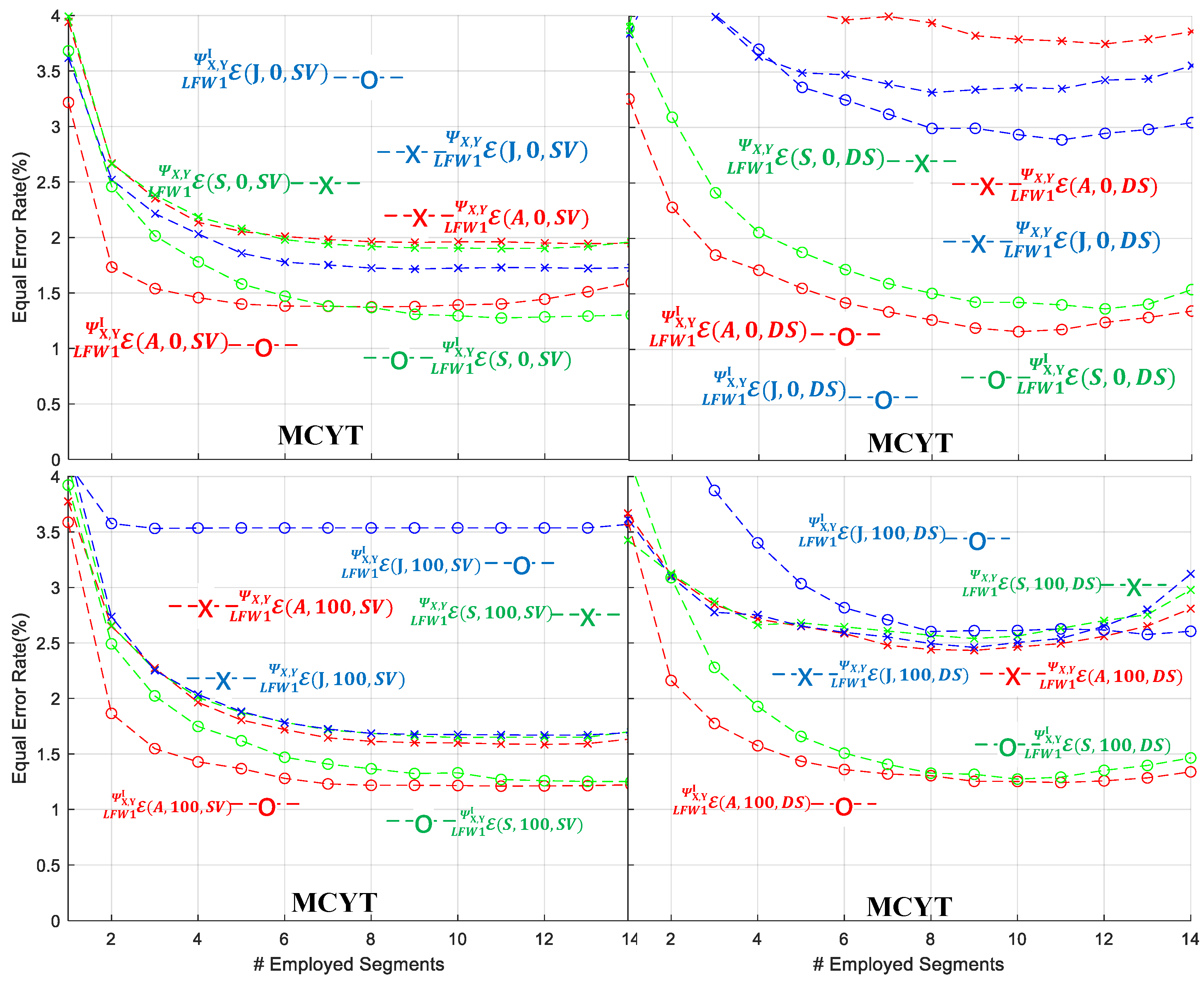
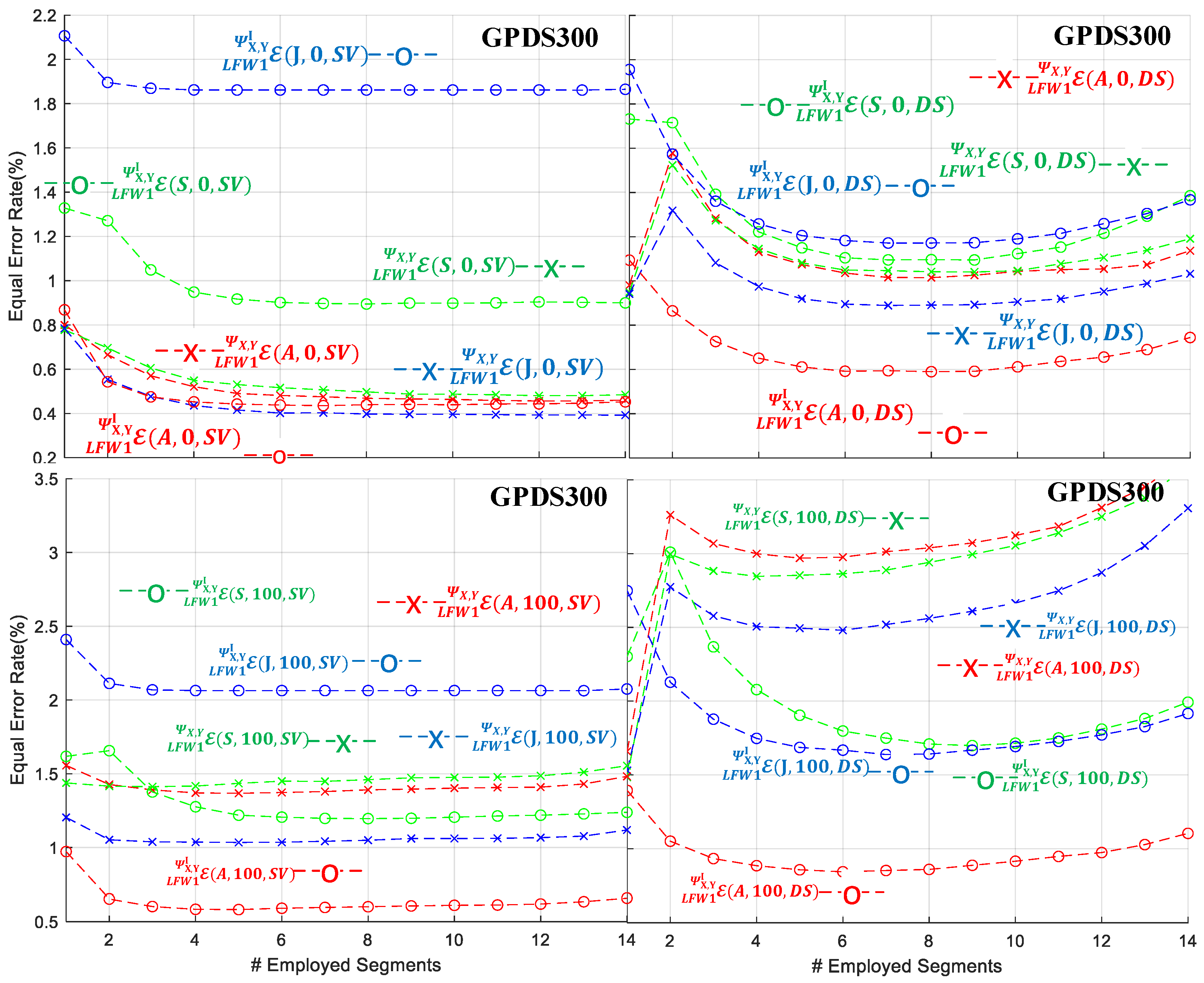
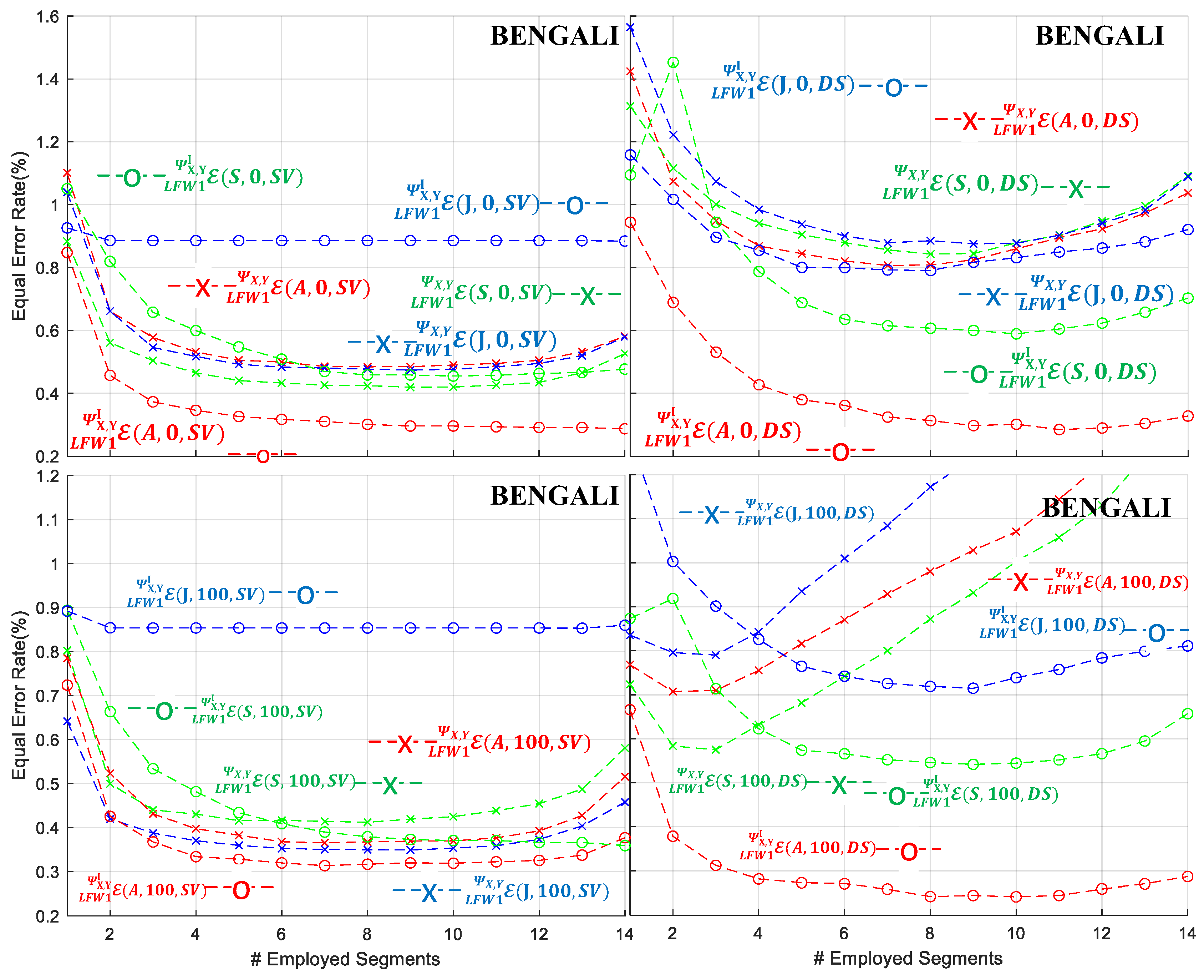
• With respect to the employment of the SVM or the DSC-BFS as the signature verifier, it is evident that all datasets exhibit superior performance under the SVM classifier when compared to the DSC-BFS in terms of average ${EER}_{SF}^{user}$. Furthermore, the SVM module demonstrates higher robustness with respect to SPD measures A, S, and J. This is evidenced by a higher proportion of cases exhibiting lower ${EER}_{SF}^{user}$ results in comparison to the DSC-BFS cases.
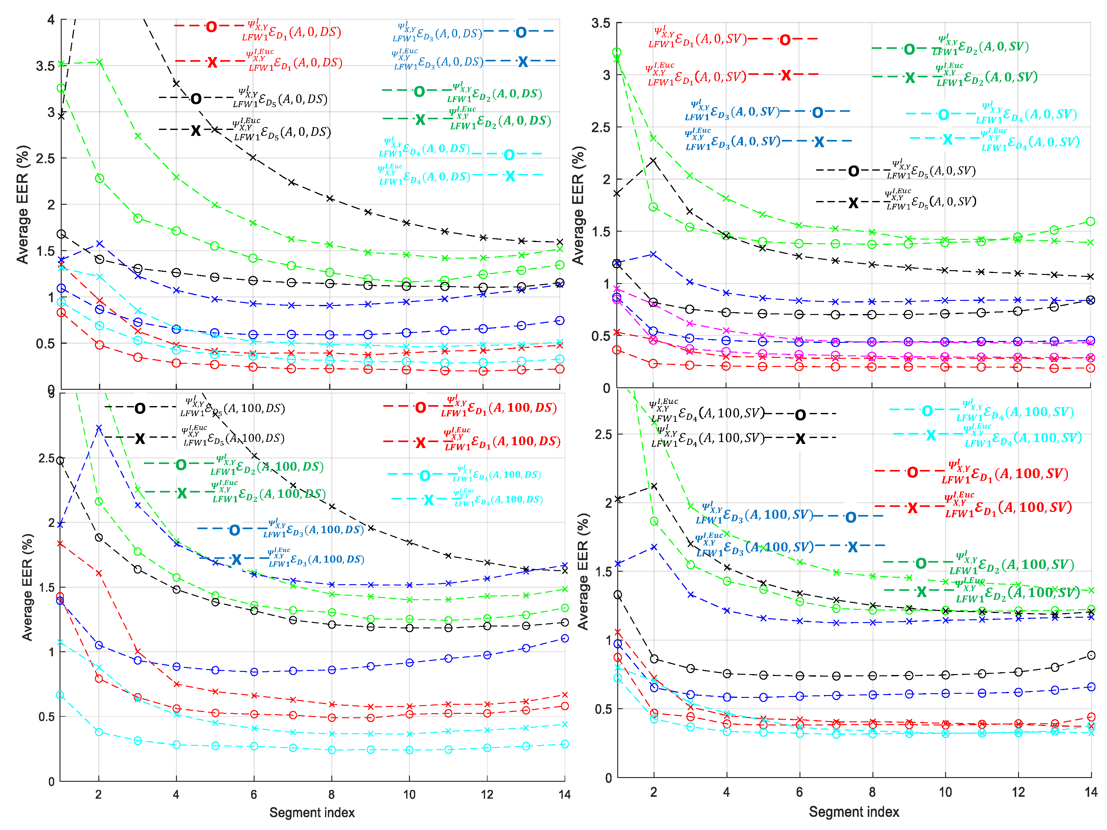
• With respect to the use of the local ${\Psi }_{\mathit{{\rm X}},\mathit{Y}}$ or common pole ${\Psi }_{\mathit{{\rm X}},\mathit{Y}}^{\mathit{I}}$ RDVs highlighted in Figure 7, Figure 8, Figure 9, Figure 10 and Figure 11 it is evident that, with the notable exception of the HINDI dataset, SVM verifier and ${\omega }^{-0\%RF}$, clearly the common pole ${\Psi }_{\mathit{{\rm X}},\mathit{Y}}^{\mathit{I}}$ RDV provides the best average ${EER}_{SF}^{user}$ in all cases. A possible explanation for the higher discriminative capabilities of the common pole ${\Psi }_{\mathit{{\rm X}},\mathit{Y}}^{\mathit{I}}$ RDV approach is that, in the local ${\Psi }_{\mathit{{\rm X}},\mathit{Y}}$ approach, the RDVs are created without having fixed poles, thus making the conditioned class outputs of the ${\left(-\right)}_{\mathcal{M}}$ operator somehow incompatible with each other. Although special care in the form of a parallel transport action could provide a candidate solution, the use of signature images and corresponding covariance matrices that are placed everywhere in the SPD manifold does not allow us to designate a vantage point besides the ${\mathit{I}}_{\mathit{d}}$ already utilized in the ${\Psi }_{\mathit{{\rm X}},\mathit{Y}}^{\mathit{I}}$ RDV.
• With respect to the ${\omega }^{-100\%RF}$ vs. ${\omega }^{-0\%RF}$ negative class formation, it is apparent that for the majority of the cases the ${\omega }^{-0\%RF}$ setup provides the lowest average ${EER}_{SF}^{user}$ rates more robustly. This outcome has been anticipated, given the construction of each individual dataset under similar acquisition and a priori conditions. Consequently, the classifier models learned through the learning procedure with the ${\omega }^{-0\%RF}$ setup of simulated (or skilled) forgery samples inherently exhibit generalization capabilities during the testing stage [55,56].
• With respect to the use of the AIRM, Stein, or Jeffrey measure for the formation of the RVDs, again it is more than evident that, with the notable exception of the HINDI/SVM/${\omega }^{-0\%RF}$, the use of AIRM is more effective compared to the use of the Stein and Jeffrey measures. This should not be considered as a surprise, since the use of AIRM has been reported to optimally operate in a number of cases, including signature verification [56].
• For the case of the LFW2/TFW2 protocol in which a larger 770-dimensional vector is utilized,

  Table 4. ${\mathcal{F}}_{intra}$ and LFW2/TFW2 ${EER}_{SF}^{user}$ (%) for the intra-lingual scheme and the AIRM measure. Minimum values are displayed in bold.

  Experiment Label	Average EER per Signature Dataset
  	CEDAR	MCYT	GPDS300	BANGLA	HINDI
  ${}_{LFW2}{}^{{\Psi }_{\mathit{{\rm X}},\mathit{Y}}}\mathcal{E}(A,0,SV)$	0.278	1.867	1.073	0.383	0.416
  ${}_{LFW2}{}^{{\Psi }_{\mathit{{\rm X}},\mathit{Y}}}\mathcal{E}(A,0,DS)$	0.208	2.094	0.883	0.635	0.811
  ${}_{LFW2}{}^{{\Psi }_{\mathit{{\rm X}},\mathit{Y}}}\mathcal{E}(A,100,SV)$	1.992	2.193	4.183	0.441	1.207
  ${}_{LFW2}{}^{{\Psi }_{\mathit{{\rm X}},\mathit{Y}}}\mathcal{E}(A,100,DS)$	1.240	2.340	2.140	0.543	1.262
  ${}_{LFW2}{}^{{\Psi }_{\mathsf{{\rm X}},\mathbf{Y}}^{\mathbf{I}}}\mathcal{E}(A,0,SV)$	0.206	1.198	0.736	0.353	0.440
  ${}_{LFW2}{}^{{\Psi }_{\mathsf{{\rm X}},\mathbf{Y}}^{\mathbf{I}}}\mathcal{E}(A,0,DS)$	0.261	2.268	1.043	0.473	0.811
  ${}_{LFW2}{}^{{\Psi }_{\mathsf{{\rm X}},\mathbf{Y}}^{\mathbf{I}}}\mathcal{E}(A,100,SV)$	0.385	1.563	1.096	0.241	0.632
  ${}_{LFW2}{}^{{\Psi }_{\mathsf{{\rm X}},\mathbf{Y}}^{\mathbf{I}}}\mathcal{E}(A,100,DS)$	0.799	2.165	1.484	0.459	1.307
  	Common pole—LFW1, a = 8
  ${}_{LFW1}{}^{{\Psi }_{\mathsf{{\rm X}},\mathbf{Y}}^{\mathbf{I}}}\mathcal{E}(A,0,SV)$	0.199	1.368	0.439	0.301	0.466
  ${}_{LFW1}{}^{{\Psi }_{\mathsf{{\rm X}},\mathbf{Y}}^{\mathbf{I}}}\mathcal{E}(A,0,DS)$	0.224	1.264	0.589	0.313	1.144
  ${}_{LFW1}{}^{{\Psi }_{\mathsf{{\rm X}},\mathbf{Y}}^{\mathbf{I}}}\mathcal{E}(A,100,SV)$	0.384	1.217	0.601	0.316	0.739
  ${}_{LFW1}{}^{{\Psi }_{\mathsf{{\rm X}},\mathbf{Y}}^{\mathbf{I}}}\mathcal{E}(A,100,DS)$	0.489	1.304	0.859	0.242	1.2096

  ,

  Table 5. ${\mathcal{F}}_{intra}$ and LFW2/TFW2 ${EER}_{SF}^{user}$ (%) for the intra-lingual scheme and the Stein measure. Minimum values are displayed in bold.

  Experiment Label	Average EER per Signature Dataset
  	CEDAR	MCYT	GPDS300	BANGLA	HINDI
  ${}_{LFW2}{}^{{\Psi }_{\mathit{{\rm X}},\mathit{Y}}}\mathcal{E}(S,0,SV)$	0.295	2.267	1.251	0.838	0.436
  ${}_{LFW2}{}^{{\Psi }_{\mathit{{\rm X}},\mathit{Y}}}\mathcal{E}(S,0,DS)$	0.244	2.052	0.929	1.041	0.779
  ${}_{LFW2}{}^{{\Psi }_{\mathit{{\rm X}},\mathit{Y}}}\mathcal{E}(S,100,SV)$	2.229	2.220	4.698	0.602	1.371
  ${}_{LFW2}{}^{{\Psi }_{\mathit{{\rm X}},\mathit{Y}}}\mathcal{E}(S,100,DS)$	1.376	2.461	2.379	0.676	1.291
  ${}_{LFW2}{}^{{\Psi }_{\mathsf{{\rm X}},\mathbf{Y}}^{\mathbf{I}}}\mathcal{E}(S,0,SV)$	0.466	1.044	1.224	0.602	0.691
  ${}_{LFW2}{}^{{\Psi }_{\mathsf{{\rm X}},\mathbf{Y}}^{\mathbf{I}}}\mathcal{E}(S,0,DS)$	0.635	2.022	1.591	0.720	1.278
  ${}_{LFW2}{}^{{\Psi }_{\mathsf{{\rm X}},\mathbf{Y}}^{\mathbf{I}}}\mathcal{E}(S,100,SV)$	0.618	1.227	1.679	0.447	0.960
  ${}_{LFW2}{}^{{\Psi }_{\mathsf{{\rm X}},\mathbf{Y}}^{\mathbf{I}}}\mathcal{E}(S,100,DS)$	1.393	1.988	2.458	0.642	1.837
  	Common pole—LFW1, a = 8
  ${}_{LFW1}{}^{{\Psi }_{\mathsf{{\rm X}},\mathbf{Y}}^{\mathbf{I}}}\mathcal{E}(S,0,SV)$	0.432	1.368	0.894	0.458	1.047
  ${}_{LFW1}{}^{{\Psi }_{\mathsf{{\rm X}},\mathbf{Y}}^{\mathbf{I}}}\mathcal{E}(S,0,DS)$	0.614	1.504	1.096	0.607	1.752
  ${}_{LFW1}{}^{{\Psi }_{\mathsf{{\rm X}},\mathbf{Y}}^{\mathbf{I}}}\mathcal{E}(S,100,SV)$	0.551	1.368	1.196	0.379	1.127
  ${}_{LFW1}{}^{{\Psi }_{\mathsf{{\rm X}},\mathbf{Y}}^{\mathbf{I}}}\mathcal{E}(S,100,DS)$	0.786	1.326	1.709	0.546	2.137

  and

  Table 6. ${\mathcal{F}}_{intra}$ and LFW2/TFW2 ${EER}_{SF}^{user}$ (%) for the intra-lingual scheme and the Jeffrey measure. Minimum values are displayed in bold.

  Experiment Label	Average EER per Signature Dataset
  	CEDAR	MCYT	GPDS300	BANGLA	HINDI
  ${}_{LFW2}{}^{{\Psi }_{\mathit{{\rm X}},\mathit{Y}}}\mathcal{E}(J,0,SV)$	0.249	2.177	1.362	0.687	0.448
  ${}_{LFW2}{}^{{\Psi }_{\mathit{{\rm X}},\mathit{Y}}}\mathcal{E}(J,0,DS)$	0.225	2.265	1.049	0.964	0.835
  ${}_{LFW2}{}^{{\Psi }_{\mathit{{\rm X}},\mathit{Y}}}\mathcal{E}(J,100,SV)$	2.190	2.170	3.576	0.635	1.472
  ${}_{LFW2}{}^{{\Psi }_{\mathit{{\rm X}},\mathit{Y}}}\mathcal{E}(J,100,DS)$	2.021	2.534	2.290	0.709	1.420
  ${}_{LFW2}{}^{{\Psi }_{\mathsf{{\rm X}},\mathbf{Y}}^{\mathbf{I}}}\mathcal{E}(J,0,SV)$	0.531	3.957	2.108	0.531	0.972
  ${}_{LFW2}{}^{{\Psi }_{\mathsf{{\rm X}},\mathbf{Y}}^{\mathbf{I}}}\mathcal{E}(J,0,DS)$	0.973	4.048	1.800	0.888	1.493
  ${}_{LFW2}{}^{{\Psi }_{\mathsf{{\rm X}},\mathbf{Y}}^{\mathbf{I}}}\mathcal{E}(J,100,SV)$	1.064	2.586	3.444	0.995	1.668
  ${}_{LFW2}{}^{{\Psi }_{\mathsf{{\rm X}},\mathbf{Y}}^{\mathbf{I}}}\mathcal{E}(J,100,DS)$	2.123	3.735	2.671	2.210	2.534
  	Common pole—LFW1, a = 8
  ${}_{LFW1}{}^{{\Psi }_{\mathsf{{\rm X}},\mathbf{Y}}^{\mathbf{I}}}\mathcal{E}(J,0,SV)$	0.864	4.037	1.861	0.885	1.544
  ${}_{LFW1}{}^{{\Psi }_{\mathsf{{\rm X}},\mathbf{Y}}^{\mathbf{I}}}\mathcal{E}(J,0,DS)$	0.846	2.991	1.171	0.790	2.721
  ${}_{LFW1}{}^{{\Psi }_{\mathsf{{\rm X}},\mathbf{Y}}^{\mathbf{I}}}\mathcal{E}(J,100,SV)$	1.115	3.536	2.064	0.853	1.767
  ${}_{LFW1}{}^{{\Psi }_{\mathsf{{\rm X}},\mathbf{Y}}^{\mathbf{I}}}\mathcal{E}(J,100,DS)$	1.775	2.603	1.638	0.718	2.578

  present the corresponding average ${EER}_{SF}^{user}$ error rates. For comparing the results between the serial LFW1 and parallel LFW2 protocols, we complement the contents of Table 4, Table 5 and Table 6 by reporting the optimal LFW1/TFW1 average ${EER}_{SF}^{user}$ as extracted from Figure 7, Figure 8, Figure 9, Figure 10 and Figure 11 for the ${}_{LFW1}{}^{{\Psi }_{\mathit{{\rm X}},\mathit{Y}}^{\mathit{I}}}\mathcal{E}(A,(0 or 100),SV)$ cases and for the $a=8$ segment index to ensure fairness and robustness through all datasets.

A comprehensive examination of Table 4, Table 5 and Table 6 reveals that the use of the AIRM measure, in conjunction with a binary SVM classifier, robustly yields low verification error rates when benchmarked against Stein, Jeffrey’s measure, and the DSC-BFS classifier.

5.2. ${\mathcal{F}}_{inter}$ Cross-Lingual Experiments

Motivated by the results in the previous section and to further avoid another round of excessive experiments, we limited the ${\mathcal{F}}_{inter}$ cross-lingual protocol by using only the AIRM measure. On the other hand, we choose to keep and test both the SVM and DSC-BFS classifiers, as well as the ${\Psi }_{\mathit{{\rm X}},\mathit{Y}}$, ${\Psi }_{\mathit{{\rm X}},\mathit{Y}}^{\mathit{I}}$ RDVs and the ${\omega }^{-100\%RF}$, ${\omega }^{-0\%RF}$ setups accompanied by the LFW1 or LFW2 protocols. Figure 12 presents the average ${EER}_{SF}^{user}$ for the LFW1 protocol in which we learn the verifiers with one dataset $D_i$ and test it over the entire writers of a blind testing set $D_{j\ne i}$. Focusing on the content of Figure 12, we can draw a number of comments regarding EER efficiency with respect to the following design parameters of the local LFW1 protocol: (a) SVM vs. DSC-BFS, (b) local pole ${\Psi }_{\mathit{{\rm X}},\mathit{Y}}$ vs. common pole ${\Psi }_{\mathit{{\rm X}},\mathit{Y}}^{\mathit{I}}$ RDVs, and (c) ${\omega }^{-100\%RF}$ vs. ${\omega }^{-0\%RF}$ setup.

• With respect to the employment of the SVM against the DSC-BFS, the results indicate that the two forms of classifiers demonstrate comparable performance levels, exhibiting marginal disparities in their operational capabilities.
• With respect to the local ${\Psi }_{\mathit{{\rm X}},\mathit{Y}}$ or common pole ${\Psi }_{\mathit{{\rm X}},\mathit{Y}}^{\mathit{I}}$ RDVs, it is again evident that clearly the common pole ${\Psi }_{\mathit{{\rm X}},\mathit{Y}}^{\mathit{I}}$ RDV provides the best average ${EER}_{SF}^{user}$ in the majority of the cases.
• With respect to the ${\omega }^{-100\%RF}$ vs. ${\omega }^{-0\%RF}$ negative class formation, an enhancement in the verification performance of the learned verifiers is observed for the ${\mathsf{\omega }}^{-100\mathrm{\%}\mathrm{R}\mathrm{F}}$ when compared to the ${\omega }^{-0\%RF}.$ Thus, contrary to the elevated verification leverage of the ${\omega }^{-0\%RF}$ on the $F_{intra}$ cases, the development of the classifiers under the ${\mathsf{\omega }}^{-100\mathrm{\%}\mathrm{R}\mathrm{F}}$ assumption on the $F_{inter}$ cases yields more robust models.

Again, for the case of the ${\mathcal{F}}_{inter}$ and the LFW2/TFW2 protocol, in which a larger 770-dimensional vector is utilized,

Table 7. Average ${EER}_{SF}^{user}$ (%) for LFW2, SVM, DSC-BFS, ${\Psi }_{\mathit{{\rm X}},\mathit{Y}}^{\mathit{I}}$, ${\omega }^{-0\mathrm{\%}RF}$, and AIRM. A direct comparison against $LFW1$ cases is also provided. Minimum values are displayed in bold.

${\mathit{E}\mathit{E}\mathit{R}}_{\mathit{S}\mathit{F}}^{\mathit{u}\mathit{s}\mathit{e}\mathit{r}}$	Testing Dataset
	CEDAR		MCYT		GPDS300		BENGALI		HINDI
Learning Dataset	SVM	DSC	SVM	DSC	SVM	DSC	SVM	DSC	SVM	DSC
CEDAR	-		6.49	6.07	1.02	0.95	2.15	1.93	3.87	3.65
MCYT	1.38	2.58	-		3.68	6.06	0.34	0.50	1.16	1.36
GPDS300	0.47	0.44	2.69	2.63	-		1.67	1.32	3.25	3.45
BENGALI	49.9	50.0	49.9	50.0	50.0	50.0	-		1.26	1.44
HINDI	2.04	2.87	2.86	2.82	3.31	4.74	0.80	0.89	-
Comparison against	${}_{LFW1}{}^{{\Psi }_{\mathsf{{\rm X}},\mathbf{Y}}^{\mathbf{I}}}\mathcal{E}\left(A,0,SV\right)\&{}_{LFW1}{}^{{\Psi }_{\mathsf{{\rm X}},\mathbf{Y}}^{\mathbf{I}}}\mathcal{E}\left(A,0,DS\right),a=8$,
CEDAR	-		1.18	1.26	0.47	0.42	0.41	0.43	1.04	1.20
MCYT	0.66	0.70	-		0.93	0.96	0.43	0.47	1.50	1.87
GPDS300	0.28	0.25	1.41	1.36	-		0.47	0.48	1.34	1.61
BENGALI	27.4	37.8	28.4	41.1	0.70	0.78	-		0.90	1.24
HINDI	0.54	0.59	1.38	1.63	1.36	1.47	0.28	0.50	-

and

Table 8. Average ${EER}_{SF}^{user}$ (%) for LFW2, SVM, DSC-BFS, ${\Psi }_{\mathit{{\rm X}},\mathit{Y}}^{\mathit{I}}$, ${\omega }^{-100\mathrm{\%}RF}$, and AIRM. A direct comparison against $LFW1$ cases is also provided. Minimum values are displayed in bold.

${\mathit{E}\mathit{E}\mathit{R}}_{\mathit{S}\mathit{F}}^{\mathit{u}\mathit{s}\mathit{e}\mathit{r}}$	Testing Dataset
	CEDAR		MCYT		GPDS300		BENGALI		HINDI
Learning Dataset	SVM	DSC	SVM	DSC	SVM	DSC	SVM	DSC	SVM	DSC
CEDAR	-		1.92	2.20	1.11	1.14	0.45	0.47	1.27	1.38
MCYT	0.71	0.90	-		1.32	1.51	0.45	0.50	1.24	1.47
GPDS300	0.56	0.60	2.12	2.21	-		0.84	0.72	1.45	1.52
BENGALI	49.9	50.0	49.9	50.0	50.0	50.0	-		0.71	0.85
HINDI	2.16	2.83	2.78	2.73	3.56	4.93	0.64	0.95	-
Comparison against	${}_{LFW1}{}^{{\Psi }_{\mathsf{{\rm X}},\mathbf{Y}}^{\mathbf{I}}}\mathcal{E}\left(A,100,SV\right)\&{}_{LFW1}{}^{{\Psi }_{\mathsf{{\rm X}},\mathbf{Y}}^{\mathbf{I}}}\mathcal{E}\left(A,100,DS\right),a=8$
CEDAR	-		1.18	1.18	0.49	0.53	0.46	0.39	1.18	1.03
MCYT	0.49	0.53	-		0.71	0.71	0.32	0.36	1.26	1.50
GPDS300	0.34	0.30	1.17	1.12	-		0.38	0.30	0.99	1.15
BENGALI	17.2	26.7	18.6	28.2	1.05	1.05	-		0.81	1.01
HINDI	0.75	0.75	2.11	2.39	1.37	1.37	0.24	0.40	-

present the corresponding average ${EER}_{SF}^{user}$ error rates. Again, in order to compare the derived results between the serial LFW1 and parallel LFW2 fusion protocols, we complement their content by reporting the optimal LFW1/TFW1 average ${EER}_{SF}^{user}$ extracted out of Figure 12 for the common pole ${\Psi }_{\mathit{{\rm X}},\mathit{Y}}^{\mathit{I}}$ RDV approach, the SVM classifier, and the $a=8$ segment index to ensure fairness and robustness through all datasets and the ${\mathcal{F}}_{intra}$ protocol. A comparative inspection of the results indicates that the LFW1/TFW1 serial protocol has superior (i.e., lower) verification error rates when compared to the parallel LFW2/TFW2 one. Moreover, by inspection of Figure 12 it is also evident that the verification error rates can drop much more for the local LFW1/TFW1 protocol for higher values of the segment index $a>8$.

As Figure 12 and Table 7 and Table 8 illustrate, the poor verification performance exhibited by both classifiers when the BENGALI and HINDI datasets are employed for learning purposes is discernible. Specifically, the BENGALI and HINDI subsets demonstrate suboptimal performance when their learned verifier models are evaluated against the CEDAR, MCYT, and GPDS300 dataset. This deficiency in the performance can be attributed to the fact that the Bengali and Hindi SPD points are derived from corresponding binary images, which consequently gives rise to covariance matrices with their first line and column equal to zero, apart from the first variance, which is set to one. On the other hand, this is not observed when the verifiers learn from gray-scale signatures emerging from the CEDAR, MCYT, and GPDS300 datasets. Therefore, it can be inferred that higher generalization necessitates the utilization of gray-scale images in lieu of binary images.

In summary, we provide the following assertions:

• The common pole RDV ${\Psi }_{\mathit{{\rm X}},\mathit{Y}}^{\mathit{I}}$ accompanied by the local LFW1/TFW1 protocol provides lower verification error rates.
• For the case of testing signatures emerging from fixed a priori acquisition conditions and signature styles (e.g., Western, Asian) as in the $F_{intra}$ protocol, the use of the ${\omega }^{-0\%RF}$ seems to be more efficient. On the other hand, in the case of having unknown a priori acquisition conditions and signature styles as in the $F_{inter}$ protocol, the use of the ${\omega }^{-100\%RF}$seems to be more efficient.
• For the $F_{inter}$ protocol and the local LFW1/TFW1, efficiency seems to be an increasing function of segment index $a$. As an example, the MCYT dataset achieves ${EER}_{SF}^{user}$ lower than 1% when the segment index $a$ has greater values than eight (8). For the $F_{intra}$ protocol, such efficient behavior is not observed. This aggregation of scores, as a function of the segment index $a$, can be intuitively seen as the attempt of a computer vision system to incorporate the knowledge of the most similar parts of the signature pairs in a qualitative and quantitative way. Therefore, the incorporation of a large number of segments can be useful in cases of testing pairs of signatures for which we do not have any ground truth regarding their acquisition conditions or origins. In the case that this kind of ground truth is known, then a moderate selection of segment scores provides the optimal verification error rates.

5.3. Comparisons with Euclidean Representations

We conclude the present analysis with a discussion of a key question. Specifically, we inquire as to whether the efficacy of the Euclidean representation systematically underperforms compared to that of the geometrically constrained approach. To address this, we repeated our experiments for all datasets and the $F_{intra}$, ${\omega }^{-0\%RF}$,${\omega }^{-100\%RF}$ experimental protocols and the common pole approach. But in this case, the ${\Psi }_{\mathit{{\rm X}},\mathit{Y}}^{\mathit{I},Euc}$ Euclidean difference vector formation lacks the geometrical constraints of the SPD manifold, so the Euclidean-based ${\Psi }_{\mathit{{\rm X}},\mathit{Y}}^{\mathit{I},Euc}$ DV is provided simply by the vector space matrix subtraction along with the Dichotomy Transform, which is eventually reduced to the following:

$${\Psi }_{\mathit{{\rm X}},\mathit{Y}}^{\mathit{I},Euc}=\left|\left(\mathit{I}-\mathit{X}\right)-\left(\mathit{I}-\mathit{Y}\right)\right|=\left|\mathit{Y}-\mathit{X}\right|=\left|\mathit{X}-\mathit{Y}\right|$$

(14)

followed by a corresponding $ve{c}_{euc}(\cdot )$ vector operator of Equation (13), which finally provides local $v_{Euc}$ representation.

Figure 13 directly compares, in terms of the average ${EER}_{SF}^{user}$, the verification efficiency of the corresponding SPD and Euclidean vector space experiments. The performance of the SPD approach is indisputably superior to the Euclidean one with a minor exception of the $D_2$ (MCYT) dataset, at the ${}_{LFW1}\mathcal{E}_{D_2}(A,100,SV)$ experiment, and for values of the segment index greater than twelve ($a\ge 12$). This systematically observed advantage of considering data in the SPD manifold compared to the hitherto view of them as elements of a vector space can be evidence for assuming SPD representations in the form of covariance matrices as a flexible image representation tactic capable of blending multiple image modalities while compactly capturing their second-order statistics.

Finally, the performance of the proposed approach is compared to the existing literature. To this end, both direct results (i.e., experiments were performed by the authors) along with a comparative summary are presented in

Table 9. Direct comparisons (DCs, denoted with ✓) and comparative summary of WI-SV systems. Performance metrics are either the average (per user and dataset) equal error rate ${EER}_{SF}^{user}$ or the average (per user and dataset) error rate ${AvE}_{SF}^{user}$. The number in the parentheses denotes the number of reference samples during the testing stage.

Method and [Ref] and DC (✓)	Metric	$\mathbf{Datasets} \mathbf{and} (\left|{\mathbb{N}}_{\mathit{R}\mathit{E}\mathit{F}}\right|$)
		CEDAR	MCYT	GPDS300	BANGLA	HINDI
Graph edit distance (MCS) [77]	${EER}_{SF}^{user}$	5.91(10)	3.91(10)
Surroundedness [78]	${EER}_{SF}^{user}$	8.33(1)	-	13.7(1)	-	-
Region Deep Metric (MSDN) [79]	${EER}_{SF}^{user}$	1.75(10) 1.67(12)	-	-	-	-
Point2Set DML [80]	${EER}_{SF}^{user}$	5.22(5)	9.86(5)	-	-	-
DMML(with HOG) [81]	${EER}_{SF}^{user}$	-	13.4(5) and 9.86(10)	-	-	-
Partially ordered sets [37] ✓	${EER}_{SF}^{user}$	2.90(5)	3.50(5)	3.06(5)
DCCM and Feat. Diss. Thresh. [82]	${AvE}_{SF}^{user}$	2.10(5)	-	18.4(5)	-	-
SURDS [35]	${AvE}_{SF}^{user}$	-	-	-	12.6(8)	10.5(8)
TransOSV [19]	${EER}_{SF}^{user}$	-	-	-	9.90(1) 3.56(1)	3.24(1)
Sim. Dist. Learn. (SPD) [55] ✓ $F_{intra}$ 100%RF, a = 4 (${\mathcal{D}}_1$) or a = 7 (${\mathcal{D}}_{\mathrm{2,4},5}$)	${EER}_{SF}^{user}$	0.37(10)	0.96(10)	-	0.26(10)	0.77(10)
Sim. Dist. Learn. (SPD) [55] ✓ $F_{intra}$ 0%RF, a = 4 (${\mathcal{D}}_1$) or a = 7 (${\mathcal{D}}_{\mathrm{2,4},5}$)	${EER}_{SF}^{user}$	0.38(10)	1.02(10)	-	0.25(10)	0.78(10)
ESC-DPDF [29]	${AvE}_{SF}^{user}$	-	-	17.8(12)	-	-
Siamese Network and CCA [83]	${EER}_{SF}^{user}$	3.31(12)	-	-	-	-
HTCSigNet [23]	${EER}_{SF}^{user}$	-	-	-	8.52(12)	4.63(12)
[30] ${CNN SVM}_{max}$ and (IH)	${EER}_{SF}^{user}$	3.32(12)	2.89(10)	3.47(12)	-	-
Sigmml and ERP (SPD) [56] ✓ $F_{intra}$ 0%RF, a = 1 (${\mathcal{D}}_{\mathrm{1,2},\mathrm{4,5}}$)	${EER}_{SF}^{user}$	0.04(10)	0.03(10)	-	0.19(10)	0.17(10)
Proposed (SPD), $F_{intra}$, a = 8, ${}_{LFW1}{}^{{\Psi }_{\mathsf{{\rm X}},\mathrm{Y}}^{\mathrm{I}}}\mathcal{E}(A,100,SV)$	${EER}_{SF}^{user}$	0.38(10)	1.22(10)	0.60(10)	0.32(10)	0.74(10)
Proposed (SPD), $F_{intra}$, a = 8, ${}_{LFW1}{}^{{\Psi }_{\mathsf{{\rm X}},\mathrm{Y}}^{\mathrm{I}}}\mathcal{E}(A,0,SV)$	${EER}_{SF}^{user}$	0.20(10)	1.37(10)	0.44(10)	0.30(10)	0.47(10)

. We choose to report only WI-SV cases that clearly and explicitly stated the number of reference samples ($\left|{\mathbb{N}}_{REF}\right|$) during the implementation of the testing stage. The inspection of the contents of Table 9 is quite interesting. They strongly indicate that modeling the handwritten signature images as entities that lie into matrix manifolds yields low verification error rates, which can be considered competent for other state-of-the-art, data-driven approaches.

6. Conclusions

This work introduces, for the first time, a framework for writer-independent signature verification, which leverages Riemannian dissimilarity vectors (RDVs) on Symmetric Positive Definite Manifolds. The proposed approach involves the extension of the popular Dichotomy Transform to the Riemannian framework. This extension effectively models the geometric properties of signature data within matrix manifolds, thereby improving verification efficiency. The experimental results on multiple datasets, encompassing both intra- and cross-lingual scenarios, substantiate the method’s resilience and its capacity for generalization. The outcomes demonstrate that the method exhibits performance comparable to that of computationally intensive alternatives. Local and global common pole RDV representations, combined with two fusion strategies, are utilized to tackle key challenges in writer-independent signature verification, such as the limited availability of genuine samples and the varied nature of forgeries. The use of three Riemannian measures (AIRM, Stein, and Jeffrey divergences) offers a valuable contribution to advancing the domain. Future research will explore the use of different manifold geometries to handwritten signature embedding and coding.

References

1. Jain, A.K.; Deb, D.; Engelsma, J.J. Biometrics: Trust, But Verify. IEEE Trans. Biom. Behav. Identity Sci. 2022, 4, 303–323. [Google Scholar] [CrossRef]
2. Dargan, S.; Kumar, M. A comprehensive survey on the biometric recognition systems based on physiological and behavioral modalities. Expert Syst. Appl. 2020, 143, 113114. [Google Scholar] [CrossRef]
3. Hameed, M.M.; Ahmad, R.; Kiah, M.L.M.; Murtaza, G. Machine learning-based offline signature verification systems: A systematic review. Signal Process. Image Commun. 2021, 93, 116139. [Google Scholar] [CrossRef]
4. Deviterne-Lapeyre, M.; Ibrahim, S. Interpol questioned documents review 2019–2022. Forensic Sci. Int. Synerg. 2023, 6, 100300. [Google Scholar] [CrossRef]
5. Singla, A.; Mittal, A. Exploring offline signature verification techniques: A survey based on methods and future directions. Multimed. Tools Appl. 2024, 84, 2835–2875. [Google Scholar] [CrossRef]
6. Diaz, M.; Ferrer, M.A.; Impedovo, D.; Malik, M.I.; Pirlo, G.; Plamondon, R. A Perspective Analysis of Handwritten Signature Technology. ACM Comput. Surv. 2018, 51, 1–39. [Google Scholar] [CrossRef]
7. Engin, D.; Kantarcı, A.; Arslan, S.; Ekenel, H.K. Offline Signature Verification on Real-World Documents. In Proceedings of the IEEE/CVF Conference on Computer Vision and Pattern Recognition Workshops, Seattle, WA, USA, 14–19 June 2020; pp. 3518–3526. [Google Scholar]
8. Bromley, J.; Guyon, I.; LeCun, Y.; Säckinger, E.; Shah, R. Signature verification using a “siamese” time delay neural network. In Proceedings of the Advances in Neural Information Processing Systems (NIPS 1993), Denver, CO, USA, 29 November–2 December 1993. [Google Scholar]
9. Impedovo, D.; Pirlo, G.; Plamondon, R. Handwritten Signature Verification: New Advancements and Open Issues. In Proceedings of the 2012 International Conference on Frontiers in Handwriting Recognition, Bari, Italy, 18–20 September 2012; pp. 367–372. [Google Scholar]
10. Stauffer, M.; Maergner, P.; Fischer, A.; Riesen, K. A Survey of State of the Art Methods Employed in the Offline Signature Verification Process. In New Trends in Business Information Systems and Technology: Digital Innovation and Digital Business Transformation; Springer: Cham, Switzerland, 2021; pp. 17–30. [Google Scholar]
11. Impedovo, D.; Pirlo, G. Automatic signature verification in the mobile cloud scenario: Survey and way ahead. IEEE Trans. Emerg. Top. Comput. 2018, 9, 554–568. [Google Scholar] [CrossRef]
12. Faundez-Zanuy, M.; Fierrez, J.; Ferrer, M.A.; Diaz, M.; Tolosana, R.; Plamondon, R. Handwriting Biometrics: Applications and Future Trends in e-Security and e-Health. Cogn. Comput. 2020, 12, 940–953. [Google Scholar] [CrossRef]
13. Lai, S.; Jin, L.; Zhu, Y.; Li, Z.; Lin, L. SynSig2Vec: Forgery-Free Learning of Dynamic Signature Representations by Sigma Lognormal-Based Synthesis and 1D CNN. IEEE Trans. Pattern Anal. Mach. Intell. 2022, 44, 6472–6485. [Google Scholar] [CrossRef]
14. Okawa, M. Online signature verification using single-template matching with time-series averaging and gradient boosting. Pattern Recognit. 2020, 102, 107227. [Google Scholar] [CrossRef]
15. Vorugunti, C.S.; Guru, D.S.; Mukherjee, P.; Pulabaigari, V. OSVNet: Convolutional Siamese Network for Writer Independent Online Signature Verification. In Proceedings of the 2019 International Conference on Document Analysis and Recognition (ICDAR), Sydney, Australia, 20–25 September 2019; pp. 1470–1475. [Google Scholar]
16. Alpar, O. Online signature verification by continuous wavelet transformation of speed signals. Expert Syst. Appl. 2018, 104, 33–42. [Google Scholar] [CrossRef]
17. Tolosana, R.; Vera-Rodriguez, R.; Ortega-Garcia, J.; Fierrez, J. Preprocessing and Feature Selection for Improved Sensor Interoperability in Online Biometric Signature Verification. IEEE Access 2015, 3, 478–489. [Google Scholar] [CrossRef]
18. Shih, M.-C.; Huang, T.-L.; Shih, Y.-H.; Shuai, H.-H.; Liu, H.-T.; Yeh, Y.-R.; Huang, C.-C. DetailSemNet: Elevating Signature Verification Through Detail-Semantic Integration. In Proceedings of the European Conference on Computer Vision (ECCV), Milan, Italy, 29 September–4 October 2024; Springer: Cham, Switzerland, 2025; pp. 449–466. [Google Scholar]
19. Li, H.; Wei, P.; Ma, Z.; Li, C.; Zheng, N. TransOSV: Offline Signature Verification with Transformers. Pattern Recognit. 2024, 145, 109882. [Google Scholar] [CrossRef]
20. Abosamra, G.; Oqaibi, H. A Signature Recognition Technique with a Powerful Verification Mechanism Based on CNN and PCA. IEEE Access 2024, 12, 40634–40656. [Google Scholar] [CrossRef]
21. Viana, T.B.; Souza, V.L.F.; Oliveira, A.L.I.; Cruz, R.M.O.; Sabourin, R. A multi-task approach for contrastive learning of handwritten signature feature representations. Expert Syst. Appl. 2023, 217, 119589. [Google Scholar] [CrossRef]
22. Thakur, U.; Sharma, A. Offline handwritten mathematical recognition using adversarial learning and transformers. Int. J. Doc. Anal. Recognit. (IJDAR) 2023, 27, 147–158. [Google Scholar] [CrossRef]
23. Zheng, L.; Wu, D.; Xu, S.; Zheng, Y. HTCSigNet: A Hybrid Transformer and Convolution Signature Network for offline signature verification. Pattern Recognit. 2024, 159, 111146. [Google Scholar] [CrossRef]
24. Arab, N.; Nemmour, H.; Chibani, Y. A new synthetic feature generation scheme based on artificial immune systems for robust offline signature verification. Expert Syst. Appl. 2023, 213, 119306. [Google Scholar] [CrossRef]
25. Muhtar, Y.; Muhammat, M.; Yadikar, N.; Aysa, A.; Ubul, K. FC-ResNet: A Multilingual Handwritten Signature Verification Model Using an Improved ResNet with CBAM. Appl. Sci. 2023, 13, 8022. [Google Scholar] [CrossRef]
26. Maruyama, T.M.; Oliveira, L.S.; Britto, A.S.; Sabourin, R. Intrapersonal Parameter Optimization for Offline Handwritten Signature Augmentation. IEEE Trans. Inf. Forensics Secur. 2021, 16, 1335–1350. [Google Scholar] [CrossRef]
27. Diaz, M.; Ferrer, M.A.; Eskander, G.S.; Sabourin, R. Generation of Duplicated Off-Line Signature Images for Verification Systems. IEEE Trans. Pattern Anal. Mach. Intell. 2017, 39, 951–964. [Google Scholar] [CrossRef]
28. Rivard, D.; Granger, E.; Sabourin, R. Multi-feature extraction and selection in writer-independent off-line signature verification. Int. J. Doc. Anal. Recognit. 2013, 16, 83–103. [Google Scholar] [CrossRef]
29. Eskander, G.S.; Sabourin, R.; Granger, E. Hybrid writer-independent writer-dependent offline signature verification system. IET Biom. 2013, 2, 169–181. [Google Scholar] [CrossRef]
30. Souza, V.L.F.; Oliveira, A.L.I.; Cruz, R.M.O.; Sabourin, R. A white-box analysis on the writer-independent dichotomy transformation applied to offline handwritten signature verification. Expert Syst. Appl. 2020, 154, 113397. [Google Scholar] [CrossRef]
31. Longjam, T.; Kisku, D.R.; Gupta, P. Writer independent handwritten signature verification on multi-scripted signatures using hybrid CNN-BiLSTM: A novel approach. Expert Syst. Appl. 2023, 214, 119111. [Google Scholar] [CrossRef]
32. Long, J.; Xie, C.; Gao, Z. High discriminant features for writer-independent online signature verification. Multimed. Tools Appl. 2023, 82, 38447–38465. [Google Scholar] [CrossRef]
33. Bird, J.J.; Naser, A.; Lotfi, A. Writer-independent signature verification; Evaluation of robotic and generative adversarial attacks. Inf. Sci. 2023, 633, 170–181. [Google Scholar] [CrossRef]
34. Manna, S.; Chattopadhyay, S.; Bhattacharya, S.; Pal, U. SWIS: Self-Supervised Representation Learning for Writer Independent Offline Signature Verification. In Proceedings of the 2022 IEEE International Conference on Image Processing (ICIP), Bordeaux, France, 16–19 October 2022; pp. 1411–1415. [Google Scholar]
35. Chattopadhyay, S.; Manna, S.; Bhattacharya, S.; Pal, U. SURDS: Self-Supervised Attention-guided Reconstruction and Dual Triplet Loss for Writer Independent Offline Signature Verification. In Proceedings of the 2022 26th International Conference on Pattern Recognition (ICPR), Montreal, QC, Canada, 21–25 August 2022; pp. 1600–1606. [Google Scholar]
36. Parcham, E.; Ilbeygi, M.; Amini, M. CBCapsNet: A novel writer-independent offline signature verification model using a CNN-based architecture and capsule neural networks. Expert Syst. Appl. 2021, 185, 115649. [Google Scholar] [CrossRef]
37. Zois, E.N.; Alexandridis, A.; Economou, G. Writer independent offline signature verification based on asymmetric pixel relations and unrelated training-testing datasets. Expert Syst. Appl. 2019, 125, 14–32. [Google Scholar] [CrossRef]
38. Galbally, J.; Gomez-Barrero, M.; Ross, A. Accuracy evaluation of handwritten signature verification: Rethinking the random-skilled forgeries dichotomy. In Proceedings of the 2017 IEEE International Joint Conference on Biometrics (IJCB), Denver, CO, USA, 1–4 October 2017; pp. 302–310. [Google Scholar]
39. Santos, C.; Justino, E.J.R.; Bortolozzi, F.; Sabourin, R. An off-line signature verification method based on the questioned document expert’s approach and a neural network classifier. In Proceedings of the Ninth International Workshop on Frontiers in Handwriting Recognition, Kokubunji, Japan, 26–29 October 2004; pp. 498–502. [Google Scholar]
40. Oliveira, L.; Justino, E.; Sabourin, R. Off-line Signature Verification Using Writer-Independent Approach. In Proceedings of the 2007 International Joint Conference on Neural Networks, Orlando, FL, USA, 12–17 August 2007; pp. 2539–2544. [Google Scholar]
41. Bertolini, D.; Oliveira, L.S.; Justino, E.; Sabourin, R. Reducing forgeries in writer-independent off-line signature verification through ensemble of classifiers. Pattern Recognit. 2010, 43, 387–396. [Google Scholar] [CrossRef]
42. Eskander, G.S.; Sabourin, R.; Granger, E. Adaptation of Writer-Independent Systems for Offline Signature Verification. In Proceedings of the 2012 International Conference on Frontiers in Handwriting Recognition, Bari, Italy, 18–20 September 2012; pp. 434–439. [Google Scholar]
43. Ren, J.-X.; Xiong, Y.-J.; Zhan, H.; Huang, B. 2C2S: A two-channel and two-stream transformer based framework for offline signature verification. Eng. Appl. Artif. Intell. 2023, 118, 105639. [Google Scholar] [CrossRef]
44. Lu, X.; Huang, L.; Yin, F. Cut and Compare: End-to-end Offline Signature Verification Network. In Proceedings of the 2020 25th International Conference on Pattern Recognition (ICPR), Milan, Italy, 10–15 January 2021; pp. 3589–3596. [Google Scholar]
45. Wei, P.; Li, H.; Hu, P. Inverse Discriminative Networks for Handwritten Signature Verification. In Proceedings of the IEEE Conference on Computer Vision and Pattern Recognition, Long Beach, CA, USA, 15–20 June 2019; pp. 5764–5772. [Google Scholar]
46. Dey, S.; Dutta, A.; Toledo, J.I.; Ghosh, S.K.; Lladós, J.; Pal, U. SigNet: Convolutional Siamese Network for Writer Independent Offline Signature Verification. arXiv 2017, arXiv:1707.02131. [Google Scholar]
47. Cha, S.-H.; Srihari, S. Writer Identification: Statistical Analysis and Dichotomizer. In Advances in Pattern Recognition; Ferri, F., Iñesta, J., Amin, A., Pudil, P., Eds.; Lecture Notes in Computer Science; Springer: Berlin/Heidelberg, Germany, 2000; Volume 1876, pp. 123–132. [Google Scholar]
48. Pekalska, E.; Duin, R.P.W. Dissimilarity-based classification for vectorial representations. In Proceedings of the 18th International Conference on Pattern Recognition (ICPR’06), Hong Kong, China, 20–24 August 2006; pp. 137–140. [Google Scholar]
49. Pekalska, E.; Duin, R.P.W. Beyond Traditional Kernels: Classification in Two Dissimilarity-Based Representation Spaces. IEEE Trans. Syst. Man Cybern. Part C (Appl. Rev.) 2008, 38, 729–744. [Google Scholar] [CrossRef]
50. Duin, R.W.; Loog, M.; Pȩkalska, E.; Tax, D.J. Feature-Based Dissimilarity Space Classification. In Recognizing Patterns in Signals, Speech, Images and Videos; Ünay, D., Çataltepe, Z., Aksoy, S., Eds.; Lecture Notes in Computer Science; Springer: Berlin/Heidelberg, Germany, 2010; Volume 6388, pp. 46–55. [Google Scholar]
51. Faraki, M.; Harandi, M.T.; Porikli, F. A Comprehensive Look at Coding Techniques on Riemannian Manifolds. IEEE Trans. Neural Netw. Learn. Syst. 2018, 29, 5701–5712. [Google Scholar] [CrossRef] [PubMed]
52. Zois, E.N.; Said, S.; Tsourounis, D.; Alexandridis, A. Subscripto multiplex: A Riemannian symmetric positive definite strategy for offline signature verification. Pattern Recognit. Lett. 2023, 167, 67–74. [Google Scholar] [CrossRef]
53. Giazitzis, A.; Diaz, M.; Zois, E.N.; Ferrer, M.A. Janus-Faced Handwritten Signature Attack: A Clash Between a Handwritten Signature Duplicator and a Writer Independent, Metric Meta-learning Offline Signature Verifier. In Proceedings of the 18th International Conference on Document Analysis and Recognition, Athens, Greece, 30 August–4 September 2024; Springer: Cham, Switzerland, 2024; pp. 216–232. [Google Scholar]
54. Giazitzis, A.; Zois, E.N. SigmML: Metric meta-learning for Writer Independent Offline Signature Verification in the Space of SPD Matrices. In Proceedings of the 2024 IEEE/CVF Winter Conference on Applications of Computer Vision (WACV), Waikoloa, HI, USA, 3–8 January 2024; pp. 6300–6310. [Google Scholar]
55. Zois, E.N.; Tsourounis, D.; Kalivas, D. Similarity Distance Learning on SPD Manifold for Writer Independent Offline Signature Verification. IEEE Trans. Inf. Forensics Secur. 2024, 19, 1342–1356. [Google Scholar] [CrossRef]
56. Giazitzis, A.; Zois, E.N. Metric meta-learning and intrinsic Riemannian embedding for writer independent offline signature verification. Expert Syst. Appl. 2025, 261, 125470. [Google Scholar] [CrossRef]
57. Pennec, X.; Fillard, P.; Ayache, N. A Riemannian Framework for Tensor Computing. Int. J. Comput. Vis. 2006, 66, 41–66. [Google Scholar] [CrossRef]
58. Souza, V.L.F.; Oliveira, A.L.I.; Sabourin, R. A Writer-Independent Approach for Offline Signature Verification using Deep Convolutional Neural Networks Features. In Proceedings of the 2018 7th Brazilian Conference on Intelligent Systems (BRACIS), Sao Paulo, Brazil, 22–25 October 2018; pp. 212–217. [Google Scholar]
59. Kumar, A.; Bhatia, K. Offline Handwritten Signature Verification Using Decision Tree. In Cyber Technologies and Emerging Sciences; Springer: Singapore, 2023; pp. 305–313. [Google Scholar]
60. Huang, Z.; Wang, R.; Li, X.; Liu, W.; Shan, S.; Gool, L.V.; Chen, X. Geometry-Aware Similarity Learning on SPD Manifolds for Visual Recognition. IEEE Trans. Circuits Syst. Video Technol. 2018, 28, 2513–2523. [Google Scholar] [CrossRef]
61. Wang, R.; Wu, X.J.; Chen, Z.; Hu, C.; Kittler, J. SPD Manifold Deep Metric Learning for Image Set Classification. IEEE Trans. Neural Netw. Learn. Syst. 2024, 35, 8924–8938. [Google Scholar] [CrossRef]
62. Sra, S. A new metric on the manifold of kernel matrices with application to matrix geometric means. In Proceedings of the Advances in Neural Information Processing Systems (NIPS), Lake Tahoe, NV, USA, 3–6 December 2012; 25, pp. 1–9. [Google Scholar]
63. Wang, Z.; Vemuri, B.C. An affine invariant tensor dissimilarity measure and its applications to tensor-valued image segmentation. In Proceedings of the 2004 IEEE Computer Society Conference on Computer Vision and Pattern Recognition, Washington, DC, USA, 27 June–2 July 2004; p. I-228-233. [Google Scholar]
64. Faraki, M.; Harandi, M.T.; Porikli, F. More about VLAD: A leap from Euclidean to Riemannian manifolds. In Proceedings of the 2015 IEEE Conference on Computer Vision and Pattern Recognition (CVPR), Boston, MA, USA, 7–12 June 2015; pp. 4951–4960. [Google Scholar]
65. Jégou, H.; Perronnin, F.; Douze, M.; Sánchez, J.; Pérez, P.; Schmid, C. Aggregating Local Image Descriptors into Compact Codes. IEEE Trans. Pattern Anal. Mach. Intell. 2012, 34, 1704–1716. [Google Scholar] [CrossRef]
66. Tuzel, O.; Porikli, F.; Meer, P. Pedestrian Detection via Classification on Riemannian Manifolds. IEEE Trans. Pattern Anal. Mach. Intell. 2008, 30, 1713–1727. [Google Scholar] [CrossRef]
67. Pennec, X. 3—Manifold-valued image processing with SPD matrices. In Riemannian Geometric Statistics in Medical Image Analysis; Pennec, X., Sommer, S., Fletcher, T., Eds.; Academic Press: Cambridge, MA, USA, 2020; pp. 75–134. [Google Scholar]
68. Kalera, M.K.; Srihari, S.; Xu, A. Offline signature verification and identification using distance statistics. Int. J. Pattern Recognit. Artif. Intell. 2004, 18, 1339–1360. [Google Scholar] [CrossRef]
69. Vargas, J.F.; Ferrer, M.A.; Travieso, C.M.; Alonso, J.B. Off-line signature verification based on grey level information using texture features. Pattern Recognit. 2011, 44, 375–385. [Google Scholar] [CrossRef]
70. Ortega-Garcia, J.; Fierrez-Aguilar, J.; Simon, D.; Gonzalez, J.; Faundez-Zanuy, M.; Espinosa, V.; Satue, A.; Hernaez, I.; Igarza, J.J.; Vivaracho, C.; et al. MCYT baseline corpus: A bimodal biometric database. IEE Proc. Vis. Image Signal Process. 2003, 150, 395–401. [Google Scholar] [CrossRef]
71. Pal, S.; Alaei, A.; Pal, U.; Blumenstein, M. Performance of an Off-Line Signature Verification Method Based on Texture Features on a Large Indic-Script Signature Dataset. In Proceedings of the 2016 12th IAPR Workshop on Document Analysis Systems (DAS), Santorini, Greece, 11–14 April 2016; pp. 72–77. [Google Scholar]
72. Zois, E.N.; Tsourounis, D.; Theodorakopoulos, I.; Kesidis, A.L.; Economou, G. A Comprehensive Study of Sparse Representation Techniques for Offline Signature Verification. IEEE Trans. Biom. Behav. Identity Sci. 2019, 1, 68–81. [Google Scholar] [CrossRef]
73. Friedman, J.; Hastie, T.; Tibshirani, R. Additive logistic regression: A statistical view of boosting (with discussion and a rejoinder by the authors). Ann. Stat. 2000, 28, 337–407. [Google Scholar] [CrossRef]
74. Iba, W.; Langley, P. Induction of One-Level Decision Trees. In Machine Learning Proceedings 1992; Sleeman, D., Edwards, P., Eds.; Morgan Kaufmann: San Francisco, CA, USA, 1992; pp. 233–240. [Google Scholar]
75. Zois, E.N.; Alewijnse, L.; Economou, G. Offline signature verification and quality characterization using poset-oriented grid features. Pattern Recognit. 2016, 54, 162–177. [Google Scholar] [CrossRef]
76. Fawcett, T. An introduction to ROC analysis. Pattern Recognit. Lett. 2006, 27, 861–874. [Google Scholar] [CrossRef]
77. Maergner, P.; Pondenkandath, V.; Alberti, M.; Liwicki, M.; Riesen, K.; Ingold, R.; Fischer, A. Combining graph edit distance and triplet networks for offline signature verification. Pattern Recognit. Lett. 2019, 125, 527–533. [Google Scholar] [CrossRef]
78. Kumar, R.; Sharma, J.D.; Chanda, B. Writer-independent off-line signature verification using surroundedness feature. Pattern Recognit. Lett. 2012, 33, 301–308. [Google Scholar] [CrossRef]
79. Liu, L.; Huang, L.; Yin, F.; Chen, Y. Offline signature verification using a region based deep metric learning network. Pattern Recognit. 2021, 118, 108009. [Google Scholar] [CrossRef]
80. Zhu, Y.; Lai, S.; Li, Z.; Jin, L. Point-to-Set Similarity Based Deep Metric Learning for Offline Signature Verification. In Proceedings of the 2020 17th International Conference on Frontiers in Handwriting Recognition (ICFHR), Dortmund, Germany, 8–10 September 2020; pp. 282–287. [Google Scholar]
81. Soleimani, A.; Araabi, B.N.; Fouladi, K. Deep Multitask Metric Learning for Offline Signature Verification. Pattern Recognit. Lett. 2016, 80, 84–90. [Google Scholar] [CrossRef]
82. Hamadene, A.; Chibani, Y. One-Class Writer-Independent Offline Signature Verification Using Feature Dissimilarity Thresholding. IEEE Trans. Inf. Forensics Secur. 2016, 11, 1226–1238. [Google Scholar] [CrossRef]
83. Zheng, L.; Zhao, X.; Xu, S.; Ren, Y.; Zheng, Y. Learning discriminative representations by a Canonical Correlation Analysis-based Siamese Network for offline signature verification. Eng. Appl. Artif. Intell. 2025, 139, 109640. [Google Scholar] [CrossRef]
Figure 1. Toy example of the two concepts of the Riemannian dissimilarity vectors (RDVs) between any two points X , Y ϵ P 10 on the SPD manifold. (a) Local approach: The local Riemannian dissimilarity vector Ψ ϵ R 10 × 10 is a symmetric matrix which lies on the local tangent plane of  X . A v e c ( ) operator transforms the symmetric matrix Ψ to a vectored form v . (b) Global (or common pole) approach: evaluation of Riemannian dissimilarity vectors Ψ I , X and Ψ I , Y with respect to the common pole I 10 followed by the Euclidean-based DT Ψ Χ , Y I = Ψ I , X Ψ I , Y and a v e c ( ) operator resulting in the d v .
Applsci 15 07015 g001
Figure 2. The process of creating an array of SPD covariance matrices (marked with colored pixels) over one static signature image. Equimass segments S i are applied in a 1 × 1 and 2 × 2 and 3 × 3 equimass partition of the original image. Indexing of each sub-image block and corresponding SPP matrices X a , Y a also appear.
Applsci 15 07015 g002
Figure 3. The local fusion strategy LFW1: sets of positive (G-G) and negative (G-RF or G-SF) of the entire image X 1 ± , Y 1 ± covariance matrix pairs form the corresponding v { } 1 ± or d v { } 1 ± . Then, two different classifiers, a binary SVM or a Decision Stump Committee are trained and validated in order to select the optimal parameters of each one. Contrary to Figure 4, the LFW1 learning procedure involves only the entire image X 1 ± , Y 1 ± covariance matrix.
Applsci 15 07015 g003
Figure 4. The parallel fusion strategy LFW2: The learning procedure utilizes a vector with larger dimensionality. It is formed by concatenating all vectors, v { } a ± , d v { } a ± , a = 1:14, over all equimass segments.
Applsci 15 07015 g004
Figure 5. Example of the preprocessing procedure and the applied filters. Top left: the original handwritten signature. Top right: the output of the preprocessing (threshold and thinning). The remaining images depict the visual output of each image filter: I x , I y , I x x , I x y , I y y , I x 2 + I y 2 , tan 1 I y / I x , x , y .
Applsci 15 07015 g005
Figure 6. Depiction of the TFW1 testing protocol. For a pair of signature images, a set of 14 covariance matrices are evaluated and fed as pairs to the trained model verifier in order to evaluate the local scores. Sorting and averaging created a stack of fourteen levels D a R Q ± × N R E F  between all possible pairs Q ± × N R E F . The final vector F S V ( a | Q ± ) R Q ± is evaluated by taking the minimum distance of any Q ± over all N R E F .
Applsci 15 07015 g006
Figure 7. F i n t r a and LFW1 experimental setup: average E E R S F u s e r (%) CEDAR dataset.
Applsci 15 07015 g007
Figure 8. F i n t r a  and LFW1 experimental setup: average E E R S F u s e r (%) MCYT dataset.
Applsci 15 07015 g008
Figure 9. F i n t r a  and LFW1 experimental setup: average E E R S F u s e r (%) GPDS300 dataset.
Applsci 15 07015 g009
Figure 10. F i n t r a and LFW1 experimental setup: average E E R S F u s e r (%) BENGALI dataset.
Applsci 15 07015 g010
Figure 11. F i n t r a and LFW1 experimental setup: average E E R S F u s e r (%) HINDI dataset.
Applsci 15 07015 g011
Figure 12. Average E E R S F u s e r (%) for the F i n t e r and LFW1/TFW1 experimental setup for all datasets. TR denotes the learning dataset D i , while TS denotes all the remaining testing datasets D j i . The AIRM measure is used.
Applsci 15 07015 g012
Figure 13. Direct comparisons, in terms of the average E E R S F u s e r (%), for the Euclidean (EUC) Ψ Χ , Y I , E u c and the SPD Ψ Χ , Y I approach under the 5 × 2 F i n t r a protocol, local LFW1/TFW1, 0%RF, 100%RF, and all D i datasets.
Applsci 15 07015 g013