Article

The Application of Numerical Ductile Fracture Simulation in the LBB Evaluation of Nuclear Pipes

1
Key Laboratory of Impact and Safety Engineering, Ministry of Education, Ningbo University, Ningbo 315211, China
2
School of Mechanical Engineering, Sungkyunkwan University, Seoul 03063, Republic of Korea
*
Author to whom correspondence should be addressed.
Appl. Sci. 2025, 15(13), 7010; https://doi.org/10.3390/app15137010 (registering DOI)
Submission received: 20 May 2025 / Revised: 16 June 2025 / Accepted: 19 June 2025 / Published: 21 June 2025

Abstract

:
The leak-before-break (LBB) concept is widely used in the design and estimation of piping systems of nuclear power plants, which requires considerable test work to obtain the fracture resistance (J-R) curves of nuclear pipes. The application of numerical ductile fracture simulation can effectively limit the test work. In this study, an extended stress-modified critical strain (SMCS) model is applied to simulate the crack growth behaviors of full-scale nuclear pipes (SA312 TP304L stainless steel) with a circumferential through-wall crack under a four-point bending load. The LBB evaluation is performed based on the J-R curves of CT specimens and full-scale pipes obtained from fracture resistance tests and numerical simulations. It shows that due to the high crack-tip constraint effect, CT specimens may cause lots of conservatism in the LBB evaluation of nuclear pipes, while the application of numerical ductile fracture simulation can largely reduce the conservatism.

1. Introduction

Since the 1980s, with the development of elastic–plastic fracture mechanics and experience in nuclear power plant operations, researchers have reached the conclusion that nuclear pipes show a large amount of leakage before breakage. It has also been proven that the leakage can be detected by leakage monitoring systems long before the pipe breaks down, and there will be enough time to fix or replace the cracked pipe; thus, major accidents can be prevented [1,2,3]. The design of nuclear pipes based on this conclusion is called the LBB design concept, in which it is not necessary to consider the dynamic effect due to pipe breaks, and the construction cost can be significantly reduced by eliminating unnecessary pipe whip restraints and jet impingement devices. The application of the LBB design concept needs to determine the critical load level at which a cracked nuclear pipe suddenly breaks down, which requires the J-R curves of cracked pipes.
The J-integral, as a parameter characterizing the energy release rate and a core criterion in elastic–plastic fracture mechanics, is widely used in crack propagation analysis of engineering structures, the fracture toughness evaluation of materials, and structural integrity assessments under complex stress conditions. Unlike the stress intensity factor (K), which is limited to linear elastic fracture mechanics (LEFM), the J-integral extends its applicability to nonlinear material behavior, making it an indispensable tool for evaluating fractures in ductile materials. By quantifying the energy per unit area associated with crack propagation, the J-integral serves as a unified parameter for fracture toughness assessment, fatigue analysis, and failure prediction. Its path independence ensures robustness in numerical simulations and experimental measurements. The material’s ability to resist crack propagation under elastic–plastic conditions can also be expressed using the J-integral, namely the J-R curve.
In practical application, the specimens listed in ASTM E 1820 [4](e.g., CT specimens) are usually used to evaluate the J-R curves of nuclear pipes. Due to the high crack-tip constraint effect in these specimens with a deep crack length dominated by bending load, an LBB evaluation based on these specimens usually causes a lot of conservatism [5]. However, considering the high cost and implementation difficulties of full-scale nuclear pipe testing, two-parameter fracture constraint theories (e.g., J-Q) [6,7,8] have been developed to transform the J-R curves obtained from standard specimens to those of full-scale pipes. These theories can characterize the crack-tip fields and quantify constraint levels for various geometries and loading configurations in elastic–plastic material. However, lots of research shows that these theories lose their validity at large-scale yielding [9,10]. Instead of standard specimens, several nonstandard specimens with a more similar crack-tip constraint to that of full-scale pipes have been developed and can more effectively predict the fracture behaviors of nuclear pipes [11,12]. Nonetheless, lots of test work is still required to obtain the J-R curves, including the development of the specific test methodology and fixtures for nonstandard specimens.
A numerical ductile fracture simulation provides an efficient approach for predicting the J-R curves of nuclear pipes. Many damage models have been developed for FE ductile fracture simulation [13,14]. The widely used damage models can be primarily categorized as continuum damage mechanics (CDM) models or micromechanical damage models. CDM, also referred to as macroscopic damage mechanics, is a phenomenological approach based on continuum mechanics and thermodynamics. CDM employs internal variables to characterize the irreversible evolution of microstructural defects (e.g., microcracks, voids) within materials and also considers the damage process as a dissipative process coupled with plastic deformation, creep, and other mechanisms. Kim et al. [15] adopted Bonora’s damage model based on CDM to predict the stress-state-dependent plastic behavior and fracture of 304L stainless steel. Moattari et al. [16] employed a combined framework of CDM and Beremin models to characterize the two competing failure mechanisms in the ductile-to-brittle transition (DTB) region of ferritic steels and predict the fracture toughness scatter band in relation to temperature. However, it should be noted that CDM does not explicitly account for the microscopic mechanisms governing material fracture.
The micromechanics of damage postulates that material damage evolution originates from the nucleation and propagation of microdefects, including dislocations, slip bands, microvoids, and microcracks, with microvoids and microcracks being the predominant damage forms. As a typical micromechanical damage model, the Gurson–Tvergaard–Needleman (GTN) model [17] effectively simulates ductile fracture through micromechanical processes including void nucleation, growth, and coalescence. Ding et al. [18] primarily investigated the ductile fracture prediction of titanium foil considering size effects based on the shear-modified GTN damage model. Comparisons with experimental results verified the accuracy and feasibility of the model. Min et al. [19] improved the GTN model by introducing an independent shear damage variable along with strain rate hardening, thermal softening, and viscous resistance terms to predict the Taylor impact fracture behavior of 7XXX aluminum alloys under high strain rates. However, the complex parameter system of the improved model increased calibration difficulty. In contrast, the stress-modified critical strain (SMCS) model offers a simplified approach by focusing on void growth and assuming constant stress triaxiality, thereby reducing the number of required parameters and facilitating more efficient material calibration. Oh et al. [20] introduced a finite element damage method based on the SMCS model. By incorporating this model into FE analysis, the initiation and propagation of cracks can be effectively simulated. Jeon et al. [21] extended the SMCS model by introducing a constant to characterize the effect of thermal aging on the multiaxial fracture strain of CF8M stainless steel and further utilized the J-R curve to evaluate the fracture toughness of CF8M. Youn et al. [22] predicted the degradation of the fracture toughness in thermally aged CF8A materials under cyclic loading conditions by applying the SMCS model, i.e., the thermal embrittlement constant. However, FE ductile fracture simulation is more often used to predict the crack growth behaviors of small specimens rather than large components like full-scale pipes [23,24,25,26]. As the FE ductile fracture simulation shows a high dependence on the element size near the crack tip, an element size of less than 0.2 mm is usually required to simulate the crack growth behaviors validly [26,27,28]. The use of such small elements to predict the crack growth behaviors of full-scale pipes may cause numerical problems. Nam et al. [28] effectively reduce the element size dependence by introducing an element-size-dependent critical damage parameter into the SMCS model.
In this study, the extended SMCS model is applied to predict the J-R curves of three full-scale pipes with a circumferential through-wall crack under a four-point-bending load. To demonstrate the validity of FE ductile fracture simulation in the LBB evaluation of nuclear pipes, the critical load levels at which cracked pipes suddenly break down predicted based on the FE simulation results are compared to those predicted based on the fracture resistance test results of CT specimens and full-scale pipes.

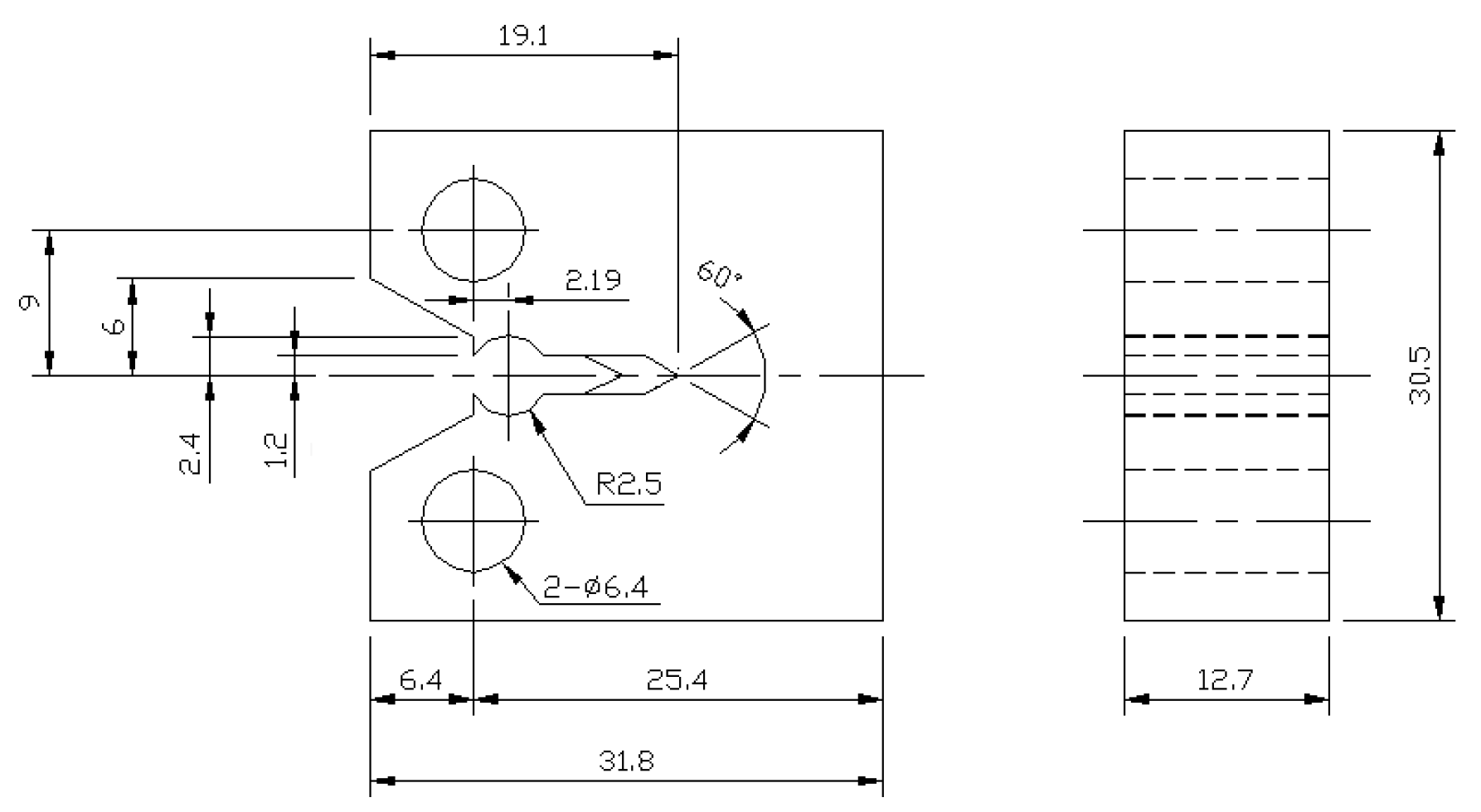
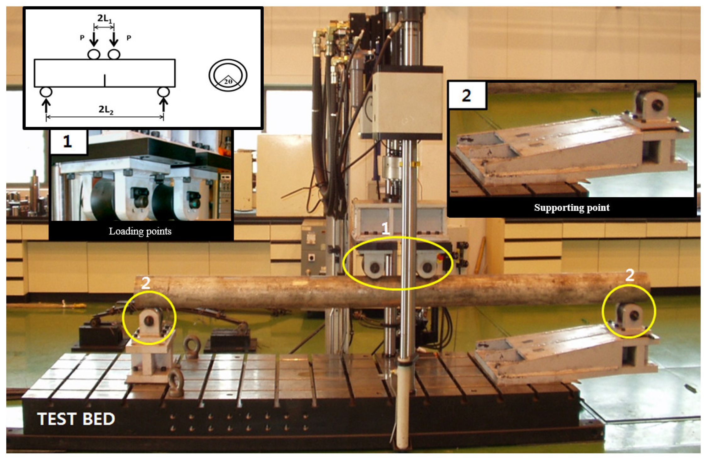
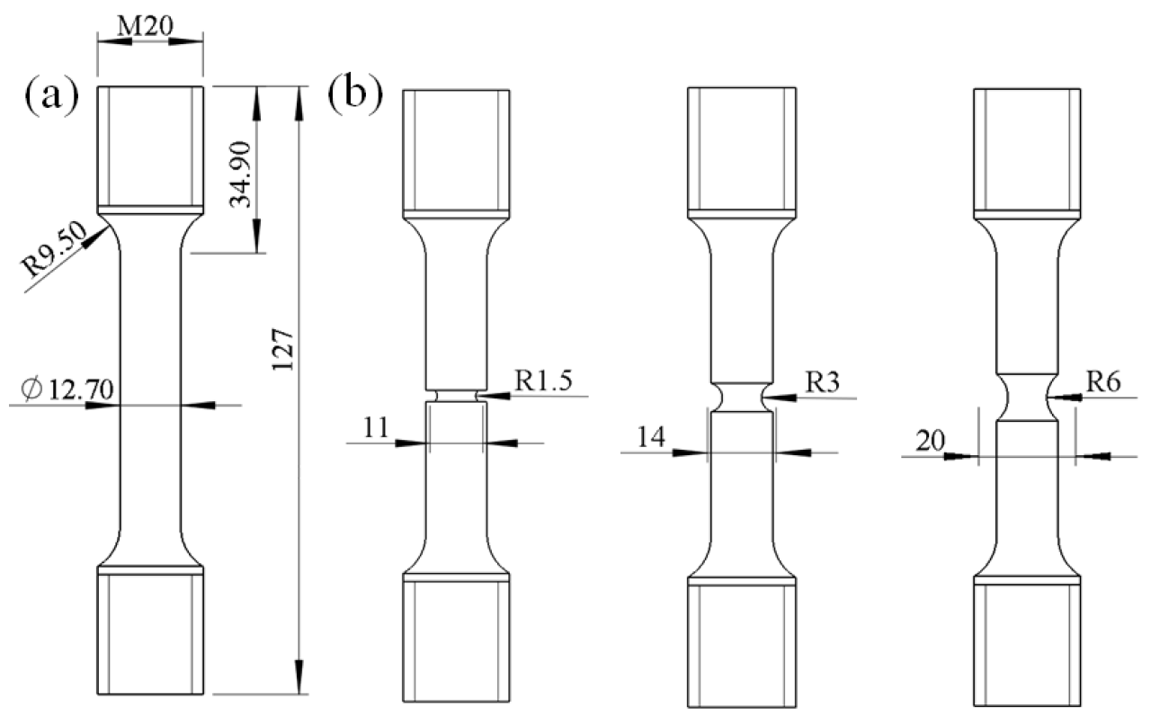
2. Materials and Methods

Due to its excellent corrosion resistance, good weldability, low-carbon design, and outstanding mechanical properties, SA312 TP304L stainless steel has been widely used for heat transport piping in nuclear power plants. Fracture resistance tests conducted on CT specimens and full-scale pipes to evaluate the J-R curves of TP304L pipes with a mean diameter of 168 mm and thickness of 18 mm were introduced in detail in our previous studies [29]. Figure 1 shows the geometry of a 0.5T-CT specimen, which was precracked to a/W = 0.55 with a 10% side groove on both sides. The J-R curves of CT specimens were obtained following the procedure listed in ASTM E 1820 [4], as shown in Figure 2.
The loading condition in full-scale pipe tests is shown in Figure 3, with the inner loading span (2L1) of 300 mm and the outer loading span (2L2) of 2800 mm. The pipes were precracked under fatigue load to 2θ = 60°, 120°, and 180°. Figure 4 shows the full-scale pipe test results. The J-R curves were calculated according to the equations given by Zahoor and Kanninen [29,30], in which the J-integral is determined by superposing the elastic term Je and the plastic term Jp as follows:
J = J e + J p
The elastic term Je can be derived from the elastic solution of the GE/EPRI J-estimation scheme handbook as follows:
J e = R ¯ 2 π a F ^ 2 a b , R ¯ t M 2 E I 2
where R ¯ is the mean pipe radius, t is the pipe wall thickness, a is the half crack length, b = π R ¯ , E is the elastic modulus, I is the second moment of area, M is the bending moment, and F ^ is the geometry function of the elastic stress intensity factor.
The elastic term Jp can be obtained by
J p = 2 0 δ p [ η β P ] d δ p + 2 R ¯ a 0 a γ β J p d a
η β = 2 P L A 1 P L
γ β = 2 P L / a 2 P L / a
where δ p is the plastic displacement, P is half of the total applied load in a four-point bend test, a 0   is the initial half crack length, β is the half crack angle, η and γ are the factors obtained from the first and second derivatives of the function with respect to β , and P L is the limit load.

3. Numerical Ductile Fracture Simulation

3.1. Ductile Fracture Model

In this study, the SMCS model, which simplifies the microvoid damage evolution process and assumes that critical fracture strain ( ε f ) is only related to the stress triaxiality ( σ m / σ e , the ratio of mean normal stress and equivalent stress), is applied to simulate the crack growth behavior of SA312 TP304L stainless steel pipes:
ε f = A   e x p 1.5 σ m σ e + B
where A and B are material constants, which can be determined by fitting the test data of smooth and notched bars. The accumulated damage is calculated as
ω = Δ ω = Δ ε p ε f
where Δ ε p is the equivalent plastic strain increment. Usually, when the accumulated damage becomes unity, ω = ∑Δω = 1, ductile failure is assumed. However, as crack-tip stress and strain in FE simulation show high dependence on the element size, to achieve valid simulation results, an element size of less than 0.2 mm is usually required, which will lead to numerical problems in the simulation of crack growth behaviors for full-scale pipes. Thus, an element-size-dependent critical damage parameter (ωc) is introduced, which ensures a larger element size can be used in the simulation. The value of ωc for specific element size can be calibrated by comparing the simulation and test results of CT specimens. When the damage value of an element reaches ωc, the stress in the element is reduced sharply (a decrease of 5000 MPa) to a small plateau value (10 MPa), then the Young’s modulus is decreased to 100 MPa to keep the numerical stability. The SMCS model is implemented in ABAQUS 6.14 through the user subroutines.

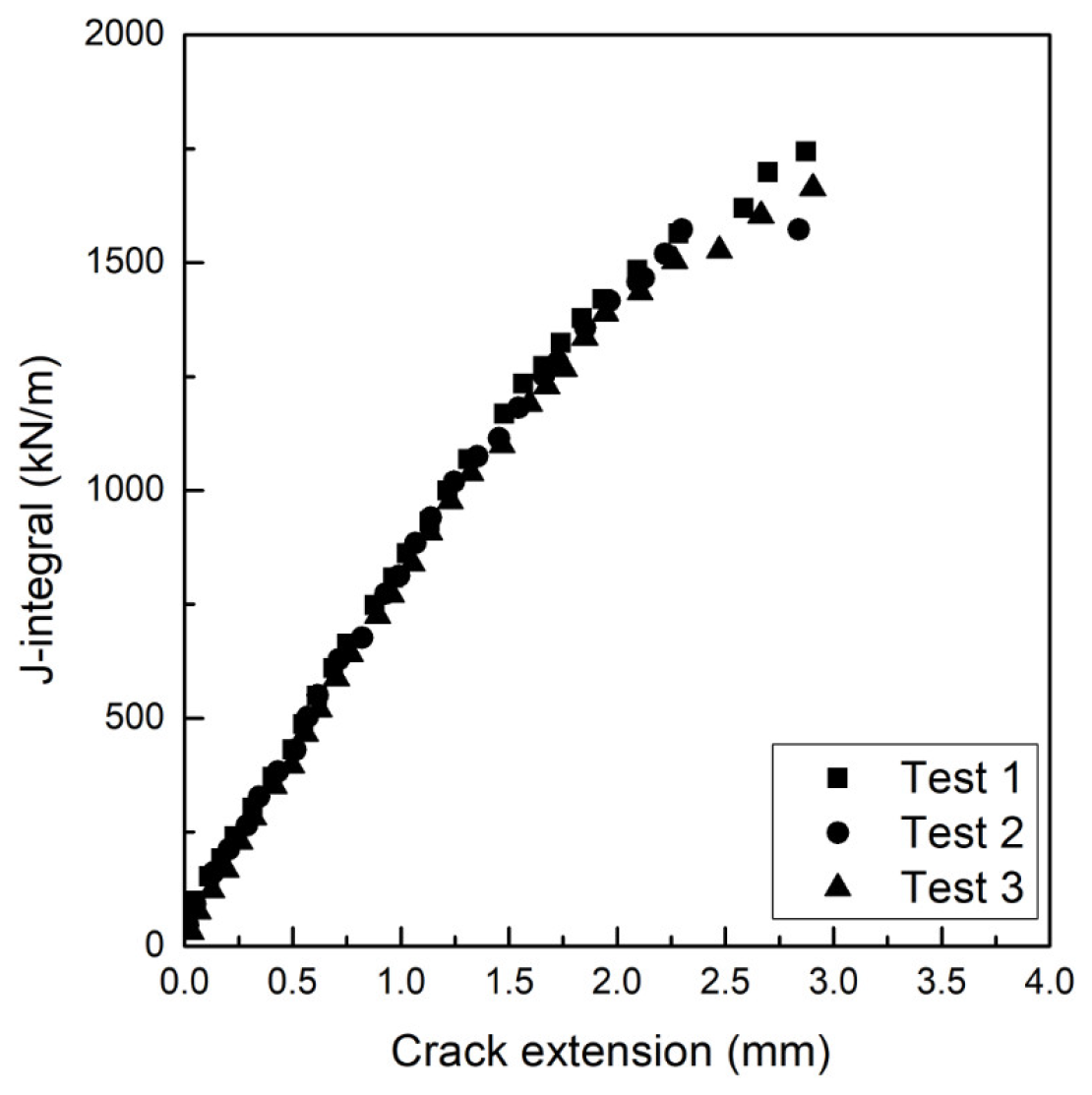
3.2. Calibration of Parameters

The basic material properties for TP304L stainless steel are obtained by tensile tests according to ASTM E 8 [31] with the specimen as shown in Figure 5a. From tensile tests, the yield strength and tensile strength are obtained as 269 MPa and 529 MPa, respectively. The material constants in Equation (2) are determined based on the tensile test results of smooth and notched specimens (Figure 5). A quarter of the FE models for these specimens are constructed to simulate the tensile behaviors, as shown in Figure 6. The simulation results agree well with the test results for four kinds of specimens (Figure 7a). The stress triaxiality and strain in the middle of the specimen are extracted from the FE simulation, as shown in Figure 7b. The area-averaged stress triaxiality is used to fit the relation between critical fracture strain and stress triaxiality for considering the loading history effect, as shown in Figure 7c, and the values of A and B are determined as 4.5 and 0.22, respectively.
A half-model of a 0.5T-CT specimen is constructed to study the effect of the element-size-dependent critical damage parameter ( ω c ), as illustrated in Figure 8a. To accurately capture crack-tip propagation behavior, a fine mesh of C3D8R hexahedral elements was implemented along the crack propagation path. From the simulation, the load–displacement curve and load–crack extension relationship curve of the model can be obtained. Then, based on the J-integral calculation formula provided in ASTM E1820 [4], these simulation data were converted into J-R resistance curves characterizing the material’s fracture toughness.
Figure 8b demonstrates the significant influence of different ωc parameter values on the predicted J-R curves of the CT specimen when a characteristic element size of 0.4 mm is adopted. As shown in Figure 8c, the values of ωc are determined as 0.22, 0.41, and 0.69 for the element size Le = 0.8, 0.4, and 0.2 mm, respectively. These calibrated parameter values were subsequently applied in numerical simulations of ductile crack propagation behavior in full-scale pipelines, providing a critical basis for balancing computational accuracy and efficiency in large-scale pipe models.

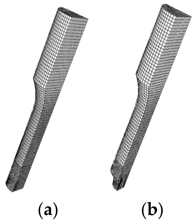
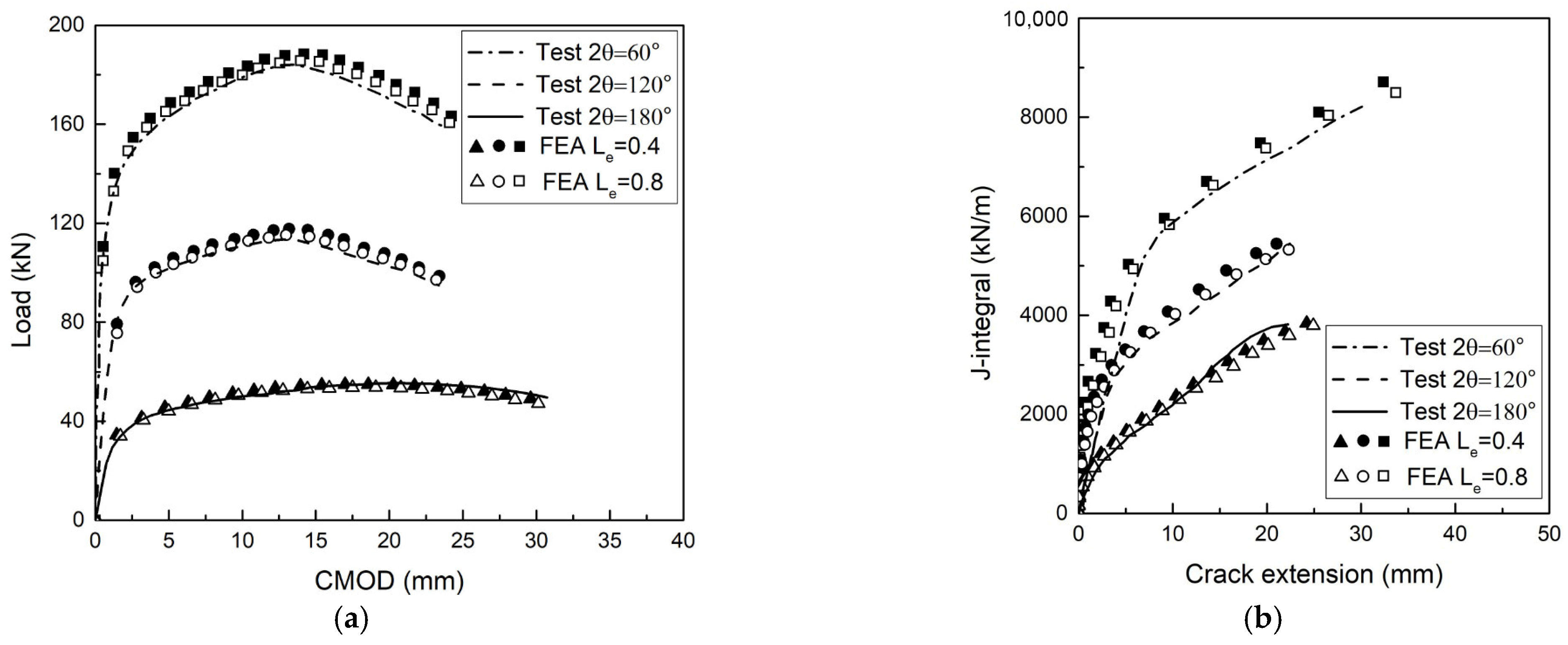
3.3. Simulation Results

The crack growth behavior of a full-scale pipe with a circumferential through-wall crack under a four-point-bending load is simulated based on the parameters calibrated in Section 3.2. A quarter of the FE model for full-scale pipe is constructed because of the symmetry, as shown in Figure 9. The element sizes of Le = 0.2 mm (ωc = 0.69), 0.4 mm (ωc = 0.41), and 0.8 mm (ωc = 0.22) are applied to the cracked surface of full-scale pipes for simulation [32], but a simulation with Le = 0.2 mm fails due to numerical problems. Figure 10 presents the numerical simulation results of the crack propagation diagram for a crack with 2θ = 60°. It can be seen that significant plastic deformation characteristics are exhibited by the crack-tip region, and the crack propagation demonstrates obvious non-uniformity—with the propagation rate in the central region being significantly higher than that at the sides. The underlying mechanism of this phenomenon is primarily related to the stress state distribution along the crack front: in the central region of the crack tip, due to the strong constraint of plane strain, a higher stress triaxiality characteristic is exhibited by this area. Based on the SMCS, it can be inferred that the critical fracture strain value in this region is relatively small. In contrast, near the free surfaces on both sides, the plane stress effect dominates, resulting in relatively lower stress triaxiality. According to the SMCS theory, the critical fracture strain value in these regions is comparatively larger, thereby leading to a slower crack propagation rate.
A comparison between the numerical simulation results and the experimental crack morphology from previous tests shows good agreement, confirming the accuracy and reliability of the SCMC model (Figure 11). The load–CMOD curves obtained from the simulation are compared to those from the full-scale pipe tests, as shown in Figure 12a. The crack length at each time step is measured, and the J-R curves are calculated, as shown in Figure 12b. It can be seen the simulation results agree quite well with the test results, and the element sizes (Le = 0.4 mm and 0.8 mm) show little effect on the simulation results.

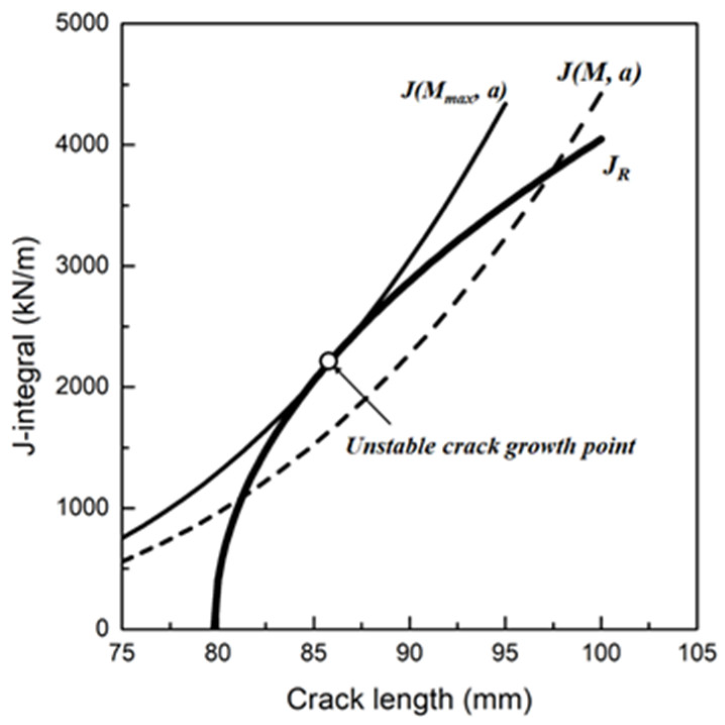
4. LBB Analysis and Discussion

Based on the LBB design philosophy, it is essential to ensure that pipe leaks can be detected by the monitoring system before the pipe completely breaks down. This requires the pipe material to possess sufficient toughness. Austenitic stainless steels such as TP304L exhibit excellent toughness, allowing them to maintain crack resistance even after crack initiation, thereby demonstrating stable crack propagation behavior. This characteristic provides a critical time window for leak detection and pipe repair, effectively preventing catastrophic failures. Under increasing load, the crack undergoes stable propagation until reaching a critical state. When the J-integral at the crack tip reaches the material’s fracture toughness, the crack transitions into unstable propagation. This critical point marks the onset of unstable crack growth, beyond which rapid structural failure occurs. Therefore, accurately predicting the critical load level for unstable crack propagation is of significant engineering importance.
The elastic–plastic fracture mechanics approach based on crack driving force is commonly employed to locate the unstable crack growth point [33,34]. This method analyzes the mechanical behavior of cracked structures under external loading, where the applied J-integral characterizes the crack driving force, while the material’s resistance to crack growth is described by the J-R curve ( J R = J R a ). During stable crack growth, the rate of increase in the crack driving force remains lower than that of the material’s resistance. However, once the driving force’s growth rate exceeds that of the resistance, unstable crack propagation occurs. This critical condition can be expressed as
J ( M , a ) a = J R ( M , a ) a
and can be graphically represented using a crack driving force diagram (CDFD). Figure 13 shows the CDFD for a pipe with an initial crack length of 80 mm. The driving force J ( M , a ) is a function of applied load M and crack length a, and JR is the J-R curve of the cracked structure obtained from the fracture resistance test. Unstable crack growth occurs when the driving force J ( M , a ) is tangent to the J-R curve.
In this study, the driving force J ( M , a ) for a cracked nuclear pipe is obtained according to the GE/EPRI equation [35,36]. Figure 14 shows the CDFD analysis based on the J-R curves from the fracture resistance test of a 0.5T-CT specimen, fracture resistance test of full-scale pipe (2θ = 120°), and numerical simulation of full-scale pipe (2θ = 120°). Jinst represents the point where the crack driving force curve ( J ( M , a ) ) intersects with the J-R curve. The determined values of Jinst and Mmax are shown in Figure 15 It can be seen for the pipe with a large initial crack length (2θ = 180°), the critical load levels predicted based on the J-R curve of the CT specimen are similar to those predicted based on the J-R curve of full-scale pipe, while for the pipe with a short initial crack length (2θ = 60°), the use of the CT specimen to predict critical load levels will cause lots of conservatism. Figure 15 shows that the critical load levels predicted based on the numerical simulations agree quite well with those predicted based on the fracture resistance tests, which demonstrates the validity of numerical ductile fracture simulation in the LBB evaluation of nuclear pipes.

5. Conclusions

In this study, the LBB evaluation of nuclear pipes (SA312 TP304L stainless steel) is performed based on the results of fracture resistance tests and numerical ductile fracture simulations. The conclusions are as follows:
  • The extended SMCS model is employed to accurately simulate the crack propagation behavior in full-scale nuclear pipes with circumferential cracks. By introducing a mesh-dependent critical damage parameter (ωc), the dependence of crack-tip stress–strain fields on mesh size was effectively reduced, enabling the use of larger element sizes in simulations. The ωc values for specific mesh sizes were calibrated by comparing the simulation results with experimental data from CT specimens.
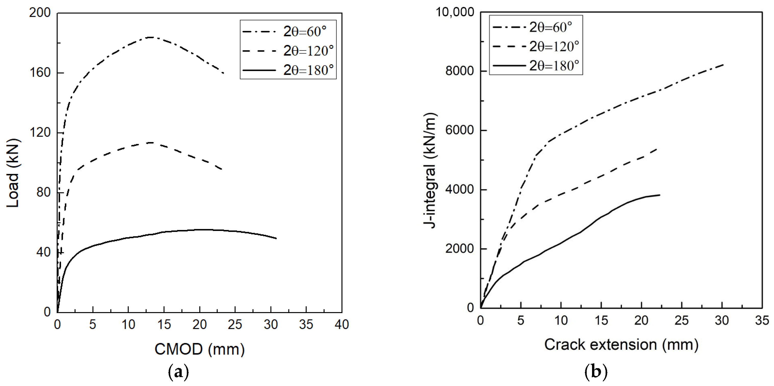
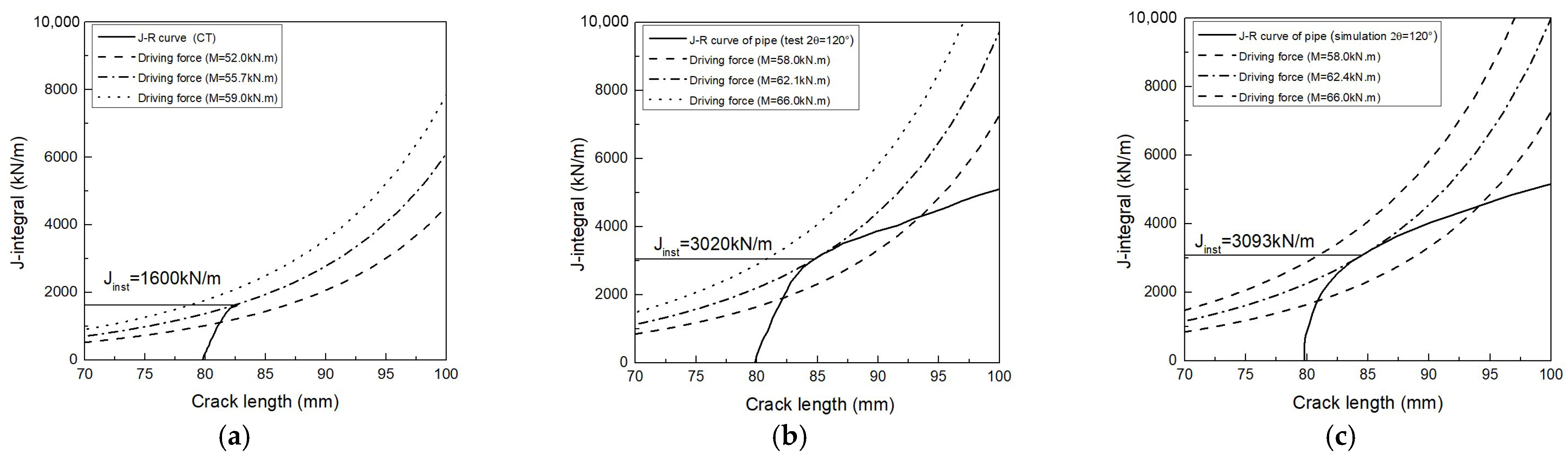
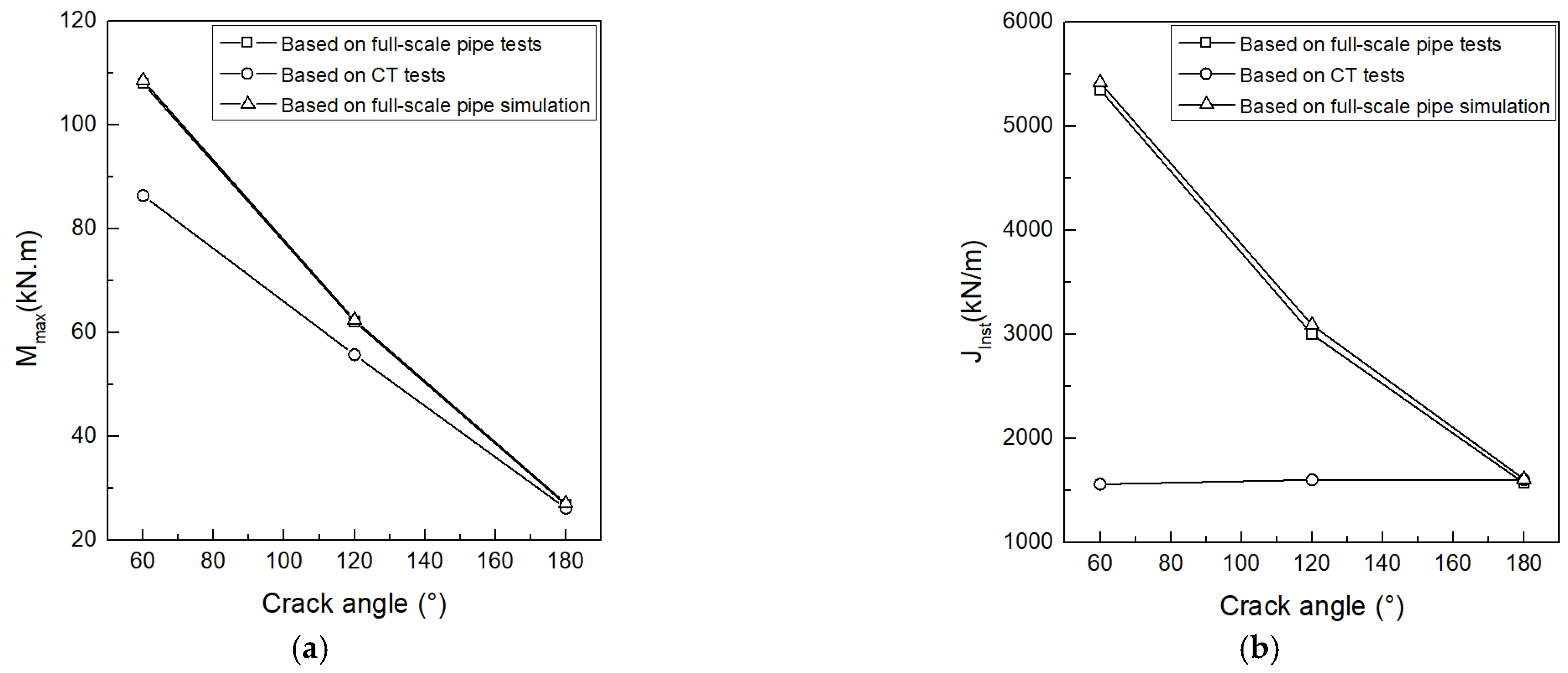
  • Through CDFD analysis, the critical load levels were calibrated for pipes with different initial crack lengths and compared. For a pipe with a large initial crack length (2θ = 180°), the critical load levels in the LBB concept predicted based on the J-R curve of a CT specimen are close to those predicted based on the J-R curve of a full-scale pipe, while for a pipe with a short initial crack length (2θ = 60°), using a CT specimen to predict the critical load level of the pipe may result in significant conservatism.
  • Crack growth behaviors of full-scale nuclear pipes with circumferential cracks are simulated accurately by the extended SMCS model, and the maximum supported load levels predicted based on the simulation results are in good agreement with those predicted based on the full-scale pipe test results. This approach for the design of nuclear pipes by simulating full-scale pipe fractures with an extended SCMS model not only reduces conservatism but also saves significant time and costs.
However, it should be noted that the mesh-dependent critical damage parameter (ωc) is an empirical parameter lacking strong theoretical justification. Moreover, currently, this approach has only been tested on SA312 and TP304L pipes, so its general applicability requires further verification.

Author Contributions

Conceptualization, Y.F. and T.S.; methodology, Y.F. and T.S.; software, B.L.; validation, Y.F. and T.S.; formal analysis, Y.F.; investigation, Y.F.; resources, T.S.; data curation, B.L.; writing—original draft preparation, Y.F.; writing—review and editing, T.S.; visualization, B.L.; supervision, T.S.; project administration, C.-S.S.; funding acquisition, C.-S.S. All authors have read and agreed to the published version of the manuscript.

Funding

This research was funded by the National Research Foundation of Korea (NRF) grant funded by the Korean government (MSIT) (No. 2018R1A2A1A05077886) and the China Postdoctoral Science Foundation (No. 2024M753829).

Data Availability Statement

Data will be made available on request.

Acknowledgments

We acknowledge the financial support provided by the National Research Foundation of Korea (NRF) grant funded by the Korean government (MSIT) (No. 2018R1A2A1A05077886) and the China Postdoctoral Science Foundation (No. 2024M753829).

Conflicts of Interest

The authors declare no conflicts of interest.

References

  1. He, F.; Xiong, F.; Bai, X.; Yang, K.; Lu, X.; Li, B.; Wang, X. Study and analysis of the effect of dynamic load on the application of LBB technology to the primary pipe of reactor coolant system. Nucl. Eng. Des. 2024, 429, 113646. [Google Scholar] [CrossRef]
  2. Blasset, S.; Hartmann, M.; Courtin, E.; Nicaise, N.; Nana, A. Leak-before-break and other concepts of break-exclusion. Int. J. Press. Vessel. Pip. 2024, 209, 105197. [Google Scholar] [CrossRef]
  3. Huh, N.S. New Engineering Method of Non-linear Fracture mechanics Analysis of Circumferential Through-wall Cracked Pipes; Sungkyunkwan University: Seoul, Republic of Korea, 2000. [Google Scholar]
  4. E1820-01; A.S. Standard Test Method for Measurement of Fracture Toughness. ASTM International: West Conshohocken, PA, USA, 2001.
  5. Seok, C.-S.; Kim, S.-Y. A study on the characteristics of fracture resistance curve of ferritic steels. KSME Int. J. 1999, 13, 827–835. [Google Scholar] [CrossRef]
  6. O’Dowd, N.P.; Shih, C.F. Family of crack-tip fields characterized by a triaxiality parameter—I. Structure of fields. J. Mech. Phys. Solids 1991, 39, 989–1015. [Google Scholar] [CrossRef]
  7. O’Dowd, N.P.; Shih, C.F. Family of crack-tip fields characterized by a triaxiality parameter—II. Fracture applications. J. Mech. Phys. Solids 1992, 40, 939–963. [Google Scholar] [CrossRef]
  8. Yang, S.; Chao, Y.J.; Sutton, M.A. Higher order asymptotic crack tip fields in a power-law hardening material. Eng. Fract. Mech. 1993, 45, 1–20. [Google Scholar] [CrossRef]
  9. Chao, Y.J.; Zhu, X.K. J-A2 Characterization of Crack-Tip Fields: Extent of J-A2 Dominance and Size Requirements. Int. J. Fract. 1998, 89, 285–307. [Google Scholar] [CrossRef]
  10. Zhu, X.-K.; Leis, B.N. Bending modified J–Q theory and crack-tip constraint quantification. Int. J. Fract. 2006, 141, 115–134. [Google Scholar] [CrossRef]
  11. Huh, N.S.; Kim, Y.J.; Choi, J.B.; Kim, Y.J.; Kim, Y.J. Prediction of failure behavior for nuclear piping using curved wide-plate test. J. Press. Vessel Technol. Trans. ASME 2004, 126, 419–425. [Google Scholar] [CrossRef]
  12. Shen, T.; Park, K.-t.; Choi, J.-g.; Moon, B.-W.; Koo, J.-M.; Seok, C.-S. Evaluation for fracture resistance curves of nuclear real pipes using curved equivalent stress gradient (curved ESG) specimens. Eng. Fract. Mech. 2017, 169, 89–98. [Google Scholar] [CrossRef]
  13. Liao, F.; Wang, W.; Chen, Y. Ductile fracture prediction for welded steel connections under monotonic loading based on micromechanical fracture criteria. Eng. Struct. 2015, 94, 16–28. [Google Scholar] [CrossRef]
  14. Mundó, I.; Caner, F.C.; Mateo, A. Micromechanical modelling of the elastoplasticity and damage in ductile metals. Int. J. Solids Struct. 2025, 317, 113437. [Google Scholar] [CrossRef]
  15. Kim, M.-S.; Cho, Y.-H.; Jang, H. Numerical modeling of stress-state dependent damage evolution and ductile fracture of austenitic stainless steel. Int. J. Solids Struct. 2025, 318, 113439. [Google Scholar] [CrossRef]
  16. Moattari, M.; Sattari-Far, I.; Persechino, I.; Bonora, N. Prediction of fracture toughness in ductile-to-brittle transition region using combined CDM and Beremin models. Mater. Sci. Eng. A 2016, 657, 161–172. [Google Scholar] [CrossRef]
  17. Zhang, T.; Zhao, Y. A study on the parameter identification and failure prediction of ductile metals using Gurson–Tvergaard–Needleman (GTN) model. Mater. Today Commun. 2023, 34, 105223. [Google Scholar] [CrossRef]
  18. Ding, X.; Wei, X.; Zhang, X.; Hou, Y.; Zhao, F. Ductile fracture prediction of titanium foil based on shear-modified GTN damage model considering size effect. Eng. Fract. Mech. 2025, 323, 111200. [Google Scholar] [CrossRef]
  19. Min, F.; Gao, K.; Huang, H.; Wen, S.; Wu, X.; Nie, Z.; Zhou, D.; Gao, X. Application of the modified GTN model in predicting Taylor impact fracture of 7XXX aluminum alloy. Comput. Struct. 2024, 301, 107457. [Google Scholar] [CrossRef]
  20. Oh, C.-S.; Kim, N.-H.; Kim, Y.-J.; Baek, J.-H.; Kim, Y.-P.; Kim, W.-S. A finite element ductile failure simulation method using stress-modified fracture strain model. Eng. Fract. Mech. 2011, 78, 124–137. [Google Scholar] [CrossRef]
  21. Jeon, J.Y.; Kim, Y.J.; Kim, J.W.; Lee, S.Y. Effect of thermal ageing of CF8M on multi-axial ductility and application to fracture toughness prediction. Fatigue Fract. Eng. Mater. Struct. 2015, 38, 1466–1477. [Google Scholar] [CrossRef]
  22. Youn, G.-G.; Nam, H.-S.; Kim, Y.-J.; Kim, J.-W. Numerical prediction of thermal aging and cyclic loading effects on fracture toughness of cast stainless steel CF8A: Experimental and numerical study. Int. J. Mech. Sci. 2019, 163, 105120. [Google Scholar] [CrossRef]
  23. Chi, W.-M.; Kanvinde, A.M.; Deierlein, G.G. Prediction of Ductile Fracture in Steel Connections Using SMCS Criterion. J. Struct. Eng. 2006, 132, 171–181. [Google Scholar] [CrossRef]
  24. Oh, C.-K.; Kim, Y.-J.; Baek, J.-H.; Kim, W.-s. Development of stress-modified fracture strain for ductile failure of API X65 steel. Int. J. Fract. 2007, 143, 119–133. [Google Scholar] [CrossRef]
  25. Kiran, R.; Khandelwal, K. Gurson model parameters for ductile fracture simulation in ASTM A992 steels. Fatigue Fract. Eng. Mater. Struct. 2014, 37, 171–183. [Google Scholar] [CrossRef]
  26. Kanvinde, A.M.; Deierlein, G.G. The Void Growth Model and the Stress Modified Critical Strain Model to Predict Ductile Fracture in Structural Steels. J. Struct. Eng. 2006, 132, 1907–1918. [Google Scholar] [CrossRef]
  27. Kanvinde, A.M. Micromechanical Simulation of Earthquake Induced Fractures in Steel Structures; Stanford University: Stanford, CA, USA, 2005. [Google Scholar]
  28. Nam, H.-S.; Oh, Y.-R.; Kim, Y.-J.; Kim, J.-S.; Miura, N. Application of engineering ductile tearing simulation method to CRIEPI pipe test. Eng. Fract. Mech. 2016, 153, 128–142. [Google Scholar] [CrossRef]
  29. Seok, C.S. Real-Scale Pipe Testing and Knowledge and Information Database on the Piping of Nuclear Power Plant for the LBB Design; National Research Foundation of Korea: Daejeon, Korea, 2012. [Google Scholar]
  30. Zahoor, A.; Kanninen, M.F. A Plastic Fracture Mechanics Prediction of Fracture Instability in a Circumferentially Cracked Pipe in Bending—Part I: J-Integral Analysis. J. Press. Vessel Technol. 1981, 103, 352–358. [Google Scholar] [CrossRef]
  31. E8-01; A.S. Standard test method for tension testing of metallic materials. ASTM International: West Conshohocken, PA, USA, 2007.
  32. Iqbal, S.; Siddique, M.; Hamza, A.; Murtaza, N.; Pasha, G.A. Computational analysis of fluid dynamics in open channel with the vegetated spur dike. Innov. Infrastruct. Solut. 2024, 9, 345. [Google Scholar] [CrossRef]
  33. Kim, Y.J.; Jung, H.D. Integrity evaluation of pressure vessel and piping system of nuclear power plant. KSME Int. J. 1991, 31, 244–250. [Google Scholar]
  34. Gong, N.; Wang, G.Z.; Xuan, F.Z.; Tu, S.T. Leak-before-break analysis of a dissimilar metal welded joint for connecting pipe-nozzle in nuclear power plants. Nucl. Eng. Des. 2013, 255, 1–8. [Google Scholar] [CrossRef]
  35. Kumar, V.; German, M.D.; Wilkening, W.W.; Andrews, W.R.; Mowbray, D.F. Advances in Elastic-Plastic Fracture Analysis; General Electric Co.: Schenectady, NY, USA, 1984. [Google Scholar]
  36. Kumar, V.; German, M.D.; Shih, C.F. An Engineering Approach for Elastic-Plastic Fracture Analysis; General Electric Company: Schenectady, NY, USA, 1981. [Google Scholar]
Figure 1. Geometry of 0.5T-CT specimen.
Applsci 15 07010 g001
Figure 2. J-R curves of 0.5T-CT specimens [29].
Applsci 15 07010 g002
Figure 3. Loading condition for full-scale pipe tests [29].
Applsci 15 07010 g003
Figure 4. Full-scale pipe test results: (a) load–CMOD curves; (b) J-R curves [29].
Applsci 15 07010 g004
Figure 5. Tensile specimens: (a) smooth bar; (b) notched bar (R = 1.5, 3, 6 mm).
Applsci 15 07010 g005
Figure 6. Tensile specimens: (a) smooth bar; (b) notched bar (R = 6 mm).
Applsci 15 07010 g006
Figure 7. Test and simulation results for smooth and notched bars: (a) engineering stress–strain curves; (b) stress triaxiality–equivalent plastic strain curves; (c) fracture strain–stress triaxiality curve.
Applsci 15 07010 g007
Figure 8. FE simulation for determining element-size-dependent parameter ωc: (a) FE model for CT specimen; (b) effect of ωc on J-R curves of CT specimen when Le = 0.4 mm; (c) value of ωc according to Le.
Applsci 15 07010 g008
Figure 9. Numerical simulation model for full-scale pipe tests.
Applsci 15 07010 g009
Figure 10. Numerical simulation results for the evaluation of a crack in the full-scale pipe with 2 θ = 60°.
Applsci 15 07010 g010
Figure 11. Comparison of full-scale pipe fracture morphology between experiments and numerical simulations [29].
Applsci 15 07010 g011
Figure 12. Comparison of test and simulation results of full-scale pipes: (a) load–CMOD curves; (b) J-R curves.
Applsci 15 07010 g012
Figure 13. Crack driving force diagram (CDFD).
Applsci 15 07010 g013
Figure 14. CDFD analysis: (a) based on the J-R curves from the fracture resistance test of a 0.5T-CT specimen; (b) based on the J-R curves from the fracture resistance test of a full-scale pipe (2θ = 120°); (c) based on the J-R curves from the numerical simulation of a full-scale pipe (2θ = 120°).
Applsci 15 07010 g014
Figure 15. Comparison of CDFD analysis results: (a) comparison of Mmax; (b) comparison of Jinst.
Applsci 15 07010 g015
Disclaimer/Publisher’s Note: The statements, opinions and data contained in all publications are solely those of the individual author(s) and contributor(s) and not of MDPI and/or the editor(s). MDPI and/or the editor(s) disclaim responsibility for any injury to people or property resulting from any ideas, methods, instructions or products referred to in the content.

