Emotion Recognition from Speech in a Subject-Independent Approach

Abstract

The aim of this article is to critically and reliably assess the potential of current emotion recognition technologies for practical applications in human–computer interaction (HCI) systems. The study made use of two databases: one in English (RAVDESS) and another in Polish (EMO-BAJKA), both containing speech recordings expressing various emotions. The effectiveness of recognizing seven and eight different emotions was analyzed. A range of acoustic features, including energy features, mel-cepstral features, zero-crossing rate, fundamental frequency, and spectral features, were utilized to analyze the emotions in speech. Machine learning techniques such as convolutional neural networks (CNNs), long short-term memory (LSTM) networks, and support vector machines with a cubic kernel (cubic SVMs) were employed in the emotion classification task. The research findings indicated that the effective recognition of a broad spectrum of emotions in a subject-independent approach is limited. However, significantly better results were obtained in the classification of paired emotions, suggesting that emotion recognition technologies could be effectively used in specific applications where distinguishing between two particular emotional states is essential. To ensure a reliable and accurate assessment of the emotion recognition system, care was taken to divide the dataset in such a way that the training and testing data contained recordings of completely different individuals. The highest classification accuracies for pairs of emotions were achieved for Angry–Fearful (0.8), Angry–Happy (0.86), Angry–Neutral (1.0), Angry–Sad (1.0), Angry–Surprise (0.89), Disgust–Neutral (0.91), and Disgust–Sad (0.96) in the RAVDESS. In the EMO-BAJKA database, the highest classification accuracies for pairs of emotions were for Joy–Neutral (0.91), Surprise–Neutral (0.80), Surprise–Fear (0.91), and Neutral–Fear (0.91).

1. Introduction

In today’s rapidly evolving technological landscape, the ability to recognize emotions from the human voice is increasingly crucial, especially in the realm of human–machine communication [1,2]. Equipping computers with the ability to comprehend human emotions aids in better tailoring responses to our needs and personalizing our technological experiences. This capability holds significant importance across various fields. For instance, it supports individuals facing communication challenges, such as those with autism, in more effectively expressing and understanding emotions [3,4]. In healthcare, monitoring patients’ emotions can facilitate the early detection of issues like depression [5]. Robots equipped with emotion recognition can more effectively collaborate with us, providing assistance in domestic settings, education, or healthcare by adapting their behavior to our mood and requirements [6]. Integrating voice emotion recognition with other technologies, such as gesture recognition, enables the development of even more sophisticated interfaces [7,8,9,10].

The human voice is an incredibly rich source of information about our emotions, making it an attractive medium for emotion recognition. This attractiveness stems from the fact that the way we speak—our tone, pace, volume, and modulations—unconsciously changes depending on our emotional state [11,12], allowing voice analysis to offer insights into a person’s feelings, often with greater precision than the observation of behavior or facial expressions. However, despite its potential, recognizing emotions from the voice through machines presents challenges. The first challenge is the complexity of the human voice itself, which can vary significantly due to factors such as age, gender, health status, or even accent [12,13], complicating the creation of a universal model capable of effectively interpreting emotions. Moreover, emotions are not always expressed clearly. Different cultures may manifest emotions in various ways, and individual differences in emotional expression can mean that what signifies joy for one person might be considered neutral for another [14]. Thus, machines must learn to recognize the subtle nuances in voice, requiring advanced machine learning algorithms and extensive datasets for training. Additionally, emotions can be concealed or masked by the speaker, further complicating the task. People often regulate their tone of voice to hide their true feelings. Finally, the implementation of a voice emotion recognition system in practical applications not only demands advanced technology but also the consideration of privacy and ethics. Matters such as consent for voice analysis and the protection of personal data are key to the societal acceptance of such technologies.

Despite these challenges, the development of voice emotion recognition technology opens up new possibilities in various fields, from enhancing human–machine interactions and supporting mental health diagnosis and therapy to applications in the entertainment and marketing sectors. Therefore, addressing these challenges represents an important research direction in the field of artificial intelligence.

2. Related Articles

As of 14 May 2025, a search of the Scopus database using the keywords emotion, speech, and recognition resulted in the identification of 19,550 documents, including scientific articles and conference materials published since 2015. This clearly indicates a growing interest among researchers in the detection of emotions from human speech. The total number of only scientific articles related to this topic reached 7272, highlighting the intense scientific effort to understand and interpret the emotional aspects of speech. User interface development and support for medical diagnosis and therapy are just some of the areas that could benefit from advances in speech emotion recognition [15,16]. The availability of databases may encourage researchers to experiment with new algorithms for processing, classifying, and analyzing speech signals, with the hope of achieving even better results.

During their research, the authors utilize various databases, which significantly differ in terms of registration method, the number of represented emotions, the number of individuals whose speech has been recorded, language, and accents [1,17]. The most frequently used databases in emotion recognition studies are IEMOCAP, SAVEE, the RAVDESS, Emo-DB, and CASIA. IEMOCAP contains audio-visual recordings of ten actors (five males and five females) speaking in English, exhibiting anger, happiness, excitement, sadness, frustration, fear, surprise, and neutrality [18]. SAVEE focuses on audio-visual recordings of four English-speaking males expressing anger, disgust, sadness, fear, happiness, surprise, and neutral [19]. The RAVDESS includes recordings from twelve male and twelve female speakers expressing eight emotions in English: happiness, sadness, anger, fear, surprise, disgust, calmness, and neutrality. [20]. Emo-DB centers on recordings of five males and five females speaking in German, expressing anger, boredom, disgust, fear, happiness, sadness, and neutrality [21]. CASIA features recordings of two males and two females speaking in Chinese, expressing anger, fear, happiness, neutrality, sadness, and surprise [22].

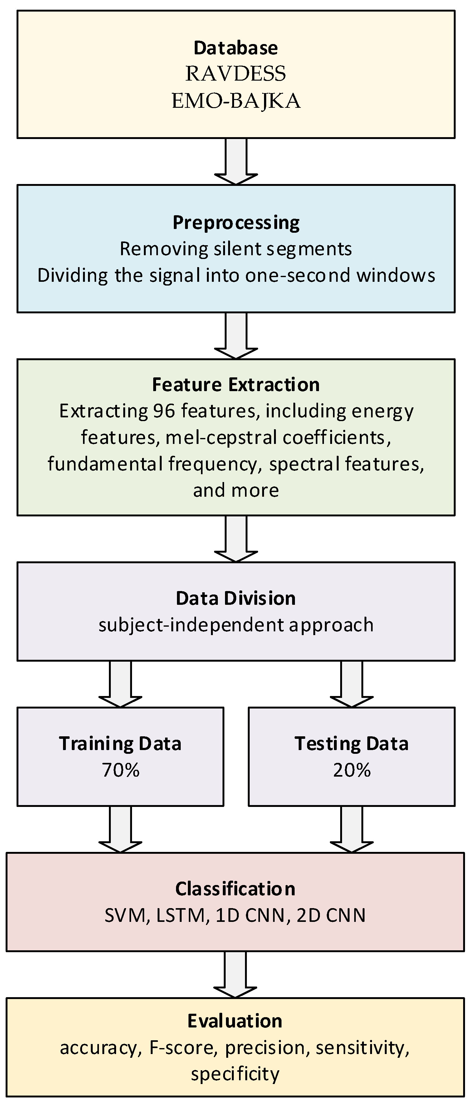
Emotion recognition from voice is a process that can be divided into three main stages: preprocessing, feature extraction, and classification [23,24]. Each of these stages is crucial for the effective identification of emotions. Preprocessing aims to prepare audio data for further analysis. This stage involves reducing noise and interference, which is essential for improving the quality of the recording [25]. Moreover, amplitude normalization helps unify the volume levels of all samples, making the feature extraction process more consistent. Another common step is windowing, which involves dividing long recordings into shorter segments, usually containing single statements or phrases [26]. Raw audio signals can be used directly, as in [27], where a deep learning architecture termed RNN–CNN was designed to perform speech emotion recognition. Typically, the feature extraction stage is performed. This process involves extracting significant attributes from the audio signal that can be used to identify emotions [28,29,30]. The most important features include prosodic features such as pitch, intensity, and speech rate [31,32]. These features often change depending on the emotion; for example, happiness can be expressed through a faster speech rate and higher pitch. Spectral features, such as formants and mel-frequency cepstral coefficients (MFCCs), are also commonly used to analyze the properties of speech and music [33,34]. The final stage is classification, where the extracted features are assigned to a specific category of emotion [7,35]. Among the most popular classification methods are support vector machines (SVMs), which are effective in distinguishing between different emotions, even with a relatively small number of features [36,37,38], and artificial neural networks (ANNs), especially those utilizing deep learning. Neural networks such as convolutional neural networks (CNNs), long short-term memory (LSTM), and gated recurrent units (GRUs) are capable of automatically extracting features from raw audio data and achieving high accuracy in emotion recognition [39,40]. In [41], the researchers examined whether a compact deep neural network ensemble (combining a CNN and CNN_Bi-LSTM) that leverages traditional hand-crafted features such as the ZCR, RMSE, Chroma STFT, and MFCC could surpass the performance of models that rely on automated feature extraction, such as spectrogram-based approaches. The effectiveness of their method was tested across five standard datasets: the RAVDESS, TESS, SAVEE, CREMA-D, and EmoDB. Their findings showed that the proposed ensemble model generally achieved superior results compared to both individual and spectrogram-based models on these datasets. Additionally, there is an effort to utilize pretrained networks and apply transfer learning techniques [42,43]. The effectiveness of voice emotion recognition depends on each of these stages and on the algorithms’ ability to generalize across different conditions and environments. Different authors’ studies have employed varying numbers of recognized emotions, as well as diverse preprocessing methods, segmentation techniques, feature extraction and classification approaches, and testing strategies. For this reason, despite the abundant scientific literature, it is challenging to find reliable comparisons of classification results that could indicate greater or lesser effectiveness of various voice-based emotion classification methods. The literature includes several comprehensive reviews on voice emotion recognition [1,17,44,45,46,47,48].

3. Aim of the Article

Speech recognition using AI in a subject-independent approach remains a significant challenge. Despite many years of technological development, most existing solutions achieve high accuracy only when tailored to specific users (subject-dependent). This article aims to critically and comprehensively analyze the current capabilities of algorithms to recognize emotions from a speaker’s voice in a subject-independent approach. Various approaches used in the voice analysis process were examined, including the latest machine learning and artificial intelligence algorithms applied to identify subtle nuances in tone, pace, volume, and other characteristic voice features. The research utilized two databases, one in Polish and the other in English, recorded in different ways. Our studies focus on selected short speech signals. Special attention was given to how to divide the data so that the results are comparable to a real case of emotion recognition. This means that the test data do not include examples from individuals who participated in the training process (subject-independent). Such an approach aims to ensure that the model can be generalized to new, unknown speech signals. Dividing the data into training and test sets in this way allows for a more accurate assessment of the model’s ability to recognize speech in conditions closer to reality. The general research framework presented in the article is shown in Figure 1.

We expect to achieve worse results than those presented in many articles, but we hope that the obtained results will allow a reliable assessment of the ability to recognize emotions from short speech fragments. The goal of our research is primarily to understand the limitations of existing methods and identify opportunities for further development in the field of automatic emotion recognition. The results, even if not comparable with the best available models, will provide valuable insights into how emotions manifest in short speech segments and how they can be effectively recognized.

4. Materials

In our research, we decided to focus on two databases: one recorded in English and the other in Polish. This choice was motivated by the desire to explore how emotion recognition technologies perform in analyzing voice across different languages, allowing for a better understanding of the universality and limitations of the methods used. The English language database provides access to a wide range of voice examples from 24 speakers. In contrast, the Polish language database offers data from 26 speakers, enabling the examination of emotion recognition specifics for a language and culture significantly less represented in global research. One of the key differences between the studied databases is the manner of speech presentation. In the English-language database, actors always spoke the same sentences, simulating emotions. In the Polish database, actors expressed emotions through various spoken sentences. Recordings in the Polish database are characterized by a significantly greater diversity. However, it is important to remember that each database was developed based on simulated emotions, which often differ from real emotions expressed without emphasizing them.

4.1. RAVDESS—English-Language Database

The Ryerson Audio-Visual Database of Emotional Speech and Song (RAVDESS) is a valuable resource for research on emotional expression in speech and song [20]. It contains 1440 audio files, each recorded by one of 24 professional actors (12 women and 12 men), expressing emotions through two sentences in a neutral North American accent. For the experiments, only files related to spoken emotions were selected. Each actor uttered one of two phrases (“Kids are talking by the door”; “Dogs are sitting by the door”). Each of the seven expressed emotions—calm, joy, sadness, anger, fear, surprise, and disgust—is represented by 96 recordings. The database also includes recordings with a neutral tone. The recordings are saved in .wav format with a sampling rate of 48 kHz and 16-bit resolution.

4.2. EMO-BAJKA—Polish-Language Database

The EMO-BAJKA database was created for the purpose of emotion recognition in the Polish language [49]. It contains 260 audio files. The emotions and the number of recordings in the database are as follows: neutral (35 recordings), joy (26 recordings), sadness (55 recordings), fear (19 recordings), surprise (54 recordings), anger (61 recordings), and boredom (10 recordings). The recordings were made by 26 individuals. Two sources were used to create the database. The first and primary source was fairy tales from the archives of Polish Catholic Radio. The recordings were made by teenagers from high schools and lyceums. The second source consists of radio dramas available on the Internet, performed by professional adult actors. The recordings feature both male (121) and female (139) voices. The speech signal recordings range from one to six seconds in length. They are saved in .wav format with a sampling rate of 44 kHz and 16-bit resolution.

4.3. Human Ability to Recognize Emotions

To assess how well the recorded emotions allow for their differentiation, experiments on emotion recognition by humans were first conducted. These involved participants listening to recordings and assigning specific emotions to them. The study involved 10 Polish-speaking individuals, raised in Central European culture, aged 18–50 years. Each person evaluated 80 randomly selected recordings. Two approaches to emotion recognition were tested: based on entire recordings and recordings divided into one-second segments. The results of emotion recognition for different databases are presented in

Table 1. Results of emotion recognition in voice recordings by humans.

Database	1 s	The Entire Statement
EMO-BAJKA	0.40 +/− 0.18	0.58 +/− 0.14
RAVDESS	0.28 +/− 0.14	0.61 +/− 0.22

. It should be stated that the primary objective of this experiment was not to conduct an extensive psychological study on a broad population but rather to gain general insight into how people manage emotion recognition based on very brief (one-second) voice segments compared to complete utterances. This test also aimed to provide an interpretive context for the results produced by the learning models—demonstrating that humans, too, exhibit low accuracy in emotion recognition from very brief voice snippets.

The obtained results for the two databases, EMO-BAJKA and the RAVDESS, indicate differences in the effectiveness of emotion recognition depending on the length of the analyzed recording segment. For the EMO-BAJKA database, the accuracy of emotion recognition based on one-second segments is 0.40 (with a standard deviation of 0.18), whereas for entire statements, the accuracy is higher, at 0.58 (with a standard deviation of 0.14). A similar pattern is observed in the case of the RAVDESS, where the accuracy for one-second segments is 0.28 (with a standard deviation of 0.14), and for entire statements, it is 0.61 (with a standard deviation of 0.22). These results suggest that the participants were able to more accurately recognize emotions when analyzing entire statements, compared to short, one-second segments.

In the case of the database containing Polish-language recordings, we observe an interesting phenomenon that significantly influenced the emotion recognition process. In the recorded Polish statements, keywords or phrases directly indicating emotions, such as “I’m scared” (“boję się”), “I’m happy” (“cieszę się”), or the expressive “hooray” (“hura”), often appeared, which could directly suggest to listeners the type of emotion presented by the speaker. Such unambiguous semantic cues, acting as clear emotional signals, undoubtedly made it easier for participants to identify emotions. It is noteworthy that such direct expressions suggesting emotions did not occur in the English-language database. The absence of such clear emotional indicators in English-language statements required the experiment participants to focus more on other aspects of the message, such as voice tone, speech pace, or intonation, to accurately determine the speaker’s emotions.

The results show that human emotion recognition from brief one-second voice clips is quite poor. Although using full utterances boosts performance, multiclass emotion classification remains challenging even for humans. This underscores the complexity of the task and supports further investigation into automated methods.

5. Methods

This chapter describes the preprocessing algorithms for speech recordings, feature extraction methods from audio signals, and classification methods applied by the authors in their research.

5.1. Preprocessing of Signals

During preprocessing, silent segments preceding and following speech were removed, and no further operations were applied. The speech signal was then divided into one-second windows with shifts in either 0.1 or 0.5 s. Selecting a one-second window strikes a balance between capturing local manifestations of emotional expression and providing an acoustically rich, statistically stable sample in a subject-independent setup. Elementary speech features—such as fundamental frequency, energy modulations, articulation rate, and cepstral fluctuations—evolve over a few hundred milliseconds, but their reliable estimation requires observation spanning at least two to three full prosodic cycles [50]. A one-second window typically contains three to four syllables, encompassing a full intonational arc and brief micronarrative pauses [51]. Shorter segments (250–500 ms) in our tests increased feature variance and degraded classification performance, since isolated plosive consonants or recording artifacts exerted a disproportionate influence on the feature vector. Conversely, windows longer than one second proved impractical: although the RAVDESS includes two-second phrases, EMO-BAJKA contains them only sporadically, drastically reducing the number of training samples. Moreover, longer segments blend speech with silence and dynamic shifts, blurring the emotional signal and amplifying lexical dependencies, which in a subject-independent context leads to overfitting to specific speakers [52]. Thus, one-second windows with a 100 ms shift satisfy three key criteria: they provide sufficient examples for training and validation; they isolate purely acoustic carriers of emotion without semantic context; and they ensure stable estimation of prosodic and spectral parameters while preserving their local character [53].

5.2. Feature Extraction

There are many feature extraction methods that can be used to analyze emotions in speech. The choice of appropriate methods depends on the specifics of the task and the characteristics of the data. Speech signal energy is measured as the sum of the squared amplitude values of samples within a frame [54]. In practice, the logarithm of energy is often used to better reflect human perception of loudness. High signal energy may indicate stronger emotions, such as anger or excitement, while lower energy may be characteristic of calm or sad states. Mel-frequency cepstral coefficients (MFCCs) are calculated by transforming the power spectrum of the speech signal onto the mel scale, which better mirrors the human ear’s perception of sound [55,56,57,58]. This process begins by dividing the speech signal into short frames. For each frame, a Fourier transform is calculated to obtain the power spectrum. Then, this spectrum is filtered using a set of triangular filters evenly spaced on the mel scale. The energy from each filter is logarithmized, and a discrete cosine transform (DCT) is applied to obtain cepstral coefficients. In our research we used the first twelve MFCCs, which are commonly employed to characterize the speech signal. The delta MFCC, the first-order derivative of MFCCs over time, represents the rate of change in spectral features. Delta–delta MFCCs, also known as the “acceleration” of MFCCs, are the second-order derivatives of MFCCs over time. They represent the rate of change in the delta parameters. The zero-crossing rate (ZCR) measures how many times the signal waveform crosses zero within a fixed time window and correlates with the relative energy in higher versus lower frequencies [29,59]. The speech signal spectrum is characterized by certain local maxima and minima. The local maxima are called formants and are denoted by the letter F followed by a number indicating the formant number. The laryngeal tone—also called the fundamental frequency (F0)—is the rate at which the vocal folds vibrate during voiced speech. It corresponds to the lowest-frequency component (the first harmonic) of the glottal excitation signal and is perceived by listeners as the speaker’s pitch [31]. The speaker’s emotional state also affects this parameter. The spectrum’s center of gravity, also known as the weighted mean frequency, is a measure that determines the average frequency of the sound spectrum, weighted by amplitude [60]. Spectral flux measures the degree of change in the power spectrum of the speech signal between consecutive frames [61,62]. Spectral roll-off is the frequency point below which the accumulated spectrum energy reaches a specified percentage (e.g., 80%, 50%, 30%) of the total energy [63,64]. This allows for the identification of dominant frequency bands in the speech signal.

Table 2. Description of the calculated features.

Feature	Description	Number of Features
Energy features	RMS value (RMS), mean value of energy (Eavg), maximum value of energy (Emax), minimum value of energy (Emin), energy variance (Evar), mean value of RMS value (RMSavg), maximum of RMS value (RMSmax), minimum of RMS value (RMSmin), variance of RMS value (RMSvar), mean logarithm of energy value (lEavg), variance of logarithm of energy (lEvar), maximum value of logarithm of energy (lEmax), minimum value of logarithm of energy (lEmin)	13
Mel-cepstral features	Dcavg (Dcavg), variance of delta coefficient (Dcvar), maximum value of delta coefficient (Dcmax), minimum value of delta coefficient (Dcmin), mean value of delta–delta coefficient (Ddcavg), variance of delta–delta coefficient (Ddcvar), maximum value of delta–delta coefficient (Ddcmax), minimum value of delta–delta coefficient (Ddcmin), mean value of the i-th mel-cepstral coefficient (Mc(i)avg), variance value of the i-th mel-cepstral coefficient (Mc(i)var), maximum value of the i-th mel-cepstral coefficient (Mc(i)max), minimum value of the i-th mel-cepstral coefficient (Mc(i)min)	56
Zero crossing density	Mean value of zero crossings density (GP0avg), variance of zero crossings density (GP0var), maximum value of zero crossings density (GP0max), minimum value of zero crossings density (GP0min)	4
Fundamental frequency	Fundamental frequency (F0), mean value of the fundamental frequency (F0avg), variance of the fundamental frequency (F0var), maximum value of the fundamental frequency (F0max), minimum value of the fundamental frequency (F0min)	5
Other spectral features	Mean value of the center of gravity of the spectrum (SCWavg), variance of the center of gravity of spectrum (SCWvar), maximum value of the center of gravity of spectrum (SCWmax), the mean value of spectral flux (SFavg), variance of spectral flux (SFvar), maximum value of spectral flux (SFmax), mean value of spectral roll off for p threshold (SRO(p)avg), variance of spectral roll off for p threshold (SRO(p)var), maximum value of spectral roll off for p threshold (SRO(p)max), minimum value of spectral roll off for p threshold (SRO(p)min)	18

presents a description of the calculated features (where i represents the i-th mel-cepstral coefficient i = 1 to 12, and p for spectral roll-off specifies how much of the frequencies are concentrated below a given energy threshold p = 80%, 50%, or 30%). In total, 96 features were calculated. Each of these features provides information about the speech signal that can be utilized for emotional analysis. By combining a variety of feature extraction methods, speech emotion recognition systems can achieve high accuracy in identifying emotional states. All extracted features for the RAVDESS and EMO-BAJKA dataset, including the training, validation, and test splits, have been made available on the website: https://github.com/kolodzima/EmotionRecognitionSpeech (accessed on 11 June 2025).

5.3. Applied Classification Methods

The support vector machine with a cubic kernel (cubic SVM) is an effective tool for classifying emotions based on the analysis of vocal features, especially when utilizing many different features [65,66]. The choice of this method is based on its adaptive properties and the ability to handle high-dimensional data. The cubic SVM is valued for its ability to efficiently classify data that are not linearly separable in the input space. By transforming data into a higher-dimensional space, the cubic SVM enables finding a hyperplane that best separates the data classes. The cubic kernel further enhances the model’s ability to deal with the complexity and nonlinearity of vocal features, resulting in higher classification accuracy.

Long short-term memory (LSTM) is a highly effective method for classifying vocal features to distinguish emotions, due to its properties of sequential data processing and the ability to capture temporal dependencies in the data [67,68]. The LSTM network used in the studies begins with an input layer. The network then utilizes two bidirectional LSTM layers, each with 150 units. The first of these layers returns a sequence output, maintaining sequential information at every time step, which is vital for processing information with context in both directions of the sequence. The second bidirectional LSTM layer is configured to return only the last output value, useful for summarizing information from the entire sequence into a single vector. In the next stage, the network uses a fully connected layer, with the number of neurons equal to the number of labels in the training set. This layer aims to map the accumulated features to the appropriate classes. Then, a softmax layer transforms the output from the fully connected layer into a probability distribution, a typical approach in classification, allowing the output to be interpreted as the probability of belonging to particular classes [69]. The Adam optimization algorithm is used to update the model’s weights, a commonly recognized choice for its efficiency and convergence speed in various tasks [70]. The data are shuffled before each epoch, helping prevent overfitting by ensuring the model does not learn irrelevant details of a specific order of training data. For training the LSTM network, two groups of audio signal features were used: mel-frequency cepstral coefficients—12 coefficients and pitch (fundamental frequency). Other features that form sequences (energy and spectral features) were also experimented with, but their application did not improve classification results.

Convolutional neural networks can also be successfully applied to the analysis of audio data [71]. They reduce data dimensionality while preserving key information essential for emotion classification. CNNs are also less sensitive to shifts and deformations in the input data, which is vital in sound analysis where emotions can be expressed differently by various speakers. This resistance to variability in data makes CNNs more versatile and adaptive compared to other classification methods. Finally, the ability of CNNs to learn a hierarchy of features—from simple to increasingly complex—makes them exceptionally good at capturing the emotional complexity contained in the human voice. This allows for a deep understanding and interpretation of subtle acoustic signals that differentiate emotions.

In our research, we utilized CNNs for processing calculated features arranged in a vector (1D CNN) and, in the next step, for processing images—spectrograms (2D CNN). The first case, the 1D CNN, begins with an input layer sized 96 × 1. Then, data flows through two 1D convolutional layers with filters sized 96 × 1 and 16 × 1 for the first layer and 16 × 1 and 32 × 1 for the second, where both are set with ‘padding’ to ‘same’. This means that zeros are added around the input feature maps so that the output has the same height and width as the input. This helps preserve spatial information and simplifies the design of deeper networks. Each convolutional layer is connected to a batch normalization layer, which helps stabilize the learning process by normalizing the output from the preceding layer, and a ReLU activation layer. At the end of the architecture is a fully connected layer with 8 neurons, aimed at aggregating features into a form that enables classification, followed by a softmax layer, transforming the results into a probability distribution of belonging to specific classes. The training of the model is conducted using the Adam optimizer. An initial learning rate set at 0.001 and a maximum number of epochs at 50 allow for gradual adjustment of the model weights in the learning process.

A convolutional neural network (2D CNN) is then used for processing images—spectrograms. The first layer of the 2D CNN network accepts images in the form of spectrograms. The spectrograms are preprocessed into grayscale. Subsequently, three sets of layers consisting of a 2D convolutional layer, a ReLU layer, and a normalization layer are applied. The first convolutional layer has 3 × 3 filters, with ‘padding’ set to ‘same’, meaning that the convolution output will have the same size as its input. After each set of convolutional layers, a 2D maxPooling layer is applied, which reduces spatial dimensions by selecting the maximum value from a 2 × 2-pixel square. This is followed by two more convolutional layers with a larger number of filters (16 and 32, respectively), also with ReLU activation and normalization, and after the second of these, a dropout layer is additionally applied with a dropout probability of 20%. Dropout prevents overfitting by randomly disabling neurons during training. The network ends with a fully connected layer, which has a number of neurons equal to the number of classes, followed by a softmax layer, transforming the results into a probability distribution. During network training, the Adam optimizer was is with an initial learning rate value of 0.0005. The data are shuffled at each epoch, preventing overfitting and aiding in generalization. For training the 2D CNN, mel-scale spectrograms registered for windows of 1024 samples in length are used. Mel-scale spectrograms reflect human perception of sound well.

The goal of our work was not to compare the latest advanced models—such as transformer architecture or pretrained audio models—but to investigate how effectively simple CNN and LSTM architectures can recognize emotions in a subject-independent setting. In our experiments, we also explored more complex configurations—e.g., increasing the number of CNN filters, adding extra convolutional and dense layers, and varying the number of hidden units in the LSTM. However, enlarging the model did not yield a meaningful accuracy gain and, in some cases, led to overfitting. All experiments were conducted using MATLAB R2023a software on a computer equipped with an Intel Core i7-9800X processor (Intel Corporation, Santa Clara, CA, USA), 128 GB of RAM, and an NVIDIA GeForce RTX 2080 Ti graphics card (NVIDIA Corporation, Santa Clara, CA, USA).

6. Results and Discussion

In this chapter, the results are presented, and the possibilities of emotion recognition are discussed. The focus was placed on analyzing how the testing methodology affects the obtained results. The next step was to present the emotion classification results for data segmented into one-second windows and use various strategies to divide the data into training and testing sets, especially subject-independent approaches. In conclusion, an analysis of classification capabilities between specific pairs of emotions was conducted, using the RAVDESS and EMO-BAJKA database.

6.1. The Impact of Testing Strategies on the Accuracy of Emotion Recognition

The obtained results of emotion recognition and classification strongly depend on how data (examples) are divided into training, validation, and testing sets. Decisions regarding data division are crucial for evaluating the effectiveness of emotion recognition models and can lead to varied results depending on the adopted methodology. Popular approaches to this division include subject-independent approaches (where examples from the same individuals do not appear in both training and testing data), random splitting, and the use of cross-validation (CV). In

Table 3. Overview of testing strategies: abbreviations and data division methods.

Name	Description
SS-70-10-20	Subject-independent approach: 70% training, 10% validation, 20% testing (recordings of the same individuals do not appear in the training, validation and testing sets)
RS-70-10-20	Random split: 70% training, 10% validation, 20% testing
5-CV	5-fold cross-validation (with random selection of examples for training, validation, and testing sets)
10-CV	10-fold cross-validation (with random selection of examples for training, validation, and testing sets)

, an overview of the testing strategies used by us is presented, along with their abbreviated names and a description of how the data are divided into training, validation, and testing sets. In the SS-70-10-20 approach, no recordings of the same individuals are used in the training, validation, and test sets. In the RS-70-10-20 case, the dataset is divided into training, validation, and testing sets by randomly selecting examples. This division ensures that each sample has an equal chance of being in any of the sets, increasing representativeness and reducing the risk of bias. This approach is preferred when the order of examples is not significant, and the model should be capable of generalizing based on diverse data.

In five-fold cross-validation, the dataset is divided into five equal parts, and the training and testing process is repeated five times. Each time, a different part of the dataset serves as the test set, while the remainder serves as the training set. Similarly, in 10-fold cross-validation, this process is repeated 10 times with the dataset divided into 10 parts. Cross-validation allows better utilization of data since each sample is used for both training and testing. This is particularly useful when data are limited. Both 5-CV and 10-CV provide a more reliable evaluation of model performance than a single split into datasets, as they minimize the impact of random division on results. Individual examples are typically chosen randomly for training, validation, and testing sets, so each sample has an equal chance of being in any of the sets: training, validation, and testing. This approach was also applied by the authors.

Then we conducted research aimed at understanding how dividing data into training and testing sets affects the effectiveness of emotion classification for two datasets: EMO-BAJKA and the RAVDESS. For emotion classification, we used all calculated 96 features. In the studies, a support vector machine with a cubic kernel was used as the classifier, operating on one-second speech segments containing emotions. Windows were shifted every 0.1 s. The results obtained using the SVM classifier for different data splitting methods into training and testing sets were compared. The goal was to understand to what extent the choice of data splitting method can impact the final effectiveness of emotion recognition systems.

Table 4. Classification accuracy results for the SVM classifier with cubic kernel for one-second windows moved every 0.1 s.

Testing Strategy	RAVNESS	EMO-BAJKA
SS-70-10-20	0.362	0.152
RS-70-10-20	0.934	0.918
	0.932	0.946
	0.925	0.947
5-CV	0.947	0.949
	0.949	0.955
	0.945	0.952
10-CV	0.958	0.966
	0.959	0.965
	0.960	0.962

presents the classification accuracies.

Three classification trials were conducted for the RS-70-10-20, 5-CV, and 10-CV strategies and one for the SS-70-10-20 strategy. At this stage of the research, data from the validation set were not used to optimize the model. Analyzing the obtained results, it is noticeable that the cross-validation methods (5-CV and 10-CV) and the random splitting of data, RS-70-10-20, lead to significantly better classification results compared to SS-70-10-20. In the case of RS-70-10-20, effectiveness significantly increased, reaching values around 0.925-0.947 for both databases. Further improvements are seen in the 5-CV and 10-CV methods, where effectiveness increases even more, reaching levels of 0.945–0.960 for the RAVDESS and 0.949–0.966 for EMO-BAJKA. Cross-validation, involving multiple random divisions of data into training and testing sets and averaging the results, provides a more robust and reliable estimation of the model’s generalization capability. Results for the SS-70-10-20 split are significantly lower for both datasets. In the case of data division where recordings of the same individuals do not appear in different sets, the effectiveness for the RAVDESS was only 0.362 and even lower for EMO-BAJKA—0.152. This suggests that this method of data splitting yields worse results but is simultaneously the most credible approach and matches the real situation of emotion recognition.

In practical applications, an emotion recognition system will operate on data that was not previously seen during training, meaning it will not have knowledge about the speech of the person whose emotions are being analyzed at the moment. In further research, the authors will apply precisely this data division.

6.2. Classification Accuracy for SS-70-10-20 Strategy and One-Second Speech Segments with 0.1-s Overlap

The SVM, LSTM, and CNN classification methods were evaluated on one-second audio signal fragments. An overlap of 0.1 s between recording segments was applied, slightly improving the utilization of the audio material by increasing the number of generated examples. We employ the SS-70-10-20 strategy for dividing data into training, validation, and testing sets. This approach facilitates the evaluation of the models’ ability to generalize to unknown data, crucial for practical applications in real-world scenarios. The classification accuracy of emotions for the RAVDESS and EMO-BAJKA database is presented in

Table 5. Accuracy of emotion classification for the RAVNESS and EMO-BAJKA database using various classification methods.

Method	EMO-BAJKA	RAVNESS
SVM cubic (96 features)	0.152	0.362
CNN (96 features)	0.148	0.338
LSTM (mfcc 12 + pitch)	0.140	0.325
CNN (melSpec 24 bands)	0.213	0.324

. Analyzing the obtained results, several interesting trends can be observed, and conclusions can be drawn about the effectiveness of individual approaches.

Based on the presented data, it is observable that none of the tested classification methods achieved satisfactory results in recognizing eight classes of emotions for the RAVDESS and seven classes of emotions for the EMO-BAJKA database. The best results for the EMO-BAJKA database were obtained using the CNN method with a 24-band mel spectrogram, achieving a classification accuracy of 0.213. Although this result is significantly better than those of other tested methods on the same database, it still remains at a low level, indicating the difficulty of emotion classification tasks based on speech data for this specific database. For the RAVDESS, the best results were achieved using the cubic SVM method, with a classification accuracy of 0.362. This result is slightly better than those of other methods tested on this database, but it is also not considered satisfactory in the context of recognizing eight different emotion classes. This suggests that traditional classification methods, such as SVMs, may offer some advantages compared to more advanced techniques for specific datasets, yet their overall effectiveness level remains low. These results highlight the challenges facing researchers in the field of automatic emotion recognition in speech.

The obtained results underscore the importance of selecting appropriate features and models for a specific emotion classification task. They also show that the same methods can perform with varying effectiveness across different datasets, which indicates the necessity of tailoring the approach to the characteristics of the data. Advanced techniques, such as neural networks (CNNs, LSTM), which can automatically extract and combine features from data, can potentially offer better results than traditional classification methods, especially when they are adapted to the data’s specificity through the selection of suitable features and architecture.

Emotion recognition by humans based on one-second clips indicates a classification accuracy of 0.40 (with a standard deviation of 0.18) for the EMO-BAJKA database and 0.28 (with a standard deviation of 0.14) for the RAVDESS. Therefore, it can be stated that using deep learning, such as LSTM or CNNs, matches or even exceeds human emotion recognition.

Figure 2 presents the ROC curves for individual emotion classes from the RAVDESS, obtained using a CNN classifier with 96 features. These curves illustrate the effectiveness of distinguishing each emotion in a one-vs.-all manner. The shape of the curves and the corresponding AUC values indicate varying classification performance across the different classes. The highest AUC values were achieved for the emotions angry and calm (both 0.84), indicating good separability of these classes from the others. The emotion happy was also recognized with high accuracy (AUC = 0.82). Slightly lower, yet still respectable, results were observed for the classes fearful (0.76), sad (0.74), and surprised (0.72). The model performed noticeably worse for the emotion disgust (AUC = 0.62), suggesting difficulty in distinguishing this emotion from other affective states. The weakest performance was recorded for the neutral class (AUC = 0.55), indicating that the model struggles to differentiate neutral utterances from emotional ones. The average AUC, calculated as the macro-average, was 0.73, reflecting a moderate overall effectiveness of the classifier in the multi-class emotion recognition task.

Table 6. Confusion matrix for CNN (96 features) for RAVDESS.

	Angry	Calm	Disgust	Fearful	Happy	Neutral	Sad	Surprise
Angry	49	21	10	3	14	8	11	9
Calm	22	78	18	2	25	6	20	7
Disgust	11	25	31	1	18	5	10	5
Fearful	6	2	1	3	2	1	1	1
Happy	15	28	21	2	39	8	17	10
Neutral	9	5	4	1	6	13	5	3
Sad	13	22	11	1	19	7	31	8
Surprise	10	8	5	1	10	3	9	11

shows an example confusion matrix obtained for the CNN method (96 features) for classifying eight emotions (RAVDESS). The classified emotions are anger, calm, disgust, fear, happiness, neutrality, sadness, and surprise. Each row represents the actual emotions, and each column represents the emotions predicted by the model. The values in the cells denote the number of cases. In turn,

Table 7. Precision, sensitivity, specificity, accuracy, and F-score calculated for classes (1–8) and the CNN method for RAVDESS.

	Angry	Calm	Disgust	Fearful	Happy	Neutral	Sad	Surprise	macroAVG
Precision	0.78	0.34	0.24	0.25	0.41	0.40	0.20	0.25	0.36
Sensitivity	0.49	0.78	0.31	0.03	0.39	0.13	0.31	0.11	0.32
Specificity	0.98	0.75	0.83	0.99	0.93	0.97	0.83	0.96	0.90
Accuracy	0.34	0.34	0.34	0.34	0.34	0.34	0.34	0.34	0.34
F-score	0.60	0.48	0.27	0.06	0.40	0.20	0.25	0.15	0.30
AUC	0.84	0.84	0.62	0.76	0.82	0.55	0.74	0.72	0.73

presents metrics such as precision, recall, specificity, accuracy, F-score, and AUC calculated for classes (1–8) and the CNN classifier for the RAVDESS. The analysis of the classification results for the eight emotions offers insight into the model’s capability to distinguish between various emotional states. The emotion classification performance of a CNN model varies significantly depending on the emotion class. Precision varies among the emotion categories, with the highest value for anger (0.78) and the lowest for disgust (0.24) and fear (0.25). The average precision (macroAVG) is 0.36, indicating the model’s moderate ability to correctly identify examples. Sensitivity suggests that the model is best at recognizing calm (0.78) but struggles with identifying fear (0.03) and neutrality (0.13), with an average sensitivity of 0.32. Specificity is relatively high for all emotions, with the lowest value for calm (0.75) and the highest for fear (0.99), averaging 0.90. The accuracy is consistent across all emotions at 0.34, reflecting the overall ability of the model to correctly classify examples. The F-score, the harmonic mean of precision and sensitivity, also shows variation, with the best result for anger (0.60) and the worst for fear (0.06). The average F-score is 0.30, highlighting the challenges associated with balancing precision and sensitivity in emotion recognition.

6.3. Classification Emotions in Pairs

The low accuracy of multiclass classification in the subject-independent setting can be partly attributed to the short duration of the analyzed segments—just one second. Within such a limited temporal context, it is typically possible to detect only a few strongly contrasting emotions (e.g., anger vs. neutrality). Therefore, in the next step, we examined which pairs of emotions are the easiest to distinguish. Results were presented for one-second windows and the RAVDESS and EMO-BAJKA dataset. A cubic SVM (for 96 features) was used for classification. The data was split according to the SS-70-10-20 strategy.

Table 8. Accuracy and F-score for pairwise emotion classification for the RAVNESS.

Pair of Emotions	Accuracy	F-Score	Precision	Sensitivity	Specificity	AUC
Angry–Fearful	0.805	0.786	0.870	0.783	0.783	0.772
Angry–Happy	0.861	0.850	0.903	0.839	0.839	0.850
Angry–Neutral	1.000	1.000	1.000	1.000	1.000	0.826
Angry–Sad	1.000	1.000	1.000	1.000	1.000	0.873
Angry–Surprise	0.890	0.882	0.920	0.870	0.870	0.782
Disgust–Neutral	0.913	0.912	0.916	0.923	0.923	0.689
Disgust–Sad	0.957	0.957	0.956	0.958	0.958	0.825

shows the results for classifying emotions in pairs for the RAVDESS. Only results with an accuracy and F-score score greater than 0.7 are displayed. As observed (Figure 3), the classification of the emotions Angry–Neutral and Angry–Sad achieves excellent results, with both accuracy and the F-score reaching 1, indicating a perfect distinction between these pairs of emotions by the model. High scores were also achieved for the pairs Disgust–Sad and Disgust–Neutral, suggesting effective classification of these emotions. Although the remaining pairs of emotions have lower scores, they also demonstrate the model’s good distinguishing capabilities, especially in the cases of Angry–Happy and Angry–Surprise.

Table 9. Accuracy and F-score for pairwise emotion classification for EMO-BAJKA database.

Pair of Emotions	Accuracy	F-Score	Precision	Sensitivity	Specificity	AUC
Joy–Neutral	0.914	0.914	0.916	0.925	0.925	0.833
Surprise–Neutral	0.800	0.799	0.800	0.799	0.799	0.452
Surprise–Fear	0.914	0.838	0.951	0.785	0.785	0.597
Neutral–Fear	0.911	0.837	0.950	0.785	0.785	0.857

, in turn, presents the results for pairs of emotions for the EMO-BAJKA dataset (also only in cases where accuracy and F-score were greater than 0.7). The results for the Joy–Neutral pair are particularly high, suggesting that the model performs well in recognizing differences between states of joy and neutrality (Figure 4). The Surprise–Neutral pair achieves slightly lower results but still remains quite high, indicating the model’s effectiveness in distinguishing these emotional states. The Surprise–Fear and Neutral–Fear pairs also show high accuracy and F-scores, demonstrating that the model efficiently classifies and differentiates these emotions. These results highlight the potential of the applied model for precise recognition and classification of varied emotional states based on speech analysis.

In the analysis of emotion in pairs for both databases (the RAVDESS and EMO-BAJKA), the obtained precision, sensitivity, and specificity scores indicate very good classification performance in many cases. High precision (0.95 for the Surprise–Fear and Neutral–Fear pairs in EMO-BAJKA) means the model rarely produces false alarms—when it assigns an emotion label, it is usually correct. Sensitivity, which in most cases is close to precision (Angry–Happy: 0.839), confirms that the model effectively detects instances of a given emotion. High specificity (0.958 for Disgust–Sad) indicates the model accurately identifies non-instances of a given class, resulting in few false positives.

For most emotion pairs, the AUC exceeds 0.75 (Angry–Happy: 0.85), confirming good class separation. An exception is the Surprise–Neutral pair in EMO-BAJKA (AUC = 0.452), where classification proved much more difficult—even though the accuracy was relatively good, the distribution of results was close to random. In summary, high values of precision, sensitivity, and specificity, together with sufficiently high AUC in most cases, indicate that the model not only classifies emotions correctly but also maintains a balance between avoiding false alarms and omissions—an aspect particularly important in practical applications.

The presented results show that for the RAVDESS and EMO-BAJKA database, the best results were obtained for different pairs of emotions. This may indicate significant differences in the way emotions are expressed in Polish and English. Cultural and linguistic differences can affect voice modulation, intonation, or even the choice of words, which in turn can influence the perception and classification of emotions. This observation underscores the need to consider linguistic and cultural diversity in designing emotion recognition systems to ensure their universality and effectiveness in various contexts.

6.4. Feature Analysis and Their Impact on Classification Performance

For the EMO-BAJKA dataset, using one-second windows with a 0.1-s overlap resulted in 2376 examples, each represented by 96 acoustic features. Similarly, for the RAVDESS, 3249 examples were obtained, also described using the same feature set. Although one might intuitively expect a high degree of redundancy among the extracted features, correlation analysis revealed that the vast majority of features were uncorrelated [72]. Only a few feature pairs showed high correlations above 0.95 but below 0.98. These included energy-related features: RMS and RMSsr, RMS and RMSmax, Esr and RMSsr, Esr and RMSmax, and Emax and RMSsr. This correlation stems from their similar physical properties—all of these features describe the intensity of the speech signal in the time domain. The remaining features showed only weak correlations or were completely independent, confirming their informational complementarity. This justifies the use of the full set of 96 features for the emotion classification task, as each contributes uniquely by capturing different aspects of the signal. However, in the course of the study, an attempt was made to reduce the number of input features by applying various statistical and heuristic selection methods, such as the t-test, ANOVA, the Kruskal–Wallis test, ReliefF, and the SHAP (SHapley Additive exPlanations) method [73,74]. The aim was to identify a minimal set of features that would maintain high accuracy in emotion classification. However, despite employing multiple approaches, every attempt to reduce the number of features—regardless of the selection method or the number of features chosen—resulted in decreased classification accuracy for both the RAVDESS and EMO-BAJKA dataset.

Even for emotion pairs, it was challenging to find individual features that enabled effective class discrimination. In many cases, only the combination of several features allowed for partial separation of emotions. Figure 5 presents visualization results for the two features with the highest discriminative power, selected based on the Student’s t-test, for the classes angry and neutral. The sample distribution indicates a certain degree of class separation: samples from the angry class form a more compact cluster within a specific area of the feature space, whereas samples from the neutral class are more dispersed and partially overlap with the opposite class. This indicates that even the best individual features do not guarantee complete separation of emotions, and effective classification requires the use of a larger set of features or models that take into account their interdependencies.

In contrast to visualizations based on individual features, the use of Principal Component Analysis (PCA) enables the combination of information contained in all acoustic features. Figure 6 presents data for the angry and neutral classes after projecting them onto the space of the first two principal components. The resulting scatter plot indicates that this multidimensional transformation allows for clearer class separation, even though none of the individual features enables unambiguous emotion discrimination on its own. This suggests that most features provide important, complementary information that becomes useful for classification only when considered together. The result indicates that the features are mutually complementary, and the effectiveness of classifiers relies on leveraging the complex relationships among all available data dimensions. Even if individual features are not strongly discriminative by themselves, they can form significant combinations and contribute to the classifier’s performance when used collectively.

To gain a better understanding of the importance of individual features and their contribution to classification decisions, an additional feature importance analysis was conducted using the SHAP method, which is based on Shapley values from cooperative game theory. SHAP assigns a quantitative contribution to each feature in the classifier’s final decision [74]. It treats each feature as a player in a decision-making game and computes its average contribution across all possible combinations of co-occurring features. By satisfying key properties such as efficiency, symmetry, additivity, and the null effect for irrelevant features, SHAP provides a consistent and reliable interpretation of model behavior. In the context of this study, the SHAP method enabled the identification of features with the greatest impact on emotion classification. The SHAP value analysis, carried out separately for the RAVDESS and EMO-BAJKA dataset, revealed significant differences in the structure of key features for classification. Figure 7 presents the mean absolute Shapley values for the predictors in the RAVDESS. In this analysis, a support vector machine classifier with a cubic kernel was used.

According to the SHAP method for the EMO-BAJKA dataset, the highest importance was assigned to the following features: mc02sr, mc10sr, ddcsr, mc01sr, mc07sr, ddcvar, ddcmax, mc03sr, mc06sr, and mc09var. In contrast, for the RAVDESS, the most significant features were energy-related: Evar, Emax, RMSvar, Esr, Emin, RMSsr, RMSmax, RMS, RMSmin, and GP0min. These differences can be attributed to linguistic, age-related, and acoustic variations. The recordings in both datasets come from different groups of actors speaking different languages, which affects accent, prosody, and the distribution of energy and frequency. The Polish language is characterized by greater phonetic variability, which may increase the importance of features related to cepstral dynamics, such as ddcsr or ddcmax. Additionally, the EMO-BAJKA dataset contains recordings from both children and adults, which favors the increased significance of higher-order MFCC nuances. In contrast, the RAVDESS is based on professional recordings of adult English-speaking actors, where strong energy-related signals predominate.

6.5. Comparison with Other Results

The literature shows significant variability in the results obtained for emotion recognition tasks, which stems from differences in the datasets used as well as the applied training methods and classification strategies. Various datasets differ in terms of the range of emotions covered, the quality and duration of recordings, the number of speakers, and the recording conditions, all of which affect the task’s complexity and the performance metrics achieved. Additionally, the choice of data splitting techniques (e.g., random splitting or subject-independent splitting), feature extraction methods, model architectures, and validation strategies can have a substantial impact on the final results.

In [75], a comprehensive speech emotion recognition framework combining ZCR, RMS, and MFCC feature sets was introduced. The approach utilizes both CNN and LSTM architectures, enhanced by an attention mechanism. The model was evaluated on two datasets: the TESS and RAVDESS. Results showed outstanding performance, achieving accuracy rates of 0.998 on TESS and 0.957 on the RAVDESS. In [76], the researchers introduced an approach to speech emotion recognition that integrates mel spectrograms with short-term Fourier transforms and enhanced multiscale vision transformers (IMVTs). Their experiments showed that this technique achieves strong generalization across different datasets, reporting accuracies of 0.915 for Emo-DB, 0.818 for the RAVDESS, and 0.640 for IEMOCAP. The work in [77] presented a method aimed at improving the recognition of emotions in speech through feature enhancement. The authors utilized the INTERSPEECH 2010 feature set, selected specific feature subsets, and then applied principal component analysis. As a result, their method outperformed the baseline with average recognition improvements of 0.115 for six out of seven emotions in EMO-DB and 0.138 for seven out of eight emotions in the RAVDESS. Reference [78] proposed the use of a one-dimensional dilated convolutional neural network (1D-DCNN) combined with hierarchical feature learning blocks and a bi-directional gated recurrent unit (BiGRU) for emotion recognition from speech. This architecture was tested on IEMOCAP, EMO-DB, and RAVDESS datasets, yielding accuracies of 0.728, 0.911, and 0.780, respectively. In [79], a neural network-based system was designed for detecting depression using audio features extracted from spectrograms, enabling the differentiation between speech patterns of depressed and non-depressed individuals. Their multimodal solution merged mel-frequency cepstral coefficients with features obtained from spectrograms using a CNN, achieving a detection accuracy above 0.850 on the RAVDESS. In [75], a speech emotion recognition method based on Variational Mode Decomposition (VMD) and adaptive mode selection using energy information was presented. The framework was evaluated on publicly available acted and elicited datasets. For the acted datasets, it achieved accuracy rates of 0.938 on the RAVDESS-speech, 0.958 on Emo-DB, and 0.934 on EMOVO, each representing different languages. The study in [80] evaluated the effectiveness of combining mel-frequency cepstral coefficients, spectrograms, and mel-spectrograms as one-dimensional input vectors for both CNN and DNN classifiers in speech emotion recognition. The fusion of these features led to better results than when using them individually, with DNN classifiers achieving accuracies of 0.766, 0.871, 0.798, and 1.00, and CNN classifiers obtaining 0.750, 0.841, 0.781, and 1.00 for the RAVDESS, EMO-DB, and SAVEE datasets, respectively. In [81], the authors introduce a multi-feature learning network with dynamic-static feature fusion (ML-DSF) to enhance feature representation for SER. The approach combines a self-calibration module for static feature extraction from log-mel spectrograms and a lightweight temporal convolutional network for dynamic features from MFCCs. These are integrated using an attention module optimized by PCA. The model achieved 0.9333 weighted accuracy (WA) and 0.9312 unweighted accuracy (UA) on the RAVDESS, and 0.9495 WA and 0.9456 UA on Emo-DB. Lastly, in [82], a wavelet-based deep learning technique was proposed, utilizing an autoencoder for dimensionality reduction of wavelet features, followed by a combination of a 1D CNN and LSTM for emotion classification. In speaker-dependent experiments, this approach resulted in unweighted and weighted accuracies of 0.815 and 0.812, respectively.

In our experiments using a subject-independent split of 70% training, 10% validation, and 20% testing, the CNN-based models proved highly effective at classifying emotion pairs. The highest accuracies—1.00—were achieved for the Angry–Neutral and Angry–Sad pairs. We also observed strong performance for Disgust–Sad (0.957) and Disgust–Neutral (0.913). Even for more challenging pairs, such as Angry–Fearful and Surprise–Neutral, classification accuracy remained robust at 0.805 and 0.800, respectively. In the EMO-BAJKA database, the best results were obtained for Joy–Neutral (0.914) and Surprise–Fear (0.914), further demonstrating the effectiveness of our approach on Polish-language speech.

7. Conclusions

The study explored the possibility of classifying emotions based on short speech signal segments lasting one-second, using two databases: one in Polish and the other in English. The tests were conducted in a way that classifiers were trained on datasets that contained recordings from completely different individuals. This testing approach corresponds to the real-world conditions of system operation. The results of recognizing seven and eight classes of emotions indicate that this approach does not yield satisfactory results, being similar to the effectiveness of human emotion recognition. However, the use of short speech segments allows the recognition of emotions in some pairs, indicating the potential of this approach for specific tasks in human–computer interaction systems. It seems reasonable for future work to not only analyze voice features but also utilize information about the semantic content of spoken words. In the RAVDESS, emotion pairs such as Angry–Neutral and Angry–Sad achieved perfect accuracy levels of 1.000, indicating that the system recognizes these combinations of emotions with remarkable precision. Other pairs, like Angry–Happy and Disgust–Sad, also showed high accuracy, at 0.861 and 0.957, respectively, suggesting the system’s solid ability to distinguish these emotions. For the EMO-BAJKA database, the highest accuracy was obtained for the Surprise–Fear pair (0.914), which may indicate the system’s effectiveness in identifying these emotions. The pairs Joy–Neutral and Neutral–Fear also achieved high results, with accuracy levels of 0.914 and 0.911, respectively, showing that the system effectively differentiates these emotional states.

The databases used in this study—EMO-BAJKA and the RAVDESS—contain acted emotions, which differ significantly from spontaneous emotions in terms of intensity, naturalness, and context of occurrence. This fact may limit the generalizability of the results to real-world situations. However, it is important to emphasize that datasets with acted emotions currently represent the widely accepted standard in most research on emotion recognition from speech signals—both in the classical literature and in the latest studies utilizing deep neural networks. In practice, even experienced actors encounter difficulties in expressing emotions in a manner that is both fully natural and consistent. At the same time, collecting spontaneous data with reliable emotion labels is exceptionally challenging, time-consuming, and often impossible to achieve without violating ethical guidelines. The aim of this experiment was not to realistically replicate spontaneous emotions in everyday situations, but rather to analyze the effectiveness of emotion classification under subject-independent conditions with very short time windows (1 s). In this context, the use of datasets with acted emotions is practically necessary and methodologically justified. We are aware that emotion detection in real-world conditions—with a greater number of classes, diverse contexts, and spontaneous speech—remains a significant research challenge. Verifying model performance on natural data is one of the key directions planned for future research. Additionally, future studies should explore the integration of data not only from speech, but also from gestures and facial expressions, as combining these modalities could substantially enhance the effectiveness of emotion recognition systems. Fusing such diverse data sources may yield deeper insights and a more holistic understanding of users’ emotional states, paving the way for the development of advanced and more empathetic human–computer interaction systems. Furthermore, it would be valuable to investigate the application of state-of-the-art deep learning techniques, such as transformer architectures and self-supervised methods like Wave2Vec, which have the potential to further improve emotion recognition accuracy, particularly in tasks that involve the analysis of raw speech signals.