Research on Identification Method of Transformer Windings’ Loose Vibration Spectrum Considering a Multi-Load Current Condition

Abstract

During transformer operation, long-term vibration causes the winding to loosen axially. When hit by a short-circuit, the winding deforms to different extents. Thus, identifying early looseness faults in transformer windings is vital for power systems’ stability. To address issues including scarce vibration data across multiple load conditions for transformer winding looseness faults, inadequate extraction of two-dimensional spectrogram features, and the inability to boost recognition accuracy caused by overfitting during fault recognition model training, this study constructed a 10 kV power transformer vibration test platform. It measured the vibration signals on the box surface under various winding looseness conditions and built a time–frequency-domain vibration spectrum library for different load currents. Then, a fault identification model based on vibration spectra and ConvNeXt was constructed, and model verification and analysis were carried out. The results indicate that after training, the fault recognition accuracy of the spectrum containing three load conditions is comparable to that of a single load condition. The average recognition accuracy at six box-surface measuring points reaches 97.9%. Moreover, the ConvNeXt model outperforms the traditional ResNet50 by 1.2%. This new model effectively addresses overfitting and offers strong technical support for detecting different transformer winding looseness faults.

1. Introduction

During the long-term operation of power transformers, the leakage magnetic flux inside the windings interacts with the current, generating the leakage electromagnetic force [1,2], which, in turn, causes the vibration of the winding and its related structural parts. Long-term vibration will bring about the reduction in bolt preload on the winding’s end plate, which will lead to the axial loosening of the coil. If the early loosening of the winding is not found and handled in time, when the transformer encounters a short-circuit impact, the winding will withstand a huge short-circuit electromagnetic force, resulting in complex mechanical stress; as a result of the cumulative effect, the winding may undergo serious deformation—such as axial or radial deformation, circumferential buckling, and winding tilt tension—under multiple short-circuit impacts [3,4,5]. The survey data show that more than 40% of transformer accidents are caused by winding faults [6], and the annual failure rate of transformers is between 0.49% and 9% [7]. Therefore, it is of great significance to detect and eliminate the early loosening faults of power transformer windings to maintain the normal operation of transformers.

In recent years, the employment of the vibration method for the detection of the mechanical status of power transformers has drawn the focus of scholars across the globe and in domestic research circles. Unlike the traditional fault detection method, the vibration signal can realize electrical isolation and real-time online monitoring, which can maintain the secure and dependable operation of the power grid [8,9]. At the moment, the classification of the mechanical fault state of power transformer windings based on vibration signals is mainly achieved by extracting one-dimensional vibration signal eigenvalues or two-dimensional feature map information, and by using machine learning or deep learning algorithms for classification and recognition.

Ref. [10] collected the winding vibration signals under different operating conditions of transformers, extracted the signal spectrum entropy value by wavelet transform as the input feature vector, and trained and tested the feature quantity using support vector machine. The identification and diagnosis of transformer windings under different operating conditions were achieved. Ref. [11] collected the short-circuit fault vibration signals of transformer windings in different degrees under transient and steady-state operating conditions. The Short-Time Fourier Transform (STFT) [12] was employed to analyze the transient phase signal, and the Fourier transform was utilized for the analysis of the steady-state phase. The energy index, along with the total harmonic distortion index, was put forward for the training of the neural network, and then the accurate identification of different degrees of transformer winding faults was achieved. Ref. [13] proposes a diagnostic approach for transformer winding faults, relying on statistical time features (STFs) and support vector machine (SVM) [14]. Several indices in the vibration signal of the transformer were calculated as statistical time features. Fisher score analysis was used to analyze the most discriminative features, and linear discriminant analysis was applied to reduce the dimensions of features. In the end, the SVM was employed to accomplish automatic diagnosis. Ref. [15] proposed a residual attention diagnosis model for power transformer winding fault fusion based on vibration signals and designed a Gramian guided filtering module to generate and fuse two-dimensional images at different positions from the original vibration signal. A high-dimensional convolutional attention mechanism module for an improved deep residual network was proposed to conduct the diagnosis of transformer winding faults.

Ref. [16] proposes a fault diagnosis method for the mechanical structure of power transformer windings based on comprehensive feature extraction and the Subtraction-Average-Based Optimizer (SABO) algorithm. Initially, the original vibration signal is extracted through a dual-feature approach using wavelet transform, and the optimized variational mode decomposition is implemented, which is based on the mean reduction optimizer algorithm (SABO). Then, the weight coefficient of vibration feature vectors is weighted based on the fuzzy analytic hierarchy process, and the combined eigenvalue is calculated by feature vectors and fuzzy weights. The integral eigenvalue is used as the input vector, and the SABO algorithm is applied to enhance the probabilistic neural network to train the vibration signal for diagnosis. In Ref. [17], the distribution of harmonics and the fundamental wave ratio are used as the feature information of a 110 kV power transformer’s winding looseness fault. The SHapley Additive exPlanations (SHAP) method is introduced to analyze the constructed feature information, and the key feature information combination set is generated. Finally, the high-accuracy identification of transformer winding looseness is achieved.

As deep learning models have advanced rapidly in the area of image recognition [18,19,20], the one-dimensional vibration signal is converted into a two-dimensional image, and the convolutional neural network is applied for feature extraction [21], so as to achieve image classification and recognition, which can effectively improve the accuracy of fault recognition. Common two-dimensional image generation methods mainly include the time–frequency analysis [22], wavelet transform [23], and image coding methods. Image coding technology mainly includes Markov transition fields, Gram-angle field transformation, and recurrence plots. The two-dimensional images generated by these methods can fully express the characteristic information of one-dimensional vibration signals. Ref. [24] proposes a transformer winding loose fault diagnosis method based on Gram-angle field transformation and transfer learning–AlexNet. The two-dimensional image set of the Gram-angle field of transformer vibration signals is generated by the sample construction method [25]. The generated image set is input into AlexNet for transfer learning, and the optimized neural network fault diagnosis model is obtained.

In summary, at this stage, there are still the following limitations in the identification of transformer winding faults: (1) The sample data of winding looseness faults under multi-load transformer current conditions are lacking, and the adaptability of fault diagnosis models is not strong. (2) The fault identification of single measuring points on the outer surface of the transformer box is not universal. (3) The time correlation is lost in the extraction of two-dimensional feature map information of vibration signals. The traditional convolutional neural network model is prone to overfitting in the training of transformer windings’ loose fault feature maps, which poses a significant challenge for improving the recognition accuracy.

In view of the limitations in the above-mentioned research on transformer winding fault identification, this study makes the following improvements and breakthroughs: (1) Vibration signals of winding looseness under different load current conditions of the transformer are measured to enhance the adaptability of the fault diagnosis model. (2) Six vibration acceleration sensors are uniformly arranged on the surface of the transformer tank to eliminate the contingency of fault identification from a single measurement point. (3) A method for generating time-domain vibration signal feature maps using relative position matrices is proposed to preserve the time correlation of vibration signals, and the ConvNeXt model is employed to address the overfitting issue of traditional convolutional neural network models during map training.

The remaining sections of this paper are organized as follows: Section 2 introduces the transformer winding loosening test and analyzes the characteristics of vibration signals under winding loosening faults. Section 3 presents a method for constructing two-dimensional feature maps based on the relative position matrix and Gram-angle field transformation to generate time–frequency-domain vibration feature maps for different winding loosening fault states of the transformer. Section 4 proposes a transformer winding loosening fault identification method based on feature maps and ConvNeXt, and it presents the construction of a fault identification model. Section 5 analyzes the identification accuracy of the transformer winding loosening fault model under multi-load current conditions and at different measurement points, verifying the robustness of ConvNeXt and its superiority over models such as ResNet50, GoogLeNet, and AlexNet.

The research objectives of this paper are to enrich the characteristic information of vibration signals under transformer winding looseness faults, construct a fault identification model for transformer windings based on feature spectrograms and ConvNeXt, address the issue of unimproved recognition accuracy caused by training overfitting in traditional models, achieve high-precision identification of transformer winding looseness faults under integrated multi-load current conditions, and provide technical support for mechanical fault diagnosis of transformer windings.

2. Research on Winding Looseness Tests of Power Transformers

2.1. Construction of Transformer Winding Loosening Test Platform

The experiment measured the vibration signals on the transformer tank surface under different degrees of winding looseness, which required adjusting the bolt’s pre-tightening force at the upper and lower ends of the winding press plate to simulate various looseness states. Given the large size of 110 kV transformers, regulating different winding looseness conditions is technically challenging and costly. Based on national standards and theoretical calculations, this experiment adopted a 10 kV oil-immersed power transformer to establish the vibration test platform. The detailed parameters are illustrated in

Table 1. Electrical parameters of 10 kV power transformer.

Rated Capacity (KVA)	100
Rated voltage (KV)	10 ± 2 × 2.5%/0.4
Rated current (A)	5.77/144.3
Connection group label	Dyn11
Phase number	3
Impedance voltage	4%
Cooling method	0NAN

as follows:

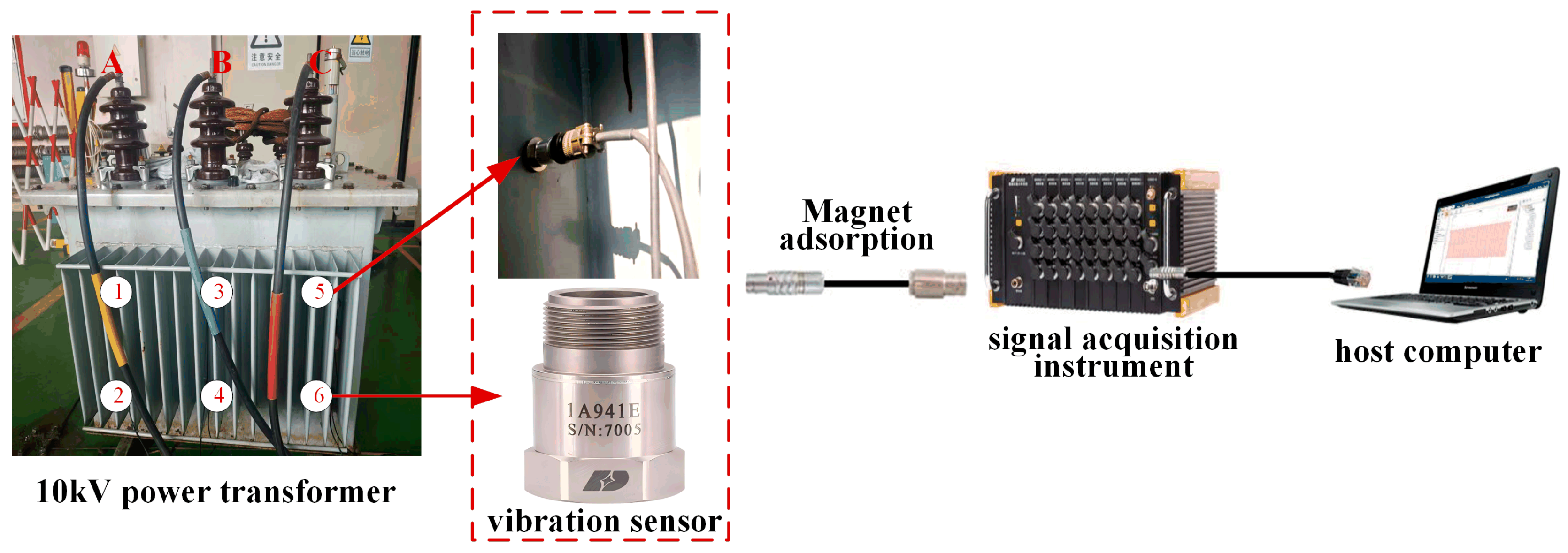
The test adopted the load short-circuit test; that is, the high-voltage side was pressurized and the low-voltage side’s three-phase winding was short-circuited. The test platform consisted of a 10 kV power transformer, vibration acceleration sensor, signal acquisition instrument, and host computer, as shown in Figure 1. In the figure, A, B, and C respectively represent the three phases (A, B, and C) of the transformer. The piezoelectric acceleration sensor of the model 1A941E was selected for measuring the vibration signal. It was evenly arranged in the front of the transformer box by magnetic attraction, and an acceleration sensor was pasted on the upper and lower 1/4 of the box surface corresponding to each phase winding, labels 1–6 indicated the six positions where sensors were installed. The signal acquisition instrument model was DH5902N, and the sampling frequency was 100 kHz.

With the aim of ensuring accurate fault identification under different load current conditions, a total of three load current conditions were set in the test: 90% $I_N$, 100% $I_N$, and 110% $I_N$, where $I_N$ is the rated load current of the high-voltage side’s winding. The vibration data collection duration for each condition was 10 s.

2.2. Transformer Winding Loose Fault Setting

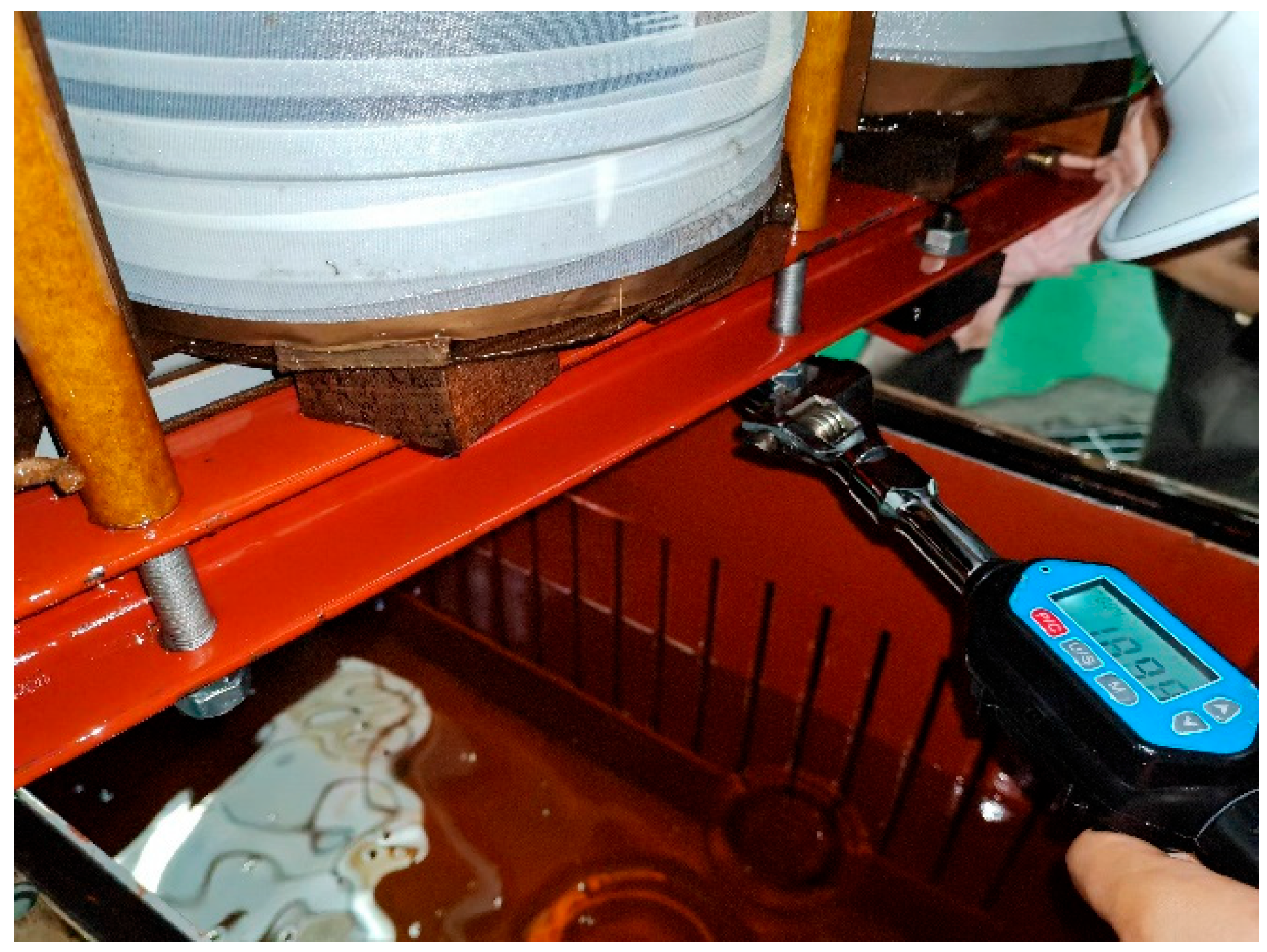
The internal windings of the 10 kV power transformer were tightened at both the top and bottom ends by the pull screw. As shown in Figure 2, the digital torque wrench was used to adjust the torque of the pull bolt to change the looseness of the winding.

According to the national standard, the calculation formula for the rated torque of bolts is presented below:

$$T=k{F}_{N}d$$

(1)

where T is the bolt torque, k is the bolt tightening coefficient, and the value range is 0.1~0.3; according to the general machining surface, the value of this test is 0.13. $F_N$ represents the rated preload of the bolt; in general, the rated preload is 80% of the yield strength of the bolt material. $d$ stands for the nominal diameter of the bolt (unit: mm). The following shows the formula used to compute the rated preload of bolts:

$$F_N=\left(0.5~0.7\right){\sigma }_s{A}_s$$

(2)

where ${\sigma }_s$ is the yield strength of the bolt material (unit: ${\mathrm{N}/\mathrm{mm}}^2$) and $A_s$ is the stress cross-sectional area (unit: ${\mathrm{mm}}^2$).

The test transformer’s winding upper and lower pressure plate pull bolt model was M12, with a strength grade of 4.6; nominal diameter: 12 mm; stress cross-sectional area: 84.3 ${\mathrm{mm}}^2$; yield strength: 240 ${\mathrm{N}/\mathrm{mm}}^2$. From Formula (1) and Formula (2), the formula of bolt torque can be obtained as follows [26]:

$$T={\displaystyle \frac{k\left(0.5~0.7\right){\sigma }_s{A}_{s}d}{1000}}$$

(3)

The rated torque range of the tension bolt at the end of the winding was calculated to be 16~22 $\mathrm{N}·\mathrm{m}$ by Formula (3). In the process of the winding loosening test, the digital torque wrench was used to measure the maximum rated torque of the winding to be 18 $\mathrm{N}·\mathrm{m}$, so as to determine the rated torque of the bolt at the end of the winding to be 18 $\mathrm{N}·\mathrm{m}$; that is, the transformer winding was not loose, expressed as 100% $F_N$.

Through the digital torque wrench, the torque of the bolts on the pull screw at the end of the three-phase winding of the transformer was adjusted in turn, to 13.5 $\mathrm{N}·\mathrm{m}$, 9 $\mathrm{N}·\mathrm{m}$, and 4.5 $\mathrm{N}·\mathrm{m}$, respectively. The three degrees of looseness of the transformer winding were defined as 75% $F_N$, 50% $F_N$, and 25% $F_N$, respectively. Therefore, when the value measured by the torque wrench is 13.5 $\mathrm{N}·\mathrm{m}$, it can be considered that the transformer winding has a loose fault, which is an abnormal state.

2.3. Vibration Signal Acquisition and Characteristic Analysis

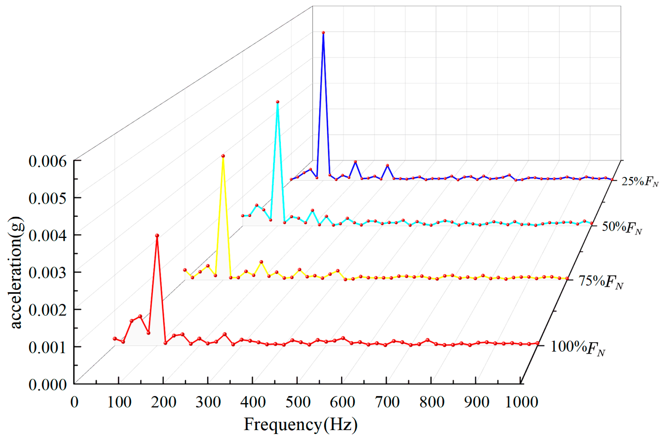
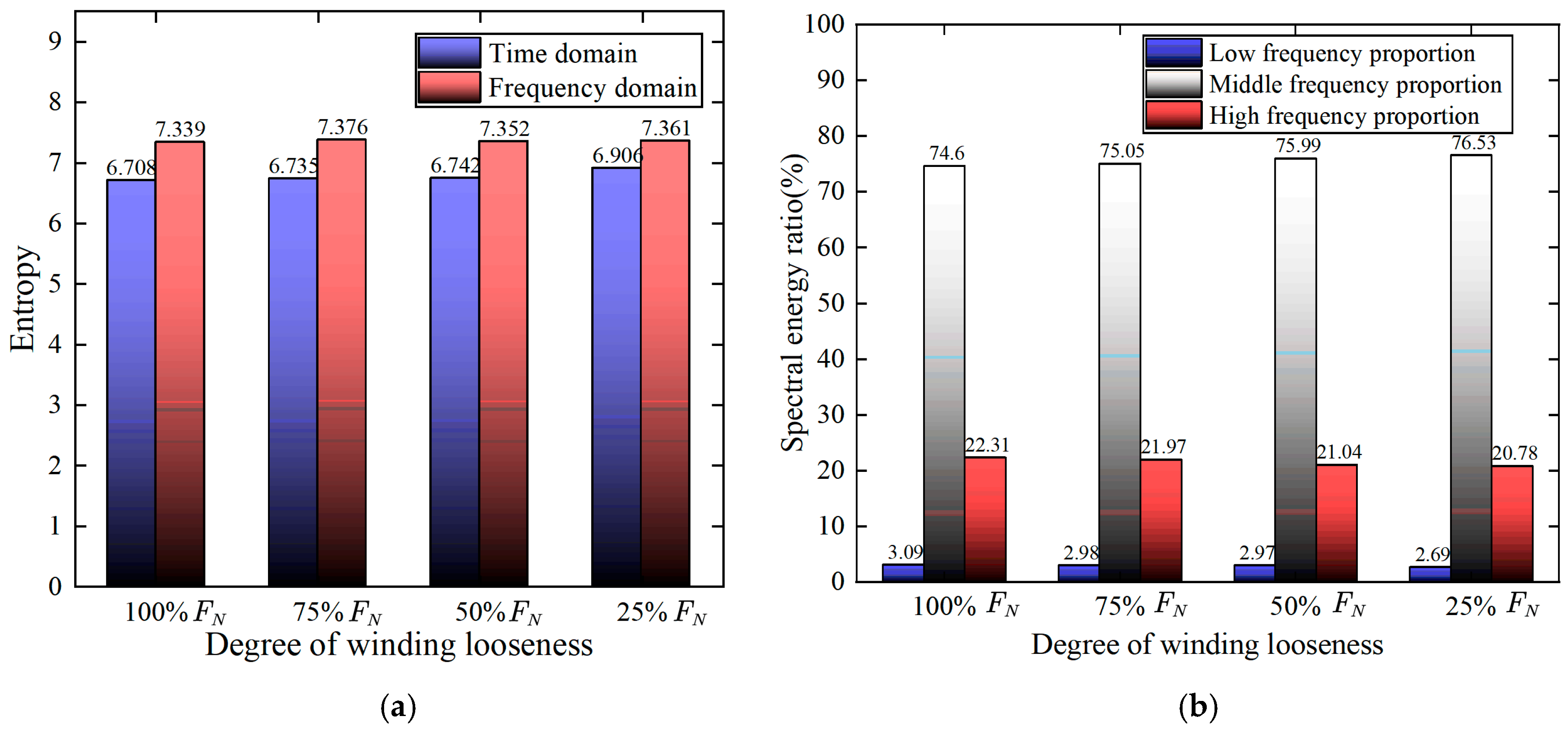
Under the operating condition of the transformer at its rated load, the vibration signal acquisition instrument was employed to collect the vibration signal waveforms of the transformer windings under five different degrees of looseness. Through time-domain analysis, the vibration signal showed no obvious regular change in amplitude. The time-domain signals were subjected to discrete Fourier transform to obtain the frequency-domain signals. The Figure 3 below shows the spectrum waterfall diagram of the three-phase windings of the transformer at Measuring Point 1 under different looseness fault states.

By analyzing the figure, it becomes clear that the fundamental frequency of the vibration signal for the transformer winding with different degrees of looseness is 100 Hz. The fundamental frequency amplitude increases with the increase in winding looseness.

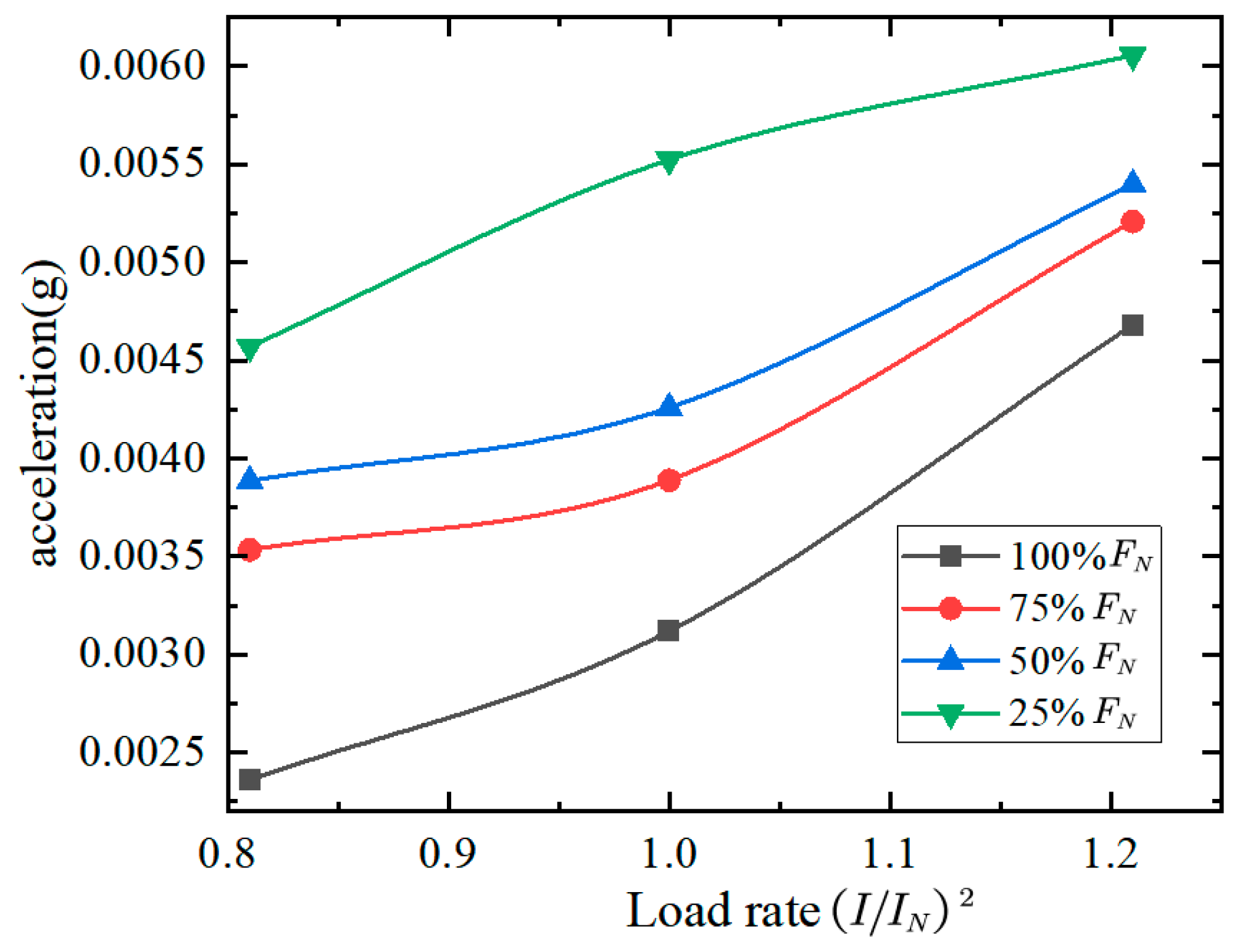
Ref. [27] indicates that the vibration acceleration of the transformer is essentially positively correlated with the square of the load current. By performing numerical fitting on the fundamental frequency amplitude of the vibration signal and the square of the load current when the transformer winding is in a normal condition and in a loose-fault state, the relationship curve is as shown in the figure.

From the analysis of Figure 4, it is evident that the amplitude of the fundamental frequency of the vibration signal increases with the square of the load current regardless of the normal operation of the transformer winding or the loosening fault. When the winding looseness fault occurs, the growth rate of the fundamental frequency amplitude and the load current change curve has a numerical relationship with the growth rate of the unloose winding.

To further extract the characteristic information of vibration signals before and after transformer winding loosening more comprehensively and achieve the accurate diagnosis and identification of transformer winding loosening faults, it is essential to encode the original vibration signal time series into two-dimensional images in the time domain and frequency domain. Before and after the transformer winding looseness fault occurs, there is a mapping relationship between the fundamental frequency amplitude of the vibration signal and the load current; that is, the vibration signal containing different load current conditions can also characterize the characteristic information before and after the winding fault. Therefore, this paper constructs the time–frequency-domain two-dimensional characteristic spectrum of the vibration containing different load conditions, so as to enrich the sample data of the vibration signal of the transformer winding and achieve the diagnosis and identification of the winding looseness fault under multiple working conditions.

3. Construction Method of Vibration Signal Characteristic Spectrum Under Transformer Winding Loosening Fault

3.1. Time-Domain Feature Map Construction Method Based on Relative Position Matrix

In terms of two-dimensional image coding technology, the relative position matrix method contains redundant feature information of the original time series, which makes the intra-class and inter-class similarity information of the converted two-dimensional image easier to capture [28]. The fundamental notion is to boost the convolutional neural network model’s ability to understand the sequence structure and extract features. This goal is accomplished through encoding the relative position connections between time-series elements. The specific steps of constructing two-dimensional feature maps by the relative position matrix are as follows:

(1)

Data normalization processing:

For the original time series, the normal distribution Z [29] is obtained by z-score normalization, as follows:

$$z_t={\displaystyle \frac{x_t-\mu }{\sigma }},t=1,2,\dots ,N$$

(4)

where $\mu$ indicates the average of X, while $\sigma$ indicates the standard deviation of X.

(2)

Data dimension reduction smoothing:

The piecewise aggregation approximation technique is employed to perform dimensionality reduction on the normalized time series. An appropriate value of the reduction factor k is chosen, and the dimension N is reduced to M, resulting in the creation of a new smooth time series.

$$\begin{array}{l}{\tilde{x}}_i=\{\begin{array}{l}\frac{1}{k}{\displaystyle \sum _{j=k^{\ast }\left(i-1\right)+1}^{k^{\ast }i}}{z}_j,i=1,2,\dots ,m,\lceil \frac{N}{k}\rceil -\lfloor \frac{N}{k}\rfloor =0\\ \{\begin{array}{l}\frac{1}{k}{\displaystyle \sum _{j=k^{\ast }\left(i-1\right)+1}^{k^{\ast }i}}{z}_j,i=1,2,\dots ,m-1\\ \frac{1}{N-k^{\ast }\left(m-1\right)}{\displaystyle \sum _{j=k^{\ast }\left(m-1\right)+1}^N}{z}_j,i=m\end{array},\lceil \frac{N}{k}\rceil -\lfloor \frac{N}{k}\rfloor >0\end{array}\\ m=\lceil \frac{N}{k}\rceil \end{array}$$

(5)

(3)

Relative position matrix generation:

The relative position between the two timestamps in the time domain is calculated, and the normalized vibration signal time series is converted into a two-dimensional matrix M, as shown below:

$$M=\left[\begin{array}{cccc}{\tilde{x}}_1-{\tilde{x}}_1& {\tilde{x}}_2-{\tilde{x}}_1& \dots & {\tilde{x}}_m-{\tilde{x}}_1\\ {\tilde{x}}_1-{\tilde{x}}_2& {\tilde{x}}_2-{\tilde{x}}_2& \dots & {\tilde{x}}_m-{\tilde{x}}_2\\ ⋮& ⋮& \ddots & ⋮\\ {\tilde{x}}_1-{\tilde{x}}_m& {\tilde{x}}_2-{\tilde{x}}_m& \dots & {\tilde{x}}_m-{\tilde{x}}_m\end{array}\right]$$

(6)

The minimum–maximum normalization approach is employed to transform the M matrix into a gray value matrix, and finally, the relative position matrix F [30] is obtained:

$$F={\displaystyle \frac{M-\min \left(M\right)}{\max \left(M\right)-\min \left(M\right)}}\times 255$$

(7)

(4)

Pseudo-color processing:

Through the mapping rules set in advance, each element in the feature matrix is regarded as an index value, and the intensity values of the corresponding R, G, and B are obtained in the Color Look-up Table according to the index value, so as to achieve the colorization of the gray matrix.

The flowchart of the two-dimensional map generated by the relative position matrix of the original vibration signal time series as shown in Figure 5:

As shown in Figure 6, the two-dimensional feature map of the vibration signal at Measuring Point 1 under the non-loosening state of the transformer winding is generated by the relative position matrix:

3.2. Construction of Frequency-Domain Feature Map Based on Gram Angle and Field

The spectrum distribution of transformer windings under different looseness fault states changes obviously, and the change in the fundamental frequency amplitude under each looseness state is positively correlated with the current. Therefore, the construction of frequency-domain feature maps under different load current conditions can more accurately reflect the characteristic information of different looseness faults of windings. The two-dimensional image generated by the Gram-angle field transformation [31] is capable of more effectively reflecting the characteristic information of the frequency-domain signal.

Before constructing the frequency-domain feature map, the original one-dimensional vibration signal needs to be transformed by Fourier transform to obtain the spectrum curve, and then the amplitude information corresponding to the frequency is saved in matrix form by Gram-angle field transform. Finally, the frequency-domain feature map is obtained by pseudo-color processing. The detailed procedures are presented below:

(1)

Complex modulation refines the spectrum:

The vibration signal frequency spectrum of the power transformer winding is predominantly concentrated in the range of 0~1000 Hz. In this experiment, the vibration signal acquisition rate is 100 Hz. After Fourier transform, the characteristic information contained in the low-frequency component cannot be clearly displayed in the spectrum. Therefore, it is necessary to perform complex modulation refinement operations to filter out the high-frequency part, so that the generated spectrum curve is concentrated within 0~1000 Hz [32]. The complex modulation refinement spectrum flow is shown in Figure 7.

As shown in Figure 7, the time series of the original vibration signal of the transformer $x_{in\left(n\right)}$ is transformed by Hilbert transform [33], and the complex analytical sequence ${\widehat{x}}_n$ is constructed, which is ${\widehat{x}}_n=\left\{a_1+j{b}_1,a_2+j{b}_2,\cdots ,a_n+j{b}_n\right\}$. Then, the complex analytic signal is modulated by the complex exponential signal to achieve the spectrum shift. The modulated signal undergoes low-pass filtering. This process removes the high-frequency components of the signal, leaving only the frequency signals within the 0~1000 Hz range. The filtered signal is resampled, and the sampling frequency is $f_s/D$. The resampled signal undergoes a discrete Fourier transform, followed by frequency adjustment and refinement before being output.

(2)

Data normalization processing:

The spectrum curve data after complex modulation refinement are normalized to make them range between [−1, 1], which can be directly used as the input of the cosine function. The detailed formula for normalized calculation is presented as follows:

$${\tilde{x}}_i={\displaystyle \frac{2\left(x_i-x_{\min }\right)}{x_{\max }-x_{\min }}}-1$$

(8)

(3)

Gram matrix generation:

The complex sequence after complex modulation refinement ${\widehat{x}}_n$ contains the amplitude and angle information of different frequency bands, and it does not need polar coordinate conversion. The obtained Gram-Angle Summation Field (GASF) matrix is as follows:

$$\mathit{GASF}=\left(\begin{array}{ccc}\cos \left({\theta }_1+{\theta }_1\right)& \dots & \cos \left({\theta }_1+{\theta }_n\right)\\ \dots & \cos \left({\theta }_i+{\theta }_i\right)& \dots \\ \cos \left({\theta }_n+{\theta }_1\right)& \dots & \cos \left({\theta }_n+{\theta }_n\right)\end{array}\right)$$

(9)

In this formula, ${\theta }_i$ is the angle value of the $i$-th sequence.

Carry out pseudo-color processing on the generated Gram matrix to obtain a two-dimensional characteristic graph in the frequency domain, and then compare it with the two-dimensional map generated without complex modulation refinement, as shown in Figure 8 below.

3.3. Quantitative Analysis of Time–Frequency-Domain Feature Images

In this section, a spectral mapping construction method is employed to generate time–frequency two-dimensional feature images for transformer windings with different degrees of looseness. Taking Measurement Point 1 as an example, quantitative analysis of the generated images is carried out from two dimensions: spectral energy and information entropy values.

Spectral energy analysis, grounded in Fourier transform, serves to quantify the energy distribution of images in the frequency domain and can reflect their high-frequency and low-frequency characteristics. Information entropy is used to measure the information content of an image or the uncertainty of pixel distribution. A higher entropy value indicates more complex image content and richer textures, while a lower entropy value signifies a simpler image. The calculation formula is as follows:

$$H=-{\displaystyle \sum _{i=0}^{L-1}p\left(i\right)}{\log }_{2}p\left(i\right)$$

(10)

where $p\left(i\right)$ represents the probability that the pixel value is $i$, and L is the range of pixel values.

This study defines low frequency as below 100 Hz, medium frequency within 100–500 Hz, and high frequency above 500 Hz. Information entropy values of time–frequency-domain feature maps and energy values of frequency-domain feature maps are computed for four transformer winding looseness faults (100% $F_N$, 75% $F_N$, 50% $F_N$, and 25% $F_N$). The resulting feature distributions are illustrated in the following figure.

Based on the analysis of Figure 9a, the information entropy values of frequency-domain spectra under four different loosening states of transformer windings exhibit no obvious regular changes, while the information entropy values of time-domain spectra increase with the aggravation of the loosening degree. According to the analysis of Figure 9b, as the winding loosening degree increases, the energy in the medium-frequency band rises, and the energies in both the high- and low-frequency bands decrease.

4. Construction of a Different Transformer Winding Loose Fault Diagnosis and Recognition Model Based on ConvNeXt

4.1. Limitations of Traditional Residual Convolutional Neural Networks

Lately, within the domain of ImageNet image classification and recognition, residual convolutional neural networks have introduced a residual block structure. This innovation effectively deals with the issues of gradient vanishing and gradient explosion in deep neural networks, thus improving the network performance to a certain extent [34]. However, with the progressive increase in network depth, the residual neural network needs strong GPU computing power, resulting in large resource consumption. When dealing with small-scale datasets, the strong expression ability of the residual neural network may cause the training outcomes to overfitting.

Given the deficiencies of the conventional residual neural network in the realm of image recognition, combined with the design direction and training strategy of vision transformers in the field of visual recognition, the parameters and structure of the existing ResNet50 model were optimized, and the improved ConvNeXt network model was obtained [35]. ConvNeXt uses Swin Transformer‘s sliding-window strategy to reuse the calculation results between each local area of the image [36], thereby reducing the amount of calculation. The model achieved excellent results in industrial machinery fault detection [37].

4.2. The Basic Structure of ConvNeXt Model

The ConvNeXt architecture encompasses five distinct variants: ConvNeXt-Tiny, ConvNeXt-Small, ConvNeXt-Base, ConvNeXt-Large, and ConvNeXt-XLarge. As delineated in

Table 2. Parameter comparison of ConvNeXt model variants.

Model Variants	Kernel Size	Layers	Parameter Count	Inference Time	FPS
Tiny	1 × 7 × 7	18	~29 M	~12 ms	~83 FPS
Small	1 × 7 × 7	24	~50 M	~20 ms	~50 FPS
Base	1 × 7 × 7	24	~89 M	~35 ms	~28 FPS
Large	1 × 7 × 7	24	~190 M	~70 ms	~14 FPS
XLarge	1 × 7 × 7	24	~290 M	~110 ms	~09 FPS

, ConvNeXt-Tiny features a streamlined design with fewer layers, while maintaining identical kernel dimensions to its counterparts. This lightweight configuration results in a parameter count just one-third that of ConvNeXt-Base, leading to reduced computational overheads and power consumption—qualities well suited for integration into fault diagnosis hardware. Moreover, its inference speed exceeds 80 FPS, fulfilling the latency requirements of real-time image classification tasks. Through comprehensive evaluation, ConvNeXt-Tiny was selected as the training model for this study.

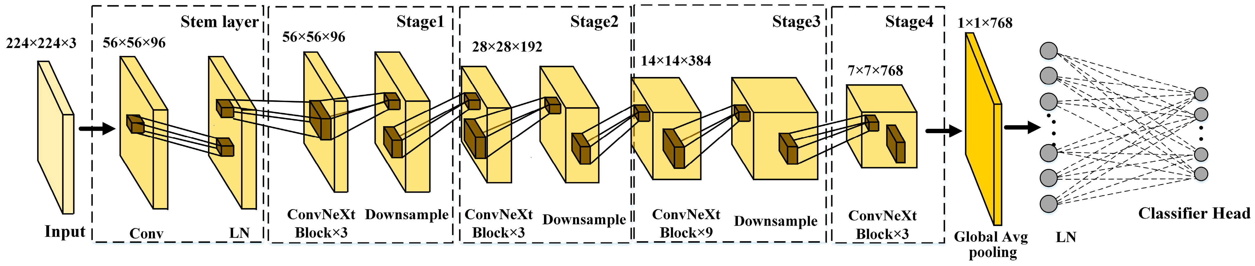
The ConvNeXt model draws on the design concept of transformer and adopts a hierarchical structure to divide the network into five modules. The model block diagram is shown in Figure 10. When the two-dimensional feature map enters the network, the Stem layer’s convolution operation conducts an initial extraction of feature information, and the layer normalization operation is utilized to lower the resolution. The ConvNeXt-Tiny model has four stages, each stage contains different numbers of ConvNeXt modules, and there are downsampling operations between the stages. The ConvNeXt blocks in stages 1 to 4 further extract and refine the feature maps output by the Stem layer, and they improve the expression ability of the feature maps by increasing the number of channels.

Finally, the feature map output from stage 4 is globally averaged in the spatial dimension, and the feature map of each channel is compressed into a scalar. Then, the feature vector is mapped to the number of categories through a fully connected layer, and the recognition accuracy corresponding to each category is provided as output.

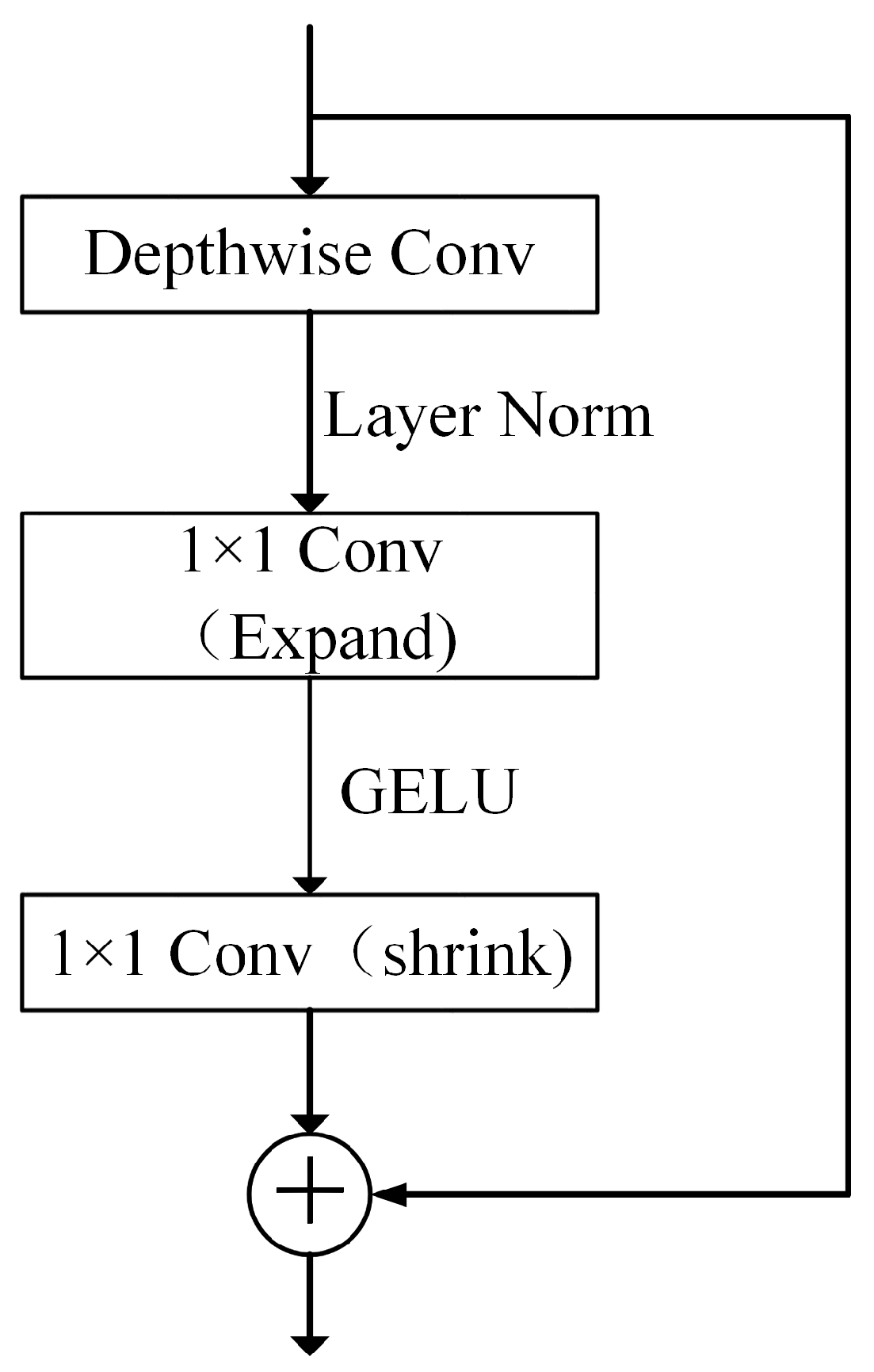
As shown in Figure 11, in contrast to the traditional residual module, the ConvNeXt module introduces depthwise convolution. Firstly, a 7 × 7 convolution kernel is used for each input channel to perform deep spatial convolution operation. After layer normalization, the influence of internal covariate offset is reduced, and the acceleration model converges. The 1 × 1 convolution is applied to fuse the output channels of the deep convolution, which significantly reduces the amount of calculation and maintains a good feature information extraction ability.

Gaussian Error Linear Unit (GELU) [38] was picked as the activation function, and the following is its formula:

$$GELU\left(x\right)=x·{\displaystyle \frac{1}{2}}\left(1+erf\left({\displaystyle \frac{x}{\sqrt{2}}}\right)\right)$$

(11)

In this formula, erf is the error function, defined as follows:

$$erf\left(x\right)={\displaystyle \frac{2}{\sqrt{2}}}{\displaystyle {\int }_0^x{e}^{-t^2}}dt$$

(12)

According to Formula (11), the GELU function is a nonlinear smoothing function, and the activation intensity is dynamically adjusted according to the distribution of input values. In the ConvNeXt module, the number of activation functions used is reduced, and only one activation function is added between two 1 × 1 convolutions. Finally, the input and output of the module are added, and the residual connection is helpful to alleviate the gradient disappearance, which makes it easier to train the model and enhance the model’s convergence.

The model training and visualization operations in this study were implemented using Python3.10. Code editing was performed via PyCharm 2022.3.3 (Professional Edition), the PyTorch framework was employed for deep learning and computer vision processing, and CUDA was utilized to drive GPU acceleration for image processing. Among them, the GPU version was an NVIDIA GeForce RTX 3070 Ti, and we used PyTorch version 2.5.1.

In terms of neural network training algorithm optimization, the AdamW [39] optimizer was used, and the relevant hyperparameters were set as follows: batch size = 16, max epoch = 100, and learning rate = 0.0001. The parameter settings of each module of the network are shown in

Table 3. Network module parameter settings.

Block	Kernel_Size	Stride
Stem layer	4 × 4	4
Stage1	Depthwise: 7 × 7	1
	Expand: 1 × 1	/
	Shrink: 1 × 1	/
Downsample layer	2 × 2	2

.

4.3. The Overall Process of Transformer Winding Looseness Fault Identification Based on the ConvNeXt Model

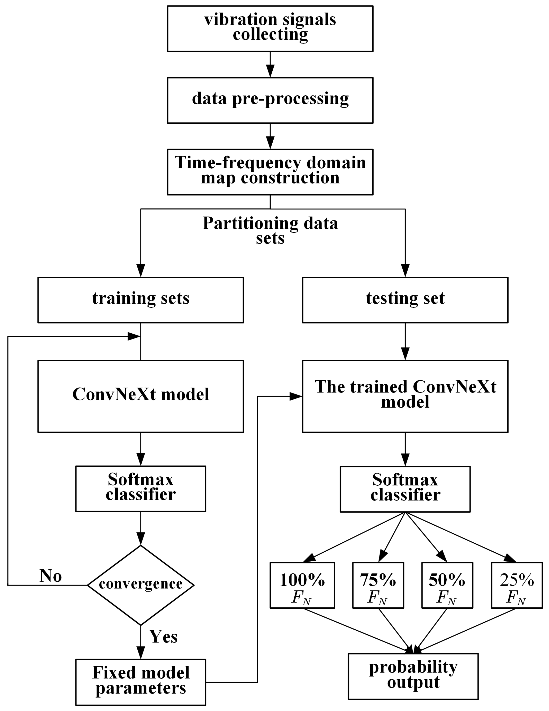
The process of diagnosing transformer winding looseness faults using the ConvNeXt model is illustrated in Figure 12 below.

(1) Vibration signal acquisition: The signal acquisition instrument is employed to collect the vibration signals of the box surface under various loose fault conditions of the three-phase winding of the transformer.

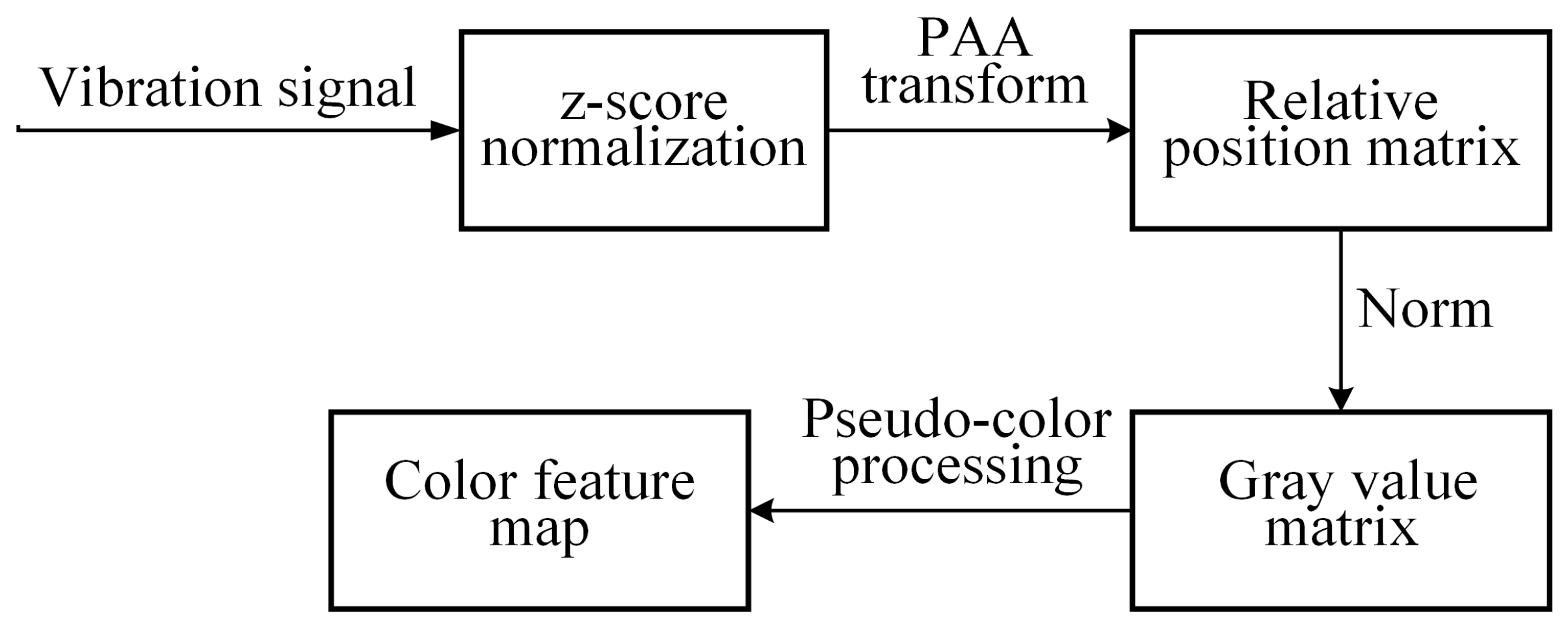
(2) Two-dimensional map library construction: For the collected original vibration signal time series, the relative position matrix is applied to produce the time-domain map, and the Gram-angle field is used to generate the frequency-domain feature map. Subsequently, a time-domain and frequency-domain feature map library for transformer winding looseness faults under various load current conditions is established.

(3) Model training: The time–frequency-domain feature map training set is fed into the constructed ConvNeXt model for training. Then, a softmax classifier is applied to yield the classification results, and the model’s training parameters are saved.

(4) Test set verification: The time–frequency characteristic spectrum test set is fed into the trained ConvNeXt model for testing, and the accuracy of transformer winding loose fault identification is diagnosed and identified.

5. Test Comparison and Analysis

5.1. Construction of Two-Dimensional Feature Map Data Samples

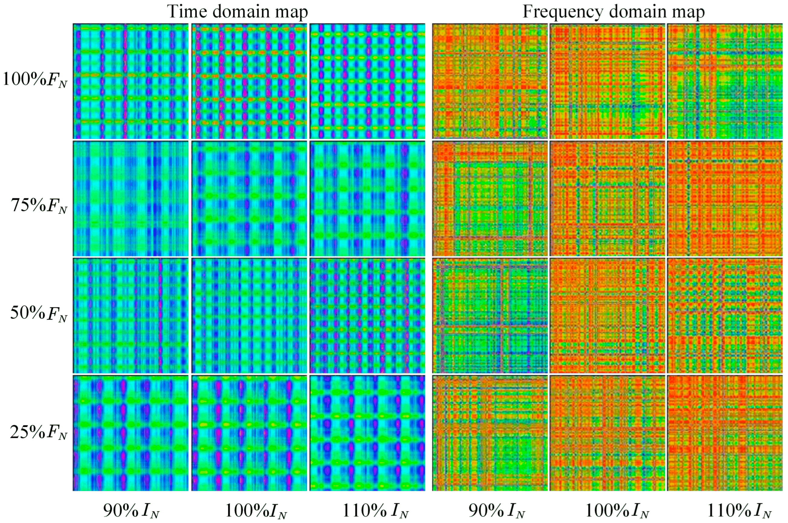
Before the image is transmitted to the ConvNeXt network for training, it is necessary to construct a sample library for the generated time–frequency-domain feature map. The vibrations of 100% $F_N$, 75% $F_N$, 50% $F_N$, and 25% $F_N$ loosening faults of the three-phase winding of the transformer are collected in the test; the signals of 90% $I_N$, 100% $I_N$, and 110% $I_N$ load conditions are collected for each loosening fault; and the time–frequency two-dimensional characteristic spectrum is constructed. In order to ensure that each image contains complete periodic feature information, the original vibration signal time series is processed by continuous slicing; each slice contains 4000 sampling points. The image sample set generated in this way contains three load current conditions under each loose fault state. The image samples generated by the winding loose fault signal corresponding to each measuring point are 11,964, and the size of each image sample is 224 × 224 × 3.

Figure 13 shows some image sample sets under different loose fault states of transformer windings.

5.2. Comparative Analysis of Transformer Winding Loose Fault Identification Under Different Load Current Conditions

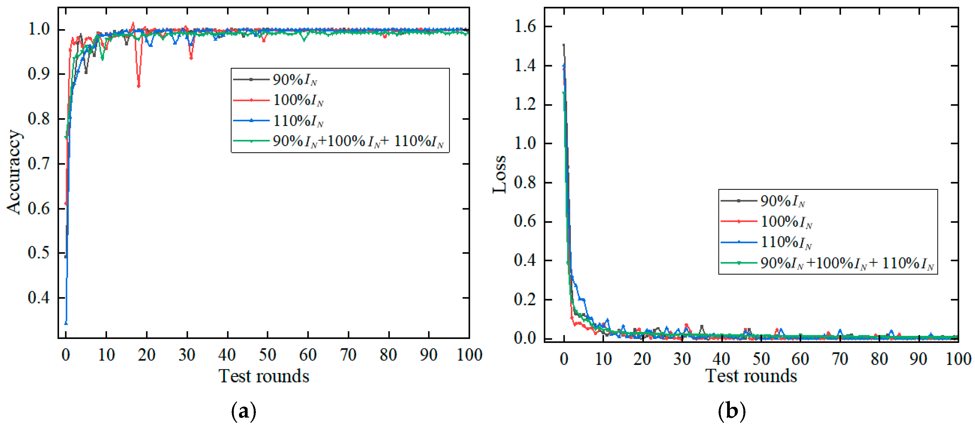
For the purpose of researching the precision of recognizing transformer winding looseness faults in different load situations, the time–frequency-domain feature maps generated under three load conditions of 90% $I_N$, 100% $I_N$, and 110% $I_N$ of the transformer were input into ConvNeXt for training. A total of 3988 images were generated under each load current condition. The samples under the load condition were partitioned into a training set and test set at a ratio of 5 to 1, and there were 100 training rounds. Taking Measuring Point 1 as an example, the change curves of recognition accuracy and loss value of the test set were obtained as shown in Figure 14 below, the recognition accuracy under different load conditions is shown in

Table 4. Recognition accuracy under different load conditions.

Different Load Conditions	The 100th Round of Recognition Accuracy (%)
$90\% I_N$	99.25
$100\% I_N$	100
$110\% I_N$	100
$90\% I_N+100\% I_N+110\% I_N$	99.54

.

From the training correlation curves of transformer winding looseness identification under different load current conditions, it is evident that regarding the identification accuracy of the test set, the three load conditions of 90% $I_N$, 100% $I_N$, and 110% $I_N$ all reached more than 99% after the 50th round of testing, and the accuracy of test set identification under the mixture of the three load conditions also reached 99.54%. In terms of the convergence performance of the loss function, the convergence performance of the test set under the three load current conditions had a significant advantage, and the loss value tended toward 0, while the other three load current conditions had different degrees of fluctuation in the loss value when they were trained separately.

In summary, the two-dimensional images under three load conditions of 90% $I_N$, 100% $I_N$, and 110% $I_N$ not only enriched the dataset in the identification of transformer winding looseness faults but also achieved very high recognition accuracy and good convergence.

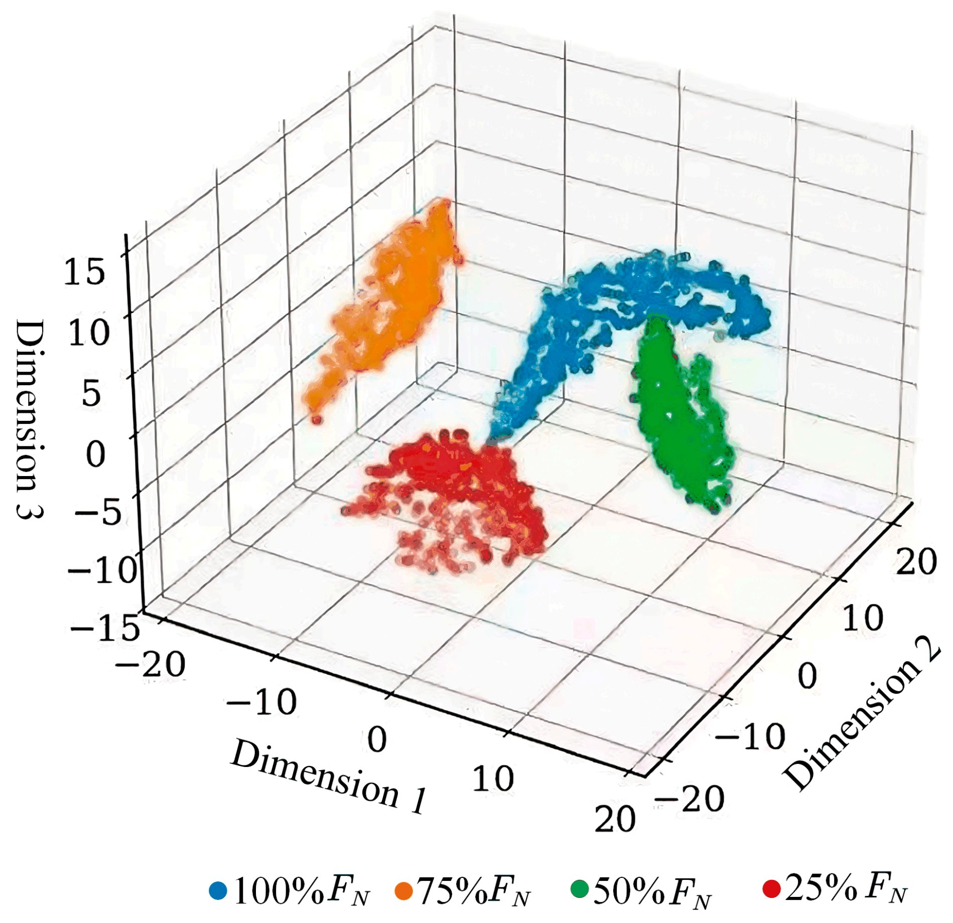
The T-distributed Stochastic Neighbor Embedding (T-SNE) dimension reduction processing [40] was performed on the fault classification and recognition feature quantity at Measuring Point 1, and the visual 3D effect diagram shown below was obtained. As shown in Figure 15, it can be seen that each loose fault classification shows good independence, of which the 75% $F_N$ loose fault classification effect is better.

To verify the sensitivity of the recognition accuracy of the ConvNeXt model to the number of image samples, 80%, 60%, and 50% of the spectrum samples from Measurement Point 1 were extracted and input into the model for training and recognition, with the number of training epochs set to 100. The distribution of the recognition accuracy of the test set samples at the 100th epoch is shown in

Table 5. The distribution of model recognition accuracy under different sample numbers.

The Proportion of Image Samples (%)	The 100th Round of Recognition Accuracy (%)
100	99.54
80	96.77
60	89.31
50	85.33

below.

Analysis of the table reveals that when the number of spectrum samples drops to 80%, the 100th round of recognition accuracy of Measurement Point 1 decreases by nearly 3 percentage points. When the sample quantity is halved, the 100th round of recognition accuracy falls to 85.33%. Thus, the number of samples is one of the key factors influencing the recognition accuracy of the ConvNeXt model; the more sufficient the samples, the richer the fault feature information extracted by the model.

5.3. Comparative Analysis of Transformer Winding Loose Fault Identification Under Different Measuring Points

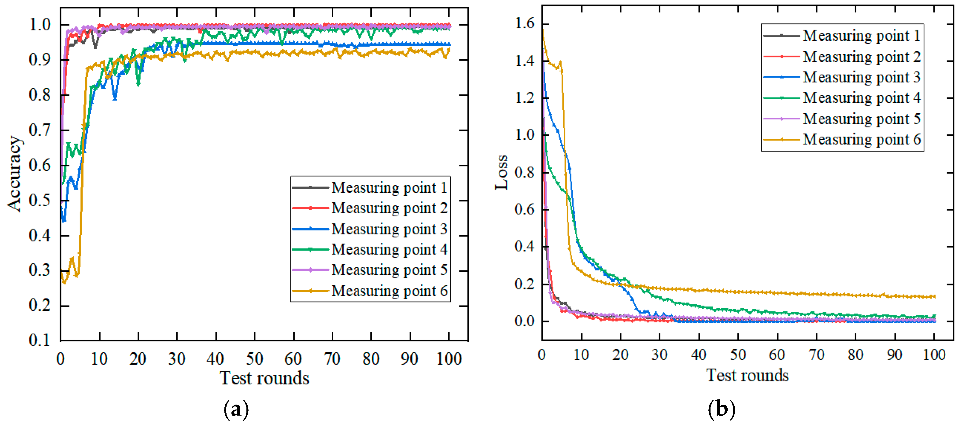
In this section, the two-dimensional spectra of different winding loose fault states, corresponding to six measuring points, were trained and identified. Each measuring point contained vibration data in four states of 100% $F_N$, 75% $F_N$, 50% $F_N$, and 25% $F_N$, with a total of 71,784 images. The samples included in the measuring point were partitioned into a training set and test set at a ratio of 5 to 1. The data samples were fed into the ConvNeXt model for training, and the number of training rounds was set to 100. The change curves of the recognition accuracy rate and the loss value of the test set after training for each measuring point were obtained, as shown in Figure 16 below:

Comprehensive analysis of the test set recognition accuracy and loss value transformation curve in the figure shows that the convergence of Measuring Points 1, 2, and 5 is the best in the recognition process. When the testing reaches the 10th round, the recognition accuracy of Measuring Points 1, 2, and 5 tends to be stable, reaching 97.9%, 100%, and 97.0%, respectively. When the testing reaches 50 rounds, the loss function of Measuring Points 3 and 4 effectively reaches the convergence state, and the recognition accuracy is 94.7% and 96.9%, respectively. The convergence of the loss function at six measuring points is poor, and the loss value is 0.11. After 100 rounds of recognition on the test set, the accuracy rate reaches 93.7%, which has a relatively good classification effect.

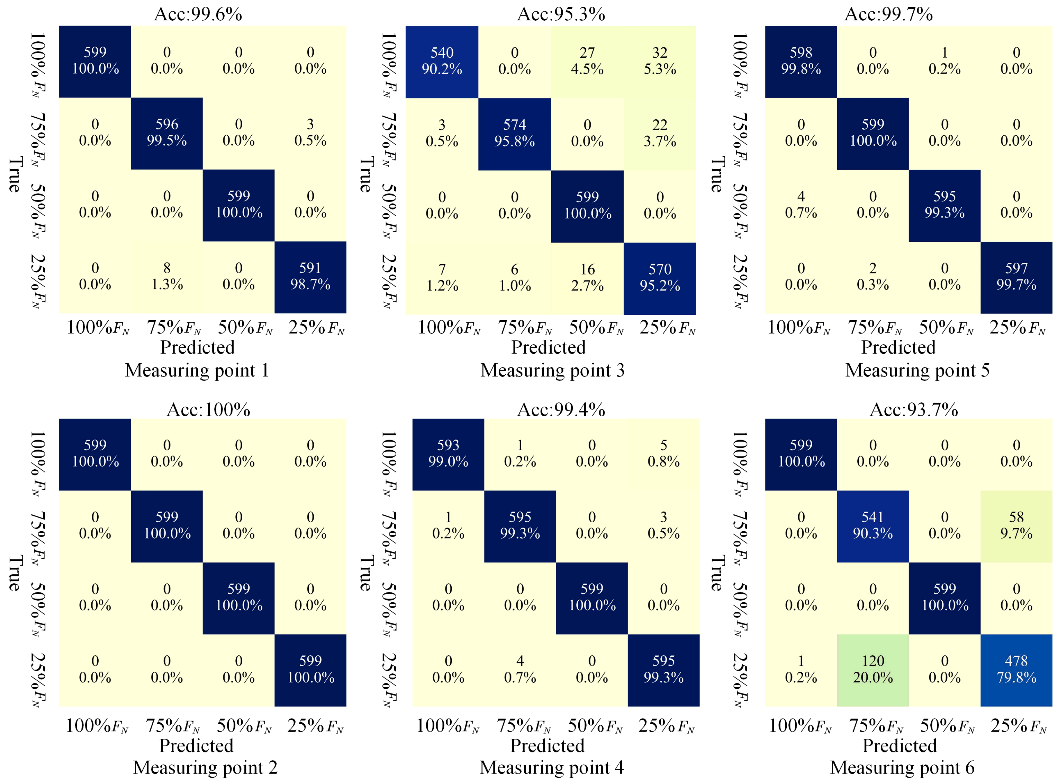
Figure 17 shows the confusion matrix under the 100th round of identification of the test set of six measuring points.

Based on the confusion matrix, the classification precision, recall rate, and F1-scores for each measurement point were calculated, yielding the evaluation indicators shown in

Table 6. Classification evaluation index of different measuring points.

Measuring Point	Looseness Grade	Precision (%)	Recall (%)	F1-Score (%)
1	100% $F_N$	100	100	100
	75% $F_N$	100	99.5	99.7
	50% $F_N$	100	100	100
	25% $F_N$	99.5	98.7	99.1
2	100% $F_N$	100	100	100
	75% $F_N$	100	100	100
	50% $F_N$	100	100	100
	25% $F_N$	100	100	100
3	100% $F_N$	98.1	90.2	93.9
	75% $F_N$	98.9	95.8	97.3
	50% $F_N$	93.3	100	96.5
	25% $F_N$	91.3	95.2	93.2
4	100% $F_N$	99.8	99	99.4
	100% $F_N$	99.1	99.3	99.2
	75% $F_N$	100	100	100
	50% $F_N$	98.6	99.3	98.9
5	100% $F_N$	99.3	99.8	99.5
	75% $F_N$	99.6	100	99.8
	50% $F_N$	99.8	99.3	99.5
	25% $F_N$	100	99.7	99.8
6	100% $F_N$	99.8	100	99.9
	75% $F_N$	81.8	90.3	85.8
	50% $F_N$	100	100	100
	25% $F_N$	89.1	79.8	84.2

. A comprehensive analysis revealed that Measurement Points 1, 2, 4, and 5 exhibited remarkably high average recognition accuracy, demonstrating the exceptional classification capability of the ConvNeXt model. Notably, the test set images at Measurement Point 2 achieved 100% $F_N$ correct classification, representing a perfect performance. For Measurement Point 3, the 75% $F_N$ fault condition showed significant recognition advantages, with an F1-score of 97.3%, while the recall rate for the 100% $F_N$ fault condition was poor. At Measurement Point 6, the datasets under 75% $F_N$ and 25% $F_N$ fault conditions suffered severe classification confusion, with F1-scores of 85.8% and 84.2%, respectively—significantly worse than the other measurement points in terms of overall recognition performance.

From the above-mentioned analysis, it is evident that the model recognition accuracy of the six measuring points on the surface of the transformer box is generally high, and the average recognition accuracy of all measuring points is 97.9%, which can essentially reflect the recognition effect under the three-phase loosening fault of the transformer winding.

5.4. Model Robustness Verification

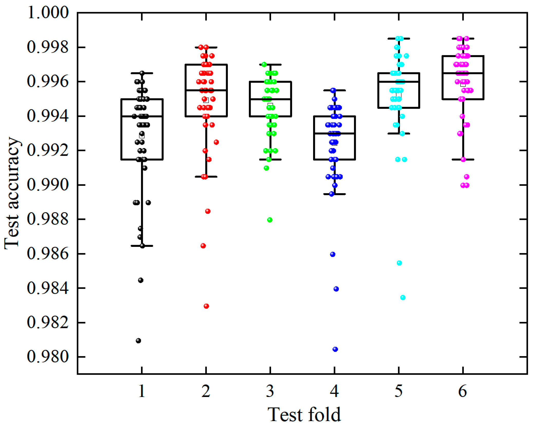
To mitigate overfitting caused by fixed training–test splits and ensure the robustness of the ConvNeXt model, this section incorporated a 6-fold cross-validation pipeline during training. The dataset was repeatedly partitioned and trained across six iterations, with each iteration validated on a distinct subset. Two-dimensional spectra corresponding to different winding looseness fault states at six measurement points were trained individually. For instance, taking Measurement Point 1 as a case study, the boxplot of recognition accuracy for each fold after the 50th training epoch was generated.

Analysis of Figure 18 indicates that the six-fold test sets exhibit generally excellent overall recognition accuracy, with all boxplot boxes remaining narrow—evidence of the model’s robust recognition stability. Subsequently, the average recognition accuracy for each fold across the six measurement points was calculated, alongside the standard deviation of the six-fold training outcomes. The standard deviation formula is as follows:

$$\sigma =\sqrt{{\displaystyle \frac{{\displaystyle \sum _{i=1}^n{\left(x_i-\mu \right)}^2}}{n}}}$$

(13)

where $\sigma$ denotes the volatility, $\mu$ signifies the average value of the data, and $n$ indicates the quantity of data.

Analysis of

Table 7. The training recognition accuracy and standard deviation distribution of each measuring point.

Measuring Point	Average Recognition Accuracy	Standard Deviation
1	99.427	0.00207
2	99.999	0.00021
3	95.439	0.00558
4	98.291	0.00177
5	99.523	0.00059
6	92.529	0.00731

shows that, after six-fold cross-training, the average recognition accuracy of each measurement point dataset exhibits no significant change compared to the training results in Section 5.3, and the standard deviation is also minimal. This verifies that the ConvNeXt model has a certain degree of robustness in the division of the test set and validation set.

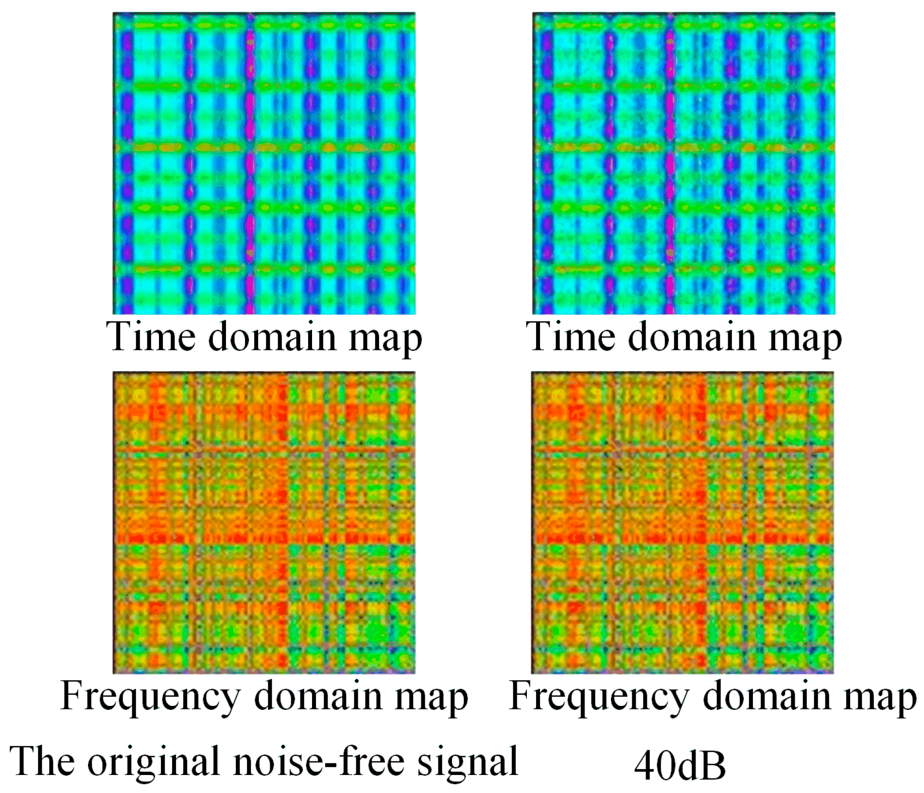
To validate the ConvNeXt model’s robustness against noise, the following section classifies noisy vibration signals. Gaussian white noise with specified power was added to the original signals to generate samples at varying signal-to-noise ratios (SNRs). These noisy signals were then converted into time–frequency-domain 2D feature maps using the spectrum construction method. The Figure 19 below compares the 2D spectrum of the original signal with that of a signal processed at 40 dB SNR.

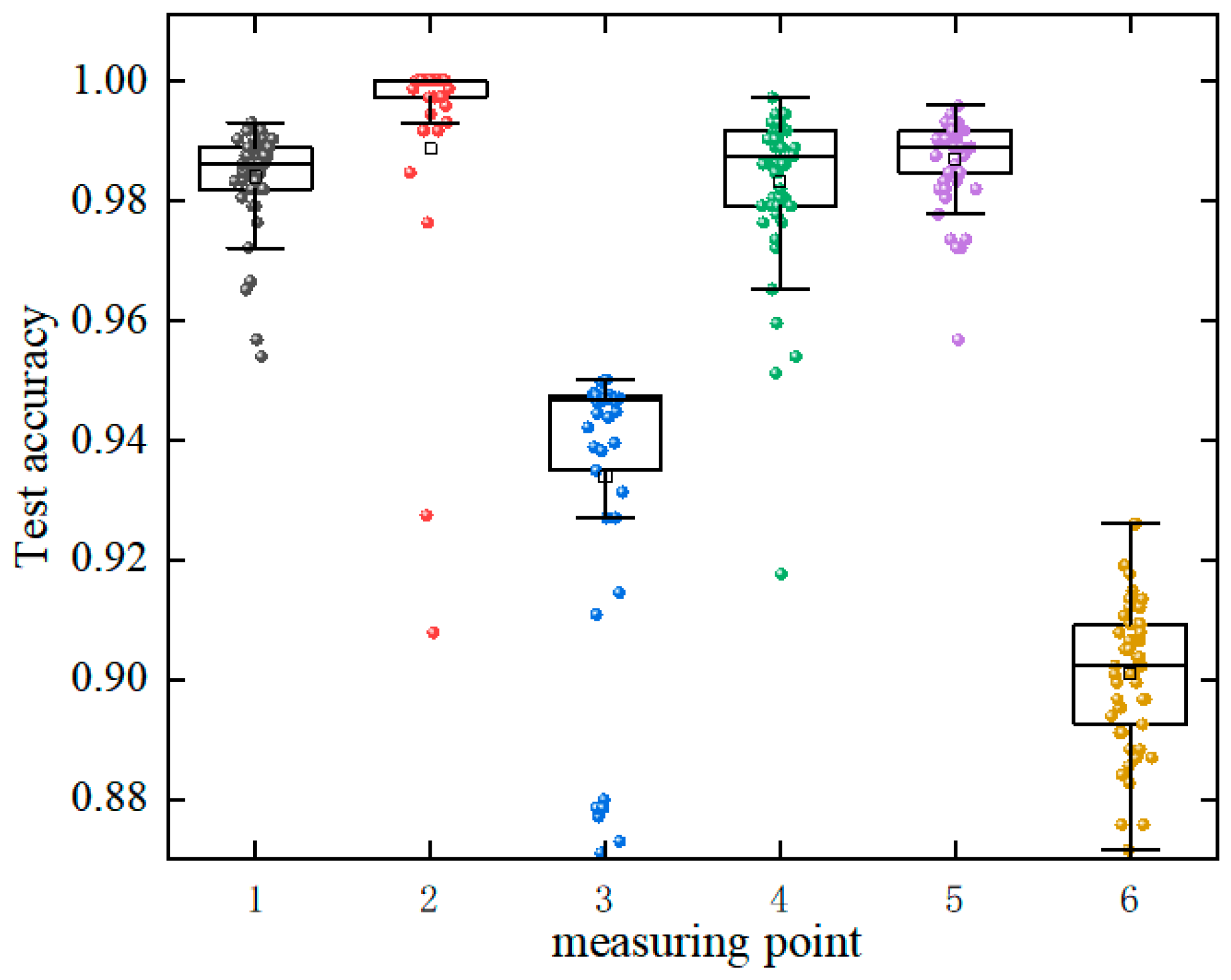
The spectral dataset with an SNR of 40 dB was fed into the ConvNeXt model for training, yielding a boxplot of recognition accuracies for the six measurement points’ test sets after the 50th training epoch.

Analysis of Figure 20 reveals that Measurement Points 2, 4, and 5 exhibit higher box positions, higher medians, and lower dispersion—indicative of consistently excellent and stable test accuracy. In contrast, Points 3 and 6 show lower box positions and greater dispersion, leading to lower overall accuracy with pronounced fluctuations. Notably, after introducing Gaussian noise, the recognition accuracy of each measurement point dataset showed no significant change compared to the noise-free datasets.

The SNR values were sequentially varied to 40 dB, 30 dB, 20 dB, and 10 dB. Vibration spectra corresponding to different SNRs were fed into the ConvNeXt model for training and recognition, after which the average recognition accuracy across the six measurement points was calculated. Table 7 presents the model’s average recognition accuracy and standard deviation distribution under varying SNR conditions.

Analysis of

Table 8. Average recognition accuracy and sample difference under different signal-to-noise ratios.

SNR	Average Recognition Accuracy
raw vibration signal	97.9
40 dB	97.9
30 dB	97.9
20 dB	96.3
10 dB	95.7

demonstrates that, when the SNR exceeds 30 dB, the classification performance of the condition recognition model remains unaffected. Conversely, as the SNR drops below 30 dB, although a slight decrease in accuracy is observed, the recognition rate still maintains a relatively high level. This indicates that the ConvNeXt model exhibits notable robustness against noise interference.

5.5. Comparative Analysis of the Recognition Effect of Different Training Models

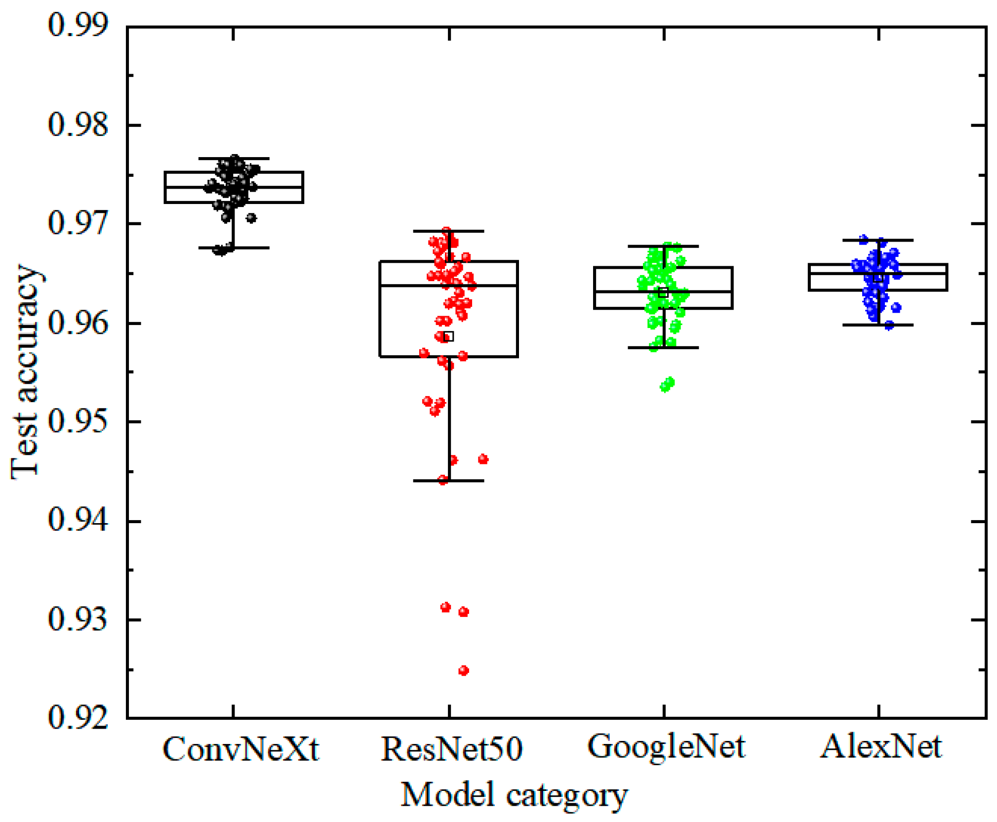
To validate the superiority of the ConvNeXt model, this study compared the recognition performance of four models: ConvNeXt, ResNet50, GoogLeNet, and AlexNet. A boxplot of recognition accuracies after the 50th training epoch was plotted, as shown in Figure 21 below:

According to the analysis of Figure 21, The ConvNeXt model demonstrates marked superiority in recognition accuracy over other models, with lower dispersion and concentrated distribution. By contrast, the ResNet50 model exhibits higher dispersion in accuracy, occasionally showing notably lower values, indicating inferior stability to ConvNeXt. The GoogLeNet model features better accuracy concentration than ResNet50, yet its overall recognition performance remains inferior to that of ConvNeXt. Although AlexNet shows moderate dispersion, both its central tendency and concentration range lag behind those of other models. The average recognition accuracy and standard deviation of the four models after the 50th test epoch are statistically analyzed below, as tabulated in

Table 9. Different models’ recognition accuracy and volatility.

Recognition Model	Identification Accuracy (%)	Standard Deviation
ConvNeXt	97.9	0.0020
ResNet50	96.7	0.0110
GoogLeNet	95.3	0.0042
AlexNet	96.1	0.0005

:

From the comparative analysis of Table 9, it is clear that the ConvNeXt model has a distinct advantage in the accuracy of transformer winding looseness recognition, which is 1.2% higher than that of the traditional ResNet50 model. After the 50th test epoch, the standard deviation of recognition accuracy for ConvNeXt is only 0.002. While AlexNet exhibits the smallest standard deviation, its average recognition accuracy remains relatively low. Therefore, the ConvNeXt model has a significant effect in the diagnosis and identification of transformer winding looseness faults.

6. Conclusions

In this study, the time–frequency-domain feature map library of winding looseness faults under different transformer load current conditions was constructed by using the relative position matrix and Gram angle and field. The fault diagnosis and identification model of transformer winding looseness relying on feature maps and ConvNeXt was built, and the experimental verification was carried out. The following conclusions were reached:

(1) The time–frequency two-dimensional feature map library under three load currents of 90% $I_N$, 100% $I_N$, and 110% $I_N$ was constructed, and the fault recognition accuracy and convergence of the test set reached the performance under the single load current condition. The recognition rate of the test set of Measuring Point 1 was as high as 99.54%; it provided sample data for the diagnosis and identification of transformer looseness faults across various load conditions, and it improved the adaptability of the model to the diagnosis of transformer winding looseness faults with various load conditions.

(2) The recognition accuracy of the ConvNeXt looseness fault model corresponding to the six measuring points on the measuring surface of the transformer box was generally high, and the average recognition accuracy of all measuring points was 97.9%.

(3) The ConvNeXt model improved the accuracy of transformer winding looseness fault identification by 1.2% compared with the traditional ResNet50, solving the overfitting problem of traditional model training to a certain extent, and showed significant advantages in fault classification effect.

In summary, the transformer winding looseness fault identification model proposed in this paper, integrating feature spectrograms and ConvNeXt, demonstrates remarkable advantages in both recognition efficiency and robustness. This model not only provides technical support for mechanical fault diagnosis of transformer windings in operational substations but also lays a theoretical foundation for the research on fault diagnosis devices.

This study still has certain limitations. First, only a single type of power transformer was used in the experiment, which cannot fully reflect the general law of transformer winding looseness. Second, only a single sensor arrangement scheme was used in the experiment, which cannot completely capture the characteristic information of transformer winding vibration. Third, image recognition for transformer winding looseness faults generally only identifies the occurrence of such faults, struggling to precisely locate the internal fault positions—such as the specific turn layer of a phase coil. Therefore, this paper proposes the following solutions:

1. Measure the vibration data of different types of transformer windings under faults to enrich the fault spectrum database of transformer winding looseness.

2. Increase the number of sensors, and uniformly arrange sensors on the top and sides of the transformer tank to fully collect the vibration signals of the transformer.

3. Position fiber-optic sensors between the transformer winding pancakes to monitor stress variations, generate spectrograms from tank surface vibration signals to detect faults, and use fiber-optic sensor data to localize faults. Establish a correlation model between the two sensor datasets to enable the precise localization of winding looseness faults in subsequent experiments using only vibration sensor data.