Implementation of a Non-Intrusive Primal–Dual Method with 2D-3D-Coupled Models for the Analysis of a DCB Test with Cohesive Zones

Abstract

This study explores a global–local non-intrusive computational strategy to address problems in computational mechanics, specifically applied to a double cantilever beam (DCB) with cohesive interfaces. The method aims to reduce computational requirements while maintaining accuracy. The DCB, representing two plates connected by a cohesive zone simulating delamination, was modeled with a 3D representation using the cohesive zone method for crack propagation. Different mesh configurations were tested to evaluate the strategy’s effectiveness. The results showed that the global–local strategy successfully provided solutions that were comparable to monolithic models. Mesh size had a significant impact on the results, but even with a simplified local model that did not fully represent the plate thickness, the structural deformation and crack displacement were accurately captured. The interface near the study area influenced the stress distribution. Although effective, the strategy requires careful mesh selection due to its sensitivity to mesh size. Future research could optimize mesh configurations, expand the strategy to other structures, and explore the use of orthotropic materials. This research introduces a computational approach that reduces costs while simulating delamination and crack propagation, highlighting the importance of mesh configuration for real-world applications.

1. Introduction

Cross-laminated timber (CLT) has emerged as a viable structural material in modern construction due to its favorable mechanical properties, ease of prefabrication, and suitability for large-scale applications. Its layered configuration, provides enhanced stiffness and dimensional stability, making it particularly attractive for multi-story buildings and modular construction systems.

CLT is composed of an odd number of orthogonally arranged timber layers bonded with adhesives, providing high load-bearing capacity and structural stability. Its modular design allows for prefabrication and rapid on-site assembly, enhancing construction efficiency while reducing material waste and energy consumption.

To ensure the safe and efficient use of CLT in structural applications, it is essential to understand its failure mechanisms. Therefore, computational simulations have become indispensable tools in this context, enabling virtual testing under various loading and degradation scenarios, while extensive research exists for composite materials like fiber-reinforced plastics, the study of fracture resistance in CLT, especially under nonlinear phenomena such as buckling, remains limited. Nevertheless, methodologies such as multisurface failure criteria [1,2], lattice models [3], cohesive damage models [4,5,6,7], finite fracture mechanics concepts [8,9], and the extended finite element method (XFEM) [10,11] offer valuable frameworks that can be adapted to wooden materials.

Rolling shear failure, a critical phenomenon in CLT panels, has been previously investigated with good correlation between experimental and numerical results [5,12,13]. Additional studies have addressed the influence of shear deformation, number of layers, and geometric features on buckling behavior [14,15]. However, the coupled effect of buckling and crack propagation, particularly delamination, has received little attention in the literature.

One of the main challenges in modeling this interaction is the disparity in scale: buckling manifests at the structural level, while delamination occurs at the material level. Accurately capturing these multi-scale phenomena requires fine-meshed, high-resolution models and significant computational resources. This complexity calls for advanced strategies such as domain decomposition and global–local modeling.

Cohesive zone modeling (CZM) has advanced significantly in recent years, offering reliable tools for simulating fracture in heterogeneous materials. Research has focused on providing a foundation for consistent energy dissipation in fracture simulations [16], mixed-mode fracture [17], Mode I delamination coupled with fiber bridging [18], arbitrary or complex crack propagation paths [19,20], rate-dependent cohesive laws [21], adaptive meshing [22], parameter identification [23,24], integration with multiscale and non-intrusive methods [25,26,27,28], combining cohesive elements with XFEM [29], the prediction of fatigue life of adhesive joints for automotive applications [30], and temperature-dependent material properties [31], among others. These developments have improved the capacity to simulate complex failure mechanisms efficiently and accurately.

This study aims to evaluate the applicability of a primal–dual global–local strategy [32,33] to simulate crack growth in a double-cantilever beam (DCB) test. To mitigate the numerical complexities associated with the anisotropic behavior of CLT, the analysis is initially implemented using an isotropic material, allowing for a more robust evaluation of the method’s performance and convergence behavior.

Is important to mention that in engineering practice, the modeling of CLT or any other wall type elements are made using 2D shell elements, with rotational and translational degrees of freedom per node. Therefore, to capture the correct behavior of the adhesive analysis using CZM or another interface model technique, a coupled analysis between 2D shell elements and 3D complex nonlinear behavior must be considered. In consequence, the proposed strategy integrates a global plate model with a finely meshed 3D submodel enriched with cohesive elements, enabling the representation of crack propagation while maintaining computational efficiency. Prior implementations have demonstrated the potential of this approach in modeling plasticity and fracture [34,35,36], and this work extends its application to fracture analysis under a multiscale framework using cohesive zone modeling. In particular, the present study focuses on assessing how the selection of the local model, considering both its discretization and the extent of the structural domain it represents, affects the accuracy and reliability of the global–local simulation results.

2. Global–Local Problem Formulation

2.1. Reference Problem

Considering an elastic body with a small displacement formulation, the differential eq. governing the system can be described using the following equation:

$$\begin{array}{cc}\hfill -\nabla ·\sigma \left(u\right)& =f\mathrm{in}\mathrm{\Omega }\hfill \end{array}$$

(1)

$$\begin{array}{cc}\hfill \sigma \left(u\right)& =\lambda \mathrm{tr}\left(ϵ\right(u\left)\right)I+2\mu ϵ\left(u\right)\hfill \end{array}$$

(2)

$$\begin{array}{cc}\hfill ϵ\left(u\right)& ={\displaystyle \frac{1}{2}}\left(\nabla u+{(\nabla u)}^T\right)\hfill \end{array}$$

(3)

where $\sigma$ is the Cauchy tensor, f is the applied body force, $\lambda$ and $\mu$ are the Lamé elasticity parameters of the material in the domain $\mathrm{\Omega }$, u is the displacement field of the problem, $ϵ$ is the strain tensor, and I is the identity tensor.

Using the weak formulation of the problem and multiplying it by a test function v, the equilibrium equation is presented as follows:

$${\int }_{\mathrm{\Omega }}\sigma :\nabla vs.\mathrm{d}x={\int }_{\mathrm{\Omega }}f·vs.\mathrm{d}x+{\int }_{\partial {\mathrm{\Omega }}_T}T·vs.\mathrm{d}s.$$

(4)

where T is the stress tensor at the boundary $\partial {\mathrm{\Omega }}_T$ of the problem analyzed. Applying the boundary conditions to the problem and considering that $\mathrm{\Omega }$ is noted as the reference domain ${\mathrm{\Omega }}_R$, the mechanical problem to be solved can be described by the following equations.

$$\mathrm{Find}u\in V\left({\mathrm{\Omega }}_R\right),a_R(u,v)=l_R\left(v\right),\forall vs.\in V_0\left({\mathrm{\Omega }}_R\right)$$

(5)

The admissible space for the displacements is defined as:

$$V\left({\mathrm{\Omega }}_R\right)=\{V\in H_1\left({\mathrm{\Omega }}_R\right)v=u_d\mathrm{on}{\partial }_u{\mathrm{\Omega }}_R\}$$

(6)

where $a_R$ is the bilinear operator related to the equilibrium of the structure and $l_R$ are the Neumann boundary conditions. For Dirichlet boundary conditions, these are within the admissible displacement space $V\left({\mathrm{\Omega }}_R\right)$.

2.2. Implemented Non-Intrusive Method

The nonlinear reference structure ${\mathrm{\Omega }}_R$, representing the DCB test, is shown in Figure 1 for the 3D and 2D cases. Both models can be divided into two parts:

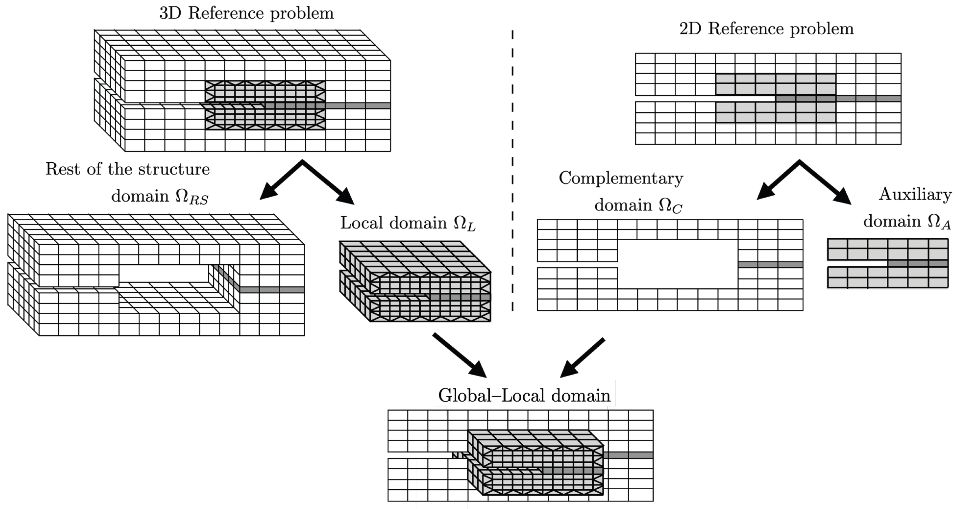
• For the 3D model: into the local domain ${\mathrm{\Omega }}_L$ that represents the area where the crack growth occurs and the rest of the structure domain ${\mathrm{\Omega }}_{RS}$, so ${\mathrm{\Omega }}_R^{3D}={\mathrm{\Omega }}_{RS}\cup {\mathrm{\Omega }}_L$.
• For the 2D model: into the auxiliary domain ${\mathrm{\Omega }}_A$ that represents the area where the crack growth occurs and the rest of the structure domain ${\mathrm{\Omega }}_C$, define as the complementary domain, so ${\mathrm{\Omega }}_R^{2D}={\mathrm{\Omega }}_A\cup {\mathrm{\Omega }}_C$.

To connect or communicate both subdomains, an interface, $\mathrm{\Gamma }$, is defined as the surface where both subdomains are in contact (${\mathrm{\Gamma }}^{3D}={\mathrm{\Omega }}_L\cap {\mathrm{\Omega }}_{RS}$ and ${\mathrm{\Gamma }}^{2D}={\mathrm{\Omega }}_A\cap {\mathrm{\Omega }}_C$), which communicates both models at the node level.

Because crack growth requires nonlinear resolution and the complete problem must be solved, the computing times are high when the complete model (2D or 3D) are large. The strategy seeks to concentrate the nonlinearities on a specific zone, which is treated nonlinearly, while the rest of the structure is solved linearly.

For the implementation of the strategy, both 2D models are of interest, while for the 3D model, only the local model is needed, as shown in Figure 1.

The first stage of resolution corresponds to solving the global linear 2D problem, Equation (7), in the complete model (${\mathrm{\Omega }}_R^{2D}$), which can be written as:

$$K_G·u_G=f_G^d$$

(7)

where $K_G$ denotes the stiffness matrix of the 2D linear global problem, $u_G$ the displacement of the nodes of the 2D structure, and $f_G^d$ the external load applied to the 2D structure.

Since only the complementary domain is needed for the strategy, Equation (7) must be modified by subtracting the response of the auxiliary domain (${\mathrm{\Omega }}_A$). This is performed by solving the linear auxiliary problem with prescribed displacements at the interface ($u_G^{\mathrm{\Gamma }}$), previously obtained by solving Equation (7). The auxiliary problem is expressed as follows.

$$\left[\begin{array}{cc}{K}_A^{\mathrm{\Gamma }\mathrm{\Gamma }}& K_A^{\mathrm{\Gamma }I}\\ K_A^{I\mathrm{\Gamma }}& K_A^{II}\end{array}\right]·\left\{\begin{array}{c}{u}_G^{\mathrm{\Gamma }}\\ u_A^I\end{array}\right\}=\left\{\begin{array}{c}{f}_A^{\mathrm{\Gamma }}\\ f_A^I\end{array}\right\}$$

(8)

where $K_A$ is the stiffness matrix of the linear auxiliary problem, ${\left\{\right\}}^{\mathrm{\Gamma }}$ represents the interface degrees of freedom, and ${\left\{\right\}}^I$ the non-interface degrees of freedom.

After solving Equation (8), the interface reactions, ${\lambda }_A$, are computed using the following expression:

$${\lambda }_A=S_A·u_G^{\mathrm{\Gamma }}+K_A^{\mathrm{\Gamma }I}·{\left[K_A^{II}\right]}^{-1}·f_A^I-f_A^{\mathrm{\Gamma }}$$

(9)

where $S_A$ correspond to the classical Schur operator obtained by

$$S_A=K_A^{\mathrm{\Gamma }\mathrm{\Gamma }}-K_A^{\mathrm{\Gamma }I}·{\left[K_A^{II}\right]}^{-1}·K_A^{I\mathrm{\Gamma }}$$

(10)

The nonlinear stage corresponds to the nonlinear local problem (3D model) with the cohesive zone method for the representation of crack growth. This stage corresponds to solving a nonlinear problem with the prescribed displacement at the interface of the model. The local displacements of the interface $u_L^{\mathrm{\Gamma }}$ are obtained by projecting the global displacements of the interface onto the 3D mesh $u_L^{\mathrm{\Gamma }}={\psi }_{GL}{u}_G^{\mathrm{\Gamma }}$, where ${\psi }_{GL}$ corresponds to a projector from the global model (2D) degrees of freedom of the interface to the local model interface degrees of freedom (3D).

The linearized tangent local problem can be written as

$$\left[\begin{array}{cc}{K}_L^{\mathrm{\Gamma }\mathrm{\Gamma }}\left(u_L\right)& K_L^{\mathrm{\Gamma }I}\left(u_L\right)\\ K_L^{I\mathrm{\Gamma }}\left(u_L\right)& K_L^{II}\left(u_L\right)\end{array}\right]·\left\{\begin{array}{c}{u}_L^{\mathrm{\Gamma }}\\ \mathrm{\Delta }{u}_L^I\end{array}\right\}=\left\{\begin{array}{c}{f}_L^{\mathrm{\Gamma }}\\ f_L^I\end{array}\right\}$$

(11)

where $K_L$ denotes the tangent stiffness matrix of the local problem. This problem can be solved by using the Newton method.

After the convergence of the Newton method, the interface reactions, ${\lambda }_L$, are obtained following a procedure similar to that for the auxiliary problem Equation (9), which can be written as

$${\lambda }_L=S_L\left(u_L\right)·({\psi }_{GL}·u_G^{\mathrm{\Gamma }})+K_L^{\mathrm{\Gamma }I}\left(u_L\right)·{\left[K_L^{II}\left(u_L\right)\right]}^{-1}·f_L^I-f_L^{\mathrm{\Gamma }}$$

(12)

where $S_L\left(u_L\right)$ corresponds to the Schur complement for the current state of the local problem.

Both auxiliary and local problems are solved with the prescribed displacement, corresponding to the primal part of the strategy.

The global–local strategy consists of subtracting the auxiliary response, ${\lambda }_A$, from the global problem, while adding the local response, ${\lambda }_L$. Finally, the strategy can be written as follows:

$$K_G·u_G-C_{\mathrm{\Gamma }G}·\left\{(K_A·u_A){\mid }_{\mathrm{\Gamma }}\right\}+C_{\mathrm{\Gamma }G}·\{{\psi }_{LG}·(K_L·u_L){\mid }_{\mathrm{\Gamma }}\}=f_G^d$$

(13)

where $C_{\mathrm{\Gamma }G}$ is the operator that relates the interface degrees of freedom to the global degrees of freedom and ${\psi }_{LG}$ (as for ${\psi }_{GL}$) corresponds to a projector from the local model interface degrees of freedom (3D) to the global model interface degrees of freedom (2D). The terms $C_{\mathrm{\Gamma }G}\left\{(K_A·u_A){\mid }_{\mathrm{\Gamma }}\right\}$ and $C_{\mathrm{\Gamma }G}\{{\psi }_{LG}·(K_L·u_L){\mid }_{\mathrm{\Gamma }}\}$ represents the response of the substructures (auxiliary or local) at the interface. Thus, Equation (13) can be rewritten as

$$K_G·u_G-C_{\mathrm{\Gamma }G}·({\lambda }_A+f_A^{\mathrm{\Gamma }})+C_{\mathrm{\Gamma }G}·{\psi }_{LG}·({\lambda }_L+f_L^{\mathrm{\Gamma }})=f_G^d$$

(14)

Rearranging the terms:

$$\begin{array}{c}\hfill K_G·u_G=f_G^d+C_{\mathrm{\Gamma }G}·(f_A^{\mathrm{\Gamma }}-{\psi }_{LG}·f_L^{\mathrm{\Gamma }})+C_{\mathrm{\Gamma }G}·({\lambda }_A-{\psi }_{LG}·{\lambda }_L)\end{array}$$

(15)

since the expression $C_{\mathrm{\Gamma }G}·(f_A^{\mathrm{\Gamma }}-{\psi }_{LG}·f_L^{\mathrm{\Gamma }})$ cancels to zero because $f_A^{\mathrm{\Gamma }}$ and ${\psi }_{LG}·f_L^{\mathrm{\Gamma }}$ both correspond to the same external load applied to the interface. Finally, the global problem can be written as

$$\begin{array}{c}\hfill K_G·u_G=f_G^d+C_{\mathrm{\Gamma }G}·({\lambda }_A-{\psi }_{LG}·{\lambda }_L)\end{array}$$

(16)

The expression $C_{\mathrm{\Gamma }G}·({\lambda }_A-{\psi }_{LG}·{\lambda }_L)$ corresponds to the interface load correction applied to the global model, to include the effect of the development of nonlinearity in the local model. This interface load correction for the global problem corresponds to the dual part of the strategy.

A residual is computed between two iterations by performing the following:

$$r^n=C_{\mathrm{\Gamma }G}·\{({\lambda }_A^n-{\psi }_{LG}·{\lambda }_L^n)-({\lambda }_A^{n-1}-{\psi }_{LG}·{\lambda }_L^{n-1})\}$$

(17)

where super-index ⁿ corresponds to the current iteration n.

To evaluate the convergence of the strategy, the norm of the current residual is compared with the norm of the first residual:

$$\eta ={\displaystyle \frac{\left|\right|r^n{\left|\right|}_2}{\left|\right|r^1{\left|\right|}_2}}$$

(18)

2.3. Global–Local Algorithm

The Algorithm 1 presents the stages of the implemented global–local method.

Algorithm 1 Primal–Dual Global–Local strategy

while $\eta >{\eta }^{crit}$ do     Solve linear global problem     $K_G·u_g^n=f_G^d+C_{\mathrm{\Gamma }G}·({\lambda }_A^{(n-1)}-{\psi }_{LG}·{\lambda }_L^{(n-1)})$                      ▹${\lambda }_A$ and ${\lambda }_L$ are 0 for the first iteration     Solve linear auxiliary problem     $K_A·u_A^n=f_A^d$          ▹ with prescribed displacements, ${u_A^{\mathrm{\Gamma }}}^n={u_G^{\mathrm{\Gamma }}}^n$     Compute ${\lambda }_A$     Solve nonlinear local problem (Newton Raphson)     $K_L\left(u_L^n\right)·u_L^n=f_L^d$      ▹ with prescribed displacements, ${u_L^{\mathrm{\Gamma }}}^n={\psi }_{GL}·{u_G^{\mathrm{\Gamma }}}^n$     Compute ${\lambda }_L$     Compute residual     $r^n=C_{\mathrm{\Gamma }G}·\{({\lambda }_A^n-{\psi }_{LG}·{\lambda }_L^n)-({\lambda }_A^{n-1}-{\psi }_{LG}·{\lambda }_L^{n-1})\}$     Compute error criteria     $\eta ={\displaystyle \frac{\left|\right|r^n{\left|\right|}_2}{\left|\right|r^1{\left|\right|}_2}}$ end while

3. Results of Global–Local Analysis

In this section, the global–local methodology is evaluated in a DCB test, with the objective of validating the methodology for this complex test and defining some criteria for selecting the size of the local problem.

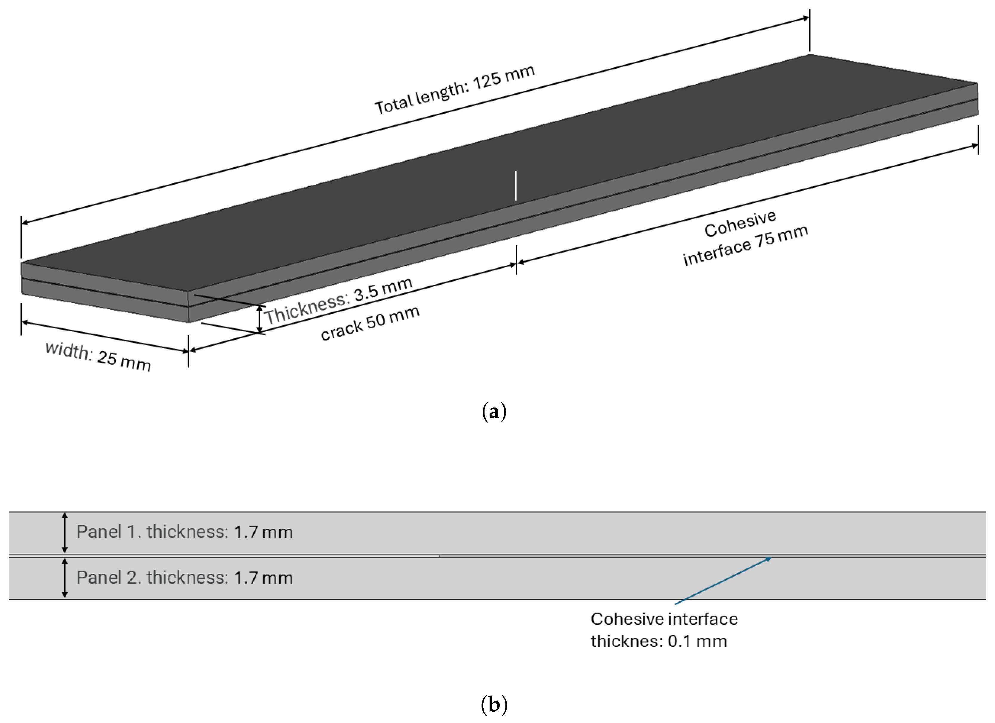
3.1. DCB Test

The specimen model comprised two laminates, each measuring 125 mm in length, 25 mm in width, and 1.7 mm in thickness. These laminates exhibited identical mechanical properties and were bonded along a cohesive zone measuring 75 mm in length, 25 mm in width, and 0.1 mm in thickness (see Figure 2). A vertical displacement of 10 mm was imposed at the end of the two loading points located at the ends of the specimen arms, simultaneously and symmetrically with respect to the midplane of the specimen. These displacements were applied in 10 steps for the monolothic model (without decomposition) and in 1 step for the decomposed model (global-local model).

The geometric details of the model are shown in Figure 2. The propagation of the crack occurred within the cohesive zone, progressively separating the plates as the externally applied loads increased. This continued until the cohesive forces of the adhesive material equilibrated with the bending moment generated by the external loads and the distance to the crack tip.

The analysis assumes an isotropic material for laminates, with the mechanical properties defined as Young’s modulus $E_1$ = 157 GPa, Poisson’s ratio ${\nu }_1$ = 0.3.

For the cohesive zone parameters, the values used were obtained from an example of their implementation presented in the documentation of the Code Aster software. Finally, the values used are as follows: Young’s modulus, $E_1$ = 100 MPa; Poisson’s ratio, ${\nu }_1$ = 0; critical energy density, $G_c$ = 0.2 mJ/mm²; and other parameters such as pena-adherence, $P_{adh}$ = 0.00001 N/m, which corresponds to the adhesion penalty, that is, the sliding capacity of surfaces whose value varies between 0 and 1. Small values allow some sliding, while large values impose more rigid restrictions; pena-lagr, $P_{lag}=100.000$ N/m, is a numerical penalty stiffness that controls the tangential (sliding) behavior of the cohesive interface. It acts to penalize relative tangential displacements between cohesive surfaces in contact, helping to prevent numerical instabilities; while not a Lagrangian multiplier in the classical sense, this parameter introduces a tangential stiffness that stabilizes the interface response under frictionless or low-friction conditions, particularly when cohesive elements are used to model delamination or interfacial damage; rigi-glis $k_t$ = 100 defines the tangential stiffness of the contact (or of the adhesion and slip model); ${\sigma }_c$ = 3 MPa.

The cohesive zone is modeled with Poisson’s ratio $\nu =0$, effectively enforcing a decoupled, uniaxial opening response consistent with pure mode I. This choice ensures the traction–separation law operates solely on normal opening displacements, improving numerical stability. For more realistic materials, a Poisson’s ratio between $\nu =0.3$ and $\nu =0.4$ is commonly used, as presented in the state of the art [37,38].

3.2. Studied Cases

To evaluate the influence of the size of the local nonlinear problem, three cases were analyzed:

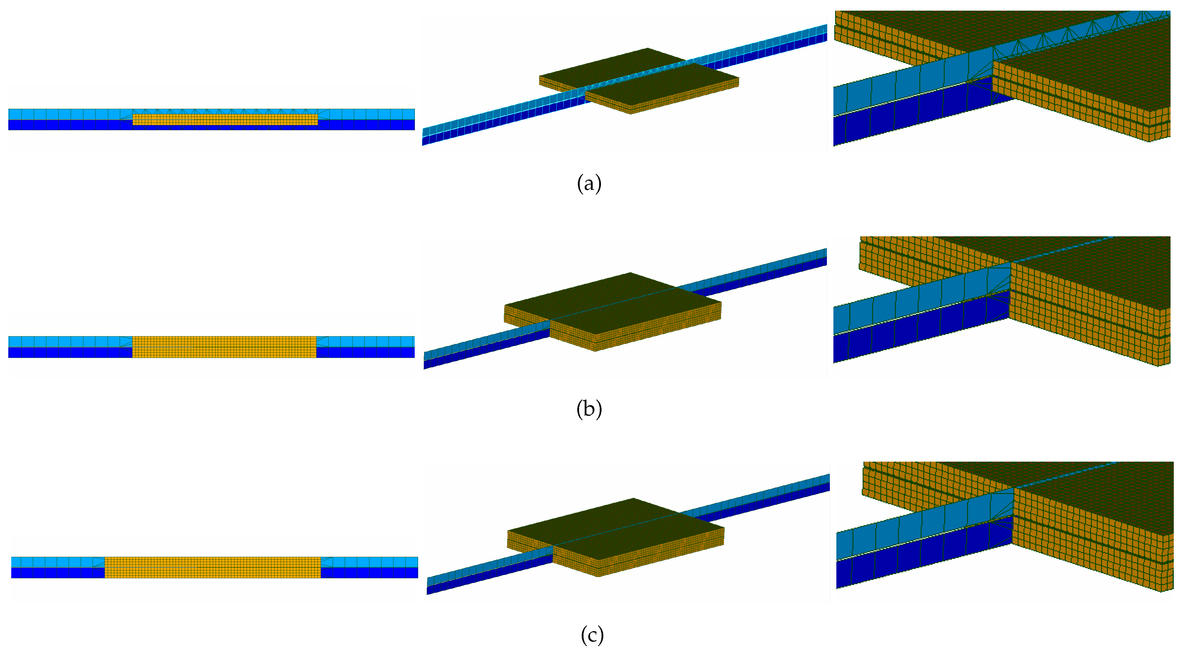
• Case I: the local problem covers 50% of the total thickness of the plate with a length of 30 mm, including 10 mm of pre-crack, Figure 3a.
• Case II: the local problem covers the entire thickness of the test, with the same length of 30 mm, including 10 mm of pre-crack, Figure 3b.
• Case III: the local problem covers the entire thickness of the test, with a length of 35 mm, including 15 mm of pre-crack, Figure 3c.

For all the cases, three different meshes are used for the local problems, defined by the size of the element, 1 mm, 0.625 mm and 0.5 mm, giving 2, 3 and 4 elements on the thickness of each plate. For global problems, the same size of 2 mm is used for the elements, which gives one element on the thickness of each plate. In order to connect both models, the global one has a refinement on the nodes in contact with the local model in order to obtain compatible meshes.

The number of nodes for each model is presented in

Table 1. Number of nodes for every model.

Case/Model (Mesh Size)		Number of Nodes
		1 mm	0.625 mm	0.5 mm
Monolithic		19,656	65,928	128,010
Case I	Global	288	288	288
	Local	3224	12,054	18,666
Case II	Global	256	256	256
	Local	4836	16,072	31,110
Case III	Global	256	256	256
	Local	5616	18,696	36,210

. For all three analyzed cases, the global problem has very few nodes, the local model has a larger number of nodes, and the reference model, the monolithic model, has an even larger number of nodes.

Additionally, the mesh quality was evaluated using the aspect ratio parameter.

Table 2. Aspect ratios for every model.

Aspect Ratio	Monolithic Models	Global Models	Local Models
<1.5	-	panels	-
1.5–>5	panels	-	panels
5–>10	-	-	-
>10	cohesive zone	cohesive zone	cohesive zone

presents the corresponding values for each region of the meshes. For all monolithic models, an average aspect ratio of approximately 3.5 was observed in the plates, while values exceeding 10 were found in the cohesive zone. This pattern is consistent across all local models. In contrast, the global models exhibit improved mesh quality in the plates, with aspect ratios below 1.5; however, poor mesh quality persists in the cohesive zone.

Although the mesh quality in the cohesive zone shows high aspect ratio values, the focus of the present study was on assessing the influence of the local model size rather than optimizing element quality.

The solutions of the global/local models are compared with the reference problem using: deformation, nodal forces, stress distribution, displacement of the crack tip, and computation times.

As a reference solution, the complete problem is solved using a 3D mesh and a cohesive zone model, employing the same mesh size as the corresponding local model. For each of the three local mesh sizes considered, a reference model is generated, referred to as ’monolithic’, since the solution involves a single global model of the structure without any decomposition.

3.3. Results

3.3.1. Convergence of the Different Cases

In all the cases studied, the method converges to very small values after four iterations (see Figure 4). For case I and case II with a mesh size of 1 mm and case III with a mesh size of 0.5 mm, the error goes directly to 0, while for the other cases, the error tends to ${10}^{-15}$ or lower, showing that the methodology has converged.

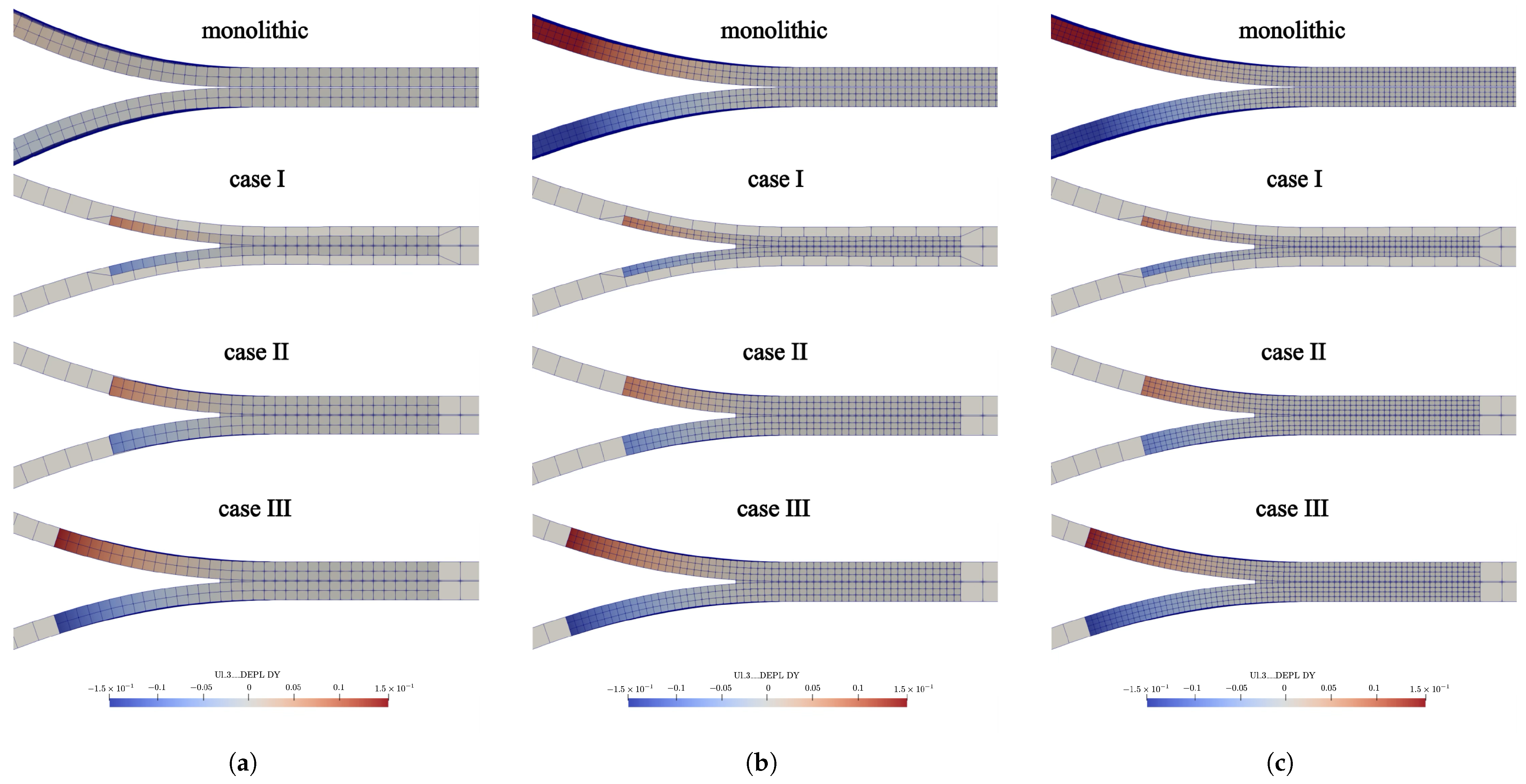
3.3.2. Deformation

In Figure 5, the displacement responses of the different cases analyzed are shown. For all cases and for the different mesh sizes, the results show that the models are well connected, representing the response of the structure to the loads. The global models followed the expected deformations, while the local models were well attached to them.

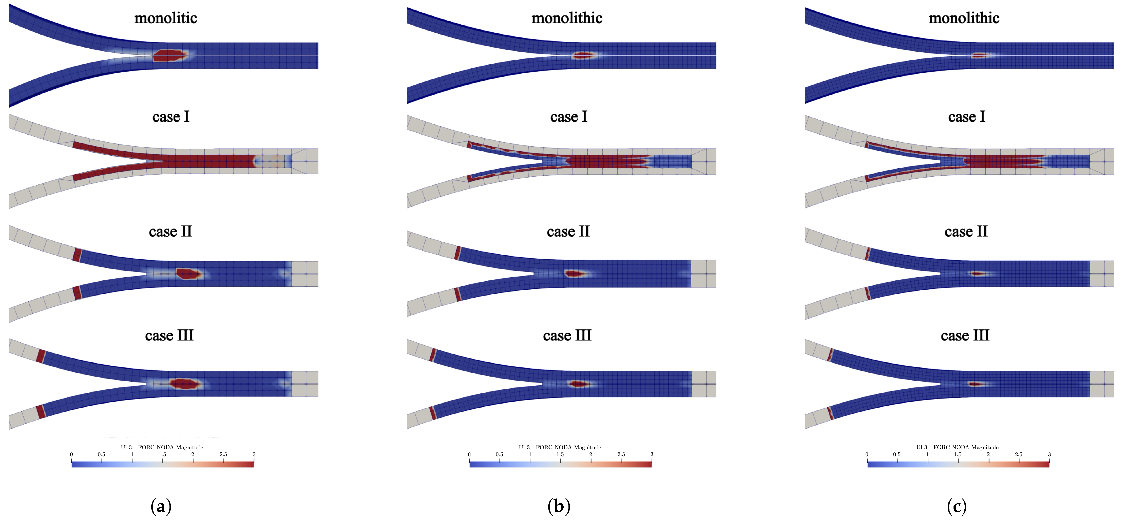
3.3.3. Nodal Forces

In Figure 6, the vertical nodal forces are presented for all cases. The vertical nodal forces are responsible for opening the crack. For cases I, II, and III, only the nodal forces on the local model are shown.

As expected, these loads should be greater around the crack tip, which can be appreciated on the monolithic case, case II, and case III. However, for case I, because the connecting interface is horizontal, the transmitted load/displacement between the global and local models is vertical to enforce the continuity of the models. Finally, the vertical nodal forces are distorted over the complete local model due to its thickness. The influence of this behavior is somehow reduced when the mesh is refined.

Cases II and III accurately represent the distribution of the vertical nodal forces of the monolithic model, depending only on the mesh size.

3.3.4. Stress Distribution

In Figure 7, the von Mises stress distributions are presented for all the cases analyzed. For cases I, II, and III, only the stresses on the local models are shown. Similarly to the vertical nodal forces (see Section 3.3.3), the stress distribution for case I is affected by the interface compensation loads, which are a few elements away from any part of the local model. This can be explained by Saint-Venant’s principle, which states that the stress distribution is affected near the load application points, such as the stress concentration. Because the zone of interest, that is, the tip of the crack, is quite close to the interface in terms of the number of elements, the stresses are highly distorted in this area.

For cases II and III, the stress distribution was accurate with respect to the monolithic response and improved with the refinement of the local model.

3.3.5. Crack Tip Displacement

In

Table 3. Comparative crack tip displacement between analysis methods with different element size meshes.

Monolithic Model [mm]	Case	Element Size [mm]	Global/Local Model [mm]	Error
4.4573	Case I	1	4.9767	11.65%
		0.625	4.3437	2.55%
		0.5	4.4717	0.32%
	Case II	1	4.9899	11.95%
		0.625	4.3576	2.23%
		0.5	4.4852	0.62%
	Case III	1	4.9926	12.01%
		0.625	4.3247	2.97%
		0.5	4.4858	0.64%

, the displacement of the tip crack is presented for all cases analyzed. A monolithic solution with the most refined mesh was used as a reference.

The results for the different cases are similar for each element size.

For the same element size, case III has a slightly higher error than case I and case II. This may be attributed to the projection process between the global and local models, where increasing the size of the local domain, a larger local model domain encompassing a broader portion of the structure, may induce a different distribution of internal loads on the local model. However, the difference in accuracy is relatively small, suggesting that both configurations yield consistent results within an acceptable error range.

An oscillatory convergence behavior with mesh refinement can be observed. Although non-monotonic behavior is observed, the amplitude of the variations decreases with refinement, suggesting a trend towards asymptotic convergence. This behavior can be attributed to the following factors:

• Interpolation effects between meshes of different refinement levels, which leads to local over- or underestimation of displacement, particularly when displacement fields exhibit steep gradients or discontinuities associated with crack propagation.
• Mesh quality in the cohesive zone, particularly the aspect ratio and distortion of the elements aligned with the crack path, may significantly affect the accuracy and stability of the results. Poor mesh quality in this region can lead to artificial stiffness or premature damage localization, which in turn influences the calculated displacements and contributes to the oscillatory convergence behavior observed in the results.
• Discrete positioning of the crack front, as mesh refinement improves the accuracy of the crack front representation. This may cause the crack to interact differently with the structure and boundary conditions, resulting in slight variations in the magnitude of the maximum displacement.

It can be concluded that the error in the tip crack displacement does not depend on the size of the local problem or the position of the interfaces, even if they are close to the zone of interest, but depends only on the size of the elements. Finally, for all cases, it can be said that the larger the mesh, the larger the error.

3.3.6. Computation Time

One of the main objectives of this type of methodology corresponds to a reduction in the size of the problem, as shown in Table 1, as well as a reduction in the computation time. For this study, even with a small and simple structure, such as the DCB test, some time savings were achieved. In

Table 4. Comparative time between analysis methods with different element size meshes.

Monolithic Model [s]	Case	Element Size [mm]	Global/Local Model [s]	Time Saving
2297.64	Case I	1	118	94.9%
		0.625	523	77.2%
		0.5	968	57.9%
	Case II	1	171	92.6%
		0.625	740	67.8%
		0.5	1671	27.3%
	Case III	1	183	92.0%
		0.625	947	58.8%
		0.5	2105	8.4%

, the computation times are listed for all the cases analyzed, and the % savings are presented. As a reference, the computation time for the monolithic model with the most refined mesh is used.

Even if the strategy is applied on a global/local problem which is smaller in terms of total nodes, the different stages of the methodology require multiple communication between the models, increasing the computation time. Nevertheless, in this case, the size of the local problem is on the same order of magnitude as the monolithic model, whereas for a real case with larger structures, the local problem could be a few orders of magnitude smaller than the monolithic model, implying a larger reduction in computing time.

4. Conclusions

This work presented and validated a non-intrusive primal–dual global–local strategy for simulating crack propagation in a DCB test using cohesive zone models. The approach successfully reproduced the mechanical response of a full 3D monolithic model while substantially reducing computational cost through domain decomposition. The results demonstrate that the proposed methodology yields highly accurate displacement, force, and stress fields, particularly when the local model fully represents the structural thickness and is appropriately meshed.

The convergence behavior was consistent across all test cases, confirming the robustness of the algorithm regardless of the size and resolution of the local model. Notably, the crack tip displacement errors decreased to less than 1% in the most refined cases, and computational time savings reached up to 90%, even in this relatively small-scale problem.

From a scientific standpoint, the study confirms that mesh resolution is the dominant factor affecting numerical accuracy, rather than the position or size of the local model domain. Furthermore, the stress distortion observed in limited local configurations highlights the importance of choosing local domains that adequately capture the structural thickness and fracture process zone.

The studied methodology offers a scalable and efficient framework for simulating fracture in large structures. Its flexibility makes it suitable for more complex configurations involving anisotropic materials, rolling shear phenomena, or large-scale CLT panels. This work contributes to advancing non-intrusive multiscale strategies in fracture mechanics and paves the way for future research involving structural-scale simulations of delamination in laminated timber structures.

References

- Blanco, C.; Cabrero, J.; Martin-Meizoso, A.; Gebremedhin, K. Design oriented failure model for wood accounting for different tensile and compressive behavior. Mech. Mater. 2015, 83, 103–109. [Google Scholar] [CrossRef]
- Mackenzie-Helnwein, P.; Eberhardsteiner, J.; Mang, H.A. A multi-surface plasticity model for clear wood and its application to the finite element analysis of structural details. Comput. Mech. 2003, 31, 204–218. [Google Scholar] [CrossRef]
- Sedighi-Gilani, M.; Navi, P. Micromechanical approach to wood fracture by three-dimensional mixed lattice-continuum model at fiber level. Wood Sci. Technol. 2007, 41, 619–634. [Google Scholar] [CrossRef]
- de Moura, M.; Dourado, N.; Morais, J. Crack equivalent based method applied to wood fracture characterization using the single edge notched-three point bending test. Eng. Fract. Mech. 2010, 77, 510–520. [Google Scholar] [CrossRef]
- Saavedra, E.I.; Saavedra, K.; Hinojosa, J.; Chandra, Y.; Das, R. Multi-scale modelling of rolling shear failure in cross-laminated timber structures by homogenisation and cohesive zone models. Int. J. Solids Struct. 2016, 81, 219–232. [Google Scholar]
- Dourado, N.; de Moura, M.; Morais, J.; Silva, M. Estimate of resistance curve in wood through the double cantilever beam test. Holzforschung 2010, 64, 119–126. [Google Scholar] [CrossRef]
- Dourado, N.; Morel, S.; de Moura, M.; Valentin, G.; Morais, J. Comparison of fracture properties of two wood species through cohesive crack simulations. Compos. Part A Appl. Sci. Manuf. 2008, 39, 415–427. [Google Scholar] [CrossRef]
- Hashin, Z. Finite thermoelastic fracture criterion with application to laminate cracking analysis. J. Mech. Phys. Solids 1996, 44, 1129–1145. [Google Scholar] [CrossRef]
- Nairn, J.A. Predicting layer cracks in cross-laminated timber with evaluations of strategies for suppressing them. Eur. J. Wood Wood Prod. 2019, 77, 1–15. [Google Scholar] [CrossRef]
- Moës, N.; Dolbow, J.; Belytschko, T. A finite element method for crack growth without remeshing. Int. J. Numer. Methods Eng. 1999, 46, 131–150. [Google Scholar] [CrossRef]
- Belytschko, T.; Black, T. Elastic crack growth in finite elements with minimal remeshing. Int. J. Numer. Methods Eng. 1999, 45, 601–620. [Google Scholar] [CrossRef]
- Zhou, Q.; Gong, M.; Chui, Y.H.; Mohammad, M. Measurement of rolling shear modulus and strength of cross laminated timber fabricated with black spruce. Constr. Build. Mater. 2014, 64, 379–386. [Google Scholar] [CrossRef]
- Christovasilis, I.P.; Brunetti, M.; Follesa, M.; Nocetti, M.; Vassallo, D. Evaluation of the mechanical properties of cross laminated timber with elementary beam theories. Constr. Build. Mater. 2016, 122, 202–213. [Google Scholar] [CrossRef]
- Perret, O.; Lebee, A.; Douthe, C.; Sab, K. The Bending–Gradient theory for the linear buckling of thick plates: Application to Cross Laminated Timber panels. Int. J. Solids Struct. 2016, 87, 139–152. [Google Scholar] [CrossRef]
- Pina, J.C.; Saavedra, E.; Saavedra, K. Numerical study on the elastic buckling of cross-laminated timber walls subject to compression. Constr. Build. Mater. 2019, 199, 82–91. [Google Scholar] [CrossRef]
- Park, K.; Paulino, G.H. Cohesive zone models: A critical review of traction-separation relationships across fracture surfaces. Appl. Mech. Rev. 2011, 64, 060802. [Google Scholar] [CrossRef]
- Turon, A.; Bak, B.L.V.; Lindgaard, E.; Sarrado, C.; Lund, E. Interface elements for delamination in composite laminates: Constitutive modeling. Mech. Adv. Mater. Struct. 2018, 25, 915–923. [Google Scholar]
- Qingfeng, D.; Haixiao, H.; Dongfeng, C.; Wei, C.; Shuxin, L. A new mechanism based cohesive zone model for Mode I delamination coupled with fiber bridging of composite laminates. Compos. Struct. 2024, 332, 117931. [Google Scholar]
- Wu, J.-Y.; Nguyen, V.P.; Nguyen, C.T.; Sutula, D.; Bordas, S.; Sinaie, S. Phase field modeling of fracture. Adv. Appl. Mech. 2017, 53, 1–183. [Google Scholar]
- Dolbow, J.; Sargado, J.M.; Jiang, T.; Borden, M.J. A phase-field description of dynamic cohesive fracture. Comput. Methods Appl. Mech. Eng. 2021, 387, 114118. [Google Scholar]
- Zhou, F.; Molinari, J.-F. Dynamic crack propagation with cohesive elements: A methodology to address mesh dependency. Int. J. Numer. Methods Eng. 2004, 59, 1–24. [Google Scholar] [CrossRef]
- Spring, D.W.; Leon, S.E.; Paulino, G.H. Unstructured polygonal meshes with adaptive refinement for the numerical simulation of dynamic cohesive fracture. Int. J. Fract. 2016, 189, 33–57. [Google Scholar] [CrossRef]
- Valoroso, N.; Champaney, L.; Boucard, P.-A.; Guinard, S. Identification of cohesive zone parameters using an inverse method coupled to a genetic algorithm. Int. J. Fract. 2013, 179, 129–147. [Google Scholar]
- Chen, C.T.; Gu, G.X.; Zhu, J.; Sun, W.; Fang, N.X.; Rider, W.J. Data-driven multi-scale multi-physics models to predict the effects of crack morphology on ceramic fracture. J. Mech. Phys. Solids 2020, 143, 104048. [Google Scholar]
- Reinoso, J.; Paggi, M. A consistent interface element formulation for geometrical and material nonlinearities. Comput. Mech. 2014, 54, 1569–1581. [Google Scholar] [CrossRef]
- Guidault, P.-A.; Allix, O.; Champaney, L.; Cornuault, C. A multiscale extended finite element method for crack propagation. Comput. Methods Appl. Mech. Eng. 2008, 197, 381–399. [Google Scholar] [CrossRef]
- Kerfriden, P.; Allix, O.; Gosselet, P. A three-scale domain decomposition method for the 3D analysis of debonding in laminates. Comput. Mech. 2009, 44, 343–362. [Google Scholar] [CrossRef]
- Loehnert, S.; Belytschko, T. A multiscale projection method for macro/microcrack simulations. Int. J. Numer. Methods Eng. 2007, 71, 1466–1482. [Google Scholar] [CrossRef]
- Wohlmuth, B.; Farah, P.; Hirschberger, C.B.; Borst, R.; Wriggers, P. A computational framework for interface failure analysis accounting for plasticity, damage and frictional effects. Comput. Mech. 2022, 69, 1371–1392. [Google Scholar]
- Ibrahim, A.H.; Watson, B.; Jahed, H.; Rezaee, S.; Cronin, D.S. An experimental-cohesive zone model approach to predict fatigue life of adhesive joints with varying modes of loading and joint configurations for automotive applications. J. Adhes. 2024, 69, 1–27. [Google Scholar] [CrossRef]
- Özdemir, İ.; Brekelmans, W.A.M.; Geers, M.G.D. A thermo-mechanical cohesive zone model. Comput. Mech. 2010, 46, 735–745. [Google Scholar] [CrossRef]
- Whitcomb, J.D. Iterative global/local finite element analysis. Comput. Struct. 1991, 40, 1027–1031. [Google Scholar] [CrossRef]
- Gendre, L.; Allix, O.; Gosselet, P.; Comte, F. Non-intrusive and exact global/local techniques for structural problems with local plasticity. Comput. Mech. 2009, 44, 233–245. [Google Scholar] [CrossRef]
- Fuenzalida-Henríquez, I.; Oumaziz, P.; Castillo-Ibarra, E.; Hinojosa, J. Global-Local non intrusive analysis with robin parameters: Application to plastic hardening behavior and crack propagation in 2D and 3D structures. Comput. Mech. 2022, 69, 965–978. [Google Scholar] [CrossRef]
- Jaque-Zurita, M.; Hinojosa, J.; Castillo-Ibarra, E.; Fuenzalida-Henríquez, I. Discriminant analysis based on the patch length and crack depth to determine the convergence of Global-Local Non-intrusive analysis with 1D-to-3D coupling. Symmetry 2023, 15, 2068. [Google Scholar] [CrossRef]
- Jaque-Zurita, M.; Hinojosa, J.; Fuenzalida-Henríquez, I. Global-Local non intrusive analysis with 1D to 3D coupling: Application to crack propagation and extension to commercial software. Mathematics 2023, 11, 2540. [Google Scholar] [CrossRef]
- Blackman, B.R.K.; Hadavinia, H.; Kinloch, A.J.; Williams, J.G. The use of a cohesive zone model to study the fracture of fibre composites and adhesively-bonded joints. Int. J. Fract. 2003, 119, 25–46. [Google Scholar] [CrossRef]
- Carvalho, U.T.F.; Campilho, R.D.S.G. Validation of a direct method to predict the strength of adhesively bonded joints. Sci. Technol. Mater. 2018, 30, 138–143. [Google Scholar] [CrossRef]