Evaluating the Effectiveness of Natural Carbon Sinks Through a Temperature-Dependent Model

Abstract

Articles have recently been circulating in the media around the world, claiming that natural ${\mathrm{CO}}_2$ sinks have “suddenly and unexpectedly” ceased to function. It turned out that these articles were based on a single preprint of a meanwhile published article. Its reasoning is essentially based on the large spike of ${\mathrm{CO}}_2$ concentration growth in 2023 despite constant anthropogenic emissions. However, there are no obvious indications that photosynthesis or oceanic sinks have decreased. In this paper, it is shown that besides the natural sink systems of the land plants and oceans, the variability of natural emissions has to be considered. Based on a previous publication, it is made evident that natural emissions are temperature-dependent. Therefore, the careful analysis of monthly sea surface temperature and ${\mathrm{CO}}_2$-concentration data for 2023 and 2024 gives a consistent explanation for the rise in atmospheric carbon concentration growth without referring to the implausible hypothesis of failing carbon sinks. The temperature dependence of natural ${\mathrm{CO}}_2$ emissions indicates a clear causality from temperature to ${\mathrm{CO}}_2$ concentration. This is confirmed by the time shift between temperature and the subsequent concentration change. This suggests a new component in climate models with implications for climate policies.

1. Introduction

Articles are currently being circulated in the media claiming that natural ${\mathrm{CO}}_2$ sinks have “suddenly and unexpectedly” ceased to function. The natural ${\mathrm{CO}}_2$ reservoirs are the biota, consisting of all living organisms, plants, animals and humans. In addition, the oceans store around 50 times the amount of atmospheric ${\mathrm{CO}}_2$. It is known and has been proven for many decades that both the biota and the oceans are strong ${\mathrm{CO}}_2$ sinks. Currently, more than half of all anthropogenic emissions are absorbed by the two major sink systems, ocean and land plants, as reported in [1].

What has happened that suddenly the sink effect is supposedly diminishing? Even at first glance, the diagram (Figure 3) in [1] reveals that the sink effect, which is attributed to land plants, is subject to extraordinarily strong fluctuations, much more so than in the case of the oceans, for example. This should immediately make us suspicious when we talk about a “one-off” event within the past year.

The scientific basis and trigger for the current discussion is the recent article: “Low latency carbon budget analysis reveals a large decline of the land carbon sink in 2023” [2]. The publication essentially states that anthropogenic emissions have been more or less constant over the recent years, but atmospheric ${\mathrm{CO}}_2$ concentration grew much more than usual in 2023, while between 2016 and 2022 concentration growth was steadily declining. Their conclusion from this observation is that the systems responsible for ${\mathrm{CO}}_2$ absorption, such as land plants or cold oceans, must have been failing. Another publication from the Alfred Wegener Institute (AWI) in Germany investigated the ocean uptake of ${\mathrm{CO}}_2$ since 1958 [3]. They came to the conclusion that the ocean sink is diminishing; besides wind, they identified increasing temperature as a sink-diminishing factor.

Other investigations have found convincing evidence that land sinks have, in fact, significantly increased due to ${\mathrm{CO}}_2$ fertilization, particularly in tropical forest regions and reduced cold-limitations due to elevated temperature, primarily at higher latitudes [4]. Moreover, this overview article gives good reasons for the future increase of land sinks. In particular, the CMIP6 climate models predict increasing land sinks for at least the next 30 years in the RCP2.6 and higher scenarios [5]. In a recent publication, it was discovered by means of a new analysis that, in fact, the gross primary production (GPP) is 25% larger than previously assumed [6], and in particular, the GPP is 5% larger than soil respiration.

Such evidence suggests that there may be a forgotten factor in the understanding of the carbon cycle. We may have to look for another explanation causing changes in ${\mathrm{CO}}_2$ concentration growth. Evaluating the literature on carbon sinks gives some hints on where to look for an answer for the apparent deviations. Roy Spencer introduced El Ni$\tilde{n}$o as a possible cause to balance the apparently declining carbon sink activity [7]. Ferdinand Engelbeen used a similar argument to explain short-term atmospheric ${\mathrm{CO}}_2$ concentration changes depending on temperature anomalies [8], but from that publication, it is not clear exactly what he means by temperature anomaly. In an earlier publication on his blog [9], he indicates (in the legend of the first graph) that his understanding of temperature anomaly is the time derivative of temperature, contrary to the standard definition of temperature anomaly, defined it as the temperature difference to a fixed earlier baseline temperature.

Outline of the Article

A previous paper [10] introduced the global sea surface temperature irrespective of the ${\mathrm{CO}}_2$ concentration as an additional predictor of the carbon sink effect, resolving the contradiction between the apparent temperature trend independence of the sink effect and the obvious temperature trend of global temperature anomalies as a consequence of the high correlation between the global temperature anomaly and ${\mathrm{CO}}_2$ concentration.

The described model could only make statements about the difference between absorptions and natural emissions because only their difference can be easily measured from available global data. It could not tell whether a specific reduction in the measured sink effect was due to a reduction in absorption or an increase in natural emissions.

Previous publications were restricted by yearly data. The fast change in ${\mathrm{CO}}_2$ concentration growth over 2023 and 2024 motivates a higher resolution. In particular, the potential time lag between temperature change and change in the sink effect will have to be investigated—it is expected to be several months.

This article includes additional evidence from two more sources. The decay of the atmospheric ¹⁴C concentration after the nuclear test ban treaty 1963 gives an indication of the absorption rate. This will help to separate the downwelling carbon flow from the upwelling emissions.

The other source of additional evidence is studies investigating the temperature dependence of natural emissions by the two main emitters, the biological decay and the outgassing from oceans.

This article brings together different sources of evidence in order to develop a consistent model of the atmospheric carbon cycle. This will help to clarify the recent anomalies of the atmospheric concentration growth of ${\mathrm{CO}}_2$.

2. Materials and Methods

The approach taken here is not to investigate possible individual sources or sinks and their specific mechanism, that would be the bottom-up approach. Instead, a top-down approach is taken. The sources of information are global measurable data, notably ${\mathrm{CO}}_2$ concentration measured at Mauna Loa [11], the global anthropogenic emissions, as defined in the Global Carbon Budget [1], and the global average sea surface temperature [12].

For validation purposes, other sources of information are included. One of them, the ¹⁴C concentration data after the bomb test treaty in 1963, is also a global data set [13].

All types of emissions, except explicit anthropogenic emissions, are considered here to be part of the unknown natural emissions, in particular, the land use change emissions. This decision has been discussed in [10]. The variability of these natural emissions is constrained by the residual of the introduced models.

In the publications “Emissions and CO₂ Concentration—An Evidence Based Approach” [14] and “Improvements and Extension of the Linear Carbon Sink Model” [10], the relationship among yearly data of emissions, concentration increase, and sink effect was analyzed and a robust, simple model of the sink effect was developed that not only reproduces the measurement data of the last 70 years very accurately but also allows reliable forecasts. For example, the concentration data for the years 2000–2020 were predicted with extremely high accuracy from the emissions and the model parameters determined before the year 2000. However, the most recent series of measurements used in the publications ended in December 2022 and annual averages were used, so the phenomena that are currently causing so much excitement were not yet taken into account.

This article builds on the evidence gained by these previous papers and develops the models further by introducing monthly data resolution and considering time shifts between temperature change and its effect.

2.1. The Top-Down Carbon Sink Model from the Continuity Equation

The continuity equation based on the conservation of mass implies that the atmospheric concentration growth $G_i$ in year i results from the difference between the total emissions and all absorptions $A_i$ [14], whereby the total emissions are the sum of the anthropogenic emissions $E_i$ and the natural emissions $N_i$, i.e.,

$$G_i=E_i+N_i-A_i$$

(1)

The effective sink capacity $S_i$ is calculated as the difference between the anthropogenic emissions $E_i$ and the concentration growth $G_i$, i.e.,

$$S_i=E_i-G_i$$

(2)

Following the continuity equation above, the effective sink capacity $S_i$, therefore, is the difference of ocean and plant absorptions $A_i$ and natural emissions $N_i$:

$$S_i=A_i-N_i$$

(3)

It is important to note that the sink effect consists of two components, the actual absorptions and the natural emissions. When measuring the sink effect, we do not know anything about the actual absorptions $A_i$ nor about the natural emissions $N_i$. All models for the sink effect $S_i$ have this conceptual deficit. Nevertheless, they are the starting point of this investigation.

A simple linear sink model for Equation (3) has been developed by several researchers [7,14,15,16,17,18], where the sink effect of the yearly data model only depended on the ${\mathrm{CO}}_2$ concentration of the previous year $C_{i-1}$ with an offset $C^0$, representing an equilibrium concentration:

$$\begin{array}{ccc}\hfill {\widehat{S}}_i\left(C\right)& =& a^{\prime }·(C_{i-1}-C^0)\hfill \end{array}$$

(4)

$$\begin{array}{ccc}& =& a^{\prime }·C_{i-1}-n\hfill \end{array}$$

(5)

The parameters $a^{\prime }$ and n are determined by minimizing the sums of squares between measured data from Equation (2) and the sink model of Equation (5) over all known years i:

$$\underset{a^{\prime },n}{min}\sum _i{\left(E_i-G_i-(a^{\prime }·C_{i-1}-n)\right)}^2$$

(6)

All statistical evaluations, in particular, the ordinary least squares optimization, were conducted with the Python package Statmodels, version 0.13.5 [19], and the graphs were created with the Python package Matplotlib, version 3.7.0 [20].

$n=a^{\prime }·C^0$ represents the assumed constant natural net emissions per year. Obviously, this is a very crude model because with the constant n it is not possible to represent any systematic variability.

Questions about the principle validity of this model for multiple sinks have made it necessary to again clarify a point that has been discussed before [14,16]. The total sink effect is composed of the sum of several linearized components, which may have different equilibrium concentrations. Let us pick ocean, phytoplankton, ${\mathrm{C}}_3$ plants, and ${\mathrm{C}}_4$ plants [21]:

$${\widehat{S}}_i\left(C\right)=a_{ocean}·(C_i-C_{ocean}^0)+a_{phyto}·(C_i-C_{phyto}^0)+a_{C3}·(C_i-C_{C3}^0)+a_{C4}·(C_i-C_{C4}^0)$$

(7)

As this is a linear form, it maps perfectly into the form of Equation (5). The individual sink rates or their equilibrium value remain unknown, only their combined effect is determined.

Land use change effects are not considered here as anthropogenic. They are assumed to be part of the unknown natural emissions. In a previous publication, land use change emissions have been included as part of the anthropogenic emissions [14], pulling down the resulting equilibrium concentration to 242 ppm. This contradicts the accepted consensus that the pre-industrial equilibrium concentration was between 270 ppm and 290 ppm. Furthermore, [10] demonstrated that prediction quality improves when land use change emissions are discarded as explicit anthropogenic emissions during the time since 1959. Land use change emissions might have had a significant role in the first half of the 20th century [10], this will be subject to future research.

2.1.1. Finding the Appropriate Data Resolution

There are two aspects that motivate the observation of monthly data. Primarily, the rise in concentration growth happened within a short time interval in 2023. Working with monthly data also opens the possibility to investigate time lags. In the simple yearly model of Equation (4), there is an implicit time lag of 1 year between a change in concentration and a change in concentration growth. Using monthly data can make it possible to actually estimate the optimal time lag.

On the other hand, there is much more noise at the monthly scale, with the undesirable consequence that any model with only a few parameters will only explain a small fraction of the total variance, making it difficult to evaluate the quality of a statistical model.

In order to balance both criteria, the data of year i are decomposed into data of month k the following way. The monthly anthropogenic emissions add up during the year:

$$E_i^{year}=\sum _{k=12i}^{12i+11}{E}_k^{month}$$

(8)

Concentrations of 12 consecutive months are averaged and thus are automatically deseasonalized:

$$C_i^{year}={\displaystyle \frac{1}{12}}\sum _{k=12i}^{12i+11}{C}_k^{month}$$

(9)

The time lag of 1 year transforms into 12 months

$$C_{i-1}^{year}={\displaystyle \frac{1}{12}}\sum _{k=12i}^{12i+11}{C}_{k-12}^{month}$$

(10)

and therefore concentration growth is

$$G_i^{year}={\displaystyle \frac{1}{12}}\sum _{k=12i}^{12i+11}(C_k^{month}-C_{k-12}^{month})$$

(11)

With substitutions from Equations (8)–(11) and replacing the fixed concentration time lag 12 with $lagC$, the ordinary least squares minimization becomes

$$\underset{a^{\prime },n}{min}\sum _i{\left(\sum _{k=12i}^{12i+11}\left(E_k^{month}-{\displaystyle \frac{1}{12}}(C_k^{month}-C_{k-12}^{month})\right)-{\widehat{S}}_i\left(C\right)\right)}^2$$

(12)

with the sink model

$${\widehat{S}}_i\left(C\right)=a^{\prime }·\sum _{k=12i}^{12i+11}{\displaystyle \frac{1}{12}}{C}_{k-lagC}^{month}-n$$

(13)

2.1.2. The Extended Linear Sink Model

It is generally known and a consequence of Henry’s Law that the gas exchange between the sea and the atmosphere depends on the sea surface temperature. Increased ${\mathrm{CO}}_2$ emissions from the oceans are, therefore, expected as the temperature rises, like in a glass of beer on a warm day. It is also possible that absorptions are diminished as temperature rises.

Similarly, the decay of biological matter and organisms is related to van’t Hoff’s rule, which states an increase in decay rate and, thus, natural emissions with an increase in temperature. Of course, the sustainable availability of decayable substances depends on photosynthesis. But photosynthesis also scales with sunlight hours and temperature up to 30 °C besides scaling with ${\mathrm{CO}}_2$ concentration and thus ${\mathrm{CO}}_2$ fertilization. ${\mathrm{CO}}_2$ fertilization dominates the greening of the earth, which has been more than 30% since 1900 [22]. So, it is logical that absorption dominantly scales with ${\mathrm{CO}}_2$ concentration, while biological decay scales with temperature. When both are correlated as they have been for the last 65 years, a balanced growth of both is expected.

These considerations motivate the introduction of temperature as a model parameter in the description of the effective sink capacity. This model extension has been first introduced in a previous publication [10]. But here, the model is refined by applying it to monthly data in conjunction with an optimization of the time lag between temperature and ${\mathrm{CO}}_2$ concentration change.

The extended sink model has two components. Absorptions are proportional to the ${\mathrm{CO}}_2$ concentration preceding by $lagC$ time units, with an offset $C^0$, while natural emissions are proportional to temperature preceding by $lagT$ time units, with an offset $T^0$. The introduction of a potential time lag between temperature and change of ${\mathrm{CO}}_2$ concentration is motivated by the fact that decay processes take time, typically a few months. The existence of a time lag in the relation between temperature change and ${\mathrm{CO}}_2$ concentration change has also been observed in another investigation [23]. Humlum’s publication has been criticized because of the suppression of the long-term trend in both ${\mathrm{CO}}_2$ concentration and temperature [24]. ${\mathrm{CO}}_2$ concentration or temperature is not manipulated in such a way here, but their actually measured values are used in the regression model. Following the logic of Equation (13), the extended sink model becomes

$$\begin{array}{ccc}\hfill {\widehat{S}}_i(C,T)& =& a·\left(\sum _{k=12i}^{12i+11}{\displaystyle \frac{1}{12}}{C}_{k-lagC}^{month}-C^0\right)+b·\left(\sum _{k=12i}^{12i+11}{\displaystyle \frac{1}{12}}{T}_{k-lagT}^{month}-T^0\right)\hfill \end{array}$$

(14)

$$\begin{array}{ccc}& =& a·\sum _{k=12i}^{12i+11}{\displaystyle \frac{1}{12}}{C}_{k-lagC}^{month}+b·\sum _{k=12i}^{12i+11}{\displaystyle \frac{1}{12}}{T}_{k-lagT}^{model}+c\hfill \end{array}$$

(15)

with $c=-a·C^0-b·T^0$ capturing all offsets of concentration or temperature measurements. With the special choice

$${\widehat{C}}^0={\displaystyle \frac{-c}{a}}$$

(16)

(see Equation (22) in [10]), which implies $T^0=0$, the extended sink model takes a simplified form:

$${\widehat{S}}_i(C,T)=a·\left(\sum _{k=12i}^{12i+11}{\displaystyle \frac{1}{12}}{C}_{k-lagC}^{month}-{\widehat{C}}^0\right)+b·\sum _{k=12i}^{12i+11}{\displaystyle \frac{1}{12}}{T}_{k-lagT}^{month}$$

(17)

It must be noted that ${\widehat{C}}^0$ here is not the estimated preindustrial concentration, but the estimated hypothetical equilibrium concentration for zero anthropogenic emissions and the temperature anomaly $T=0$.

This means that with an expected negative value of b, there is a reduction in the observed sink effect with rising temperature, but this is overcompensated by the increasing sink effect through the rising concentration as long as the temperature and concentration are correlated, as they have been over the last 60 years. This strong correlation between ${\mathrm{CO}}_2$ concentration and sea surface temperature is demonstrated in Figure 1, irrespective of any assumed causality direction.

The monthly timeshift $lagC$ and $lagT$ are unknown; therefore, different timeshifts have to be tested. The best model is determined by the $R^2$ measure, which measures the ratio of the variance explained by the model with the total variance.

The model is strictly linear for both concentration and temperature. Strict linearity is, in fact, a precondition for using global data like average sea surface temperature. The reason is simple. When input variables of a local process can be averaged, and output variables are also averaged, then the process must necessarily be linear. Therefore, by definition, nonlinearities can be neglected in this investigation. When nonlinear processes like the temperature dependence in Henry’s law are involved, the effect of interest has to be linearized, and the scope of the model is restricted to the linear part.

2.1.3. Other Approaches That Relate Temperature to Sink Effect

There have been suggestions that the sink effect and, as a consequence, the concentration growth, should depend on the time derivative of temperature instead of temperature itself [9].

This is not a good idea. Not only are both mentioned natural laws, Henry’s law and van’t Hoff’s rule relate natural emission to temperature and not to its derivative. Also, a simple thought experiment rules out the derivative: Let us assume a single temperature jump of 1 °C at the sea surface, then temperature remains at the elevated level for a long time. If the temperature effect depended on the time derivative of temperature, there would only be a single pulse of natural emissions during the very first time interval. But, in reality, temperature as a thermodynamic state variable triggers increased natural emissions at all times following the temperature step.

Roy Spencer has related the short-term variability of the sink effect to the Multivariate ENSO index (MEI) [7]. This is, in fact, highly related to the approach described here. Two of the five components of the MEI are regional sea surface temperature and regional air temperature anomalies. The anomalies are determined by subtracting the 30-year average from the temperature. This removes the trend from the temperature [25]. The temperature of the temperature-dependent model described here can be decomposed into a linear function of ${\mathrm{CO}}_2$ concentration containing the temperature trend and a residual temperature [10]. The zero mean residual temperature has structural similarities with the MEI signal. When sea surface temperature is indeed a physical driving force of the sink effect and ${\mathrm{CO}}_2$ concentration growth, it can be expected that MEI has a significant influence on the sink effect. In that case, we would, however, expect that the model based explicitly on sea surface temperature would explain the observed data better than the model with the complex MEI index. We invite Roy Spencer and others to determine the $R^2$ value when MEI is used as a predictor.

2.2. Separating Absorptions and Natural Emissions

In the extended sink model, the net sink effect is a linear function of both concentration and temperature. The net sink effect includes both absorptions and natural emissions. We expect the a, the coefficient of $C_i$, to represent the absorptions and b, the coefficient of $T_{i-lag}$, to represent the temperature trend of natural emissions. In order to evaluate the validity of this assumption, we need evidence of plausibility.

Optimally, we would like to find distinct methods of measurement or physical laws for the determination of the absorption and the natural emissions separately instead of their net difference.

In fact, there are two kinds of evidence. The pure absorption effect is measured from the “bomb test data”, the atmospheric decay of ¹⁴C after the nuclear test ban treaty in 1963.

The influence of temperature on natural emissions is to evaluate the plausibility of the temperature effect on both ocean outgassing and plant growth and decay.

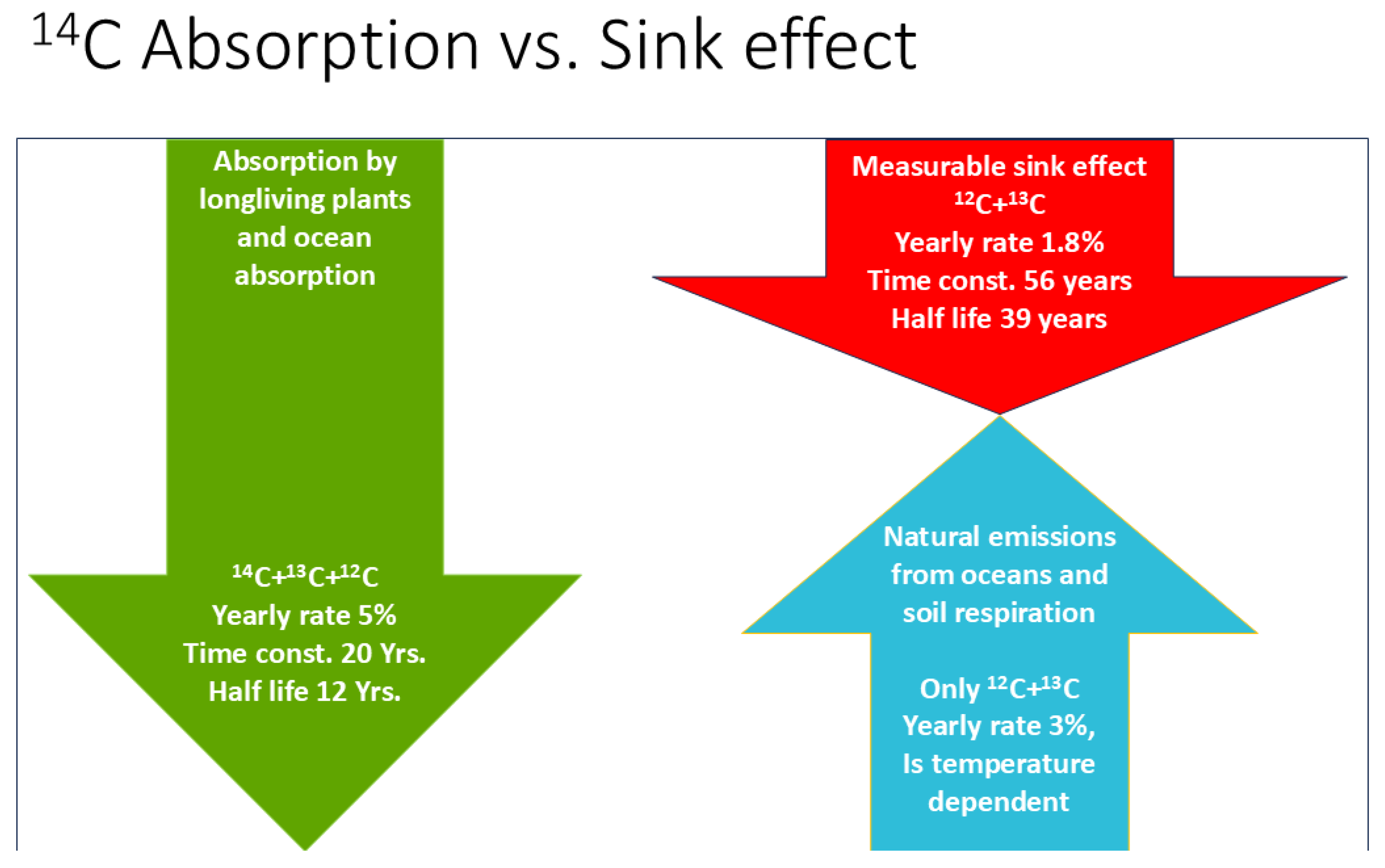
2.2.1. Estimating CO₂ Absorption by Means of the Bomb Test Data

The nuclear bomb tests beginning in the 1950s stopped rather suddenly in 1963 with the nuclear test ban treaty. This provides a close-to-ideal identifiable carbon emission pulse of ¹⁴C that has been thoroughly investigated for more than 40 years [13]. The data series is the global data sequence from 1950 to 2019 from the supplements of [13]. The relative deviation from the preindustrial zero level of ¹⁴C concentration, Δ¹⁴C, is displayed as the blue graph in Figure 2.

Why is this concentration decay representing “pure” absorptions? The ${\mathrm{CO}}_2$ emissions from the oceans have the much lower ¹⁴C concentration of the long-term equilibrium before the bomb tests; therefore, the upwelling ¹⁴C can be neglected.

The primary purpose of the publication from Hua et al. [13] was to provide a data set usable for correcting carbon dating measurements. Therefore, the zero concentration reference level is the preindustrial level before 1900. The purpose here, however, is a completely different one. We want to determine the time constant of the atmospheric decay of ${\Delta }^{14}$C caused by ocean sinks and long-living plants. Therefore, we have to preprocess the data by treating the ${}^{14}C$ dilution in the atmosphere caused by fossil fuels that do not contain ${}^{14}C$, the so-called Suess effect [26], in a different way than required by carbon dating.

In order to deal with the Suess effect properly, we need to look at the definition of the provided data. They are calculated in the ${\Delta }^{14}C$ convention [27,28,29], which is defined as follows:

$${\Delta }^{14}C\left(t\right)=\left({\displaystyle \frac{{}^{14}C_{Atm}\left(t\right){/}^{12}C\left(t\right)}{{}^{14}C_{Std}{/}^{12}{C}_{Std}}}-1\right)·1000$$

(18)

${\Delta }^{14}C\left(t\right)$ are the relative deviations from the pre-industrial reference concentration level of ${}^{14}C$. This contains all deviations from the pre-industrial standard, both the Suess effect and the bomb test anomaly. But because we want to model the post-bomb test ¹⁴C data as an exponential decay, the fact that the ${\Delta }^{14}C\left(t\right)$ data are negative in the years before the bomb tests due to the Suess effect requires an adjustment. In the definition of ${\Delta }^{14}C\left(t\right)$, the pre-industrial zero level had been fixed in order to meet the needs of carbon dating, but in order to measure the decay of the bomb test ¹⁴C concentration, the zero level has to be the level just before the bomb test, that is, just before the sharp rise.

The resulting decreasing atmospheric ¹⁴C concentration shows, over a more than 40-year time period, that the contributing absorption sink processes exhibit an undistorted exponential decay of a first-order linear differential equation; see Figure 3.

This decay includes both the decay of ¹⁴C concentration into the sinks and the Suess effect due to atmospheric concentration change of ¹²C by anthropogenic emissions. For the determination of the Suess effect, we take the 25 years from 1965 to 1990, where we have a good ¹⁴C decay signal.

The upper bound of the diluting Suess effect due to fossil fuels is obtained by pretending there is no sink effect, thus adding the cumulative emissions of 60 ppm (=127 GtC) between 1965 and 1990 to the 1965 ${\mathrm{CO}}_2$ concentration of 320 ppm. The yearly diluting contribution is calculated by

$$\Delta C_{Suess}=\sqrt[25]{{\displaystyle \frac{320+60}{320}}}=1.0069$$

This means that the Suess effect contributes 0.69% per year to the decline of ${\Delta }^{14}C$. The regression parameter for the slope in Figure 3 is −0.058, with the 95% confidence interval [−0.054, −0.063]. When this is reduced by 0.0069, the real absorption constant of ¹⁴C is −0.051, with a corresponding confidence interval. This means that around 5.1% of the surplus ¹⁴C is absorbed by oceans and long-living plants each year. The 5.1% corresponds to a time constant of 19 years, which is close to and definitively within the error range—the value that was also determined by Burton [8,30] based on the data provided from [31].

It is a basic fact of physics that neither absorption into the ocean nor photosynthesis can differentiate between the isotopes ¹⁴C and ¹²C. Therefore, we have to assume that this high rate of absorption applies to all the ${\mathrm{CO}}_2$. This number will have to be related to the result of the extended sink model. The deviation to the measured sink effect must necessarily be caused by natural emissions.

2.2.2. Estimating the Temperature Effect on Natural Emissions from Land Plants and Oceans

As stated above, photosynthesis is the primary driver of the following processes of plant decay and soil respiration. In a recent article, it was confirmed that the Gross Primary Production (GPP) in absolute numbers is 5% larger than soil respiration [6]. In [32], the Net Primary Production (NPP) during the time interval from 1982 to 1999 was investigated. They found a yearly increase of 3.4 GtC of NPP over 18 years. During this time, the temperature increased by 0.25 °C. This would imply a 13.6 GtC increase of bound carbon per °C and year. According to the article, this was not only due to the increase of ${\mathrm{CO}}_2$ fertilization but also, to a large degree, to the reduction of cloud cover over the Amazon rainforest and an increase in solar radiation, which directly influences photosynthetic processes more than ${\mathrm{CO}}_2$ concentration and temperature. A later reported decline of yearly NPP by 0.55 GtC in the years 2000–2009 [33] adjusts this exorbitantly high yearly number to 2.85 GtC/0.5 °C = 5.7 GtC/°C.

According to [34], during the 19 years from 1989 to 2008, the natural emissions from soil respiration $R_S$ have risen by 0.1 GtC per year, i.e., 1.9 GtC during the whole investigation period. During this time, the global temperature has risen by 0.3 °C see, e.g., Figure 4. Therefore, we have a temperature dependency of $R_S$ per year:

$${\displaystyle \frac{\Delta R_S}{\Delta T}}={\displaystyle \frac{1.9}{0.3}}\mathrm{GtC}/°\mathrm{C}=6.33\mathrm{GtC}/°\mathrm{C}$$

An $R_S$ increase of 3.3 GtC/°C per year is reported by [35]. According to [36], there is considerable uncertainty in the determination of the temperature sensitivity of soil respiration.

Regarding the temperature dependence of the emissions from the oceans, we begin with the baseline of yearly emissions from oceans of 80–100 GtC [1]. According to [37], the relative change in ${\mathrm{CO}}_2$ partial pressure in seawater is 0.0423 per °C for a wide range of temperatures from 2 °C to 28 °C. Therefore, the yearly increase in terms of absolute mass would be in the range between 80 GtC · 0.042/°C = 3.4 GtC/°C and 100 GtC · 0.042/°C = 4.2 GtC/°C. It is noteworthy that F. Engelbeen in the “Conclusions” of [9] agrees in principle with yearly rates ranging from 3 to 5 GtC/°C, but he restricts the validity of this process to just a few subsequent years, most likely as a consequence of his assumption that the temperature time derivative is the driving parameter, an assumption I do not share.

Adding the collected evidence for temperature dependency of both soil respiration and ocean emissions results in a total range from 3.3 + 3.4 = 6.7 GtC/°C to 6.3 + 4.2 = 10.5 GtC/°C per year. This is based only on a few investigations, requiring further research. But it gives an indication of what we can realistically expect.

3. Results and Discussion

Since details of the last two years are now relevant, the calculations are performed with monthly data up to December 2024 in order to obtain a clear picture and minimize the effect of boundary conditions. The starting point is the original monthly Mauna Loa measurement time series, which is shown in Figure 5.

The monthly data are subject to seasonal fluctuations caused by the uneven distribution of land mass between the Northern and Southern Hemisphere. Therefore, the first processing step is to remove the seasonal influences, i.e., all periodic changes with a period of 1 year [38]. Due to the 12-month averaging in the Equations (8)–(11), deseasonalization is done implicitly. Only for the purpose of display, deseasonalization has to be done explicitely. Specifically, this was done with a third-order trend component and a cyclical component of sine and cosine terms up to the second order. The details are described in Appendix A. The results of the deseasonalized ${\mathrm{CO}}_2$ concentrations are displayed in Figure 5 (orange color).

The global sea surface temperature is also subject to seasonal fluctuations, but to a much lesser extent, as shown in Figure 4.

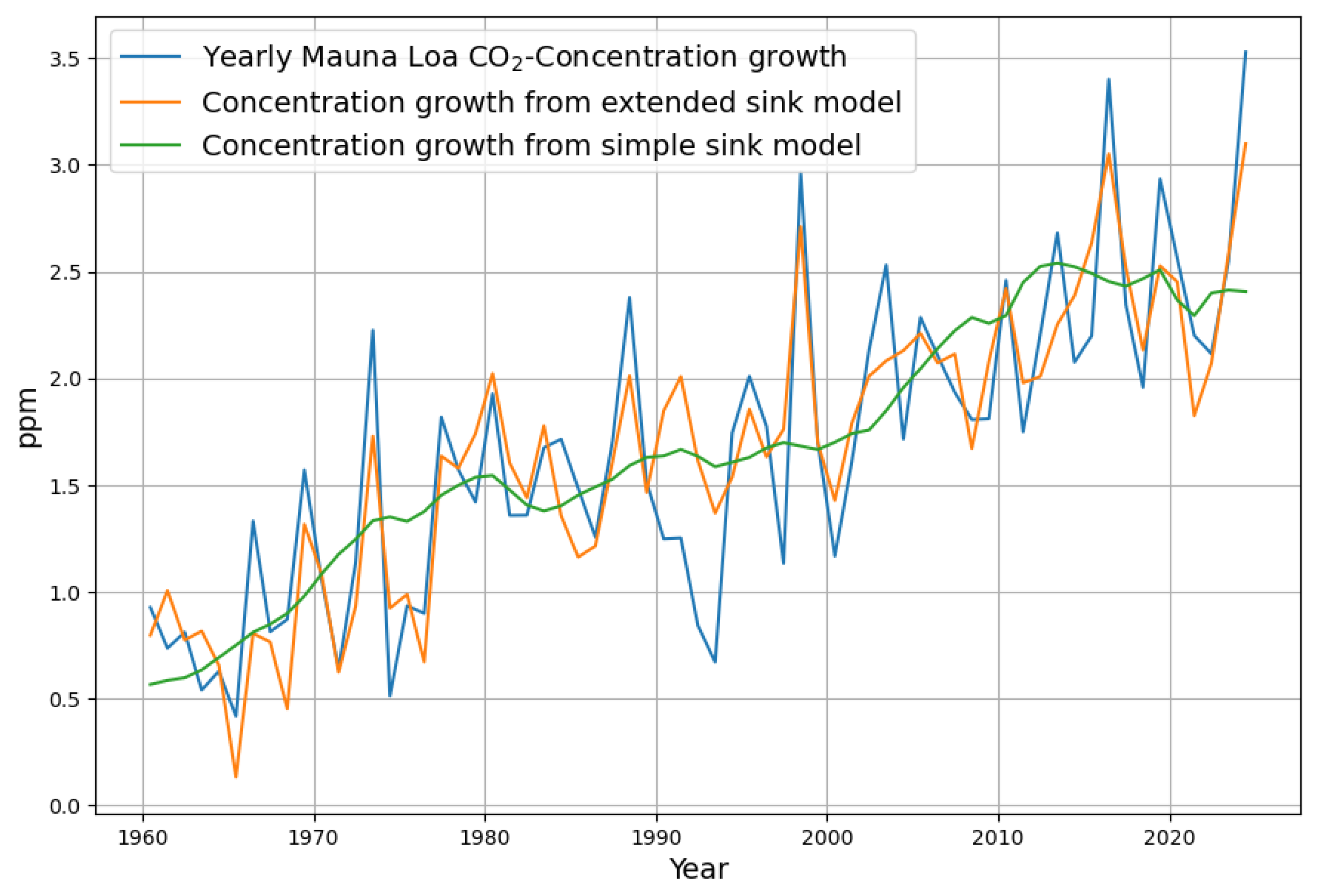
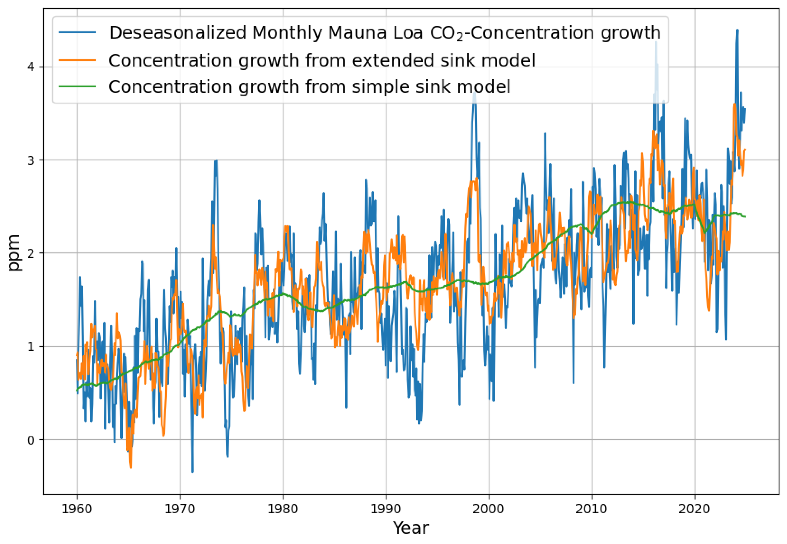
3.1. Formation and Analysis of the Monthly Increase in Concentration

The deseasonalized increase in concentration is calculated according to Equation (11), and the results are displayed in Figure 6.

The monthly fluctuations of concentration growth indicate that the high peak at the end of 2023 is by no means a singular event. In 2016, there was a similarly large spike and a trend of decline until 2022. The 2023 spike is interpreted as a decrease in sink performance in the current media discussion. The diagram, however, shows a gradually increasing trend with similar spikes from time to time.

3.2. Evaluation of the Two Sink Models

Figure 7 shows the effective sink capacity (green) from the difference between anthropogenic emissions (blue) and concentration growth (orange). The sink capacity is displayed with a negative sign in order to separate it visually from the concentration growth. The sink capacity is increasing with time, not decreasing.

It is easy to see that the effective sink capacity does not fall below 0 at the right-hand edge of Figure 7; these rare situations only occurred before 1999. However, it was actually decreasing in 2023–2024.

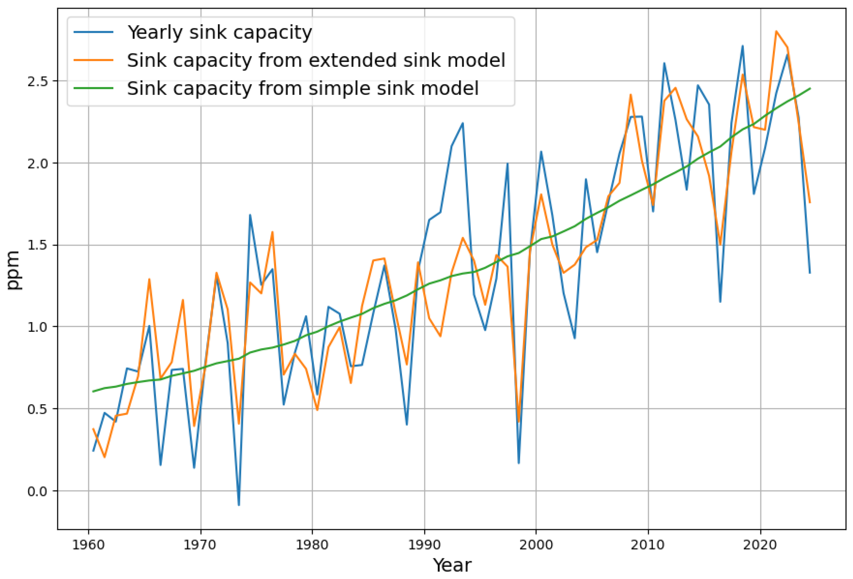
3.2.1. Evaluation with the Simple Concentration-Dependent Sink Model

The design of the simple concentration model has been extended compared to previous papers by allowing a time shift of the ${\mathrm{CO}}_2$ concentration in least squares optimization (Equation (12)). The optimization is conducted for all time shifts between 0 and 22 months. The explained variance ratio $R^2$ of the model is shown in Figure 8. After optimization for the two parameters $a^{\prime }$ and n, the $R^2$ value of the regression has a maximum of nearly 0.59 at the optimal time shift of 16 months. This means that the simple model explains, at most, 59% of the original data variability.

Table 1. Shift and corresponding metrics ($R^2$, $a^{\prime }$, n, and $C^0$).

Metric	Shift
	11	12	13	14	15	16	17	18
$R^2$	0.5880	0.5886	0.5890	0.5895	0.5896	0.5897	0.5896	0.5895
$a^{\prime }$	0.0175	0.0176	0.0176	0.0176	0.0176	0.0177	0.0177	0.0177
n	−4.93	−4.94	−4.95	−4.96	−4.97	−4.97	−4.98	−4.99
$C^0$	282.2	282.7	283.2	283.7	284.1	284.5	284.9	285.2

displays the most relevant time shift dependent values, the explained variance ratio $R^2$, the sink parameter $a^{\prime }$, the model constant n, and the equilibrium ${\mathrm{CO}}_2$ concentration $C^0$.

The estimated model parameters $a^{\prime }$ and n are not very sensitive to the applied time shift, but a maximum of the explained variance is clearly visible. As there are several underlying causal processes involved, the visible maximum is an indication of the most dominant process. Determining the mechanism in nature that causes this time delay is the subject of further research.

With the optimal concentration time shift, the model Equation (4) becomes:

$${\widehat{S}}_i\left(C\right)=0.018·(\sum _{k=12i}^{12i+11}{\displaystyle \frac{1}{12}}{C}_{k-16}^{\mathrm{month}}-285\mathrm{ppm})$$

(19)

The value $C^0=285$ ppm can be interpreted as the effective preindustrial equilibrium concentration. The 95% confidence interval for the absorption parameter $a^{\prime }$ is [0.014, 0.021]. The 95% confidence interval for $C^0$ is [192, 379] and is, therefore, very large. But it is plausible: when the relative error of $a^{\prime }$ is about 10% and the relative error for n is 13%, then the relative error of their ratio is 17%. Therefore, it is not surprising that different authors arrive at different values depending on their data selection and model design.

3.2.2. Evaluation with the Extended Concentration and Temperature-Dependent Sink Model

The extended sink model $\widehat{S}(C,T)$, Equation (14), is replacing $\widehat{S}\left(C\right)$ in the least squares optimization (Equation (12)). Using the ${\mathrm{CO}}_2$ concentration time shift of 16, the optimization is conducted for temperature time shifts from 0 to 12 months. Figure 9 shows that the explained variance ratio $R^2$ has a rather clear maximum of more than 0.8 at a time shift of 4 months. This is a quite remarkable increase in the explained variance ratio, leaving only 20% of the total variance unexplained.

Table 2. Temperature time shift and corresponding metrics in extended sink model ($R^2$, a, b, c, and ${\widehat{C}}^0$).

Metric	Shift
	0	1	2	3	4	5	6	7	8
$R^2$	0.7321	0.7668	0.7902	0.8032	0.8078	0.8033	0.7943	0.7886	0.7755
a	0.0456	0.0484	0.0497	0.0500	0.0497	0.0492	0.0485	0.0481	0.0475
b	−3.12	−3.45	−3.61	−3.66	−3.63	−3.59	−3.51	−3.49	−3.42
c	−14.20	−15.13	−15.58	−15.69	−15.57	−15.42	−15.18	−15.07	−14.85
${\widehat{C}}^0$	311.8	312.9	313.5	313.6	313.5	313.4	313.2	313.1	312.8

displays the dependence of $R^2$, the absorption value a, the temperature coefficient b, the constant c, and the equilibrium concentration ${\widehat{C}}^0$ on the temperature time shift.

With this optimal timeshift, the final extended sink model ${\widehat{S}}_i(C,T)$ is determined:

$${\widehat{S}}_i(C,T)=0.05·(\sum _{k=12i}^{12i+11}{\displaystyle \frac{1}{12}}{C}_{k-16}^{\mathrm{month}}-313.5\mathrm{ppm})-3.63{\displaystyle \frac{\mathrm{ppm}}{{}^{\circ }\mathrm{C}}}·\sum _{k=12i}^{12i+11}{\displaystyle \frac{1}{12}}{T}_{k-4}^{\mathrm{month}}$$

(20)

where $C_k^{\mathrm{month}}$ are the measured monthly Mauna Loa ${\mathrm{CO}}_2$ concentration data [11] and $T_{k-4}^{\mathrm{month}}$ are the timeshifted temperatures computed from monthly HadSST4 sea surface anomalies [12].

The ${\mathrm{CO}}_2$ dependent absorption with 5% is significantly larger than in the simple sink model, where it was 1.8%. At first sight, it is hard to understand how this discrepancy comes about. Therefore, it is visualized with the diagram, Figure 10.

The measured sink effect from Equation (2) can be approximated directly with a linear function depending on the ${\mathrm{CO}}_2$ concentration. This is represented by the simple sink model with the red arrow. It can also be represented by two processes: downwelling large absorption, represented by the green arrow, and upwelling natural emissions, represented by the blue arrow. The blue arrow partly compensates for the effect of the green arrow. The fact that these upwelling natural emissions are temperature-dependent makes them identifiable when including temperature in the model.

Figure 11 shows the resulting sink effect of both the simple sink model and the extended model in comparison with the measured sink data. While the simple sink model represents the trend of the data, the extended model follows the short-term deviations of 1 to 4 years very well. There is one noteworthy exception. After 1991, there was a remarkable rise in the sink rate, which has no correspondence with the model variability caused by temperature. The reason has been described by Roy Spencer [7], who writes, “Significant model departures from observations occurred for three years after the 1991 eruption of Mt. Pinatubo” and explains it as a consequence of increased photosynthesis due to more diffuse solar radiation.

3.3. Comparing the Absorption Rate of the Extended Sink Model with the Decay Rate of the Bomb Test Data

According to Equation (20), the extended sink model has the result that the yearly absorptions are rather large, approximately 5% of the ${\mathrm{CO}}_2$ concentration beyond the equilibrium concentration, which is partly compensated by a significantly large effect of temperature dependence on natural emissions, approximately 3.6 ppm/°C (7.7 GtC/°C) per year. The 95% confidence interval of the absorption rate is [0.042, 0.058].

The decay rate of bomb test data with the Suess effect correction is 5.1% per annum. This rate matches very closely the determined absorption rate by the extended sink model within the statistical error boundaries. This supports the ability of the extended sink model to separate natural absorptions from natural emissions instead of mixing them as in the simple sink model. The absorption rate is, therefore, only controlled by the ${\mathrm{CO}}_2$ concentration, while natural emissions are controlled by sea surface temperature.

3.4. Comparing the Temperature Coefficient of the Extended Model with the Empirical Natural Emissions

The possible range of natural emissions temperature dependency was determined in Section 2.2.2 to be in the range of between 6.7 GtC/°C per year and 10.5 GtC/°C per year. With the temperature coefficient of the extended model, the value 3.6 ppm/°C = 7.7 GtC/°C with the 95% confidence interval [5.9, 9.5] GtC/°C can be considered as a very good match.

Therefore, the empirically determined rates of temperature dependency are a good confirmation for the extended sink model.

3.5. Reconstruction of the Concentration Growth from Both Sink Models

The calculations show clearly that the concentration-dependent absorptions of oceans and land plants have not changed at all, but that the natural emissions have increased due to temperature increases.

How is this reflected in the model-based reconstruction of the concentration growth? Figure 12 shows what the inclusion of temperature means for modeling the yearly concentration growth.

While the green curve represents the widely known concentration-based simple sink model, the orange curve also takes into account the dependence on temperature, as described. It turns out that the current large increase in concentration growth is a natural consequence of the underlying rise in temperature. While the green curve of the concentration-dependent model predicts a decrease in concentration growth for 2023 and 2024, the extended sink model follows nicely the actual rising concentration growth values.

The monthly concentration growth is also reconstructed by the two models as shown in Figure 13. Also in the monthly resolution, the temperature model matches very well the variability of the measured data.

4. Conclusions

The continuity equation, together with the observed consistent decrease in the ¹⁴C concentration in the atmosphere after 1963 and the observation of temperature-dependent natural emissions, are powerful tools for evaluating observations.

One purpose of this article is to explain the recent rise in concentration growth as a consequence of rising sea surface temperatures instead of a hypothetical unobserved decline in absorption by oceans or plants. While the rise in concentration growth is real, the cause is not a failure of sinks but a larger rise in temperature beyond the trend that corresponded to ${\mathrm{CO}}_2$ level rise.

It should, therefore, not be off-limits to consider temperature as a “normal” cause of ${\mathrm{CO}}_2$ concentration changes in the public debate, as an influencing factor instead of speculating about the absence of sinks without evidence.

This does not exclude a causality in the other direction; the greenhouse effect, the rather large temperature coefficient on natural ${\mathrm{CO}}_2$ emissions, certainly limits the possible climate sensitivity.

Regarding causality, the first climate-relevant test of the temperature-dependent model was made on the VOSTOK ice-core data [10], where there were no anthropogenic emissions and the ${\mathrm{CO}}_2$ concentration of the last 400,000 years was modeled from preceding temperature data.

The temperature-dependent model makes it possible to separate better between the actual anthropogenic origin of ${\mathrm{CO}}_2$ changes and the natural causes, among which temperature is a very important one. Many people were confused when, in 2020, no effect of the anthropogenic emission reduction could be seen in the concentration growth. When the temperature effect is removed, as is the case in the simple model, then the effect of the lockdown-caused emission reduction can be seen, e.g., the green curve in Figure 12.

The most important contribution is that it became possible to separate downwelling absorptions from upwelling natural emissions. Through the evaluation of the bomb test ¹⁴C time series and by the Suess effect correction, we have a reliable estimate of the yearly absorption rate as 5% of the ${\mathrm{CO}}_2$ concentration. Together with the precise ${\mathrm{CO}}_2$ concentration measurements on Mauna Loa and the accepted measurements of anthropogenic emissions from the International Energy Agency (IEA), the continuity Equation (1) constrains the yearly net natural emissions. Together with the extended model, we also have an understanding of their temperature dependency.

Some misunderstandings and misconceptions are challenged by the discussed concepts.

• The most obvious is the argument of some climate skeptics that anthropogenic emissions have no effect because they are apparently “drowned” in the huge natural carbon cycle. The fact is that anthropogenic emissions are a direct cause of concentration growth. Nature behaves as a strict net sink. This is obvious from Figure 7. Both models ended up with a significant, consistent net sink effect for the last 70 years when reliable data were available. Therefore, anthropogenic emissions must have significantly contributed to the total concentration growth. The extended model can hypothetically switch off the variability of natural emissions by setting the parameter for the temperature to 0. Alternatively, the anthropogenic emissions can be set to an arbitrary constant value so that only the temperature-controlled natural emissions control the ${\mathrm{CO}}_2$ concentration growth.
• Natural emissions by gardens, animals, and even agriculture, in general, are increasingly becoming a political target. As discussed, increasing natural emissions from biota are almost always a secondary consequence of a previous increase in photosynthesis and, therefore, NPP. But they are only a fraction of NPP. Therefore, extreme care has to be taken not to create more harm than good by carbon-related political interference with biota or agriculture. Mechanical agriculture and chemical contributions to agriculture are already accounted for by the measured anthropogenic emissions. It is, therefore, not legitimate to count them twice by attaching their effect to the biological product.
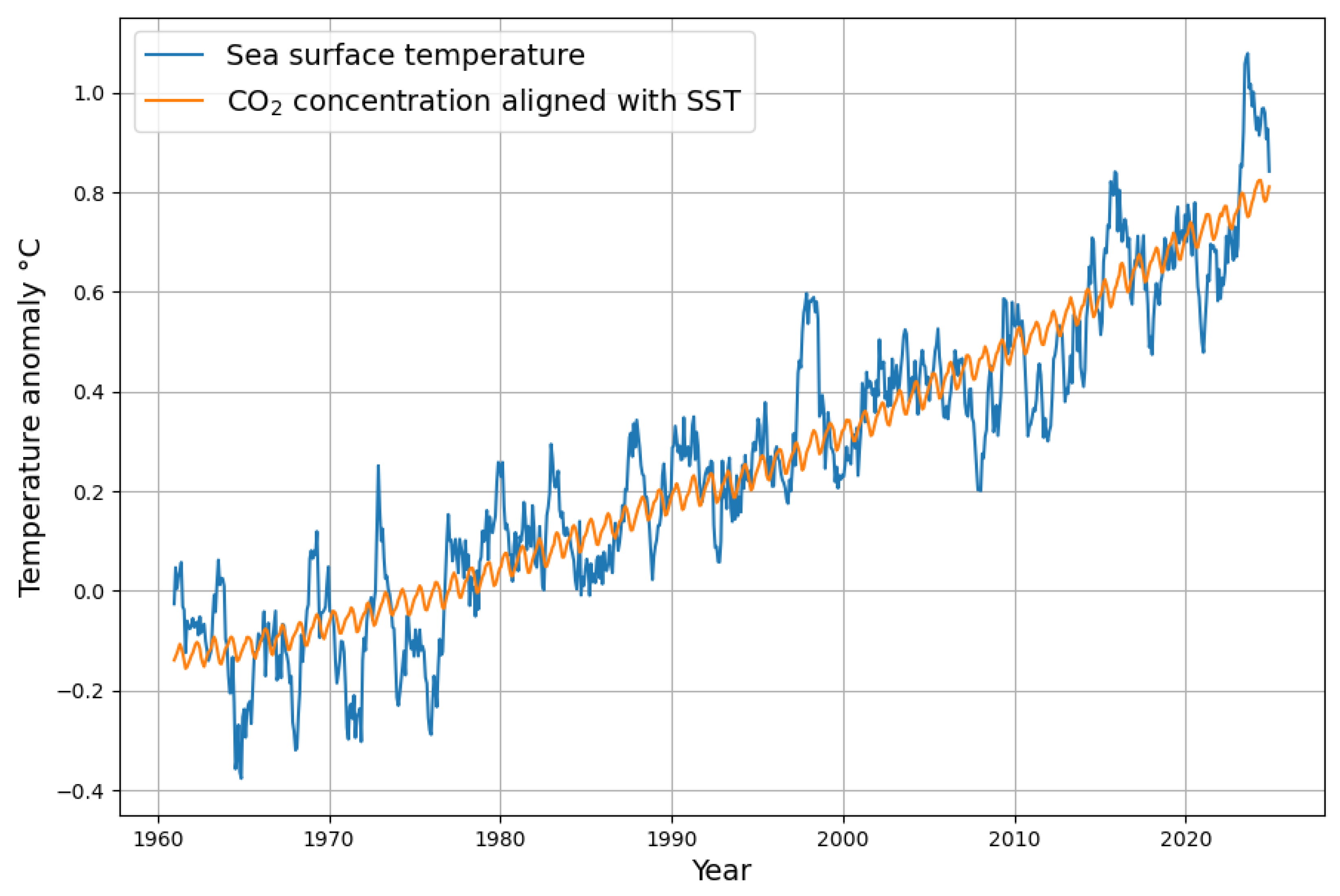
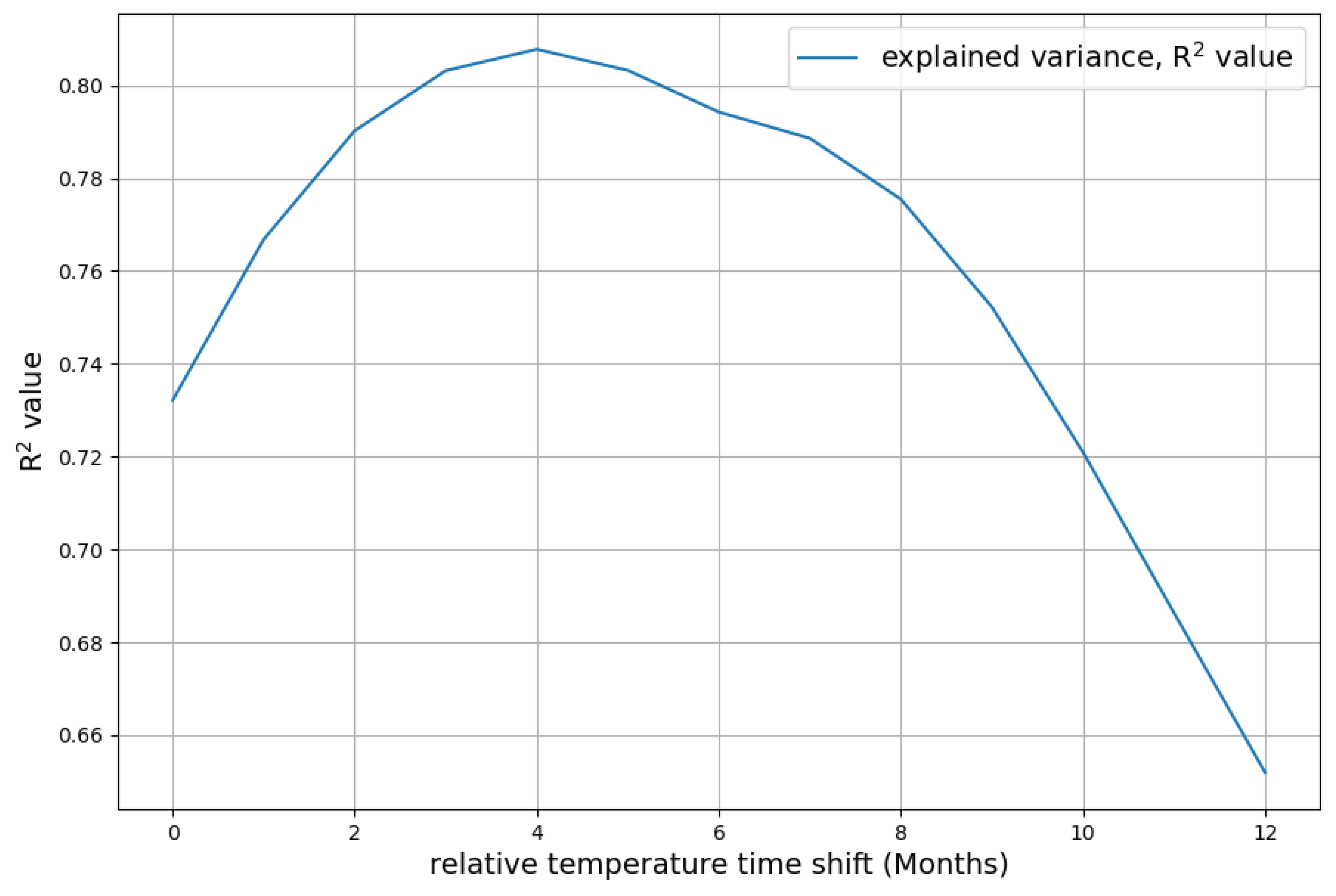
• The necessary time shift, where temperature change precedes changes in concentration change, is a clear statement of causality that, to a certain degree, ${\mathrm{CO}}_2$ concentration change follows temperature. Climate models should include this causality and honestly face the consequences. The most dramatic is that it leads in a natural way to a much higher absorption rate of the sink system than the currently accepted value.

Of course, questions for further research remain. Due to the fact that the continuity equation must hold at all time scales, we expect new insights about the carbon cycle from systematically investigating multiple timescales and the behavior of model parameters.

References

1. Friedlingstein, P.; O’Sullivan, M.; Jones, M.W.; Andrew, R.M.; Bakker, D.C.E.; Hauck, J.; Landschützer, P.; Le Quéré, C.; Luijkx, I.T.; Peters, G.P.; et al. Global Carbon Budget 2024. Earth Syst. Sci. Data Discuss. 2024, 2024, 1–133. [Google Scholar] [CrossRef]
2. Ke, P.; Ciais, P.; Sitch, S.; Li, W.; Bastos, A.; Liu, Z.; Xu, Y.; Gui, X.; Bian, J.; Goll, D.S.; et al. Low latency carbon budget analysis reveals a large decline of the land carbon sink in 2023. Natl. Sci. Rev. 2024, 11, nwae367. [Google Scholar] [CrossRef] [PubMed]
3. Bunsen, F.; Nissen, C.; Hauck, J. The Impact of Recent Climate Change on the Global Ocean Carbon Sink. Geophys. Res. Lett. 2024, 51, e2023GL107030. [Google Scholar] [CrossRef]
4. Ruehr, S.; Keenan, T.F.; Williams, C.; Zhou, Y.; Lu, X.; Bastos, A.; Canadell, J.G.; Prentice, I.C.; Sitch, S.; Terrer, C. Evidence and attribution of the enhanced land carbon sink. Nat. Rev. Earth Environ. 2023, 4, 518–534. [Google Scholar] [CrossRef]
5. Arora, V.K.; Katavouta, A.; Williams, R.G.; Jones, C.D.; Brovkin, V.; Friedlingstein, P.; Schwinger, J.; Bopp, L.; Boucher, O.; Cadule, P.; et al. Carbon-concentration and carbon-climate feedbacks in CMIP6 models and their comparison to CMIP5 models. Biogeosciences 2020, 17, 4173–4222. [Google Scholar] [CrossRef]
6. Lai, J.; Kooijmans, L.M.J.; Sun, W.; Cho, A.; Xu, L.; Vesala, T.; Krol, M.C.; van der Laan-Luijkx, I.T.; Keronen, P.; Wofsy, S.C.; et al. Terrestrial photosynthesis inferred from plant carbonyl sulfide uptake. Nature 2024, 634, 855–861. [Google Scholar] [CrossRef] [PubMed]
7. Spencer, R.W. ENSO Impact on the Declining CO2 Sink Rate. J. Mar. Sci. Res. Oceanogr. 2023, 6, 163–170. [Google Scholar] [CrossRef]
8. Engelbeen, F.; Hannon, R.; Burton, D. The Human Contribution to Atmospheric Carbon Dioxide. 2024. Available online: https://co2coalition.org/wp-content/uploads/2024/12/Human-Contribution-to-Atmospheric-CO2-digital-compressed.pdf (accessed on 15 June 2025).
9. Engelbeen, F. The Origin of the Increase of CO2 in the Atmosphere. 2022. Available online: http://www.ferdinand-engelbeen.be/klimaat/co2_origin.html (accessed on 15 June 2025).
10. Dengler, J. Improvements and Extension of the Linear Carbon Sink Model. Atmosphere 2024, 15, 743. [Google Scholar] [CrossRef]
11. NOAA. Trends in Atmospheric Carbon Dioxide (CO2). 2023. Available online: https://gml.noaa.gov/ccgg/trends/data.html (accessed on 15 June 2025).
12. Kennedy, J.J.; Rayner, N.A.; Atkinson, C.P.; Killick, R.E. An ensemble data set of sea-surface temperature change from 1850: The Met Office1 Hadley Centre HadSST.4.0.0.0 data set. J. Geophys. Res. Atmos. 2019, 124, 7719–7763. [Google Scholar] [CrossRef]
13. Hua, Q.; Turnbull, J.C.; Santos, G.M.; Rakowski, A.Z.; Ancapichun, S.; De Pol-Holz, R.; Hammer, S.; Lehman, S.J.; Levin, I.; Miller, J.B.; et al. Atmospheric Radiocarbon for the Period 1950–2019. Radiocarbon 2022, 64, 723–745. [Google Scholar] [CrossRef]
14. Dengler, J.; Reid, J. Emissions and CO2 Concentration—An Evidence Based Approach. Atmosphere 2023, 14, 566. [Google Scholar] [CrossRef]
15. Dietze, P. Carbon Model Calculations. 2001. Available online: https://web.archive.org/web/20250305084230/http://www.john-daly.com/dietze/cmodcalc.htm (accessed on 15 June 2025).
16. Halparin, A. Simple Equation of Multi-Decadal Atmospheric Carbon Concentration Change. 2015. Available online: https://defyccc.com/docs/se/MDACC-Halperin.pdf (accessed on 15 June 2025).
17. Dübal, H.; Vahrenholt, F. Oceans’ surface pH-value as an example of a reversible natural response to an anthropogenic perturbation. Ann. Mar. Sci. 2023, 7, 034–039. [Google Scholar] [CrossRef]
18. Vollmer, M.; Eberhardt, W. A simple model for the prediction of CO2 concentrations in the atmosphere, depending on global CO2 emissions. Eur. J. Phys. 2024, 45, 025803. [Google Scholar] [CrossRef]
19. Seabold, S.; Perktold, J. Statsmodels: Econometric and statistical modeling with python. In Proceedings of the 9th Python in Science Conference, Austin, TX, USA, 28 June–3 July 2010. [Google Scholar]
20. Hunter, J.D. Matplotlib: A 2D graphics environment. Comput. Sci. Eng. 2007, 9, 90–95. [Google Scholar] [CrossRef]
21. Meacham-Hensold, K. The Difference Between C3 and C4 Plants. 2020. Available online: https://ripe.illinois.edu/blog/difference-between-c3-and-c4-plants (accessed on 15 June 2025).
22. Haverd, V.; Smith, B.; Canadell, J.G.; Cuntz, M.; Mikaloff-Fletcher, S.; Farquhar, G.; Woodgate, W.; Briggs, P.R.; Trudinger, C.M. Higher than expected CO2 fertilization inferred from leaf to global observations. Glob. Change Biol. 2020, 26, 2390–2402. [Google Scholar] [CrossRef]
23. Humlum, O.; Stordahl, K.; Solheim, J.E. The phase relation between atmospheric carbon dioxide and global temperature. Glob. Planet. Change 2013, 100, 51–69. [Google Scholar] [CrossRef]
24. Richardson, M. Comment on “The phase relation between atmospheric carbon dioxide and global temperature” by Humlum, Stordahl and Solheim. Glob. Planet. Change 2013, 107, 226–228. [Google Scholar] [CrossRef]
25. Wolter, K.; Timlin, M.S. El Ni n ˜ o/Southern Oscillation behaviour since 1871 as diagnosed in an extended multivariate ENSO index (MEI.ext). Int. J. Climatol. 2011, 31, 1074–1087. [Google Scholar] [CrossRef]
26. Suess, H.E. Radiocarbon Concentration in Modern Wood. Science 1955, 122, 415–417. [Google Scholar] [CrossRef]
27. Levin, I.; Kromer, B.; Schoch-Fischer, H.; Bruns, M.; Münnich, M.; Berdau, D.; Vogel, J.C.; Münnich, K.O. 25 Years of Tropospheric 14C Observations in Central Europe. Radiocarbon 1985, 27, 1–19. [Google Scholar] [CrossRef]
28. Stuiver, M.; Polach, H.A. Discussion Reporting of 14C Data. Radiocarbon 1977, 19, 355–363. [Google Scholar] [CrossRef]
29. Stuiver, M.; Quay, P. Atmospheric14C changes resulting from fossil fuel CO2 release and cosmic ray flux variability. Earth Planet. Sci. Lett. 1981, 53, 349–362. [Google Scholar] [CrossRef]
30. Burton, D.A. Comment on Stallinga, P. (2023), Residence Time vs. Adjustment Time of Carbon Dioxide in the Atmosphere. 2024. Available online: https://osf.io/preprints/osf/brdq9_v2 (accessed on 15 June 2025).
31. Graven, H.; Keeling, R.F.; Rogelj, J. Changes to Carbon Isotopes in Atmospheric CO2 Over the Industrial Era and Into the Future. Glob. Biogeochem. Cycles 2020, 34, e2019GB006170. [Google Scholar] [CrossRef]
32. Nemani, R.R.; Keeling, C.D.; Hashimoto, H.; Jolly, W.M.; Piper, S.C.; Tucker, C.J.; Myneni, R.B.; Running, S.W. Climate-Driven Increases in Global Terrestrial Net Primary Production from 1982 to 1999. Science 2003, 300, 1560–1563. [Google Scholar] [CrossRef]
33. Zhao, M.; Running, S.W. Drought-Induced Reduction in Global Terrestrial Net Primary Production from 2000 Through 2009. Science 2010, 329, 940–943. [Google Scholar] [CrossRef] [PubMed]
34. Bond-Lamberty, B.; Thomson, A. Temperature-associated increases in the global soil respiration record. Nature 2010, 464, 579–582. [Google Scholar] [CrossRef]
35. Hashimoto, S.; Carvalhais, N.; Ito, A.; Migliavacca, M.; Nishina, K.; Reichstein, M. Global spatiotemporal distribution of soil respiration modeled using a global database. Biogeosciences 2015, 12, 4121–4132. [Google Scholar] [CrossRef]
36. Davidson, E.A.; Janssens, I.A. Temperature sensitivity of soil carbon decomposition and feedbacks to climate change. Nature 2006, 440, 165–173. [Google Scholar] [CrossRef]
37. Takahashi, T.; Olafsson, J.; Goddard, J.G.; Chipman, D.W.; Sutherland, S.C. Seasonal variation of CO2 and nutrients in the high-latitude surface oceans: A comparative study. Glob. Biogeochem. Cycles 1993, 7, 843–878. [Google Scholar] [CrossRef]
38. Brownlee, J. How to Identify and Remove Seasonality from Time Series Data with Python. 2020. Available online: https://machinelearningmastery.com/time-series-seasonality-with-python/ (accessed on 15 June 2025).
Figure 1. Sea surface temperature, original (blue) [12]. Temperature modeled with CO 2 (orange) [11].
Applsci 15 06907 g001
Figure 2. The decay of the global atmospheric Δ 14 C after 1965 [13]. Published data are blue, and adjusted data are orange.
Applsci 15 06907 g002
Figure 3. Determination of the 14C decay rate by a logarithmic transformation.
Applsci 15 06907 g003
Figure 4. Monthly global sea surface temperature time series [12] and deseasonalized monthly global sea surface temperature data.
Applsci 15 06907 g004
Figure 5. Monthly Mauna Loa time series of CO 2 concentration (blue) [11] and deseasonalized monthly CO 2 concentration data (orange).
Applsci 15 06907 g005
Figure 6. Monthly deseasonalized concentration growth.
Applsci 15 06907 g006
Figure 7. Anthropogenic emissions (blue) [1], CO 2 deseasonalized concentration growth (orange), and corresponding sink capacity (green). The sink capacity after 2000 is always larger than 0, and it has an approximately linear increasing trend. In 2023 and 2024 there is a reduction to nearly 0. This corresponds with a rise in concentration growth nearly reaching the anthropogenic emissions. Such situations occurred multiple times in the past.
Applsci 15 06907 g007
Figure 8. Explained variance of simple sink model as a function of CO 2 concentration shift l a g C , measured in months.
Applsci 15 06907 g008
Figure 9. Explained variance of the extended model as a function of temperature shift, measured in months.
Applsci 15 06907 g009
Figure 10. Composition of the measured sink effect (red) by absorptions (green) and natural emissions (blue).
Applsci 15 06907 g010
Figure 11. Sink effect of averaged monthly data (blue): results of simple sink model (green) and extended sink model (orange).
Applsci 15 06907 g011
Figure 12. Concentration growth of averaged monthly data (blue) and its modeling with the simple sink model (green) and temperature-dependent extended sink model (orange).
Applsci 15 06907 g012
Figure 13. Monthly concentration growth (blue) and its modeling with simple sink model (green) and temperature-dependent extended sink model (orange).
Applsci 15 06907 g013