ANN-Based Real-Time Prediction of Heat and Mass Transfer in the Paper-Based Storage Enclosure for Sustainable Preventive Conservation

Abstract

The storage enclosures are vital for stabilizing the micro-environment within, facilitating preventive conservation efforts, and enabling energy savings by reducing the need for extensive macro-environmental control within the room. However, real-time conformity monitoring of the micro-environment to ensure compliance with preventive conservation specifications poses a practical challenge due to a limitation in implementing physical sensors for each enclosure. This study aims to address this challenge by using an ANN (Artificial Neural Network)-based prediction for temperature and RH (Relative Humidity) changes in response to macro-environmental fluctuations. A numerical model was developed to simulate transient heat and mass transfer between macro- and micro-environments and then employed to determine an acceptable macro-environmental range for sustainable preventive conservation and to generate a dataset to train a sequence-to-sequence ANN model. This model was specially designed for 24 h real-time prediction of heat and mass transfer and to simulate the micro-environmental conditions under varying levels of control accuracy over the macro-environment. The effectiveness of the prediction model was tested through a real trial application in the laboratory, which revealed a robust prediction of micro-environments inside different enclosures under various macro-environmental conditions. This modeling approach offers a promising solution for monitoring the micro-environmental conformity and further implementing the relaxing control strategy in the macro-environment without compromising the integrity of the collections stored inside the enclosures.

1. Introduction

Preventive conservation of heritage collections plays an important role in minimizing climate-induced decay and avoiding detrimental effects when they are maintained in an indoor environment as stable as possible [1]. As many of these collections are composed of organic materials such as paper, which shrink and expand with dropping and rising moisture content, especially fluctuations in relative humidity (RH), they should be avoided to prevent mechanical damage at a fast strain rate in the storage space of libraries, galleries, and museums [2]. Climate change exacerbates this risk, accelerating degradation, increasing conservation costs, and making climatization necessary [3]. While maintaining a stable environment is essential, it requires precision air conditioning with tight control, resulting in substantial energy consumption and carbon emissions [4,5]. Effective conservation and protection of heritage collections require well-informed management tools grounded in an understanding of how environmental parameters evolve over time and vary across the environment [6]. In addition, a great number of collections are usually stored in some European historic buildings with poor energy performance, posing a challenge for retrofitting the buildings where exterior façades are decorated with carvings and sculptures, while interior walls are decorated with frescoes [7]. Consequently, improving operational energy efficiency is a challenging task for achieving sustainable preventive conservation.

Many approaches have been developed for controlling the micro-environment within enclosures rather than the whole macro-environment in the room. Adding some buffering materials inside the enclosures to achieve passive control is a prevalent approach [8]. The enclosure separates the micro-environment inside from the macro-environment, and the room where the enclosure is present and the confined space with buffering materials provide a degree of hygrothermal buffering effect.

In the National Library of Scotland (NLS), the paper-based enclosures are used for storing books in storage rooms, like many other cultural institutions. These enclosures are created from functional cardboard with specific elements and a porous structure. The cardboard consists of three layers: an external waterproof layer, a middle multi-thin layer, and an internal lining layer. The external layer contains polypropylene to provide waterproof and thermal-insulation functions [9,10]. The middle and inner layers contain pulp cotton and calcium carbonate to regulate the micro-environmental temperature and humidity [11,12]. To consider fabric permeability, a thin multi-layer structure is designed in the middle layer to increase the tortuosity of porous channels. This design can increase moisture retention through small air gaps between these layers, thus improving the buffering effect [13].

The enclosures can stabilize the micro-environment, especially mitigating fluctuations in RH due to their buffering effect. This buffering effect has been rigorously evaluated in a laboratory test [14]. It quantified the enclosure’s capacity to minimize the micro-environmental fluctuations over some given periods under two distinct macro-environmental conditions (10 %RH fluctuation within 50~60 %RH at a fixed 20 °C for the humidity buffering test; 5 °C fluctuation within 17~22 °C at a fixed 50 %RH for the temperature buffering test). The results demonstrated that the micro-environmental fluctuations are 2–8 %RH and 1–2 °C smaller than the macro-environmental ones. These findings suggested that the enclosures can provide a degree of buffering capacity to mitigate micro-environmental fluctuation by reducing their response to that of the macro-environment. Such buffering capacity enables a relaxing control for macro-environment when the micro-environment complies with the standards of preventive conservation. This observation aligns with a key insight from an Italian study [15], suggesting that the control accuracy of precision air conditioning systems can be relaxed within the macro-environment, while still ensuring effective preventive conservation within the micro-environment. However, achieving real-time conformity monitoring of the micro-environment to ensure compliance with preventive conservation specifications is constrained by the practical difficulty of implementing a multitude of physical sensors inside the enclosures to map their conditions.

Numerical models that simulate heat and mass transfer between macro- and micro-environments can predict the micro-environment in response to the macro-environment. This technique has been proven effective for conducting hygrothermal analysis [16]. It was used to develop a model to simulate coupled diffusive heat and mass transfer between hygroscopic building structure and indoor air. The model was used to investigate the indoor humidity and air quality in a timber house after its validation with a set of field measurement data [17]. Additionally, based on this technique, a full dynamic hygrothermal model was developed to couple heat and moisture transfer in porous building materials to predict the hygrothermal performance of buildings while incorporating convection and advection [18]. These models excel in capturing hygrothermal interaction between the micro- and macro-environments with good representations of the physical principles. Their application not only enhances understanding of the hygrothermal interaction but also establishes a foundation for assessing the conformity of preventive conservation within the micro-environment and further achieving the relaxed control of the macro-environment.

However, the heat and mass simulation is highly time-consuming, typically running in hours, so it is not feasible to use it practically in precision air conditioning systems with a feedback control loop that operates on a scale of minutes. To address this issue, an artificial neural network (ANN) offers a feasible solution when it is trained with a purposely prepared dataset. This approach has seen successful application in various domains of thermal science. A mathematical model of the refrigerant cycle was created to generate data regarding evaporator cooling capacity and relevant parameters such as airflow, temperature, and RH. Subsequently, this data was used for training the ANN model [19]. Similarly, in a study about the structure optimization of latent heat thermal storage units, computational fluid dynamic simulations were used to describe the transient thermal behavior. Based on the simulation results, an ANN was trained to predict stored energy [20]. Additionally, ANN models trained with historical real data have been instrumental in optimizing building energy use with acceptable indoor microclimate [21].

The above studies show that ANN is an effective tool for capturing the complex operating characteristics of building systems. However, there are only several studies that investigate the hygrothermal interaction in the realm of building science by integrating traditional mathematical modeling with ANN. Remarkably, no prior study has delved into exploring the buffering effect of the storage enclosures in facilitating a relaxing control of macro-environment for sustainable preventive conservation. Therefore, this study aims to achieve real-time conformity monitoring of micro-environment as macro-environmental control is relaxed. To achieve the aim, there are three objectives:

• to develop a coupled heat and mass transfer model for predicting the micro-environment.
• to determine an acceptable macro-environment for obtaining the associated range of the relaxing control.
• to train an ANN model for real-time conformity monitoring of the micro-environment.

2. Methodology

In alignment with these three stated objectives, the methodology framework comprised three parts. First, a numerical model was developed to simulate the heat and mass transfer between the two environments: the macro and micro-environment were validated after. Second, a three-stage method based on the heat and mass transfer simulation was employed to determine the upper limit of acceptable macro-environmental conditions through a trial-and-error process. Following this, a series of simulations was run to acquire data representing conditions under the relaxing control. In the third part, four distinct sets of data were generated within this acceptable range to capture the main characteristics of heat and mass transfer interaction between macro- and micro-environments under relaxed control. Leveraging these generated datasets alongside on-site collected data for tight control, a Long Short-Term Memory (LSTM) neural network was trained for real-time prediction of micro-environmental conditions. Subsequently, the robustness of this real-time prediction was assessed in a practical application. Further details of these activities are provided below.

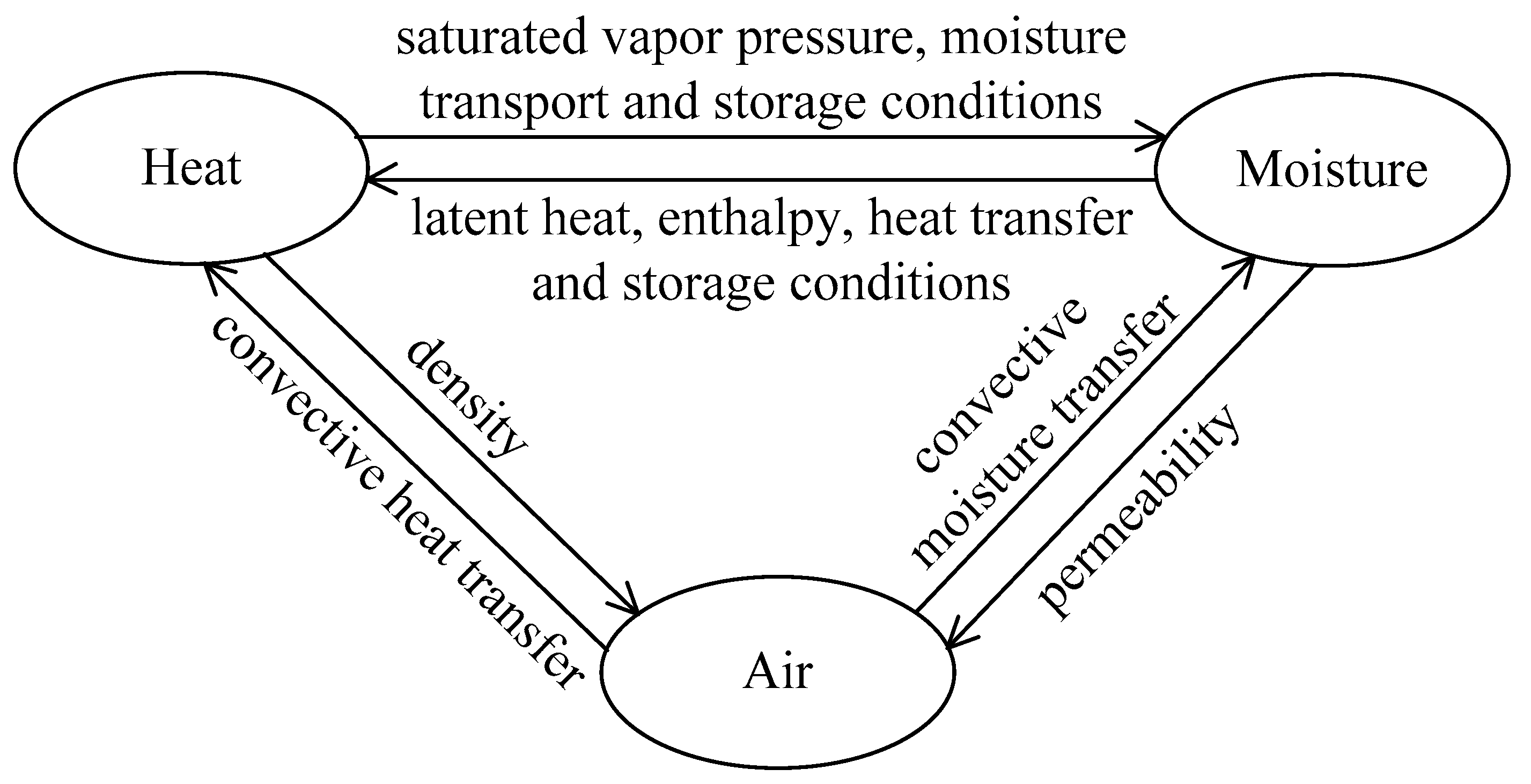
2.1. Numerical Simulation of Heat and Mass Transfer

The model geometry was 180 mm wide, 230 mm tall, 80 mm deep, and its envelope was 1.14 mm thick, exactly those of a real enclosure used in the library (Figure 1). The laminar airflow was assumed to align with the width of the enclosure, infiltrating through both the envelope and the gas of the enclosure. The air can flow through the gaps to the free-flow domain inside the empty enclosure and also permeate the porous domain of the cardboard.

In the storage room, the airflow velocity of supply air was approximately 0.2 m/s (the Reynolds number = ${\displaystyle \frac{\rho vl}{\mu }}={\displaystyle \frac{1.2\times 0.2\times 0.002}{1.8\times {10}^{-5}}}=26<2000$ laminar flow), and the temperature was between 15 and 25 °C. The airflow was expected to affect the convective heat and mass transfer, which consequently led to phase change and water vapor diffusion in the cardboard material. This hygrothermal response of the material was a key point to understanding the buffering effect on mitigating the hygrothermal fluctuation in the micro-environment inside the enclosure. The enclosure envelope could retain and release heat and moisture, and its hygrothermal condition was influenced by the conditions in both the micro- and macro-environments. Meanwhile, the hygrothermal conditions of both the micro- and macro-environments were interacting with each other through both the porous material and the gap. Hence, a two-way coupling was necessary in this study for the two-fold interaction with the two hygrothermal variables.

Figure 2 shows the interdependence of heat and moist-air transfer. The heat and moisture balance are coupled in a way that the latent heat, moisture state, transfer characteristic, and thermal storage affect the heat transfer, while the heat transfer determines the saturated vapor pressure, moisture driving force, and storage conditions. The heat and moist-air convection balance are coupled in a way that the temperature affects the air density, and conversely, the air convective heat transfer affects the temperature field. The moisture and air convection balance are coupled in a way that the airflow determines the convective moisture transfer, and in turn the vapor permeability determines the airflow in the porous media. To consider the complexity of modeling, we selected the direct coupling method, regarding the water vapor and air as one fluid in both the free-flow domain and porous domain. The space of these two domains is continuous, and a single set of conservation equations is solved by one solver in the simulation [22].

The Equations (1)–(3) show the mathematical description [23,24]:

$${\left(\rho C_p\right)}_{eff}{\displaystyle \frac{\partial T}{\partial t}}+\rho C_{p}u·\nabla T-\nabla ·\left(k_{eff}\nabla T+L_V{\delta }_P\nabla \left(\varphi p_{sat}\right)\right)=Q$$

(1)

$$\xi {\displaystyle \frac{\partial \varphi }{\partial t}}+\rho u\nabla {\omega }_v-\nabla ·\left(\xi D_W\nabla \varphi +{\delta }_P\nabla \left(\varphi p_{sat}\right)\right)=G$$

(2)

$$\rho \left({\displaystyle \frac{\partial u}{\partial t}}+u·\nabla u\right)+\nabla ·(pI-K)=F$$

(3)

where ${\left(\rho C_p\right)}_{eff}$ is the effective volumetric heat capacity at constant pressure, $\rho$ is moisture air density [kg/ m³], $C_p$ is heat capacity [J/(kg·K)]. $u$ is moisture air velocity [m/s]. $T$ is the temperature [K]. $k_{eff}$ is the effective thermal conductivity [W/(m·K)]. $L_V$ is the latent heat of evaporation [J/kg]. ${\delta }_P$ is vapor permeability [s]. $\varphi$ is the relative humidity. ${\omega }_v$ is vapor mass fraction. $p_{sat}$ is the vapor saturation pressure [Pa]. $Q$ is the heat source [W/m³·s]. $\xi$ is the moisture storage capacity [kg/ m³], $\xi ={\displaystyle \frac{\partial w\left({\varphi }_w\right)}{\partial {\varphi }_w}}$. $D_W$ is the moisture diffusivity [m²/s]. $G$ is the moisture source [kg/m³·s]. $p$ is the fluid pressure [N/m²]. $I$ is the identity tensor. $K$ is the viscous force [N/m²]. $F$ is the external force applied to the fluid [N/m²].

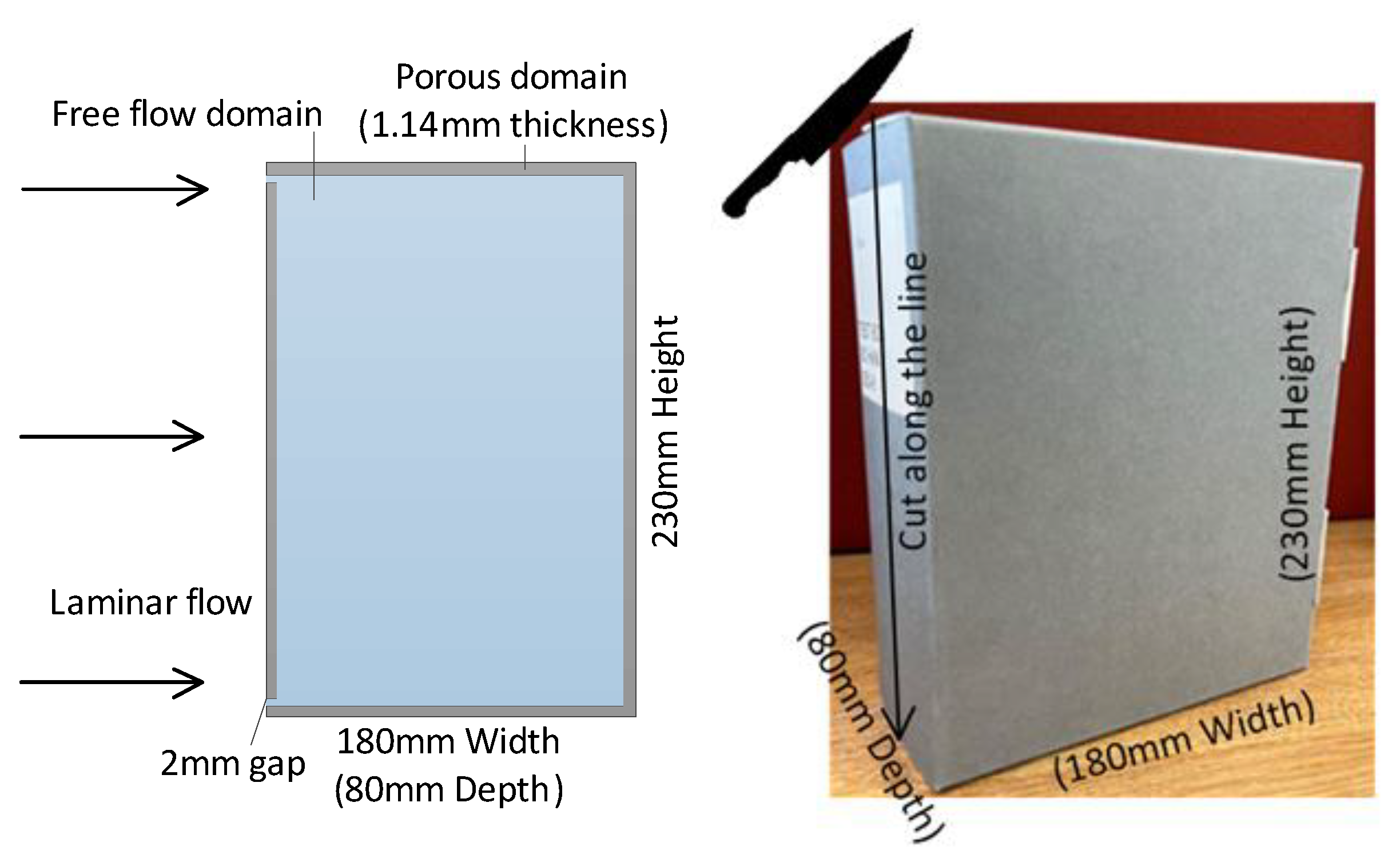
2.1.1. Model Setting

Because of limited computing resources in transient heat and mass simulation, a 2D axial-symmetry model with depth was used to represent the 3D model. The heat and mass model were developed in COMSOL Multiphysics 5.2 Win. Associated settings include four parts, (1) material setting, (2) boundary and initial conditions, (3) building mesh for the model, (4) solver setting, as

Table 1. Model setting.

Description	Value	Unit
① Carboard material
Density	662	kg/m3
Thermal conductivity	0.055	W/(m·K)
Heat capacity at constant pressure	1.028	J/(kg·K)
Diffusion coefficient	1.49 × 10−10	m2/s
Water content	$W_c=\rho \left(0.1237\times RH+0.0034\right)/1000$	kg/m3
Vapor resistance factor	95.63	-
② Boundary condition
Laminar air flow	0.2	m/s
Temperature	macro-environmental temperature	°C
RH	macro-environmental RH	%RH
Upper and lower gaps of the enclosure	open boundary	-
Initial conditions
Temperature and RH in both domains	macro-environmental temperature and RH at the first second	°C and %RH
Velocity in both domains	0.2	m/s
Pressure in both domains	(ambient pressure—reference pressure)	Pa
③ Meshing
Element types	triangular or quadrilateral	-
No. of layers in porous media	2~4	-
Mesh density	dense in the porous domain and gradually course toward the center of free flow domain	-
Maximum element growth rate	1.05	-
Maximum curvature factor	0.2	-
④ Solver
Time stepping	second-order BDF	-
Maximum step	0.25	h
Solving method	automatic Newton	-
tolerance factor	0.01	-
maximum No. of iterations	4	-

shows.

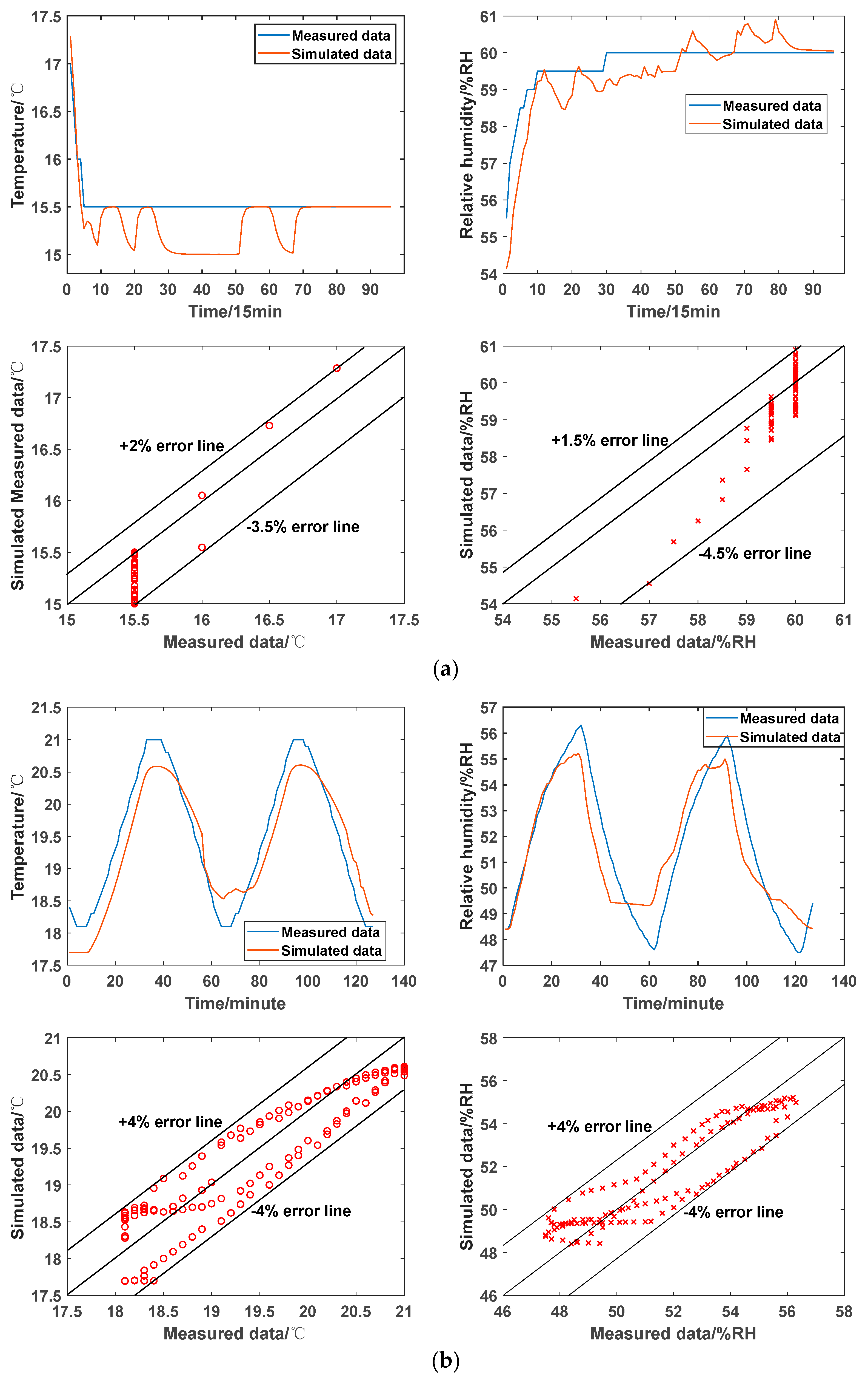
2.1.2. Model Validation

To meet the library’s preventive conservation requirements, the macro-environment must be strictly maintained at 15–25 °C and 40–60 %RH. Within these bands, different macro-environmental fluctuations affect the interaction of heat and mass transfer, especially for the hygrothermal response from the porous media of the cardboard. Therefore, the measurement data used for model validation should encompass different degrees of these fluctuations.

Three sets of micro-environmental data were gathered under varying levels of macro-environmental control accuracy. The first set originated from the library’s storage room, where tight control was maintained. The second and third sets were obtained in a controlled test chamber, where fluctuations of 10 %RH (ranging from 50 to 60 %RH) and 5 °C (fluctuating between 17 °C and 22 °C) occurred cyclically every 60 min. In each case, fixed conditions of 20 °C and 50 %RH were maintained, respectively.

The temperature and RH in the center of the free-flow domain were selected as simulated data to compare with the measured data. The maximum absolute and relative errors were used to evaluate the model accuracy [25].

$$\left\{\begin{array}{c}Max.absoluteerror=max\left\{{|{TorRH}_{measurement}-{TorRH}_{simulated}|}_t\}\right.\\ Maxrelativeerror=\max \left\{{{\displaystyle \frac{\left({TorRH}_{measurement}-{TorRH}_{simulated}\right)}{{TorRH}_{measurement}}}}_t\right\}\end{array}\right.$$

(4)

where $t$ is the sampling time for each 15 min in measurement and simulation.

Additionally, agreement between measurement and simulated data was indicated by Kling-Gupta Efficiency (KGE). It is given as Equation (5) [26].

$$\mathrm{K}\mathrm{G}\mathrm{E}=1-\sqrt{{(r-1)}^2+{(\beta -1)}^2+{(\alpha -1)}^2}$$

(5)

where $\beta ={\displaystyle \frac{{\mu }_s}{{\mu }_o}}$, ${\mu }_s$, and ${\mu }_o$ are means of the simulated and measurement data with time series; $\alpha ={\displaystyle \frac{{\sigma }_s}{{\sigma }_o}}$, ${\sigma }_s$, and ${\sigma }_o$ are standard deviations of the simulated and measurement data with time series.

Negative KGE values are regarded as bad model performance, while the positive values show a good performance. KGE = 1 indicates perfect agreement in terms of correlation, mean, and variability. KGE > 0.5 indicates that a model’s performance is above the baseline in empirical terms [27].

2.2. Determination of Acceptable Macro-Environment

Relaxing the tight macro-environment on the site is impractical due to strict regulations of management in the storage room. Therefore, it is necessary to amplify the macro-environmental fluctuations based on the HAM simulation. The three-stage method of data acquisition was developed to generate data and further determine an acceptable macro-environment. It included macro-environmental data amplification, heat and mass simulation, and acceptable macro-environment determination (Figure 3). Stage 1 was about macro-environment data acquisition. In Stages 2 and 3, there was a loop to search the upper limit of the acceptable macro-environment by using the trial-and-error method.

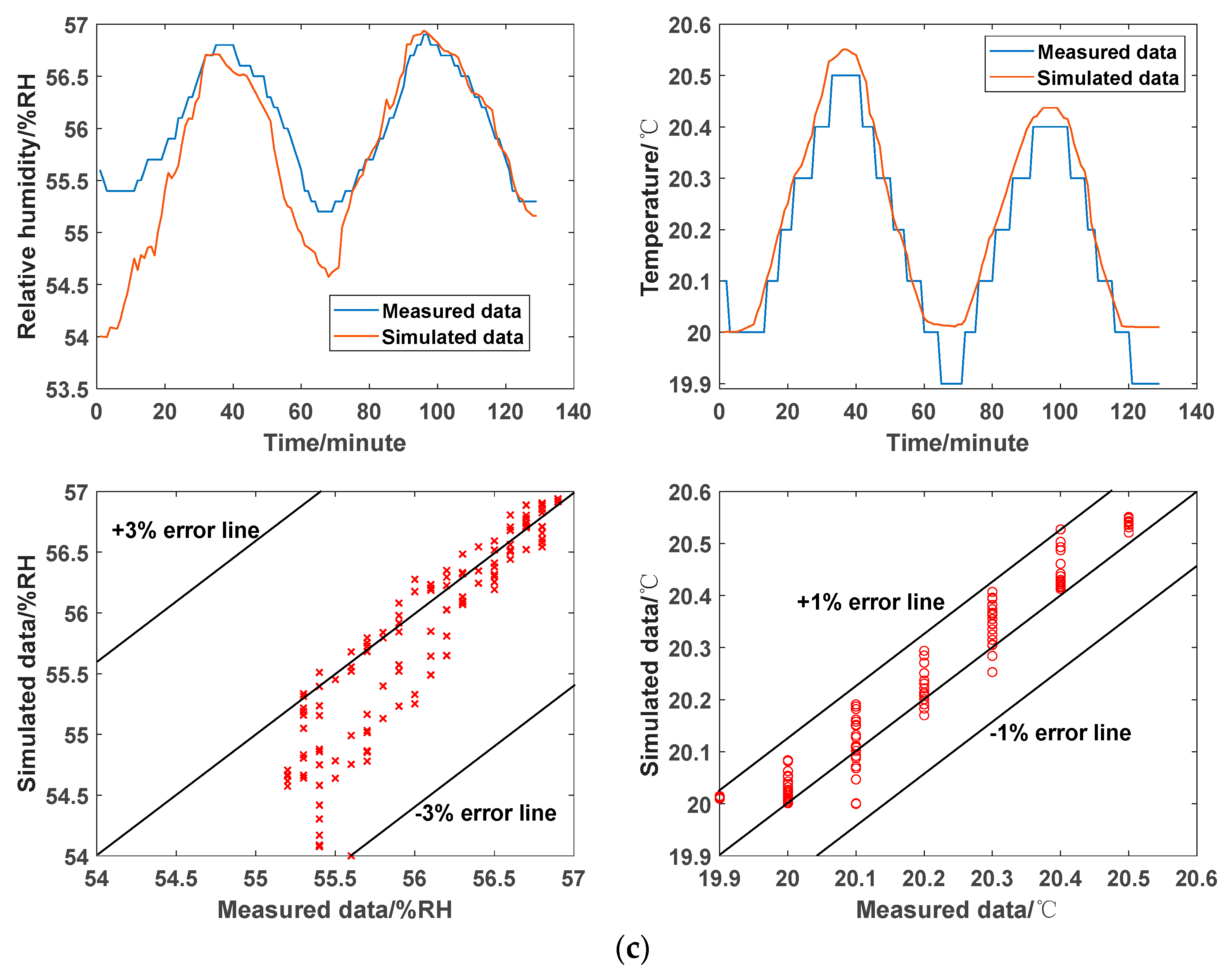
2.2.1. Typical Reference Data Selection

The choice of typical reference (TR) data was intended to identify four representative weeks of data, each encapsulating the distinct characteristics of the four seasons within a two-year dataset collected from the storage room. The typical-meteorological-year (TMY) data generation method in building energy simulation was used [28]. It was based on the Finkelstein–Schafer (FS) statistical method [29]. Each week was selected within a specific season in these two years. The daily means of macro-environmental temperature and RH were calculated. Then, they were sorted into an ascending order to calculate the cumulative distribution function (Equation (6)) for each week ($F_{n,w}\left(x\right)$) in the long term and individual season of that week ($F_{n,w,s}\left(x\right)$) in the short term.

$$F_n\left(x\right)=\left\{\begin{array}{c}0,x<x_1\\ \left(k-0.1\right),x_k\le x\le x_{k+1}\\ 1,x>x_n\end{array}\right.$$

(6)

where $x$ is the daily mean of temperature or RH, $k$ is the rank order, $n$ is the number of $x$.

The FS statistic was calculated by Equation (7).

$$FS\left(s,w\right)={\sum }_{k=1}^n|F_{n,w,s}\left(x_k\right)-F_{n,w}\left(x_k\right)|$$

(7)

where $F_{n,w,s}\left(x_k\right)$ was calculated by the daily means within that week and that season. $F_{n,w}\left(x_k\right)$ was calculated by the daily means over these two years. The typical week for each season was determined by that week that has the smallest $FS\left(s,w\right)$.

The typical reference data was amplified to obtain new data reflecting the macro-environment in the relaxing control.

2.2.2. Data Amplification

The principle of data amplification drew inspiration from electroencephalogram (EEG) signal processing. The EEG signal can be regarded as a time-dependent amplitude function that is expressed as a spectrum in different frequencies [30,31]. It was associated with five typical brain activities, including relaxed awareness without any attention (alpha waves), active thinking (beta waves), deep sleep (delta waves), deep meditation (theta waves), and some certain brain diseases (gamma waves) [32]. An analogy was made between the EEG signal processing and the macro-environment data processing. The data can be decomposed into many components to represent the data features. Each key feature can be regarded as a factor that affects the macro-environmental fluctuations. The Fourier transform (FT) is a tool to achieve data transformation between the time domain (original data) and the frequency domain (features). It can be expressed by Equation (8) [33].

$$X\left(k\right)={\sum }_{j=1}^{n}x\left(j\right)W_n^{(j-1)(k-1)}$$

(8)

And the inverse FT can be expressed by Equation (9).

$$x\left(j\right)={\displaystyle \frac{1}{n}}{\sum }_{k=1}^{n}X\left(k\right)W_n^{-(j-1)(k-1)}$$

(9)

where $X\left(k\right)$ and $x\left(j\right)$ are the FT pairs in time and frequency domains. $X\left(k\right)$ is the macro-environmental data with $k$ points sequence. $x\left(j\right)$ can be regarded as $j$ data features with successive amplitude at specific frequencies. $W_n=e^{(-2\pi i)/n}$ is a primitive n-th root of 1. $i=\sqrt{-1}$, the imaginary unit.

The daily RH data, $X\left(k\right)$, was decomposed to the data features, $x\left(j\right)$, by using the FT function tool in MATLAB 2024a Win. A subset of key frequency components was intentionally selected to represent the key features of the original data. Once the set of key features was determined, the decomposition process became repeatable. These components were combined by using the inverse FT to reconstruct an approximate version of the original data. The accuracy of this reconstruction depended on the number of selected components. The selection threshold was set at a high R-squared value, R² ≥ 0.95, between the original data and the represented data. Sequentially, the selected components $x\left(j\right)$ were scaled by an amplification factor and inversely transferred back to the time domain to obtain the data with large fluctuations. This synchronous amplification was based on the conservative assumption that all the selected components experienced maximum amplification simultaneously, representing a worst-case scenario for collection care.

The trial-and-error method was used to amplify the fluctuations gradually until the micro-environment did not comply with the specifications of preventive conservation in the risk assessment.

The data amplification of macro-environment applied to RH only, excluding temperature, has two reasons. First, as a useful approximation in RH control for preventive conservation, a coupled RH change of 3% occurs for each degree of temperature change [34]. A slight temperature change possibly could cause the RH out of the control band or allowable range of 24 h fluctuation. The setting of temperature change is dependent on the RH control requirement in the precision air conditioning with humidity priority because the RH change in paper-based collection storage directly impacts paper stability and preservation. Second, the thermal mass of the library’s storage room can ensure a small fluctuation for indoor temperature. Throughout the two-year dataset, the macro-environmental temperature remained consistently within the range of 17–20 °C, with fluctuations of ≤0.2 °C occurring for 95% of the time. The relaxation of temperature control was not considered.

2.2.3. Determination Process of Acceptable Macro-Environment

In preventive conservation, the micro-environmental data must comply with the specifications, 15~25 °C, 40~60 %RH control bands, and <±5 °C, <±10 %RH 24 h fluctuations for most paper-based collections. The risk assessment checked the micro-environmental temperature and RH, which were output from the heat and mass simulation.

A sliding window calculator was developed as Equation (10) shows; it helps to check the maximum and minimum values and the biggest fluctuation in any 24 h (96 sampling points). In this risk assessment, if the micro-environment complies with the specifications, the associated macro-environment can be accepted. The amplification factor was increased to amplify the macro-environmental fluctuations in the loop designed to search the upper limit of acceptable macro-environment.

$$\begin{array}{c}for i=1:n\hfill \\ \left\{\begin{array}{c}\max \left\{{RH}_i,\dots ,{RH}_{i+95}\right\}-\min \left\{{RH}_i,\dots ,{RH}_{i+95}\right\}\le 10\%\\ \max \left\{{\mathit{RH}}_i,\dots ,{\mathit{RH}}_{i+95}\right\}\le 60\%\\ \min \left\{{RH}_i,\dots ,{RH}_{i+95}\right\}\ge 40\%\end{array}\right.\end{array}$$

(10)

where $n$ is the number of sliding windows, $n$ = 2592 (4-week of data).

2.3. ANN Modeling

2.3.1. Data Preparation

Based on the above Section 2.2, within the range of acceptable macro-environment, four sets of data were prepared to represent four levels of macro-environmental control accuracy in the relaxing control (

Table 2. Four datasets in the relaxing control.

Level	24 h Fluctuation (Band) in Macro-Environment	24 h Fluctuation (Band) in Micro-Environment	Amplification Factor
1	±10 (42.2~56.1) %RH	±7.1 (45.5~55) %RH	10
2	±12 (39.6~57.4) %RH	±7.9 (44.7~55.4) %RH	11.6
3	±14 (37~59.4) %RH	±8.1 (43.8~56.8) %RH	13.4
4	±16 (33~65) %RH	±9.1 (43~57.3) %RH	15

).

These levels from 1 to 4 signify the control accuracy of macro-environment from the current control requirement level based on the specifications of preventive conservation to the most relaxing level determined in Section 2.2.3. These four generated datasets, along with the on-site collected dataset under tight control, denote varying levels of control accuracy within the acceptable conditions. They were used for ANN training. The macro-environmental temperature and RH were input, and the corresponding micro-environmental ones were output. To improve stability during the training, it requires a normalization process for all input and output data before the training [35]. An inverse normalization is necessary to predict the outputs after the training. Thus, Z-score normalization was used to rescale the data with zero mean and a unit variance here. The total dataset size is 10,752 with a 15 min interval. This time resolution aligns with a typical setting in the NLS. The time-series dataset was divided into two parts for training. Ninety percent of the data was allocated for the training process, and the rest of the ten percent was allocated for testing the trained networks to evaluate the prediction accuracy [36,37].

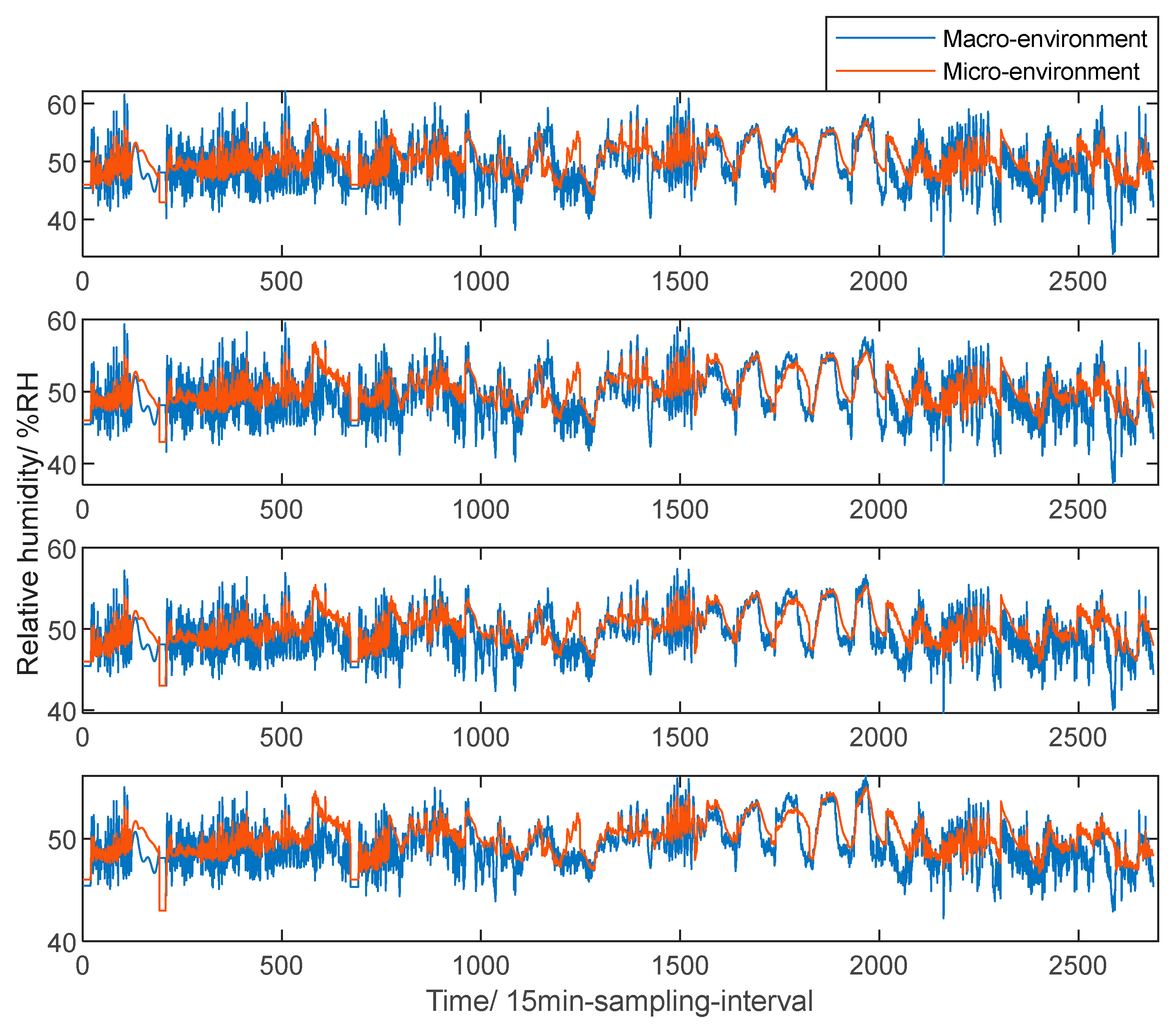
2.3.2. Architecture of the ANN

The real-time prediction of the micro-environment should consider the data relationship sequence-to-sequence, inputting 24 h macro-environmental temperature and RH to predict the corresponding micro-environmental ones. Long short-term memory (LSTM) network, a type of ANN, was designed to solve this problem [38] (Figure 4). The architecture consisted of a forget gate, input gate, and output gate to achieve appropriate-term memory. The mathematical expressions about the forget gate, input gate, output gate, and hidden layer are given by Equation (11) [39].

$$\left\{\begin{array}{c}{f}_t=\sigma \left(W_{fh}{h}_{t-1}+W_{fx}{x}_t+b_f\right)\\ i_t=\sigma \left(W_{ih}{h}_{t-1}+W_{ix}{x}_t+b_i\right)\\ {\tilde{c}}_t=\tanh \left(W_{\tilde{c}h}{h}_{t-1}+W_{\tilde{c}x}{x}_t+b_{\tilde{c}}\right)\\ c_t=f_t·c_{t-1}+i_t·{\tilde{c}}_t\\ o_t=\sigma \left(W_{oh}{h}_{t-1}+W_{ox}{x}_t+b_o\right)\\ h_t=o_t·\tanh \left(c_t\right)\\ y_t=h_t\end{array}\right.$$

(11)

where $f_t$ is the forget factor to decide on which information should be kept and which to forget. $\sigma$ and $tanh$ are sigmoid (the value is between 0 and 1) and hyperbolic tangent (the value is between −1 and 1) activation functions, respectively. $h_t$, $i_t$, ${\tilde{c}}_t$, $c_t$ and $o_t$ denote the recurrent information, input factor, candidate cell state, cell state and output factor. $W_f$, $W_i$, $W_{\tilde{c}}$ and $W_o$ are the weights, and $b_f$, $b_i$, $b_{\tilde{c}}$, and $b_o$ are the bias. $c_t$ denotes the cell state of the neural network. The operator ‘$·$’ denotes the pointwise multiplication of two vectors. $x_t$ and $y_t$ are the input and output.

The LSTM network uniquely captured sequence-to-sequence relationships between macro- and micro-environments, demanding deep learning for intelligent decision-making during training. Its architecture included specialized layers to leverage the intelligence of its three gate-operated memory units. Dropout was a regularization technique to prevent overfitting issues in the neural network. Setting a dropout layer between the hidden layers and the last hidden layer—the fully connected layer (also called the dense layer)—could effectively prevent this issue in RNN training [40,41]. Fully connected layers allowed the network to capture the dependence between various features by using non-linear transformations to the input data [42]. Because there was dependence between temperature and RH with a highly non-linear relationship, a fully connected layer could contribute to effective data mapping here. The regression layer was selected as the output layout because the data mapping between macro- and micro-environments was a many-to-many regression problem.

Therefore, the basic architecture of our LSTM should include a sequence input layer, LSTM layer(s), dropout layer(s), fully connected layer, and regression output layer (Figure 5). The optimal number of LSTM layers and associated neurons was determined by a trial-and-error method (Figure 6). We relied on past research on LSTM training to determine the maximum number of LSTM layers and neurons (5 and 250) for searching for the optimal architecture [43,44]. To assess the accuracy of the trained network, the latest RMSE and absolute errors of the trained network were compared with the errors from previous training in the loop and the measurement errors (±0.5 °C and ±3 %RH in the library’s storage room), respectively. If they are smaller than both the earlier prediction errors and the measurement errors, it means that this trained network has minimal prediction errors and acceptable accuracy. Otherwise, the numbers of layers and neurons should be increased gradually until the best architecture is found.

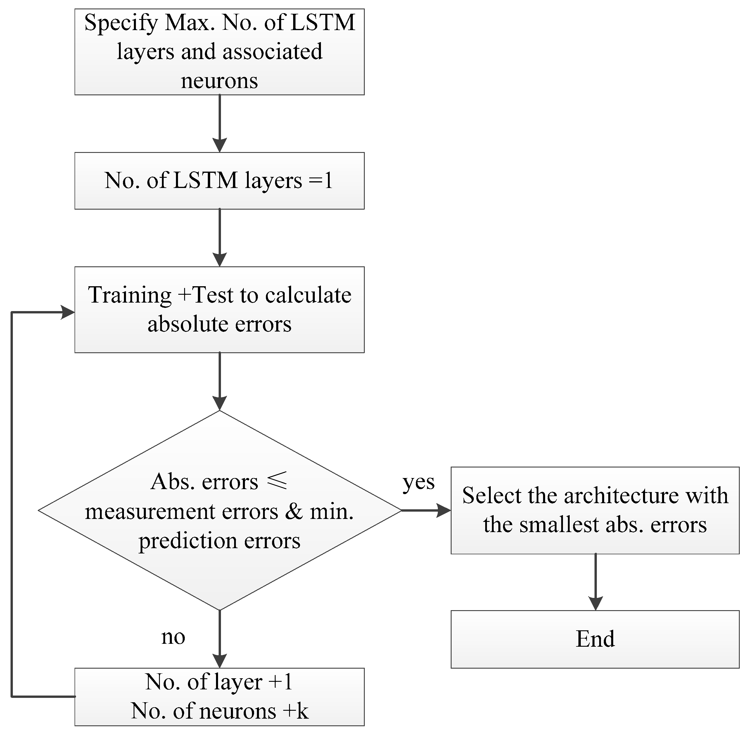
2.3.3. Evaluation of the Optimal LSTM Network

An evaluation of the network was conducted in the training set and testing set, respectively. The overfitting problem happens when there is an extremely high accuracy in the training set but a low accuracy in the testing set. Oppositely, the underfitting problem happened when both accuracies were low, but the testing one was higher than the training one [45,46]. Their accuracies were assessed to guarantee that the model at the sweet spot was between underfitting and overfitting, which ensures a good generalization performance.

Statistical criteria were used to evaluate the accuracy of the LSTM network [47]: coefficient of determination ($R^2$), mean square error ($MSE$), root mean square error ($RMSE$), mean absolute error ($MAE$), and standard deviation of the errors (StD of errors). These evaluation indicators were defined mathematically as follows:

$$R^2=1-{\displaystyle \frac{{\sum }_{i=1}^m{(y_{i\left(actual\right)}-{\widehat{y}}_{i\left(predicted\right)})}^2}{{\sum }_{i=1}^m{(y_{i\left(actual\right)}-{\overline{y}}_{i\left(actual\right)})}^2}}$$

$$MSE={\displaystyle \frac{1}{m}}{\sum }_{i=1}^m{(y_{i\left(actual\right)}-y_{i\left(predicted\right)})}^2$$

$$RMSE=\sqrt[2]{{\displaystyle \frac{1}{m}}{\sum }_{i=1}^m{(y_{i\left(actual\right)}-y_{i\left(predicted\right)})}^2}$$

$$MAE={\displaystyle \frac{1}{m}}{\sum }_{i=1}^m\left|y_{i\left(actual\right)}-y_{i\left(predicted\right)}\right|$$

$$StD of errors=\sqrt[2]{{\displaystyle \frac{1}{(m-1)}}{\sum }_{i=1}^m{(E_{i\left(predicted\right)}-{\overline{E}}_{i\left(predicted\right)})}^2}$$

where $y_{\left(actual\right)}$ and $y_{\left(predicted\right)}$ are actual value and the predicted value, $m$ is the number of data, and $E$ is the error between the actual value and predicted value.

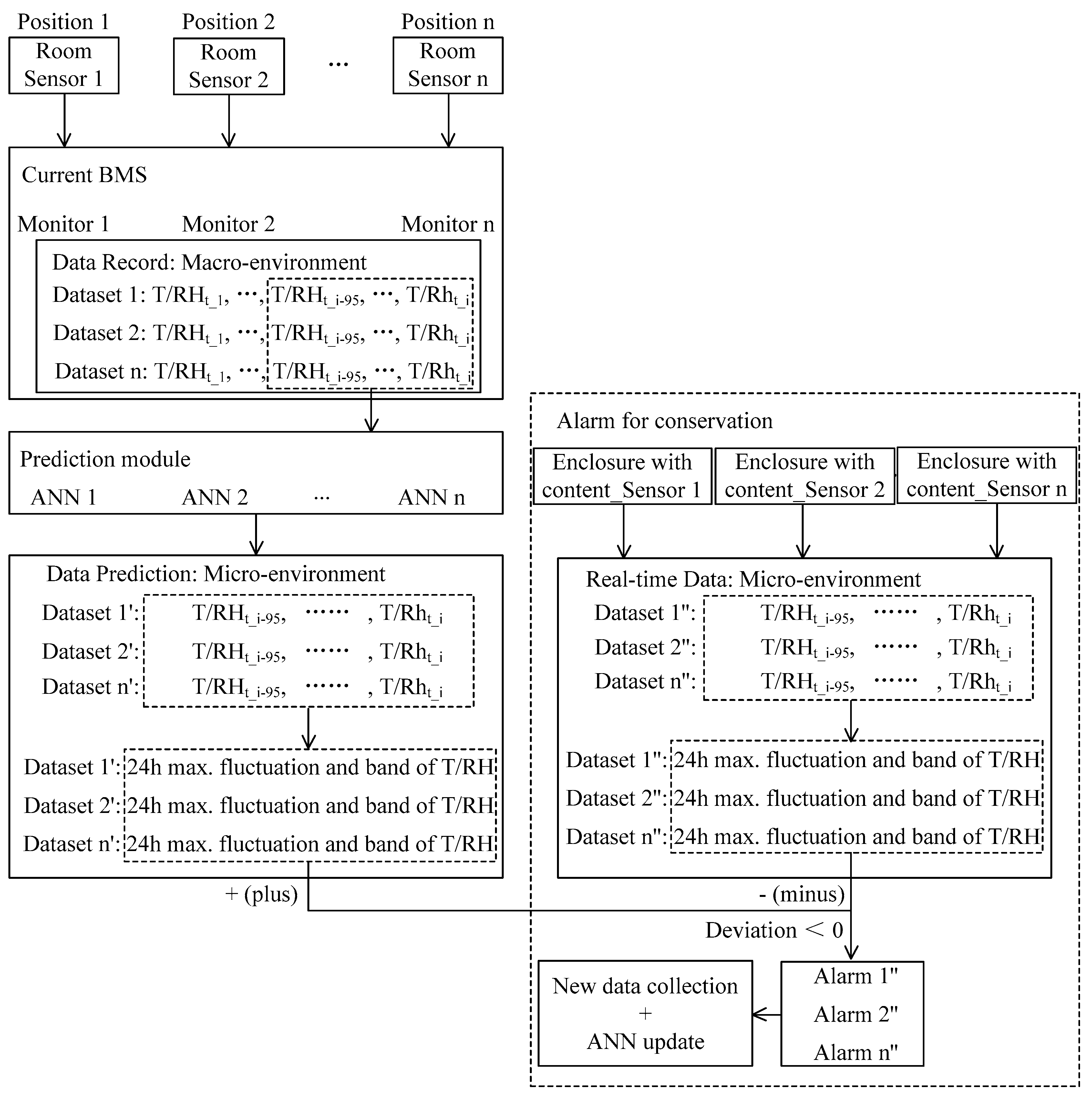
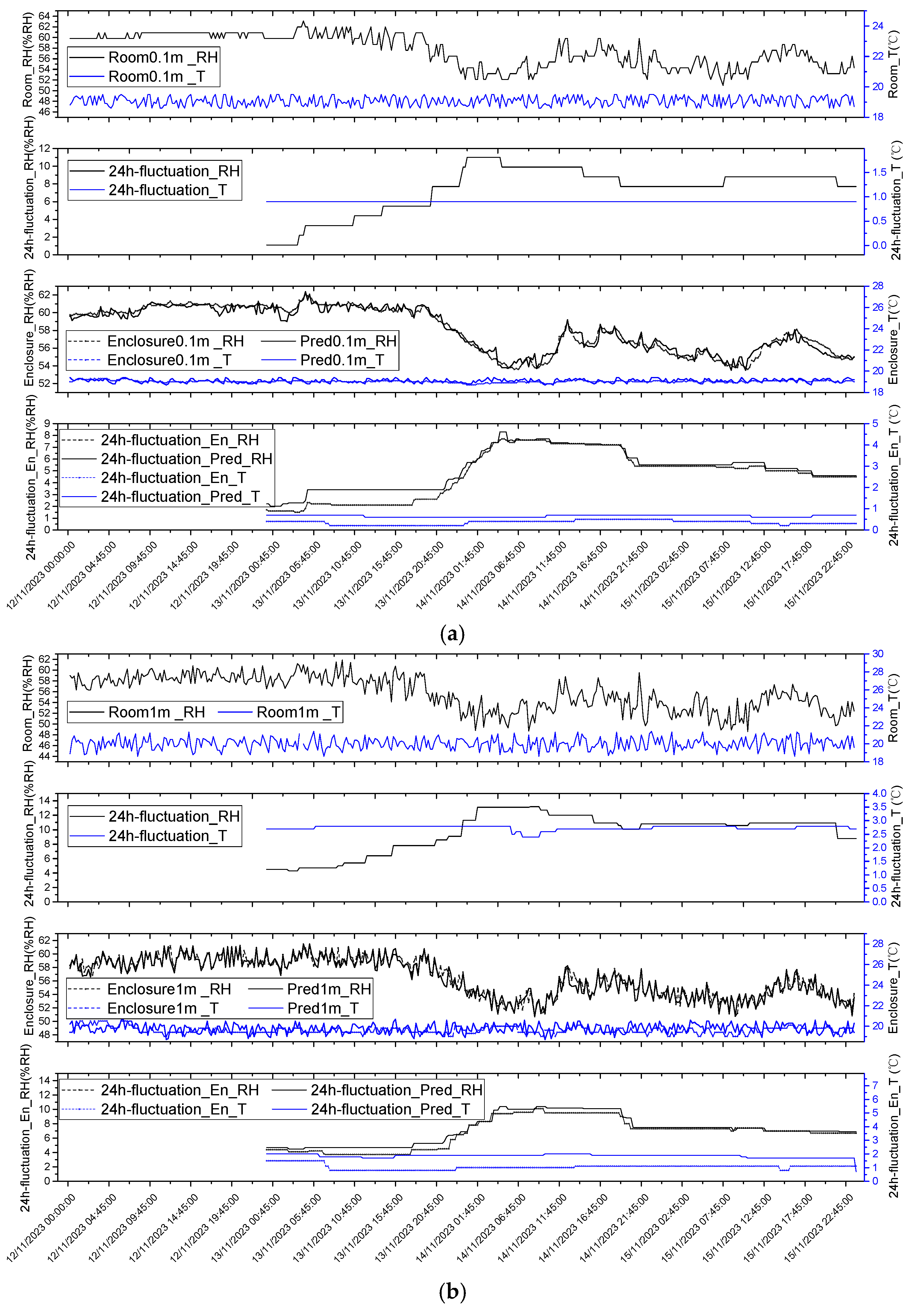
2.3.4. Practical Application of Real-Time Conformity Monitoring

The evaluation of the ANN model demonstrates the accuracy of micro-environmental prediction for the empty enclosure, which represents the worst-case scenario for hygrothermal buffering compared to enclosures containing paper-based collections. However, assessing the performance of the ANN model in practical applications is essential. This part of the study aims to assess the robustness of real-time prediction for monitoring micro-environmental conformity in practical scenarios where enclosures with paper-based collections are used.

Validation Experiment

The trial was carried out in a test room, 5 m long, 3 m wide, and 3 m tall (Figure 7). Inside the room, the air distribution was created to match that of the library’s air-conditioning configuration, with air supplied from the top and returned from the bottom, setting the velocity of supply air at approximately 0.2 m/s to prevent dust buoyancy. The macro-environment was controlled to fall within the range of 16~32 °C and 30~80 %RH, with an accuracy of approximate ±2 °C and ±10 %RH. The operational points were set at 20 °C and 55 %RH for this trial. These conditions represent the common NLS operating environment, which exhibits minimal seasonal variation.

The trial was carried out in a controlled chamber 5 m long, 3 m wide, and 3 m tall (Figure 7). Inside this room, the conditioned air went into the room space through a void above a grid ceiling and then returned at a low level through three vents 0.1 m above the floor. The desk panel was meant to separate two airflow zones. The upper zone was inside the mainstream, while the lower one experienced more turbulence. These configuration efforts were to replicate the air distribution of the real scenario for validation purposes.

Two enclosures were strategically placed in the two zones to account for temperature and humidity fluctuations across varying spatial gradients inside the space. They were filled with 70% full newspapers to represent the most common use of these enclosures. Additionally, two temperature and humidity loggers (loggers 2 and 4 in Figure 7) were placed inside these enclosures to record the micro-environment conditions. Another two loggers (loggers 1 and 3 in Figure 7) were positioned near these enclosures to monitor the macro-environment. Their measurement accuracies are ±1 °C (within the range of 5–60 °C) and ±3 %RH (within the range of 20–80 %RH). The sampling interval for all loggers was set at 15 min, consistent with the interval used in the BMS (Building Management System).

Parallel Prediction

To predict the micro-environment within various enclosures positioned differently, we replicated the trained ANN for each of the sensors located in the macro-environment. The trained ANN models were to act as parallel predictors in a BMS (Figure 8). The ANNs were fed with the latest 24 h macro-environmental data, consisting of 96 data points with 15 min sampling intervals from the on-site monitoring, to predict the micro-environmental condition.

The maximum fluctuations and associated bands in the predicted results were calculated. Simultaneously, a real-time measurement of micro-environment was conducted to assess the prediction in the trial test. Analyzing environmental data helps identify risks specific to the collections with various materials, but this inherent diversity makes this process complex [48]. Therefore, the ANN prediction was based on the worst-case scenario or the least buffering effect, an empty box with no collections inside to further moderate the micro-environmental fluctuations. This resulted in larger predicted fluctuations and bands compared to real-time measurements, which understandably led to deviations between the predicted and measured data. These deviations are defined as follows:

(1) ${24 \mathrm{h} \mathrm{F}\mathrm{l}\mathrm{u}\mathrm{c}\mathrm{t}\mathrm{u}\mathrm{a}\mathrm{t}\mathrm{i}\mathrm{o}\mathrm{n}}_{prediction}-{24 \mathrm{h} \mathrm{F}\mathrm{l}\mathrm{u}\mathrm{c}\mathrm{t}\mathrm{u}\mathrm{a}\mathrm{t}\mathrm{i}\mathrm{o}\mathrm{n}}_{measurement}$

(2) ${{\mathrm{T}/\mathrm{R}\mathrm{H} \mathrm{b}\mathrm{a}\mathrm{n}\mathrm{d}}_{measurement}\in \mathrm{T}/\mathrm{R}\mathrm{H} \mathrm{b}\mathrm{a}\mathrm{n}\mathrm{d}}_{prediction}$ (the measurement bands are included in the prediction control ones).

These deviations provide a critical region between safe and dangerous conditions for preventive conservation. A positive value indicates that the actual micro-environment is more stable and safer than the predicted condition. Conversely, a negative value indicates that there is no critical region, and the actual conditions fall outside the scenarios captured by the trained ANN predictor, which triggers a built-in alarm. In such conditions, retraining the ANN with new measurement data is necessary.

The test was run continuously for four days to assess the robustness of these ANN predictors working in real-time. If any alarms are triggered during the test, that ANN model should be retrained with new data to improve its robustness. Conversely, if no alarm was triggered, the robustness could be considered acceptable.

3. Results and Discussion

3.1. Comparison of Measured and Simulated Data in Heat and Mass Simulation

Comparison between the measured data and the simulated data for micro-environment temperature and RH shows relative errors within ±4% for temperature and ±4.5% for RH, and absolute errors below 0.7 °C for temperature and 2.5% for RH (Figure 9). In detail, the accuracy of the simulation is demonstrated through a series of comparative figures. The first figure (a) illustrates the data for the tight control condition, where the errors are kept below 3.5% for temperature and 4.5% for RH. The subsequent figures present the conditions under more relaxed control. The second figure (b) depicts a scenario with a 5 °C fluctuation over a 60-min period at a fixed 50 %RH, where the relative errors are under 4% for both temperature and RH. The third figure (c) represents a 10% RH fluctuation over a 60-min period at a fixed 20 °C, with errors below 3% for temperature and 1% for RH. These results indicate the high accuracy of the simulation, validating its effectiveness in replicating real-world conditions.

To assess the agreement between measured and simulated data,

Table 3. KGE values for micro-environmental temperature and RH.

	Tigh-Control	↑↓5 °C @50 %RH	↑↓10 %RH @20 °C
KGE for temp.	0.51	0.84	0.97
KGE for RH	0.58	0.77	0.63

shows the KGE values in these three validation conditions. All values exceed the baseline (KGE ≥ 0.5), which indicates an acceptable agreement in simulating the heat, air, and moisture transfer between the micro-environment and macro-environment. The model effectively reproduces the variation trends and fluctuation periods in the measurement conditions for a subsequent study about the determination of an acceptable macro-environment.

However, the results show relatively high values in the last two measurement conditions with the relaxing control compared to the first condition with tight control. This suggests that the model exhibits greater agreement in the relaxing control than in the tight control.

3.2. Acceptable Macro-Environment

The upper limit of acceptable macro-environmental conditions was determined using the trial-and-error method within the searching loop. The macro-environment can be relaxed to an upper limit of 33–65 %RH with a ±16 %RH fluctuation over 24 h, while the current requirement is 40–60 %RH with a ±10 %RH fluctuation.

Correspondingly, the micro-environment RH can be maintained within the range of 43–57.3 %RH, with 24-h fluctuation of <±9.1 %RH, as shown in Figure 10. These results illustrate that the buffering capacity of the enclosure ensures a stable micro-environment with low RH fluctuation amplitude. This stability opens up the potential to relax current tight control in the macro-environment without any detrimental effect on the collections.

While only a single amplification loop was used, the assumption of data amplification across key frequency components serves as the worst-case scenario, thereby offering a conservative estimate of risk. In real-world applications, environmental fluctuations are typically less severe and less synchronized. Therefore, if the enclosure system proves effective under such amplified conditions, its performance under actual, more moderate variability can be considered robust. Nonetheless, future work should examine the sensitivity of this threshold under stochastic noise or uncertainties in the input data to further validate statistical robustness.

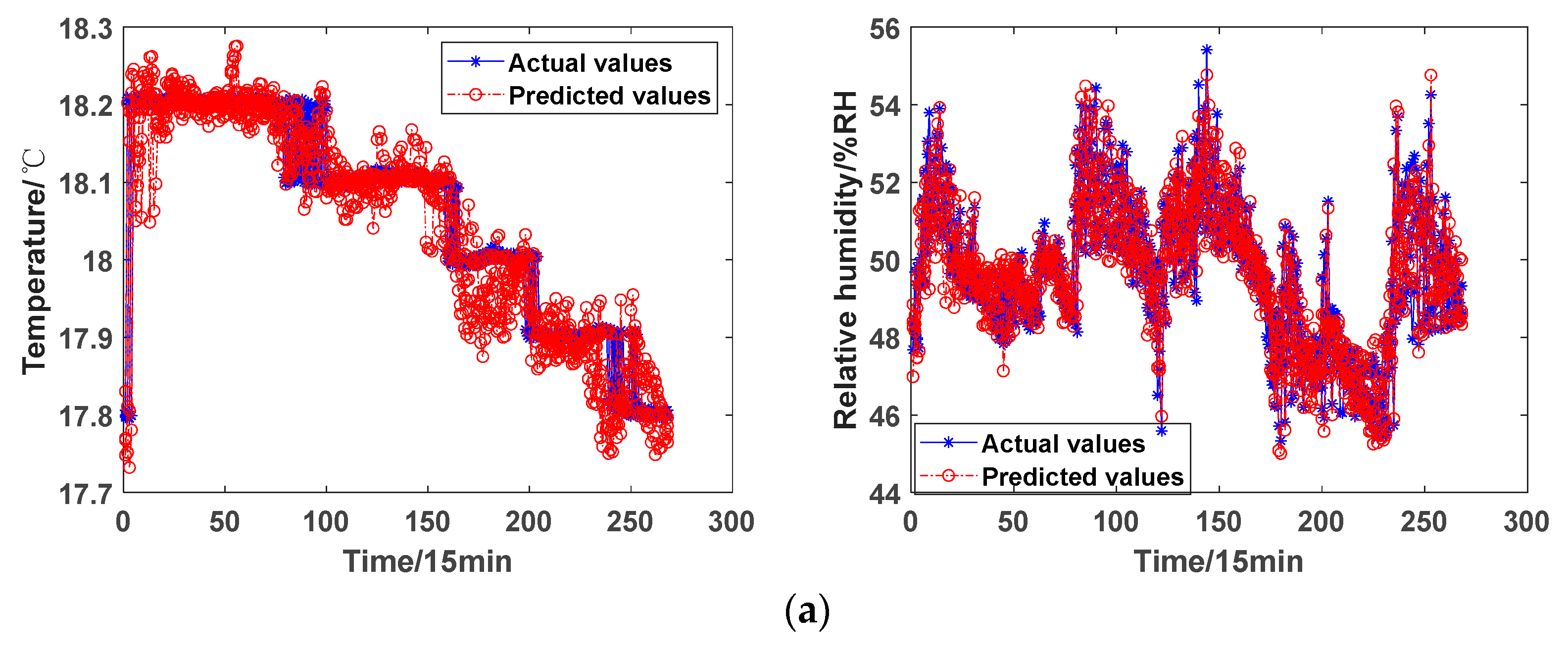
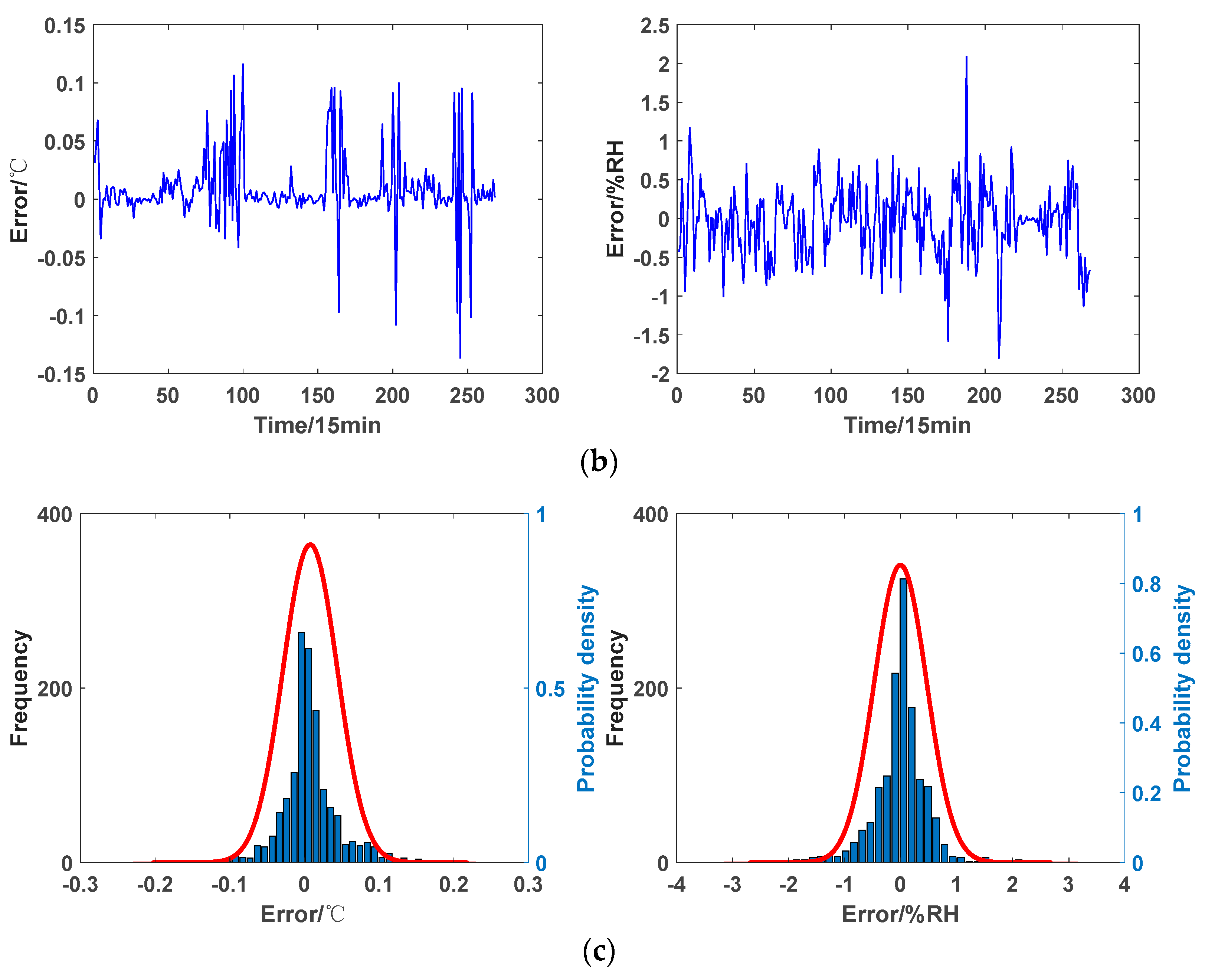
3.3. Real-Time Prediction of Micro-Environment

For data acquisition, four sets of data were generated to represent different levels of macro-environmental control accuracy, from ±10 %RH 24 h fluctuation to the most relaxing condition. They were prepared to illustrate the four levels of relaxing control within the acceptable macro-environment range, as shown in Figure 11. From the perspective of data expression, these datasets and the on-site dataset can reflect characteristics about the interaction of heat and mass transfer between macro- and micro-environments within the acceptable range.

For searching the optimal architecture, multiple LSTM networks were trained through a gradual increase in the number of hidden layers and neurons. The resulting RMSE and absolute errors are detailed in Figure 12. The RMSE values range from 0.037 to 0.188 for temperature and 0.467–1.73 for RH. Correspondingly, absolute errors vary from |−0.13| to 0.64 °C for temperature and |−8.2%| to 6.3% for RH.

The architecture with 2 layers demonstrates relatively high accuracy in prediction, while a single-layer configuration shows relatively low accuracy in RH prediction. As the number of layers increases from 1 to 4 in the networks with an equal number of neurons per layer, accuracy typically improves. However, as the number of neurons increases in the networks with an equal number of layers, beyond a certain threshold where the number of neurons exceeds a maximum, further increasing the number of neurons per layer can lead to a decline in accuracy. Both a relatively shallow LSTM network with many neurons and a deeper network with fewer neurons demonstrate strong performance.

In detail, for the 2-layer networks, the configuration with 200 neurons in each layer stands out as the most accurate. Comparing its absolute errors with measurement errors (±0.5 °C and ±3 %RH), it is noted that the absolute errors ranging from −0.13 to 0.15 °C and −2.2 to 2.2 %RH are smaller than the measurement errors. This suggests that the network can predict micro-environmental temperature and RH as accurately as on-site measurements.

Based on these findings, we conclude that the optimal LSTM network architecture consists of 2 layers, with each layer comprising 200 neurons. The selected architecture was found to balance prediction accuracy with computational efficiency. Beyond this configuration, additional neurons or layers increased training time significantly without noticeable accuracy improvement. In contrast, shallower networks showed reduced RH prediction accuracy, particularly under larger fluctuation conditions. The final model achieved a fast prediction time for 24 h of data on a standard CPU, suitable for real-time deployment.

Table 4. Performance results of the LSTM network.

	R2	RMSE	MSE	MAE	StD
Training data (temperature)	0.999	0.035	0.001	0.023	0.035
Training data (RH)	0.984	0.364	0.132	0.230	0.364
Testing data (temperature)	0.965	0.037	0.001	0.025	0.037
Testing data (RH)	0.963	0.468	0.219	0.313	0.468

shows the performance results of the optimal LSTM network. All coefficients of determination are close to 1, while the values of MSE, RMSE, MAE and StD are near 0. In addition, Figure 13 and Figure 14 illustrate: (1) the time-series prediction adeptly captures the fluctuation trends with accurate periods in both training and testing sets; (2) the absolute errors predominantly remain below ±0.2 °C and ±3 %RH in the training set, and ±0.1 °C and ±2 %RH in the testing set; (3) the error histograms present a distribution centered around zero with minimal deviation. These indicators indicate high accuracy in both training and testing processes. They affirm that this optimal network has robust generalization and accurate prediction performance without underfitting and overfitting problems. However, the current model is trained on a finite dataset that may not capture the full range of conditions experienced at the National Library of Scotland. To enhance generalizability and long-term reliability, future work will focus on incrementally incorporating additional real-world measurement data into the training process to further improve the ANN model’s robustness.

Additionally, the prediction time for daily data, comprising 96 data points, was less than 5 s by using a 1.6 GHz CPU with 16 GB RAM. Based on this trained LSTM network, any 24 h time-sequence macro-environmental temperature and RH data can be input to predict the corresponding micro-environmental ones inside the storage enclosure.

The model evaluation above indicated the accuracy of micro-environmental prediction under the worst-case scenario without any buffering effect from paper-based collections. The following results focus on assessing the model’s robustness in practical applications involving enclosures with collections inside.

Figure 15 shows data comparison between onsite measurement and ANN prediction. Notably, the micro-environment in the return air zone exhibits better stability compared to that in the supply air zone. Associated absolute errors are ±0.6 °C & ±1.6 %RH for the return air zone and ±0.9 °C & ±3 %RH for the supply air zone. These prediction accuracies are smaller than the onsite monitoring accuracy of ±1 °C and ±3 %RH, which is deemed acceptable for the real-time micro-environment prediction.

In addition, the temperature and humidity fluctuations in the return air zone range from 0.75 to 1 °C and 1 to 11 %RH, while the supply air zone has fluctuations of 2.5 to 3 °C and 4 to 13 %RH. Despite the larger fluctuations in the supply air zone, deviations of both zones are negative values with the critical region of approximately 0.3 °C and 1 %RH. It means that the measurement temperature and RH bands are encompassed within the prediction ones for any 24 h period, thus triggering no alarms.

This real-time prediction provides a feasible way to monitor the micro-environment, and to map the hygrothermal condition over multiple enclosures in the macro-environment, the storage room. This would easily allow us to test relaxing the macro-environmental control to reduce operational energy consumption of the precision air-conditioning system without risking damaging the collection by doing it in reality.

Consequently, this ANN prediction is robust in conformity monitoring of the micro-environment and protecting the collections stored inside the enclosures. Furthermore, this prediction contributes to the implementation of relaxed control in macro-environment, thereby promoting sustainable preventive conservation practices.

4. Conclusions

The storage enclosure offers a buffering capacity that moderates micro-environmental temperature and RH fluctuations, enabling energy savings by relaxing macro-environmental control in the room. Nevertheless, there is a practical barrier in implementing physical sensors for each enclosure to achieve real-time conformity monitoring of the micro-environment to ensure compliance with preventive conservation specifications. To address this limitation, this study developed a coupled heat and mass transfer model. This model served to establish acceptable macro-environmental conditions while ensuring compliance of the micro-environment with preventive conservation specifications. Additionally, the data generated from the heat and mass simulation were utilized to train an ANN model. This ANN model was successfully deployed in a real-world application, demonstrating promising results for real-time conformity monitoring of the micro-environment. The key conclusions are outlined as follows.

(1) The coupled heat and mass model effectively captured the hygrothermal interaction between macro- and micro-environments with high accuracy and acceptable agreement. It can reproduce the variation trends and fluctuation periods in the measurement conditions to determine an acceptable macro-environment.

(2) The acceptable macro-environment can be relaxed from 40 to 60 %RH with a ±10 %RH 24-h fluctuation to 3–65 %RH with a ±16 %RH fluctuation, while ensuring the compliance of micro-environment with the specifications of preventive conservation.

(3) The ANN-based prediction can achieve high accuracy 24 h time-sequence prediction of micro-environment within 5 s. This prediction demonstrates satisfactory robustness in real-time conformity monitoring, further facilitating the implementation of the relaxing control strategy for sustainable practices in preventive conservation.

These efforts leverage the advantage of ANN-based approach to overcome the limitation of real-time conformity monitoring of the micro-environment without disrupting on-site operation of the air conditioning system in the NLS. In a practical application, using real-time prediction for the micro-environment temperature and RH eliminates the necessity for monitoring sensors inside each enclosure and offers an easy way to map the micro-environmental conditions inside a multitude of enclosures in the large storage space. This particular predictive capacity could enable monitoring the micro-environment within the enclosures against the desirable condition under various control accuracies in the storage room, the macro-environment, consequently testing the control levels that save energy in the service system and are safe for the collections inside the enclosures without detrimental effect on the collections stored inside the enclosures.

This study provides valuable insights and offers a promising solution for monitoring micro-environmental conformity and implementing a relaxed control strategy in the macro-environment without compromising the integrity of the collections stored inside the enclosures. However, it is based on a limited dataset for ANN training, which constrains its prediction ability to generalize across the physical discrepancies. Future work should focus on continuous data training, updating the current network with new data to enhance prediction accuracy and ensure the safeguarding of collection care. Additionally, the work will also focus on explicitly modeling temperature-RH interaction under scenarios with significant temperature fluctuations to enhance the ANN’s ability to handle coupled thermal-hygrometric stress and support even broader operational flexibility for preventive conservation.

References

1. Muñoz-Viñas, S. Contemporary Theory of Conservation; Routledge: Oxfordshire, UK, 2012. [Google Scholar]
2. Wang, Y.; Wang, Y.; Chen, Q.; Lei, Y.; Tang, K. Identification, deterioration, and protection of organic cultural heritages from a modern perspective. NPJ Herit. Sci. 2025, 13, 71. [Google Scholar] [CrossRef]
3. Elnaggar, A.; Said, M.; Kraševec, I.; Said, A.; Grau-Bove, J.; Moubarak, H. Risk analysis for preventive conservation of heritage collections in Mediterranean museums: Case study of the museum of fine arts in Alexandria (Egypt). Herit. Sci. 2024, 12, 1–17. [Google Scholar] [CrossRef]
4. Ganguly, S.; Wang, F.; Browne, M. Comparative methods to assess renovation impact on indoor hygrothermal quality in a historical art gallery. Indoor Built Environ. 2019, 28, 492–505. [Google Scholar] [CrossRef]
5. Wang, F.; Ganguly, S. Effects of Renovation Solutions in a Historical Building of Cultural Significance; Papyrus Publishing: Merseyside, UK, 2015. [Google Scholar]
6. Fernandez-Cortes, A.; Palacio-Perez, E.; Martin-Pozas, T.; Cuezva, S.; Ontañon, R.; Lario, J.; Sanchez-Moral, S. Defining the Optimal Ranges of Tourist Visits in UNESCO World Heritage Caves with Rock Art: The Case of El Castillo and Covalanas (Cantabria, Spain). Appl. Sci. 2025, 15, 3484. [Google Scholar] [CrossRef]
7. Harrestrup, M.; Svendsen, S. Internal insulation applied in heritage multi-storey buildings with wooden beams embedded in solid masonry brick façades. Build. Environ. 2016, 99, 59–72. [Google Scholar] [CrossRef]
8. Shiner, J. Trends in microclimate control of museum display cases. Mus. Microclim. 2007, 267–275. [Google Scholar]
9. Cao, S.; Ge, W.; Yang, Y.; Huang, Q.; Wang, X. High strength, flexible, and conductive graphene/polypropylene fiber paper fabricated via papermaking process. Adv. Compos. Hybrid Mater. 2022, 5, 104–112. [Google Scholar] [CrossRef]
10. Zhao, C.; Mark, L.H.; Chang, E.; Chu, R.K.; Lee, P.C.; Park, C.B. Highly expanded, highly insulating polypropylene/polybutylene-terephthalate composite foams manufactured by nano-fibrillation technology. Mater. Des. 2020, 188, 108450. [Google Scholar] [CrossRef]
11. Jose, J.; Thomas, V.; Raj, A.; John, J.; Mathew, R.M.; Vinod, V.; Mujeeb, A. Eco-friendly thermal insulation material from cellulose nanofibre. J. Appl. Polym. Sci. 2020, 137, 48272. [Google Scholar] [CrossRef]
12. Gane, P.A.; Ridgway, C.J. Moisture pickup in calcium carbonate coating structures: Role of surface and pore structure geometry. Nord. Pulp Pap. Res. J. 2009, 24, 298–308. [Google Scholar] [CrossRef]
13. Derluyn, H.; Janssen, H.; Diepens, J.; Derome, D.; Carmeliet, J. Hygroscopic Behavior of Paper and Books. J. Build. Phys. 2007, 31, 9–34. [Google Scholar] [CrossRef]
14. Han, B.; Li, X.; Wang, F.; Bon, J.; Symonds, I. The buffering effect of a paper-based storage enclosure made from functional materials for preventive conservation. Indoor Built Environ. 2024, 33, 167–182. [Google Scholar] [CrossRef]
15. Perino, M. Air tightness and RH control in museum showcases: Concepts and testing procedures. J. Cult. Herit. 2018, 34, 277–290. [Google Scholar] [CrossRef]
16. van Schijndel, A.W.M. Integrated Heat Air and Moisture Modeling and Simulation. Ph.D. Thesis, Technische Universiteit Eindhoven, Eindhoven, The Netherlands, 2007. [Google Scholar]
17. Simonson, C.J.; Salaonvaara, M.; Ojanen, T. Heat and Mass Transfer between Indoor Air and a Permeable and Hygroscopic Building Envelope: Part II—Verification and Numerical Studies. J. Therm. Envel. Build. Sci. 2004, 28, 161–185. [Google Scholar] [CrossRef]
18. Dong, W.; Chen, Y.; Bao, Y.; Fang, A. A validation of dynamic hygrothermal model with coupled heat and moisture transfer in porous building materials and envelopes. J. Build. Eng. 2020, 32, 101484. [Google Scholar] [CrossRef]
19. Singh, S.; Abbassi, H. 1D/3D transient HVAC thermal modeling of an off-highway machinery cabin using CFD-ANN hybrid method. Appl. Therm. Eng. 2018, 135, 406–417. [Google Scholar] [CrossRef]
20. Darvishvand, L.; Safari, V.; Kamkari, B.; Alamshenas, M.; Afrand, M. Machine learning-based prediction of transient latent heat thermal storage in finned enclosures using group method of data handling approach: A numerical simulation. Eng. Anal. Bound. Elements 2022, 143, 61–77. [Google Scholar] [CrossRef]
21. Ganguly, S.; Ahmed, A.; Wang, F. Optimised building energy and indoor microclimatic predictions using knowledge-based system identification in a historical art gallery. Neural Comput. Appl. 2020, 32, 3349–3366. [Google Scholar] [CrossRef]
22. Steeman, H.-J.; Van Belleghem, M.; Janssens, A.; De Paepe, M. Coupled simulation of heat and moisture transport in air and porous materials for the assessment of moisture related damage. Build. Environ. 2009, 44, 2176–2184. [Google Scholar] [CrossRef]
23. CEN EN 15026-2007; Hygrothermal Performance of Building Components and Building Elements–Assessment of Moisture Transfer by Numerical Simulation. CEN: Brussels, Belgium, 2007.
24. Tariku, F.; Kumaran, K.; Fazio, P. Transient model for coupled heat, air and moisture transfer through multilayered porous media. Int. J. Heat Mass Transf. 2010, 53, 3035–3044. [Google Scholar] [CrossRef]
25. Li, L.; Zhang, C.; Xu, X.; Yu, J.; Wang, F.; Gang, W.; Wang, J. Simulation study of a dual-cavity window with gravity-driven cooling mechanism. In Building Simulation; Tsinghua University Press: Beijing, China, 2022; pp. 1–14. [Google Scholar]
26. Liu, D. A rational performance criterion for hydrological model. J. Hydrol. 2020, 590, 125488. [Google Scholar] [CrossRef]
27. Knoben, W.J.; Freer, J.E.; Woods, R.A. Inherent benchmark or not? Comparing Nash–Sutcliffe and Kling–Gupta efficiency scores. Hydrol. Earth Syst. Sci. 2019, 23, 4323–4331. [Google Scholar] [CrossRef]
28. Lee, K.; Yoo, H.; Levermore, G.J. Generation of typical weather data using the ISO Test Reference Year (TRY) method for major cities of South Korea. Build. Environ. 2010, 45, 956–963. [Google Scholar] [CrossRef]
29. ISO 15927–4; Hourly Data for Assessing the Annual Energy Use for Heating and Cooling. International Organization for Standardization: Geneva, Switzerland, 2005.
30. Grass, A.M.; Gibbs, F.A. A Fourier transform of the electroencephalogram. J. Neurophysiol. 1938, 1, 521–526. [Google Scholar] [CrossRef]
31. Sanei, S.; Chambers, J.A. EEG Signal Processing; John Wiley & Sons: Hoboken, NY, USA, 2013. [Google Scholar]
32. Sawant, H.K.; Jalali, Z. Detection and classification of EEG waves. Orient. J. Comput. Sci. Technol. 2010, 3, 207–213. [Google Scholar]
33. Nussbaumer, H.J.; Nussbaumer, H.J. The Fast Fourier Transform; Springer: Berlin/Heidelberg, Germany, 1982; pp. 80–111. [Google Scholar]
34. British Standards Institution. Specification for Managing Environmental Conditions for Cultural Collections: PAS 198: 2012; British Standards Limited: London, UK, 2012. [Google Scholar]
35. Qiao, D.; Li, P.; Ma, G.; Qi, X.; Yan, J.; Ning, D.; Li, B. Realtime prediction of dynamic mooring lines responses with LSTM neural network model. Ocean Eng. 2021, 219, 108368. [Google Scholar] [CrossRef]
36. Granata, F.; Di Nunno, F.; de Marinis, G. Stacked machine learning algorithms and bidirectional long short-term memory networks for multi-step ahead streamflow forecasting: A comparative study. J. Hydrol. 2022, 613, 128431. [Google Scholar] [CrossRef]
37. Arslan, N.; Sekertekin, A. Application of Long Short-Term Memory neural network model for the reconstruction of MODIS Land Surface Temperature images. J. Atmos. Sol.-Terr. Phys. 2019, 194, 105100. [Google Scholar] [CrossRef]
38. Hochreiter, S.; Schmidhuber, J. Long short-term memory. Neural Comput. 1997, 9, 1735–1780. [Google Scholar] [CrossRef]
39. Yu, Y.; Si, X.; Hu, C.; Zhang, J. A Review of Recurrent Neural Networks: LSTM Cells and Network Architectures. Neural Comput. 2019, 31, 1235–1270. [Google Scholar] [CrossRef]
40. Gal, Y.; Ghahramani, Z. A theoretically grounded application of dropout in recurrent neural networks. Adv. Neural Inf. Process. Syst. 2016, 29, 4–8. [Google Scholar]
41. Srivastava, N.; Hinton, G.; Krizhevsky, A.; Sutskever, I.; Salakhutdinov, R. Dropout: A simple way to prevent neural networks from overfitting. J. Mach. Learn. Res. 2014, 15, 1929–1958. [Google Scholar]
42. Ma, W.; Lu, J. An Equivalence of Fully Connected Layer and Convolutional Layer. arXiv 2017, arXiv:1712.01252. [Google Scholar]
43. Muppidi, S.; Om Prakash, P.G. Dragonfly Political Optimizer Algorithm-Based Rider Deep Long Short-Term Memory for Soil Moisture and Heat Level Prediction in IoT. Comput. J. 2022, 66, 1350–1365. [Google Scholar] [CrossRef]
44. Song, W.; Gao, C.; Zhao, Y.; Zhao, Y. A time series data filling method based on LSTM—Taking the stem moisture as an example. Sensors 2020, 20, 5045. [Google Scholar] [CrossRef]
45. Jabbar, H.K.; Khan, R.Z. Methods to Avoid Over-Fitting and Under-Fitting in Supervised Machine Learning (Comparative Study). Comput. Sci. Commun. Instrum. Devices 2015, 70, 163–172. [Google Scholar]
46. Bilbao, I.; Bilbao, J. Overfitting problem and the over-training in the era of data: Particularly for Artificial Neural Networks. In Proceedings of the 2017 Eighth International Conference on Intelligent Computing and Information Systems (ICICIS), Cairo, Egypt, 5–7 December 2017; pp. 173–177. [Google Scholar]
47. Althelaya, K.A.; El-Alfy, E.S.M.; Mohammed, S. Evaluation of bidirectional LSTM for short-and long-term stock market prediction. In Proceedings of the 2018 9th International Conference on Information and Communication Systems (ICICS), Irbid, Jordan, 3–5 April 2018; pp. 151–156. [Google Scholar]
48. Perles, A.; Fuster-López, L.; Bosco, E. Preventive conservation, predictive analysis and environmental monitoring. Herit. Sci. 2024, 12, 11. [Google Scholar] [CrossRef]
Figure 1. Geometry diagram of the model.
Applsci 15 06905 g001
Figure 2. Interdependence of heat and moist-air transfer, which involves three components: heat, air, and moisture.
Applsci 15 06905 g002
Figure 3. Framework of acceptable macro-environment determination.
Applsci 15 06905 g003
Figure 4. Architecture of LSTM memory unit.
Applsci 15 06905 g004
Figure 5. Basic architecture of LSTM regression network.
Applsci 15 06905 g005
Figure 6. Flowchart of determining the network architecture.
Applsci 15 06905 g006
Figure 7. Diagram of test room (5 m × 3 m × 3 m).
Applsci 15 06905 g007
Figure 8. Framework of parallel prediction (“n” predictors for “n” sensors).
Applsci 15 06905 g008
Figure 9. Comparison between measured data and simulated data. (a) 24 h data in tight control; (b) ↑↓5 °C fluctuation during 60 min period at fixed ~50 %RH; (c) ↑↓10 %RH fluctuation during 60 min periods at fixed ~20 °C.
Applsci 15 06905 g009aApplsci 15 06905 g009b
Figure 10. Acceptable macro- and micro-environmental RH in the most relaxing condition.
Applsci 15 06905 g010
Figure 11. The macro- and micro-environments in four levels of control accuracy.
Applsci 15 06905 g011
Figure 12. RMSE and absolute errors in the test set.
Applsci 15 06905 g012
Figure 13. Evaluation of the optimal LSTM in the train set. (a) Comparison between actual values and predicted values; (b) errors; (c) error histogram.
Applsci 15 06905 g013
Figure 14. Evaluation of the optimal LSTM in the test set. (a) Comparison between actual values and predicted values; (b) errors; (c) error histogram.
Applsci 15 06905 g014aApplsci 15 06905 g014b
Figure 15. Data comparison between onsite measurement and ANN prediction. (a) Return air zone; (b) supply air zone.
Applsci 15 06905 g015