Automated Exploratory Clustering to Democratize Clustering Analysis

Abstract

AutoML is enabling many practitioners to use sophisticated Machine Learning pipelines even without being experienced in building application-specific solutions. Adapting AutoML to the field of unsupervised learning, particularly to the task of clustering, is challenging, as clustering is highly subjective and application-specific; the goal is not to find the best way to group data objects based on previously seen examples, but to find interesting new structures within potentially unknown data objects that provide actionable insights. The level of interestingness of a clustering is highly subjective and is subject to a variety of different characteristics making different clusterings of the same dataset (e.g., grouping people by age, gender, or special interests). In this paper, we propose an Automated Exploratory Clustering framework which determines multiple clusterings satisfying different notions of interestingness automatically. To this end, we generate multiple clusterings via AutoML processes and return a selection of clusterings, from which the user can explore the most preferred ones. We use different methods like the skyline operator to prune non-Pareto-optimal clusterings wrt. different dimensions of interestingsness and deliver a small set of valuable clusterings. In this way, our approach enables practitioners as well as domain experts to identify valuable clusterings without becoming experts in clustering as well, thus reducing human efforts and resources in finding application-specific solutions. Our empirical investigation with current state-of-the-art methods is carried out on a number of benchmark datasets, where a well-established ground truth can proxy for the wishes of a domain expert and multiple interestingness properties of the clusterings.

1. Introduction

AutoML [1,2,3] democratizes the field of machine learning (ML) by enabling low-to-moderate experienced practitioners and researchers to find suitable models for individual scenarios and use cases. The search for the most performant algorithm including its hyperparameters has been formalized as the CASH problem in [4] and since been used in many frameworks like AutoGluon-Tabular [5] or TSC-AutoML [6]. Different algorithms and models are trialled and evaluated based on specific performance metrics such as loss or accuracy in a supervised setting. By making use of AutoML approaches, experts as well as beginners in the field of machine learning are able to find apt models, including neural networks [7] or specialized models for time series classification [8] and multimodal data [9]. In this way, finding a suitable ML model is possible for anyone having access to sufficient computing power, not just for ML experts. While AutoML approaches are typically well suited for supervised learning, their application becomes more intricate in the domain of unsupervised learning.

The field of clustering [10] is a widely known and frequently encountered area in unsupervised learning. While many different clustering methods [11,12,13,14] have been proposed in recent years, this field is still notorious for its ambiguous results, as no particular clustering can ever satisfy the needs of all practitioners [15]. This leads to the challenge of automatically determining a “good” clustering for a particular problem, as a useful clustering for one practitioner might be useless for someone else having a different notion of interestingness. As a direct consequence of this, there can be no single measure to find the best clustering for a given dataset. As an example, let us consider the context of Exploratory Data Analysis [16], where it is important to gain insights in multiple views of the data to derive meaningful hypotheses, as opposed to the process of using clustering as a preprocessing step, where a single clustering might be beneficiary. This subjective nature of clustering makes it necessary to not present a single best clustering, as in current Automated Clustering approaches [17,18,19,20], but to deliver a specific selection of clusterings representing different, possibly “good” clusterings [21,22] for further exploration.

We denote the goal of finding a selection of clusterings most likely containing a highly interesting clustering for the user as Automated Exploratory Clustering (AEC). Hence, a central task in AEC is not only to provide “good” (meaning interesting) clusterings to a user, but to also balance the tradeoff between coverage, i.e., showing every interesting clustering to a user, and minimality, i.e., keeping the number of shown clusterings as low as possible. This balance will prevent the user from being overwhelmed from the amount of delivered clustering solutions and help them or her to understand the most relevant ones. An exemplary overview of the Automated Exploratory Clustering problem can be seen in Figure 1.

In this paper, we introduce a formal definition of the AEC problem and provide empirical evidence for its significance. We show, that AEC unifies current AutoML approaches for clustering [23], which mainly focus on determining a single high-quality clustering, thus optimizing selectiveness. We also show that the approach in [24] is, contrarily to this balance, maximizing the number of interesting clusterings (coverage) at the risk of including unnecessary clusterings. We will also propose an efficient method to trade off between these approaches with comparatively performant results. In this method, we mitigate the problems arising from a large skyline by pruning clusterings too similar from already selected clusterings in the skyline.

This paper expands on our recently published conference paper [25], and in addition to our previous work, we include the following contributions:

• We showcase the common problem in the state of the art of Automated Clustering for exploratory data analysis.
• We introduce the Automated Exploratory Clustering Problem to address the problem mentioned above.
• We formulate three different methods to generate clustering sets in order to allow for different goals in finding interesting clusterings.
• We show the results of our concrete Automated Exploratory Clustering pipeline in comparison with four different state-of-the-art methods.

The rest of this paper is organized as follows: In Section 2, we give a brief overview of clustering, in general, and we will show different Automated Clustering methods, while we will introduce our methods in Section 3. Following this, we will show our experiments (Section 4) and their results (Section 5). We will finish this paper by showing our findings in Section 6.

2. Related Work

In this section, we will first give a short introduction of clustering (Section 2.1), before we introduce the field of AutoML (Section 2.2) and explain similar approaches to this paper (Section 2.3), as well as the state of the art in Automated Clustering (Section 2.4).

2.1. Clustering

The field of clustering is one of the most prominent problems in the field of unsupervised learning. In clustering, a set of objects is split into different groups, where each object is similar to objects in the same group while dissimilar to objects in other groups. In contrast to the supervised classification problem, the clustering problem typically lacks a ground truth and hence there cannot be a single best solution, since different practitioners might look for different solutions [15]. There exists a plethora of algorithms to create clusterings using different notions of a clustering, as well as different ideas for the concept of a clustering. The whole concept of a clustering has multiple variations, like fuzzy clustering [26] or hierarchical clustering [27]. However, we will focus on the notion of a clustering as a labelling, where every object will either be assigned to a single cluster or as noise (While we do not use any of these properties directly, and it should be possible to use our ideas on different fields, our examples and experiments focus on this notion). Algorithms used to find these clusterings can be classically split into the following three main families:

• Partitioning-based
• Hierarchy-based
• Density-based

These methods differ in the way the clusterings are generated.

2.1.1. Partitioning-Based

Classical partitioning-based methods like kMeans [11], Meanshift [14], or kMedoids [28] select a number of representatives for each cluster and assign each object to the cluster of the next representative. The resulting clusterings tend to consist of spheroid, convex clusters and these algorithms often have trouble in modelling arbitrary-shaped clusters.

2.1.2. Hierarchy-Based

Hierarchy-based clustering algorithms like BIRCH [29] generate a hierarchy of clusters, where bigger clusters consist of multiple smaller clusters. The resulting clustering tree can be split at specified levels to generate a result. Depending on the condition to merge or split clusters, different notions of clustering can be reached. For example, it is possible to mimic the clusterings of density-based approaches. While it is possible to generate a hierarchy of multiple clusterings using these methods, in this paper, we will focus on a single generated clustering selected from this.

2.1.3. Density-Based

Density-based approaches like DBSCAN [12], HDBSCAN [13], or OPTICS [30] group objects by considering regions of high density and cluster objects in these areas together. Since these regions are directly inferred from the objects, these can fit to arbitrary-shaped clusters. However, these algorithms struggle to split overlapping clusters by design.

2.1.4. Distance Functions

Most clustering algorithms need a notion of distance or similarity between objects [10,31]. Choosing a good representation of similarity will have an important effect on the quality of the retrieved clusterings. It can even be shown that a different distance representation can lead to completely different algorithms being equivalent in the space generated by that distance [32]. For this reason, it is not only important to select an apt clustering algorithm, but also to correctly preprocess the data and select useful similarity measures. Because of this, finding a good clustering is a hard task requiring not only expertise in the domain of the data but also in the field of clustering.

2.2. AutoML

While the significance of machine learning is ever-growing, the number of data scientists and experts cannot grow in the same order of magnitude [1]. For this reason, a number of algorithms has been proposed in the field of AutoML with the goal to let computers find the optimal machine learning technique for a problem, enabling domain experts without any knowledge in machine learning to find good solutions. One of the first and most prominent approaches to this can be seen in [4], where hyperparameters and algorithms are trained in combination to find the best solution for a classification task. Especially in the field of classification, multiple AutoML approaches exist, fitting specialized neural network models in domain-agnostic [7] or domain-specific [8] ways or combining multiple different approaches [5]. AutoML has for example been successfully used in industry [33], finance [34], healthcare [35], multimedia [36], hazard analysis [37], and renewable energies [38].

2.3. Similar Approaches

Our idea of finding a multitude of clusterings for a single dataset is closely related to the following two topics: Subspace Clustering and Alternative Clustering. However, these fields often focus in finding the clusterings according to a specified notion, while the idea of Automated Exploratory Clustering is to combine different notions of a good clustering to enable a user to find the most fitting.

2.3.1. Subspace Clustering

In the well-known field of Subspace Clustering [39], subspaces of the feature space are investigated to find different clusters in these spaces. While multiple subspaces are investigated, the clusters of all these spaces are combined to retrieve a single clustering. This field aims at finding good subspaces, which enable different clusterings. In contrast to our approach, multiple clusterings are not a central goal of this method. While we do not use these methods in this paper, it is plausible that subspace clustering algorithms would be a good way to generate clusterings for Automated Exploratory Clustering.

2.3.2. Alternative Clustering

Alternative Clustering (also named multi-clustering [40] and multilabel clustering [41]) aims to present different clusterings for a dataset [42] similar to our approach. However, these algorithms often do not use our approach of viewing automated exploratory clustering as a search problem. In contrast, many of these algorithms change the inner workings of existing clustering algorithms to create multiple, dissimilar clusterings or to create clusterings that are good (to the notion of the algorithm) but also different to a given clustering.

2.4. Automated Clustering

In the field of clustering, a few approaches for AutoML have been proposed. In [43], neural networks are trained to cluster the objects of a dataset based on examples of objects belonging to the same or different clusters provided by the practitioner. While this can find solutions streamlined for the user, it requires additional input, which might not be easy to generate. Furthermore, this method will most likely only find the clusterings a user is looking for, meaning fewer novel insights might be found and existing biases might be reinforced. AutoClust [17] uses meta-learning, where a classifier has been trained on a number of meta-datasets with a known ground truth to predict the best clustering algorithm. This is used as a start to an iterative hyperparameter tuning procedure, a regressor on multiple Clustering Validation Indices (CVIs), to examine the best clustering. However, this approach will only find clusterings that behave like the ground truth in the meta-learning datasets, where novel clusterings, which share little to no features with the datasets (or the labels) in the ground truth, cannot be found.

Two similar approaches are cSmartML [44] and cSmartML-Glassbox [45], using meta-features to find promising algorithms and hyperparameter optimization using genetical algorithms. TPE-Autoclust [46] is a similar approach, focusing on the need for complete clustering pipelines. The search for these pipelines is conducted using genetic algorithms and is warmstarted by meta-learning. Another method is PoAC [47], which uses a surrogate model for meta-learning. kClusterHub [48] is a method limited to partitioning-based algorithms, using the elbow method instead of CVIs to find the correct number of clusters.

All these approaches and a few of the following share the fact that they only retrieve a single “best” clustering. Due to the ambiguous nature of the clustering problem, this cannot be the fitting solution for every situation.

2.4.1. autoCluster

autoCluster [18] is a method to automatically build clustering models based on the experienced meta-datasets. When clustering a dataset, 24 meta-features are extracted in the first step. These meta-features are used to find similar meta-datasets, which have already been clustered successfully. Promising algorithms are selected based on these meta-datasets. A grid search is performed on the promising algorithms to find a good ensemble to cluster the datasets based on three different CVIs. Majority voting based on the best clustering according to each CVI is used. However, the selection of these CVIs is strongly biased towards clusterings of convex clusters, meaning arbitrary-shaped clusters will generate problems for this approach.

2.4.2. Automl4Clust

Automl4Clust [19] presents a framework for Automated Clustering based on hyperparameter optimization based on a metric chosen by a user. Based on these choises, an optimizer loop searches for good configurations. However, the choice of this metric is very hard for even experienced users, making it virtually impossible for a domain expert with no knowledge of clustering.

2.4.3. ml2dac

ml2dac [20] is an extended and updated version of the ideas of Automl4Clust using meta-learning. A classification model is uses 22 meta-features to predict an apt CVI based on similar meta-datasets. Based on these datasets, promising warmstart configurations are selected. These configurations are used in the beginning phase of the optimizer loop, as they performed well on similar datasets. Following this, the best possible configuration is searched using Bayesian optimization, benefiting from the warmstart configurations.

2.4.4. autoClues

autoClues [21] is the method most similar to our method. Here, a number of clusterings are generated, and subsequently, the k most diverse and high-valued clusterings is returned. The method uses Maximal Marginal Relevance (MMR) [49] from the field of diversification [50]. The clusterings are evaluated by a single CVI $rel$ and are compared to each other using a diversity function $div(c_i,c_j)=1-sim(c_i,c_j)$, where $sim$ is the similarity measured by the Adjusted Mutual Information (AMI) [51]. The CVI used in most standard scenarios is the Silhouette Coefficient [52] on a two-dimensional projection of the dataset using t-SNE [53]. At first, the clustering with the highest $rel$ is selected for the result set R and the first intermediate set $R_1$. Afterwards, the remaining $k-1$ elements are selected iteratively, where each selected element minimizes the MMR when added to set  $R_{i-1}$ as follows:

$$mmr(C,R_{i-1})=rel+{\displaystyle \frac{1}{i-1}}\sum _{C_j\in R_{i-1}}div(C,C_j)$$

(1)

The quality of the clustering measured by the CVI ($rel$) and the average dissimilarity to all already selected clusterings (${\displaystyle \frac{1}{i-1}}{\sum }_{C_j\in R_{i-1}}div(C,C_j)$) both equally contribute to the MMR value (Note that in the original formulation of the MMR, a factor $\lambda$ controls the weight of these two terms. As in [21], $\lambda =0.5$ is fixed to set an equal weight to both parts; we omit $\lambda$ and the resulting constant from this equation for brevity.). Especially the first selected element has a high influence on the resulting set. The method does not dynamically select the number of retrieved clustering. While there is an internal metric, the sum of all $mmr$ values when adding a clustering, this metric is not designed to be compared for different-sized sets.

3. Materials and Methods

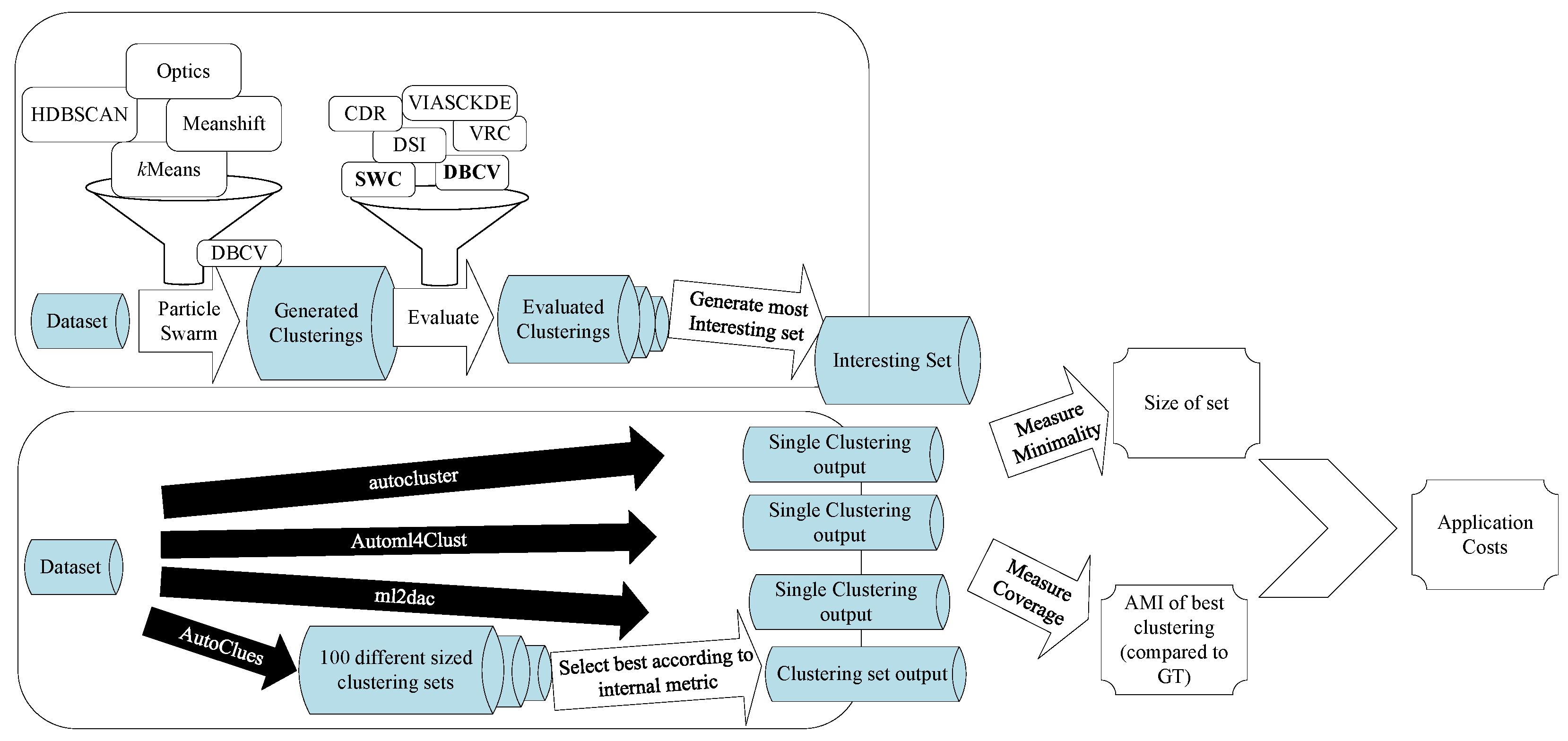
We will start this section by outlining the usual lifecycle of Automated Clustering before we describe the problems associated with this approach and by following up with the concrete problem definition. Whilst we know that there exist multiple areas of clustering with different goals like fuzzy [26] or hierarchical clustering [54], we will solely focus on the field of partitioning a dataset, meaning every single object will be assigned exactly one label assigning the object to exactly one cluster or identifying it as noise. This is not due to a limitation of our approach, but to keep the focus of this paper on our novel approach without the deviations of properties used in different situations. In fact, our methodology is agnostic to the actual used clustering algorithms, as long as a similarity between clusterings can be modelled and some quality metrics can compare them fairly. In this paper, we want to focus on the problem of AEC and specifically on the selection of an interesting set of clusters instead of describing a possible framework as a solution in detail. For this reason, we will consider some practical context-important parts like clustering generation, usage of different distance functions, and preprocessing steps, as black boxes for this paper, and we will provide an overview of the utilized algorithms together with the description of our experiments.

3.1. AutoML Lifecycle

The general goal of AutoML can be considered to be solving the Combined Algorithm Selection and Hyperparameter Optimization (CASH) [4] problem, i.e., finding both the perfect algorithm and hyperparameters for a user’s problem. This takes the cumbersome activity of fitting a good machine learning model from a data scientist to a computer and hence enables more inexperienced users to find good solutions.

Definition 1 

(CASH-Problem). Given a clustering $\mathrm{c}$, a Quality function on a solution $\mathrm{Q}\left(\mathrm{c}\right)$, an algorithm ${\mathrm{A}}^{\mathrm{i}}\in \mathcal{A}$, and ${\mathsf{\Lambda }}^{\mathrm{i}}$, the set of possible hyperparameters for ${\mathrm{A}}^{\mathrm{i}}$, the CASH-Problem can be formulated as follows:

$$A_{{\lambda }^{*}}^{*}=\underset{A^i\in \mathcal{A},\lambda \in {\mathsf{\Lambda }}^i}{argmax}Q\left(A_{\lambda }^i\left(D\right)\right)=\underset{c\in \mathbb{U}}{argmax}Q\left(c\right),$$

(2)

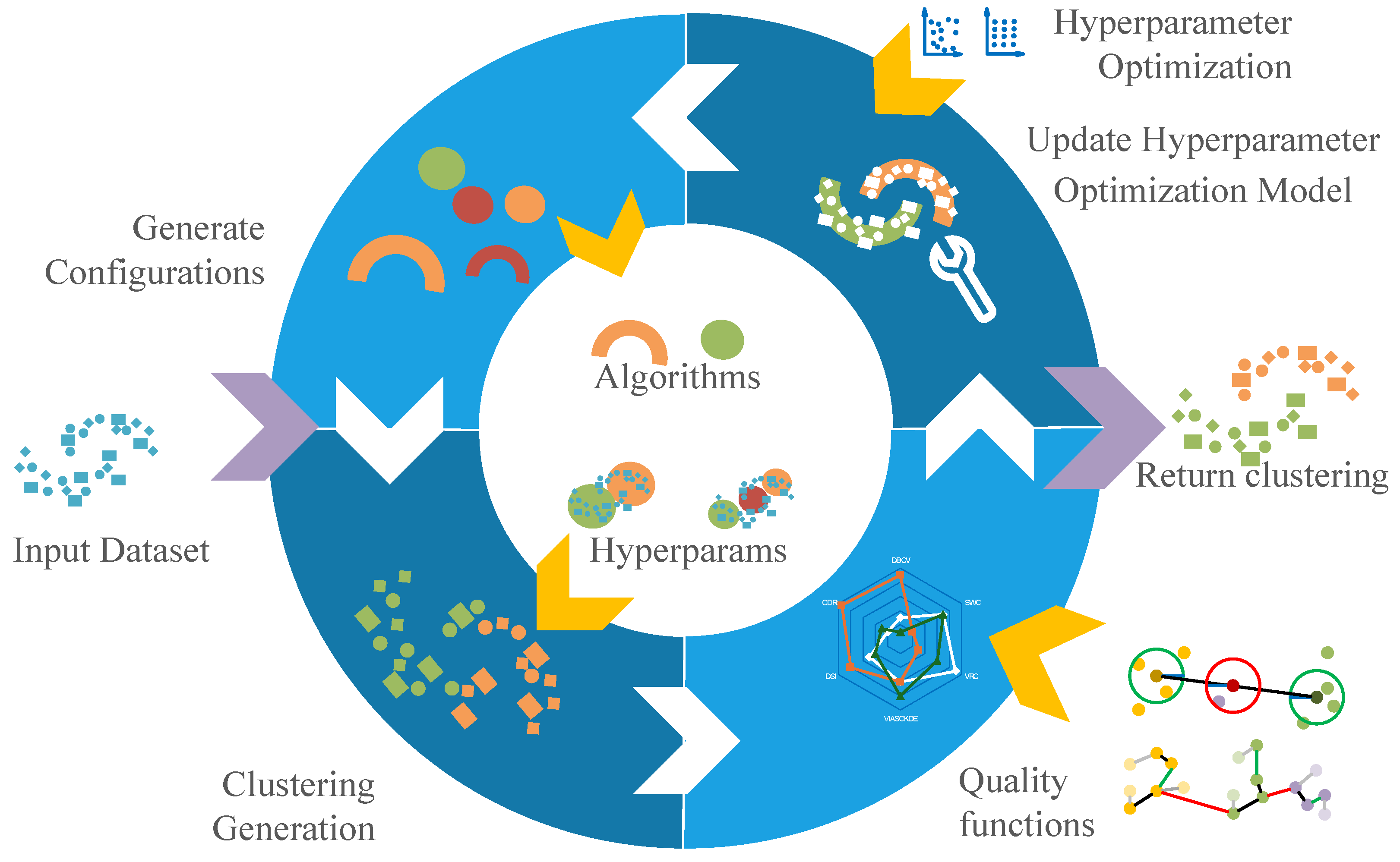
where ${\mathrm{A}}_{{\lambda }^{*}}^{*}$ is the optimal algorithm with the optimal parametrization ${\lambda }^{*}$, and $\mathbb{U}$ is the set of all investigated solutions.

In practice, many approaches try to solve this problem using an optimization cycle like the one illustrated in Figure 2. When using the framework, a user inputs a dataset and a time budget. The hyperparameter optimizer, Quality function, used algorithms, and their hyperparameter ranges are generally determined by the framework, although some frameworks also enable the user to make decisions on these. The optimizer will select promising combinations of algorithm and hyperparameters and use these to cluster the dataset. The goodness of these clusterings is measured by the Quality function. If the time budget is not exceeded, the optimizer will be updated based on the goodness of the previous clusterings. New algorithm and hyperparameter combinations are then chosen by the optimizer, where the values of the Quality function on the previous combinations are used to improve the quality. When no time is left, the best solution according to the Quality function is returned. In the current Automated Clustering literature, a solution is a single clustering of a dataset, whilst the Quality function is often either a single CVI [19,20], a consensus, or another combination of multiple CVIs [18].

Obviously, modern Automated Clustering approaches are more sophisticated and employ different techniques such as meta-learning or constraints given by the user, but for this paper, this abstraction will suffice to display our criticism on this model and to define the differences to our AEC problem. Clustering can be used for different tasks [15]. On the one hand, in sophisticated machine learning pipelines, clustering is often used as a preprocessing step and the quality (or usefulness) of a clustering can be evaluated by evaluating the effect of the clustering on the performance of the complete pipeline (if it can be measured). On the other hand, clustering is often used as an exploratory technique to find new insights in the structures of the data. Here, it is not possible to objectively evaluate the usefulness of a clustering, since the same insight might be very useful for one practitioner but trivial or even completely meaningless for another. 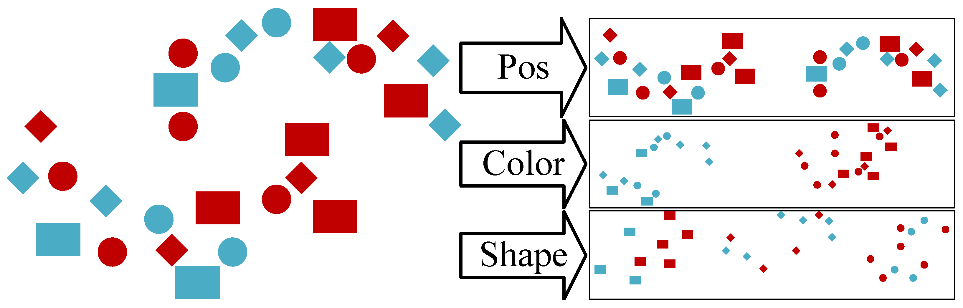Some consider that a “natural” clustering exists on any dataset [55]. However, this is, even if true, very dependent on the used distance and the notion of similarity, which are both non-trivial choices even for experienced data scientists. Consider for example the dataset in Figure 3, where every object has three properties as follows: position, shape, and colour. Without any further information, we can see three clear “natural” clusterings, where one is based on the position, one on the colour, and one on the shape. These clusterings all can be viewed as “correct”, but they are three completely different clusterings with not even the same number of clusters. One could even argue that all combinations of these clusters, resulting in 12 different clusters, would be the “natural” clustering. Without any specification by the data scientist, it cannot be known which of these clusterings is the most interesting for them.

Following this, we conclude that an Automated Clustering for exploratory data analysis has to provide a set of clusterings rather than a single clustering.

3.2. Theoretical Definition

The goal of AEC should be, to generate a set of multiple unique clusterings, each of which has the potential to be useful. However, on the other hand, this set should be as small as possible, since every cluster has to be investigated by a domain expert. As opposed to classical Automated Clustering, we will not search for a single clustering but a set of clusterings as the result of an AEC search. To find the “best” set of clusterings, we will define an interestingness measure, which needs to be optimized. This interestingness could also be used as a Quality function in our abstract AutoML lifecycle. However, in the scope of this paper, we generate the clusterings in a traditional Automated Clustering fashion (optimizing a single CVI) and select the resulting sets based on all clusterings generated during the training phase. For this reason, the methods in this paper might also be thematically close to the field of diversification (see, e.g., [50]). However, as our focus lies on the problem of finding a good interestingness to directly optimize the clustering sets, future research should divert from the field focused on a posteriori analysis. In contrast to our previous conference paper [25], we streamlined the necessary functions and omit the previously used usefulness function. While this leads to many definitions being different, it does not change any significant content.

The following notation is summarized in

Table 1. Used notations.

Notation	Definition
$\mathbb{U}$	Set of all clusterings
$c\in \mathbb{U}$	Clustering
$\mathcal{P}\left(\mathbb{U}\right)$	Power set of $\mathbb{U}$
$C\subseteq \mathbb{U},C\in \mathcal{P}\left(\mathbb{U}\right)$	Set of clusterings
$Q\left(c\right):\mathbb{U}\to {\mathbb{R}}^k,k\in \mathbb{N}$	Quality function
$I\left(C\right):\mathcal{P}\left(\mathbb{U}\right)\to \mathbb{R}$	Interestingness function
$S\left(C\right):C\to \mathcal{P}\left(C\right)$	Skyline function
$r\left(v\right):{\mathbb{R}}^k\to \mathbb{R},k\in \mathbb{N}$	Reduction function
$sim(c,o):\mathbb{U}\times \mathbb{U}\to \mathbb{R}$	Similarity function

for a quicker overview. We will denote $\mathbb{U}$ as the set of all (investigated) clusterings and $c\in \mathbb{U}$ as a single clustering. The power set of all clusterings will be denoted as $\mathcal{P}\left(\mathbb{U}\right)$ and a set of all investigated clusterings as $C\in \mathcal{P}\left(\mathbb{U}\right)$.

Definition 2 

(Quality Function). The Quality function is defined as the vector of evaluation results of a single clustering:

$$Q\left(c\right):\mathbb{U}\to {\mathbb{R}}^k,k\in \mathbb{N}.$$

(3)

The Quality function outputs a vector of scalars, and in our example, this will be a number of different CVI evaluations for the clustering. The Quality function can be arbitrarily complex, so a measure combining multiple CVI can also be a single component of the quality vector.

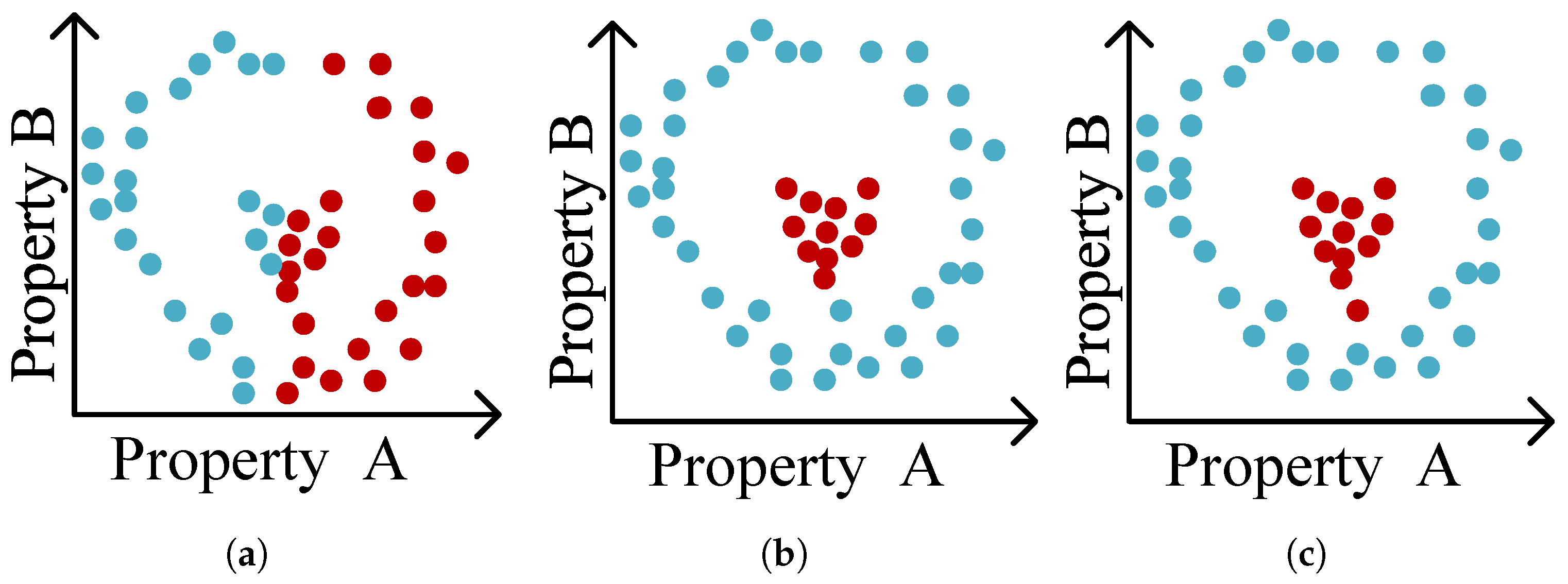
To be interesting in a set of clusters, a cluster must not only be “good” to some extent (most likely measured by a Quality function) but also unique in some kind of way. If we consider the three clusterings in Figure 4, we can see that two of these three (Figure 4b,c) clusterings have a very strong similarity and only differ in the labelling of one object, whilst the other clustering (Figure 4a) is vastly different. If we need to select two clusters from this set, it would grant little to no extra value for a practitioner if these clusters are as shown in Figure 4b,c, since it is highly unlikely that the single changed object will lead to many new insights. The other clustering, however, even while intuitively “worse” than the other two, would grant more insight as an addition to the other clustering (furthermore, it might even be the better fitting clustering, if Property B turns out to be irrelevant.). For this reason, the Interestingness function will need to weight the novelty and the quality of a clustering.

Definition 3 

(Interestingness function). The Interestingness function defines the likely interestingness of a set of clusterings to a practitioner as follows:

$$I\left(C\right):\mathcal{P}\left(\mathbb{U}\right)\to \mathbb{R}$$

(4)

In the end, the Interestingness function defines which sets of clusterings will be selected. For this reason, finding a good Interestingness function, most likely employing Q, will be a main goal in the field of AEC. Before we propose and investigate different Interestingness functions, we will first provide a formal definition of the AEC problem.

Definition 4 

(AEC Problem). The Automated Exploratory Clustering problem is to find an Interestingness function $\mathrm{I}$ such that the set $\mathrm{t}$ of clusterings, which is defined as

$$t=\underset{C\in \mathcal{P}\left(\mathbb{U}\right)}{argmax}I\left(C\right),$$

(5)

satisfies minimality, i.e., $\left|\mathrm{t}\right|$ is minimal, and coverage, i.e., $\mathrm{t}$ contains all relevant clusterings.

As can be seen in the definition above, the problem of Automated Exploratory Clustering is to find an appropriate Interestingness function that minimizes the set of relevant clusterings. While this problem definition is not tied to any specific application domain, it can accommodate various notions of interestingness and thus it is generally difficult to identify suitable characteristics. The following Corollary summarizes the characteristics for a well-chosen Interestingness function.

Corollary 1. 

A well-chosen Interestingness function $\mathrm{I}$ epitomizes the following properties:

1. 

All clusterings in $\mathrm{t}$ are different.

2. 

The set $\mathrm{t}$ is much smaller than the set of all clusterings, i.e., $\mathrm{t}\ll \left|\mathbb{U}\right|$.

3. 

Any two clusterings in $\mathrm{t}$ exhibit a sufficient degree of dissimilarity.

4. 

The set $\mathrm{t}$ is the smallest set containing all relevant clusterings.

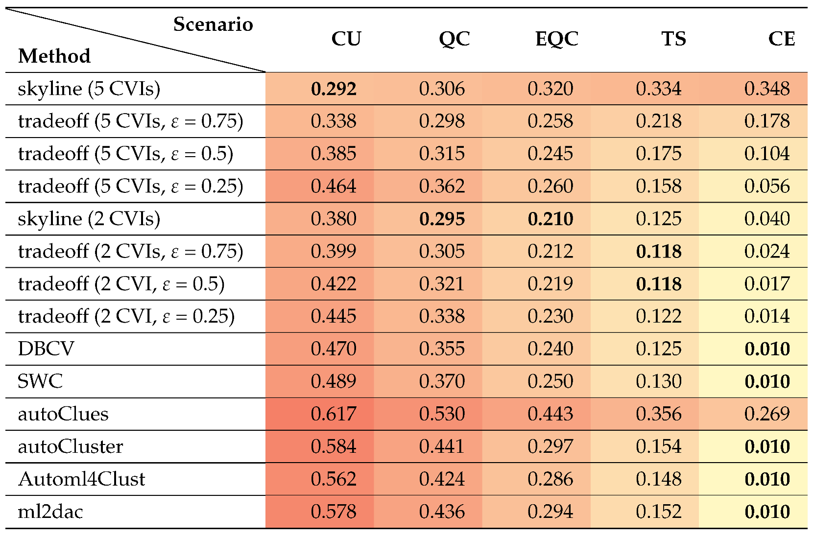
Based on the definition of the AEC problem, we propose three different Interestingness functions which aim for (i) minimality, (ii) coverage, and (iii) tradeoff between both. The first Interestingness function, introduced in Section 3.3, optimizes minimality by returning a single clustering like in traditional Automated Clustering approaches, while the second function, presented in Section 3.4, optimizes coverage by returning all clusterings regarded important by several CVIs, regardless of their similarity among each other. Finally, the Interestingness function proposed in Section 3.5 balances the tradeoff between minimality and coverage by taking a skyline and pruning similar clusterings.

Without loss of generality, we assume for all subsequent Interestingness functions that the Quality function $Q\left(c\right)$ of a single clustering $c\in \mathbb{U}$ is to be maximized in all components, and all resulting values are non-negative (as a minimized value can be multiplied by −1 in order to be maximized and normalization can ensure that all values are greater than 0 by an addition with a constant c).

3.3. Conventional Automated Clustering

Considering the minimality in Definition 4, the easiest way to optimize in this regard (apart from returning an empty set) is to always only return a single element. This is carried out by many conventional Automated Clustering methods like autoCluster [18], Automl4Clust [19], or ml2dac [20]. The idea of returning a single clustering is formally defined in terms of an Interestingness function as shown in the definition below. For this purpose, me make use of a reduction function R that reduces multiple CVIs into a scalar value.

Definition 5 

(Single-Return Interestingness). Let $\mathrm{R}\left(\mathrm{v}\right):{\mathbb{R}}^{\mathrm{k}}\to \mathbb{R}$ be any reduction function, the Single-Return Interestingness function is defined as follows:

$$I\left(C\right)=\left\{\begin{array}{cc}R\left(Q\right(c\left)\right),\hfill & \mathit{if} \left|C\right|=1 (\mathit{with} C=\{c\left\}\right)\hfill \\ -1,\hfill & otherwise\hfill \end{array}\right.$$

(6)

It can be seen that the function $I\left(C\right)$ is negative for all sets of clusterings with $\left|C\right|>1$ and only singleton sets consisting of one clustering have positive values of $Q\left(c\right)$, where $c\in C$ is the sole clustering in the set. With this interestingness, a single clustering, which is regarded “best” by means of the Quality function Q, will be returned. This scenario is just a reformulation of the conventional Automated Clustering case, where arbitrary complex (combinations of) CVIs are used to select a single best clustering. For example, $R\left(v\right)$ can just be a simple reduction like the average, maximum, or minimum of a number of CVIs. However, it can also be an arbitrary complex combination of those.

3.4. Skyline Operator

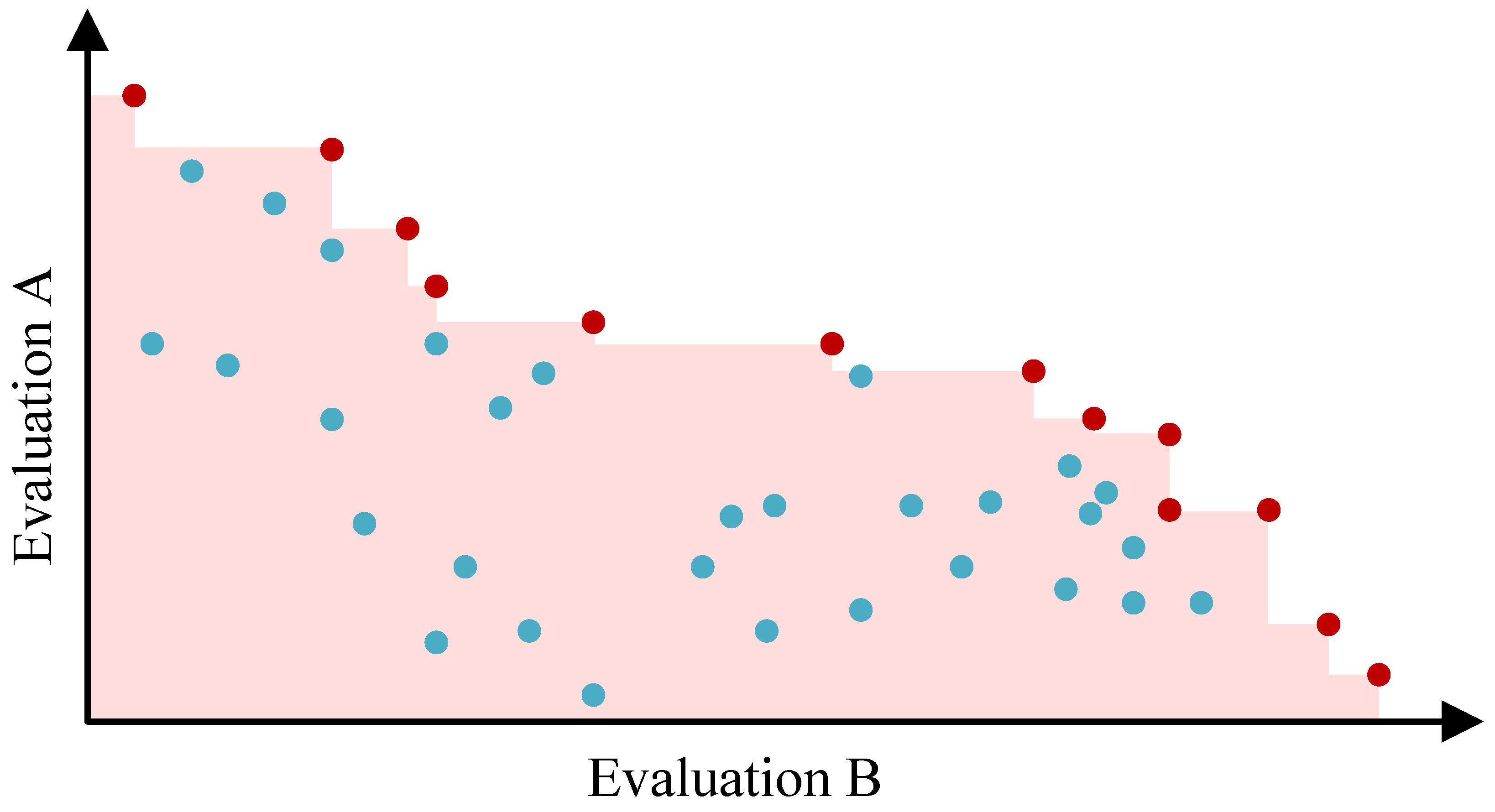
If we want to optimize the coverage, we need to include all clusterings that are somewhat interesting. A common approach for this is to determine the skyline or Pareto set of all clusterings, which comprises every clustering that is not dominated in every CVI by another clustering [56]. The resulting clusterings are considered to be interesting, as also visualized by means of an example of a skyline, indicated by red objects, in Figure 5. The underlying concept of domination is formalized in the following definition.

Definition 6 

(Domination). Let $\mathrm{c},\mathrm{d}\in \mathbb{U}$ be two clusterings. The clustering $\mathrm{c}$ dominates $\mathrm{d}$ according to a Quality function $\mathrm{Q}$, if it is worse in no single dimension and superior in at least one as follows [57]:

$$c{\succ }_{Q}d\iff \forall i:Q{\left(c\right)}_i\ge Q{\left(d\right)}_i\wedge \exists j:Q{\left(c\right)}_j>Q{\left(d\right)}_j$$

(7)

Based on the definition of domination among clusterings, we can now define a skyline or Pareto-optimal subset as follows:

Definition 7 

(Skyline). Let $\mathrm{C}$ be a set of objects and $\mathrm{Q}$ a Quality function. The Skyline $\mathrm{S}\left(\mathrm{C}\right)\in \mathcal{P}\left(\mathrm{C}\right)$ is defined as follows:

$$S\left(C\right)=\{c\in C| \nexists d\ne c,d\in C:d{\succ }_{Q}c\}$$

(8)

It is evident that the size of the skyline is only limited by the size of the input dataset and can be independent of the number of CVIs. However, every clustering which seems to be the “best” according to one component of the Quality function Q or a combination of components will be part of the skyline. It is easy to construct an Interestingness function that will directly lead to the skyline set being returned.

Definition 8 

(Skyline interestingness). Using the skyline defined in Definition 7, we define the skyline Interestingness function as follows:

$$I\left(C\right)=\left\{\begin{array}{cc}\left|C\right|\hfill & ,C=S\left(C\right)\hfill \\ -1\hfill & ,else\hfill \end{array}\right.$$

(9)

While this method gives a maximal coverage (according to the Quality function inherently utilized in the skyline $S\left(C\right)$), the resulting skylines can be extensive and exhibit significant redundancy wrt. to similarity of the contained clusterings. This issue is addressed via the subsequent Interestingness function.

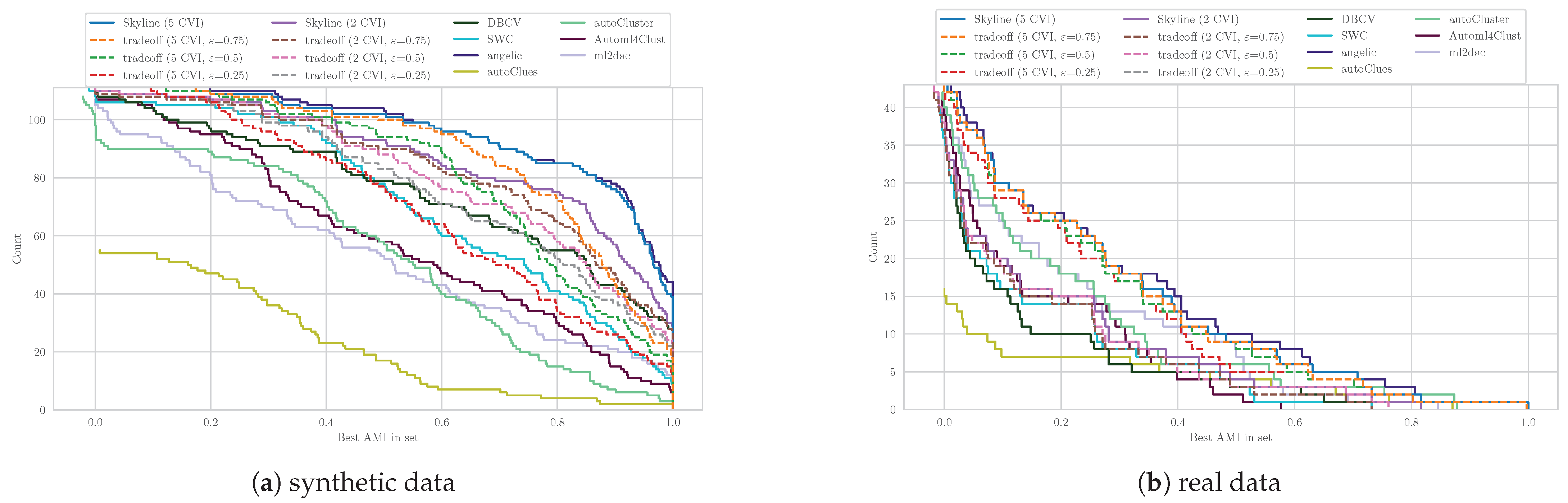
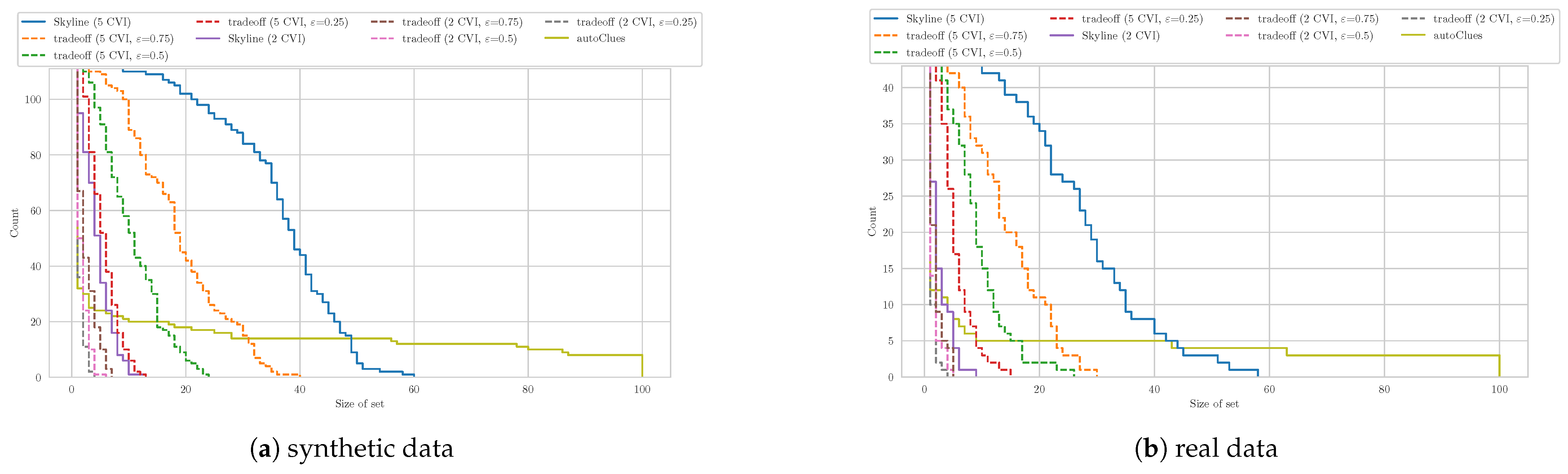
3.5. Similarity-Based Tradeoff

As we have now seen two variants, which optimize the two different goals of Definition 4, we will now propose a third Interestingness function that exactly balances the aforementioned tradeoff. While it will still use the skyline to get a high coverage, we will prune similar clusterings to ensure a much smaller resulting set.

Definition 9 

(Similarity-pruned interestingness). Using the skyline defined in Definition 7 and a similarity function $\mathrm{sim}:\mathrm{C}\mapsto [0,1]$, we can define the following:

$$I(C,\epsilon )=\left\{\begin{array}{cc}\left|C\right|\hfill & ,C=S\left(C\right)\wedge \forall o\ne c\in C:sim(c,o)<\epsilon \hfill \\ -1\hfill & ,else\hfill \end{array}\right.$$

(10)

We will get the biggest possible subset of the skyline, in case there are no two elements which have a higher similarity value than $\epsilon$. Using this, we can control the tradeoff between minimality and coverage by adapting $\epsilon$, as a value close to zero will eliminate most clusterings and only leave a small subset, while a high value of $\epsilon$ will retain the complete skyline.

It can be seen that both methods mentioned earlier are in fact only special parametrisations of this approach. Setting the $\epsilon =1$ will lead to all clusterings in the skyline being selected, while setting $\epsilon =0$ will grant only one clustering (provided an apt method to handle ties is added).

The choice of the similarity function of two clusterings will have a significant impact on this result. Possible choices include the ARI [58] or the AMI [51]. However, any external CVI can be used. The creation of this set is similar to the motley algorithm used in the field of diversification [50,59]. However, in that field, the size of the resulting set is fixed instead of the threshold parameter.

This set can be approximated more efficiently by a greedy algorithm shown in Algorithm 1. We start to build the set with the skyline element with the minimal highest similarity to any other clustering in the skyline. Following this, we expand the resulting set with the clustering, which has the minimal highest similarity to any selected clustering. We stop this once no clustering is left. In l. 1–3, the skyline set S is built, and for every clustering, the highest similarity to any other clustering is stored. In l.4–7, the starting element is selected and stored in the target set t, while the remaining set $rest$ is initialized and the current minimal maximal similarity $sim$ to any object in the rest set is initialized to 0. While this similarity is smaller than $\epsilon$ (hence there still are clusterings in $rest$ with a similarity less than $\epsilon$ to all clusterings to t), an addition of new clusterings to the target set is evaluated (l. 8–16). The array $ma{x}_{s}ims$ is updated to reflect the maximal similarity to any object in the t set for every object in $rest$, and the clustering with the minimal maximum similarity is selected for as the next new element $new\_index$ (l. 9–10). If the similarity of this object to any object in t is smaller than $\epsilon$, the element is added to set t (l. 11–15); otherwise, the resulting set is returned (l. 17).

The time complexity lies in $\mathcal{O}(n^3+n^2·\mathcal{O}\left(s\right))$. The first part (l.1–7) has a complexity of $\mathcal{O}(n^2·\mathcal{O}\left(s\right))$, as every similarity between two clusterings must be computed. The following while loop (l. 8–16) can happen up to n times, as all clusterings can be less similar than the threshold. The time complexity of assigning each element in the remaining set the maximum similarity of a set in the target set (l. 9) is in $\mathcal{O}\left(n^2\right)$. For this reason, the complexity of the for loop is in $\mathcal{O}\left(n^3\right).$ The main space requirement for this algorithm are the pairwise similarities. For this reason, the space complexity is in $\mathcal{O}\left(n^2\right)$.

Algorithm 1 An algorithm to greedy approximate the tradeoff set

Input: Clusterings $\mathbb{U}$, Interestingness Function S, threshold $\epsilon$, Clustering similarity function s Output: most interesting set t   1: $n\leftarrow \left|\mathbb{U}\right|$   2: $S\leftarrow S\left(\mathbb{U}\right)$                      ▹ S according to Q   3: $\forall i\in \mathbb{U}:max\_sim{s}_i\leftarrow {max}_{x\ne i\in \mathbb{U}}\left(s(i,x)\right)$   4: $start\_index\leftarrow {argmin}_{i\in \mathbb{U}}(max\_sim{s}_i)$   5: $sim\leftarrow 0$   6: $t\leftarrow \left\{\mathbb{U}\right[start\_index\left]\right\}$   7: $rest\leftarrow \mathbb{U}\setminus \left\{t\right\}$   8: while  $sim\le \epsilon$  do   9:       $\forall i\in rest:max\_sim{s}_i\leftarrow {max}_{x\in t}\left(s(i,x)\right)$ 10:       $next\_index\leftarrow {argmin}_{i\in rest}(max\_sim{s}_i)$ 11:       $sim\leftarrow max\_sim{s}_{next\_index}$ 12:       if $sim\le \epsilon$ then 13:         $t\leftarrow t\cup \{next\_index\}$ 14:         $rest\leftarrow \mathbb{U}\setminus \left\{t\right\}$ 15:       end if 16: end while 17: return  t

4. Experimental Works

In our experiments, we simulated a simple AutoML pipeline. In the first step, multiple algorithms (Section 4.2) are used to generate a multitude of clusterings on different real and synthetic datasets (Section 4.1). The parameters are optimized using hyperparameter tuning based on a single CVI. Multiple CVI are used to evaluate every resulting clustering, cf. Section 4.3. The concrete way of how these CVIs are used to evaluate the interestingness of the clusterings according are shown in Section 4.4. In order to showcase the methods in different scenarios, we propose a measure for the application cost (Section 4.5). We also evaluated and compared different state-of-the-art methods (Section 4.6). A short overview over both our pipeline and the used reference methods is depicted in Figure 6.

4.1. Datasets

We used different real and synthetic datasets for our experiments. For the real datasets, we used the six datasets mentioned in [60] as well as forty datasets from the UCI-Repository [61], which were selected by [62]. We also used [62] for the 136 synthetic datasets. Of these synthetic datasets, 53 have arbitrary, non-convex shapes; 43 have overlapping clusters; and 10 contain outliers. An extensive table of the datasets used can be found in the Appendix A in

Table A1. Used datasets for the evaluation in this paper. Group denotes the source of the dataset, arb indicates if the dataset has an arbitrary shape, out if it contains outliers, and ovl if the clusters have overlaps.

Name	Group	n	$\mathit{\delta }$	$\left|\mathit{P}\right|$	$\left|\mathit{O}\right|/\mathit{n}$	arb	out	ovl
iris	dbcv	150	4	3	0.00	×	×	×
wine	dbcv	178	12	3	0.00	×	×	×
glass	dbcv	214	7	6	0.00	×	×	×
kdd	dbcv	600	60	6	0.00	×	×	×
cell237	dbcv	237	16	4	0.00	×	×	×
cell384	dbcv	384	16	5	0.00	×	×	×
zoo	uci	101	16	7	0.00	×	×	×
led	uci	500	7	10	0.00	×	×	×
arrhythmia	uci	452	262	13	0.00	×	×	×
banknote	uci	1372	4	2	0.00	×	×	×
german	uci	1000	24	2	0.00	×	×	×
balance-scale	uci	625	4	3	0.00	×	×	×
spambase	uci	4601	57	2	0.00	×	×	×
seeds	uci	210	7	3	0.00	×	×	×
waveform3	uci	5000	21	3	0.00	×	×	×
wdbc	uci	569	31	2	0.00	×	×	×
tae	uci	151	5	3	0.00	×	×	×
iris	uci	150	4	3	0.00	×	×	×
wine	uci	178	13	3	0.00	×	×	×
musk	uci	6598	166	2	0.00	×	×	×
pima	uci	768	8	2	0.00	×	×	×
sonar	uci	208	60	2	0.00	×	×	×
balance	uci	625	4	3	0.00	×	×	×
ecoli	uci	336	7	8	0.00	×	×	×
heart	uci	303	13	2	0.00	×	×	×
ionosphere	uci	351	30	2	0.00	×	×	×
liver	uci	345	6	2	0.00	×	×	×
unbalance	uci	6500	2	8	0.00	×	×	×
letter	uci	5000	16	26	0.00	×	×	×
cpu	uci	209	6	116	0.00	×	×	×
msplice	uci	3175	240	3	0.00	×	×	×
wineqr	uci	1599	11	6	0.00	×	×	×
dermatology	uci	358	34	4	0.00	×	×	×
vehicle	uci	846	18	4	0.00	×	×	×
vote	uci	435	16	2	0.00	×	×	×
landsat	uci	2000	36	6	0.00	×	×	×
thyroid	uci	215	5	3	0.00	×	×	×
haberman	uci	306	3	2	0.00	×	×	×
biodeg	uci	1055	41	2	0.00	×	×	×
wpbc	uci	198	33	2	0.00	×	×	×
dna	uci	2000	180	3	0.00	×	×	×
glass	uci	214	9	6	0.00	×	×	×
breast	uci	277	9	2	0.00	×	×	×
segment	uci	2310	18	7	0.00	×	×	×
eeg	uci	14,980	14	2	0.00	×	×	×
D31	syn	3100	2	31	0.00	×	×	✓
twomoon	syn	180	3	2	0.00	×	×	×
target	syn	770	2	6	0.00	✓	×	×
banana-Ori	syn	4811	2	2	0.00	✓	×	×
st900	syn	900	2	9	0.00	×	×	✓
disk-4600n	syn	4600	2	2	0.00	✓	×	×
disk-6000n	syn	6000	2	2	0.00	✓	×	×
ds3c3sc6	syn	905	2	6	0.00	✓	×	✓
spherical_5_2	syn	250	2	5	0.00	×	×	✓
threenorm	syn	1000	2	2	0.00	×	×	✓
ds4c2sc8	syn	485	2	8	0.00	×	×	✓
S2	syn	5000	2	15	0.00	×	×	✓
DS-850	syn	850	2	5	0.00	×	×	×
3MC	syn	400	2	3	0.00	×	×	×
2d-4c-no9	syn	876	2	4	0.00	×	×	✓
D1	syn	87	2	3	0.00	×	×	×
longsquare	syn	900	2	6	0.00	×	×	×
pearl	syn	1000	2	2	0.00	✓	×	×
xclara	syn	3000	2	3	0.00	×	×	×
chainlink	syn	1000	3	2	0.00	×	×	×
long1	syn	1000	2	2	0.00	×	×	×
fourty	syn	1000	2	40	0.00	×	×	×
2spiral	syn	1000	2	2	0.00	✓	×	×
aggregation	syn	788	2	7	0.00	×	×	✓
cassini	syn	1000	2	3	0.00	×	×	×
ds2c2sc13	syn	588	2	13	0.00	×	×	×
dartboard1	syn	1000	2	4	0.00	✓	×	×
square2	syn	1000	2	4	0.00	×	×	✓
jain	syn	373	2	2	0.00	✓	×	×
spiralsquare	syn	1500	2	6	0.00	✓	×	×
flame	syn	240	2	2	0.00	✓	×	×
elliptical_10_2	syn	500	2	10	0.00	×	×	✓
2dnormals	syn	1000	2	2	0.00	×	×	✓
disk-1000n	syn	1000	2	2	0.00	✓	×	✓
donutcurves	syn	1000	2	4	0.00	✓	×	×
cluto-t7-10k	syn	10,000	2	10	0.08	✓	✓	×
dpb	syn	4000	2	6	0.16	✓	✓	✓
cure-t2-4k	syn	4200	2	7	0.05	✓	✓	✓
square3	syn	1000	2	4	0.00	×	×	✓
spiral	syn	312	2	3	0.00	✓	×	×
square4	syn	1000	2	4	0.00	×	×	✓
square1	syn	1000	2	4	0.00	×	×	✓
diamond9	syn	3000	2	9	0.00	×	×	✓
zelnik6	syn	238	2	3	0.00	✓	×	×
DS5	syn	500	2	5	0.00	×	×	×
wingnut	syn	1016	2	2	0.00	×	×	×
twodiamonds	syn	800	2	2	0.00	×	×	×
spherical_4_3	syn	400	3	4	0.00	×	×	×
sizes2	syn	1000	2	4	0.00	×	×	✓
DS6	syn	800	2	4	0.00	×	×	✓
banana	syn	4811	2	2	0.00	✓	×	×
tetra	syn	400	3	4	0.00	×	×	×
complex8	syn	2551	2	8	0.00	✓	×	×
triangle2	syn	1000	2	4	0.00	×	×	×
zelnik3	syn	266	2	3	0.00	✓	×	×
sizes5	syn	1000	2	4	0.00	×	×	✓
disk-4000n	syn	4000	2	2	0.00	✓	×	×
donut1	syn	1000	2	2	0.00	×	×	×
cure-t1-2000n-2D	syn	2000	2	6	0.00	×	×	×
2d-3c-no123	syn	715	2	3	0.00	×	×	✓
cuboids	syn	1002	3	4	0.00	×	×	×
cluto-t5-8k	syn	8000	2	7	0.14	✓	✓	×
zelnik5	syn	512	2	4	0.00	×	×	×
R15	syn	600	2	15	0.00	×	×	×
cure-t0-2000n-2D	syn	2000	2	3	0.00	×	×	×
disk-3000n	syn	3000	2	2	0.00	✓	×	×
spherical_6_2	syn	300	2	6	0.00	×	×	×
dpc	syn	1000	2	6	0.15	✓	✓	×
zelnik1	syn	299	2	3	0.00	✓	×	×
2d-10c	syn	2990	2	9	0.00	×	×	✓
3-spiral	syn	312	2	3	0.00	✓	×	×
disk-4500n	syn	4500	2	2	0.00	✓	×	×
D13	syn	588	2	13	0.00	×	×	×
s-set1	syn	5000	2	15	0.00	×	×	✓
square5	syn	1000	2	4	0.00	×	×	✓
cluto-t4-8k	syn	8000	2	7	0.10	✓	✓	×
compound2	syn	399	2	6	0.00	✓	×	×
pmf	syn	649	3	5	0.00	×	×	×
blobs	syn	300	2	3	0.00	×	×	✓
cluto-t8-8k	syn	8000	2	9	0.04	✓	✓	×
donut3	syn	999	2	3	0.00	✓	×	×
S4	syn	5000	2	15	0.00	×	×	✓
long2	syn	1000	2	2	0.00	×	×	×
DS-577	syn	577	2	3	0.00	×	×	✓
dense-disk-5000	syn	5000	2	2	0.00	✓	×	×
D2	syn	85	2	4	0.00	×	×	×
sizes4	syn	1000	2	4	0.00	×	×	✓
disk-5000n	syn	5000	2	2	0.00	✓	×	×
gaussians1	syn	100	2	2	0.00	×	×	×
elly-2d10c13s	syn	2796	2	10	0.00	×	×	✓
sizes3	syn	1000	2	4	0.00	×	×	✓
2d-4c-no4	syn	863	2	4	0.00	×	×	×
cure-t2-4k1	syn	4000	2	6	0.00	×	×	✓
zelnik4	syn	622	2	5	0.22	✓	✓	×
curves1	syn	1000	2	2	0.00	×	×	×
zelink6	syn	238	2	3	0.00	×	×	×
zelink1	syn	299	2	3	0.00	✓	×	×
lsun	syn	400	2	3	0.00	×	×	×
S3	syn	5000	2	15	0.00	×	×	✓
sizes1	syn	1000	2	4	0.00	×	×	✓

. Here, we only give a brief overview in (

Table 2. Dataset overview.

Group	min n	max n	min d	max d	min $\left|\mathit{P}\right|$	max $\left|\mathit{P}\right|$
Real	101	14,980	2	262	2	116
Synthetic	30	10,000	2	3	1	40

), where n is the number of objects, d is the number of dimensions, and $\left|P\right|$ is the number of clusters in the dataset.

4.2. Clustering Algorithms

To generate different clusterings with different characteristics, we used four clustering algorithms. These algorithms all have particular intrinsic notions of a clustering. We selected these algorithms to represent different notions of clusterings. An overview of these algorithms is given in

Table 3. Used clustering algorithms.

Name	Used Parameters	Found Shapes
kMeans	$\mathtt{k}\in [2,30]$	globular clusters around a centroid
HDBSCAN	$\mathtt{min}\_\mathtt{cluster}\_\mathtt{size}\in [2,30]$	arbitrary shapes of similar density
Meanshift	$\mathtt{bandwidth}\in [0.1,50]$	fields of smooth density
OPTICS	$\mathtt{xi}\in [0.025,0.5],\mathtt{min}\_\mathtt{samples}\in [3,20]$	arbitrary shapes of similar density

. All algorithms have parameters, which we fine-tuned using the Particle Swarm [63] method to optimize the DBCV value. We used the implementation of [64] for the hyperparameter optimization. We used a swarm size of 10 and a generation number of 3, leading to 30 different clusterings per dataset and algorithm, out of which we pruned double clusterings.

The classical kMeans [11] algorithm produces clusterings consisting of spherical, convex clusters without noise. k centroids are determined, and every object is assigned to the closest centroid, resulting in k clusters. The centroids and assignments are updated iteratively until convergence. We used the implementation in [65] and set the bounds for k to the interval $[2,30]$.

HDBSCAN [13] assigns clusters to objects based on the distance to other objects. The approach is linkage-based and finds clusterings of aribtrary shapes. In this paper, we used the implementation of [66], where we tuned the parameter min_cluster_size in the interval $[1,30]$.

The Meanshift [14] algorithms sets centroids in the mean of a region of points. We used the implementation of [65], where we set the bounds for bandwidth to the interval $[0.1,50]$.

The OPTICS [30] algorithm is a density-based approach similar to HDBSCAN. When all reachabilities are computed, a cut on these is made to generate the clusters. We used the implementation in [65] and set the bounds for xi to $[0.025,0.5]$ and for min_samples to $[3,20]$.

4.3. Quality Functions

In order to evaluate the clusterings, we chose six different CVIs according to the results in [67] as a Quality function. Like our chosen clustering algorithms, these CVIs encourage different notions of clusterings in their evaluations. The utilized Quality functions are described below in

Table 4. Used CVIs.

Name	Found Shapes	Optimization
SWC	Globular clusters	↑
DBCV	Arbitrary shapes with no overlap	↑
DSI	Distinct difference of distances	↑
CDR	Arbitrary-shaped	↓
VIASCKDE	Arbitrary shapes	↑
VRC	Globular clusters	↑

.

The Silhouette Width Criterion (SWC) [52]—also known as Silhouette Coefficient—computes a silhouette for each object based on the average distance to objects in its own cluster and the average distance to objects in the second closest cluster. Non-convex clusters are valued highly using this method. We used the implementation in [65].

Density-Based Clustering Validation (DBCV) [60] is an MST-based measure using the density of an object in its cluster. We use our own implementation (available at https://github.com/g-schlake/ASCVI accessed at 19 May 2025), which matches the results of the original authors’ implementation on the given test datasets.

The Density Separability Index (DSI) [68] compares the histograms of distances between a cluster and objects of all other clusters. We use the original authors’ implementation (available at https://github.com/ShuyueG/CVI_using_DSI accessed at 19 May 2025).

For the Contiguous Density Region (CDR) [69], the density of objects measured by the distance to its nearest neighbour is measured. Clusters should be regions where this density is constant. We used our own implementation (available at https://github.com/g-schlake/ASCVI accessed at 19 May 2025), which matches the implementation of the original authors.

Validity Index for Arbitrary-Shaped Clusters Based on the Kernel Density Estimation (VIASCKDE) [70] is an index similar to the SWC, but in this approach, objects are also weighted by the density assigned by a Kernel Density Estimation (KDE) on the dataset to value objects in dense areas higher. We used the original authors’ implementation (available at https://github.com/senolali/VIASCKDE accessed at 19 May 2025). To fit the KDE, we use a Gaussian Kernel and fit the bandwidth in a random search in the space in $[0.1,100]$.

The Variance Ratio Criterion (VRC) [71]—also known as Calinski–Harabasz criterion—is a classical metric using the trace of the dispersion matrices within each cluster and between clusters. We used the implementation in [65].

As not all CVIs can directly deal with objects assigned as outliers, we adopt the scores with a multiplication by ${\displaystyle \frac{n-\left|O\right|}{n}}$ for maximized and by ${\displaystyle \frac{n}{n-\left|O\right|}}$ for minimized CVIs, where $\left|O\right|$ is the number of outliers. We did this according to [67].

4.4. Interestingnesses’ Functions

We have defined multiple implementations (based on different Quality functions) for each method mentioned in Section 3. For the Single-Return Interestingness (Section 3.3), we used two different CVIs, the DBCV and the SWC, as these seem to deliver the best results and offer different notions of a good clustering. For the Skyline Interestingness function (Section 3.4), we used two combinations of CVIs. The first method used both aforementioned measures (DBCV and SWC) to build a skyline, while the second method used all six CVIs described in Section 4.3. For the Similarity-Pruned Interestingness function (Section 3.5), we use both aforementioned skylines as a base and values of $0.25,0.5$ and $0.75$ for the parameter $\epsilon$. As a similarity metric, we used the Adjusted Rand Index (ARI) [58] between two clusters, where we assigned every noise object to a singleton cluster to avoid noise being mistaken for a valid cluster.

4.5. Usage Scenarios

In order to gain insights on the effects of different strategies for different users, we create an application cost $ac$ for every clustering set. This application cost is dependent on $\left|C\right|$, the number of clusterings in the set; $ec$, an exploratory cost to model the effort to manually evaluate the clusterings for the practitioner; v, the value of the clustering, measured as the minimal distance of a clustering in the set to the optimal clustering (measured by the ground truth); and $uc$, a usability cost modelling the negative impact of a suboptimal clustering.

Definition 10 

(Application Cost). Let $\mathrm{C}$ be a set of clusterings on a dataset, $\mathbb{U}$ the set of all clusterings on the dataset, $\mathrm{gt}$ be the known best clustering for this dataset, and $\mathrm{sim}$ a similarity measure. We can define the application cost $\mathrm{ac}$ dependent on the exploratory cost $\mathrm{ec}$ and the usability cost $\mathrm{uc}$ as follows:

$$ac(C,gt,ec,uc)={\displaystyle \frac{\left|C\right|}{\left|U\right|}}·ec+\left(1-\underset{c\in C}{max}sim(c,gt)\right)·uc$$

(11)

Using this cost function, we can define different user scenarios, where the costs are distributed differently. This should make it possible to compare the methods under a variety of settings. Our parametrisations are shown in

Table 5. Different parameterisations for the Application Cost function.

Name	Abbr.	$\mathit{ec}$	$\mathit{uc}$
Costly Usability	CU	0	1
Thorough Search	TS	0.25	0.75
Equal costs	EQC	0.5	0.5
Quick Search	QS	0.75	0.25
Costly Evaluation	CE	1	0

.

In our scenario, we set $ec+uc=1$ to ensure $ac\in [0,1]$. However, this is not a fixed property of the application cost. We can see that our method CU only evaluates the quality of the best clustering, disregarding the size of the clustering set. On the other hand, CE only evaluates the size of the clustering set, without any regard to the quality reached by the set.

4.6. Compared Methods

While there does not (to our knowledge) exist another method directly comparable to our approach, we do benchmark three AutoML methods for clustering using the standard parameters and the implementation (available at https://github.com/biagiolicari/Benchmark_result_AutoML/tree/main accessed at 19 May 2025) of [2] on our datasets. We opted for the standard parameters, as we wanted to simulate a practitioner without knowledge in clustering, unable to select apt parameters. We used autoCluster [18], Automl4Clust [19], and ml2dac [20] (with all available meta-features), which, however, only output a single “best” clustering. In order to enable a fair comparison, we set the number of evaluations to 100, the same number used in our experiments. For this reason, every comparison has this big caveat, as a single shot must not always find all relevant clusterings. However, as only a single clustering is returned, the choice for the user is much easier. We omitted cSmartMl [44], as the implementation did not work in a wide variety of our results and suffered from a slow execution time.

We also include autoClues [21], adapting their public implementation (available at https://github.com/big-unibo/autoclues/ accessed at 19 May 2025), which first computes a number of clusterings and then selects the most promising and diverse set of k clusterings for a given k. We used the Adjusted Mutual Information as a target function according to the experiments conducted by the original authors. We computed the internal score for every $k\in [1,100]$ and selected the clustering set with the highest score. Again, this comparison has to be taken with a grain of salt, as this method was developed to be used with a fixed k. We could not set the number of executions for this method, so it has computed more than 100 clusterings for a number of datasets. On some other datasets, however, the method did not produce a single clustering as all clusterings have been pruned internally.

An overview of all (including our) methods and their used clustering algorithms and CVIs can be seen in

Table 6. Clustering algorithms and CVIs used in our pipeline and the compared methods (✓), implemented in the framework but not used in the default configuration and our experiments (✗). Our approach uses less methods than the competitors to avoid too similar clusterings.

	Method	Our Pipeline	autoClues	autoCluster	Automl4Clust	ml2dac
Algorithm/CVI
Clustering algorithms
kMeans		✓	✓ 1	✓ 1	✓ 1	✓ 1
kMedoids					✓
GMM			✓	✓	✓	✓
Meanshift		✓	✓	✗		✓
Affinity Propagation			✓	✗		✓
Agg. Clustering			✓	✓	✓	✓
Birch			✓	✓		✓
Spectral Clustering			✓	✓		✓
DBSCAN				✗		✓
OPTICS		✓	✓	✗		✓
HDBSCAN		✓
CVIs
DBI [72]			✗ 2	✓	✗	✓
VRC (CHI)		✓		✓	✗	✓
DI [73]						✓
SWC		✓	✓ 1	✓	✓	✓
DBCV		✓				✓
DSI		✓
CDR		✓
VIASCKDE		✓
CJI [74]						✓
COP [75]						✓

¹ including minibatch kMeans. ² autoClues also uses these CVI with a dimensionality reduction using t-SNE as preprocessing. In the experiments, SWC with t-SNE preprocessing is used.

.

5. Results

To evaluate the results of our experiments, we will evaluate, how well the two properties in Definition 4 (minimality and coverage) are met. For minimality, it is trivial to measure this based on the size of each retrieved clustering set. For coverage, we will treat the original labelling of the datasets as a kind of ground truth. We can safely assume, that a dataset interesting for a practitioner behaves similar to the assigned ground truth (note that this obviously does not mean that this ground truth is the only correct labelling for the dataset), so we can measure whether the most similar clustering to the ground truth is extracted. As we do not measure the quality of the clusterings generated, we will need to take the rank of the best clustering into consideration. In the third subsection, we evaluate our different application costs defined in Section 4.5 to see the performance of different methods in various scenarios.

5.1. Coverage

To evaluate whether good clusterings were selected, we look at the AMI [51] in comparison to the ground truth as proxy for the clustering desired by a user. In Figure 7, we show how many clusterings have a higher highest AMI than the x-axis refers to. In addition to the 10 approaches described earlier, we also plotted an angelic decider, always choosing the generated clustering with the highest AMI. We used the AMI as we expect to see clusterings of unbalanced sizes and small clusters, in which case AMI is to be preferred over ARI [76].

We can see in Figure 7a that the skyline for five CVIs is almost on par with the angelic decider and hence almost always contains the best clustering for the real datasets. We can see that the tradeoff using five CVIs and $\epsilon =0.75$ has similar numbers up to an AMI number of $0.7$, where it rapidly declines and has less results with an AMI higher than $0.8$ than the skyline with two CVIs. The tradeoffs with five CVIs, and $\epsilon =0.5$ and $\epsilon =0.25$ also find clusterings with an AMI over $0.6$ for most of the sets but drop quickly when looking at higher AMIs. The skyline with two CVIs has the third-to-most sets, where the highest AMI is bigger than $0.8$ and above. We can see that the DBCV delivers the most results with the best AMI of less than $0.4$. However, it produces more sets, which contain a higher AMI than the SWC, which is on a level with the tradeoff with five CVIs and $\epsilon =0.25$ around the last place of our proposed methods. We can see that all four compared state-of-the-art methods struggle to find sensible clusterings on these datasets.

If we look at the results on real datasets (Figure 7b), we can see that the skyline using five CVIs is very close to the angelic decider. We can also see that, while a bit worse, the tradeoff using five CVIs and $\epsilon =0.75$ is almost on par with the original skyline. The tradeoffs with five CVIs and $\epsilon =0.5$ and $\epsilon =0.25$ have similar results up to a best AMI of $0.4$. However, they have much fewer sets containing clusterings with high AMI. DBCV, SWC, and the skyline consisting of these two measures and the respective tradeoffs have bigger problems, found to have, e.g., around $20\%$ more sets with a best AMI of under $0.2$. However, the best results of these methods are on a level or even better than those of five CVIs with tradeoffs of $\epsilon =0.5$ and $\epsilon =0.25$ We can see, that autoCluster and ml2dac have results better than the skyline with two CVIs, but worse than the skyline and tradeoffs with five CVIs. Automl4Clust has results, which are in the lower half comparable to the skyline with two CVIs. However, it does not produce any clusterings with an AMI higher than 0.65 in contrast to any other method. AutoCluster delivers mediocre results if we consider that only 17 datasets actually generated clustering sets in contrast to the more than twice as many of all other algorithms.

5.2. Minimality

The goal of finding a minimum-sized subset is trivially achieved by only returning a single clustering, so we do not include these methods to the following investigations. Like with the quality, we will start to describe the results on the synthetical datasets first, before we investigate the real data.

In Figure 8a, it is plain to be seen that autoClues produces very big clustering sets, in multiple cases using all 100 clusterings. We can also see that the skyline using five CVIs will grant much bigger sets (up to 60) than all other proposed methods. Over 40 sets contain a higher number of clusterings (40) than the biggest set of the second largest proposed method—the tradeoff with five CVIs and $\epsilon =0.75$. We can further see that a clear order is established, where the skyline using two CVIs grants smaller sets than the smallest tradeoff set using five CVIs and $\epsilon =0.25$. For obvious reasons, a smaller $\epsilon$ value leads to smaller clustering sets. However, the effect of this tradeoff is much higher using five CVIs than using two CVIs, where the skylines were much smaller when unpruned (only 10 contained more than 10 clusterings). While the absolute numbers change, the general trend is the same on real datasets (Figure 8b).

5.3. Usage Scenarios

When looking at the average application cost (

Table 7. Average application cost for all scenarios and usages (less is better). Minimum values per scenario are marked in bold.

), we can see that, in different scenarios, different approaches are favourable. If we only consider the performance of the best clustering (CU), we see that the skyline with five CVIs will unsurprisingly bring the best results, while the state-of-the-art methods struggle to find the best suited clustering. In our second scenario (TS), taking both factors into account but valuing the resulting quality higher, we can see that the skyline using only two CVIs delivers better results, similar to the third scenario (EQC). In our fourth scenario (QS), the tradeoff of the two CVIs using an $\epsilon \in \{0.5,0.75\}$ delivers the best results. The fifth scenario only values the size of the clustering set, so the single return methods DBCV, SWC, autoCluster, Automl4Clust, and ml2dac unsurprisingly obtain the best result. It is notable that all methods except for the skyline with five CVIs are evaluated higher when increasing the importance of the clustering set size. The autoClues method performs worst in almost all application cost scenarios, except for the raw clustering set size. While no method performs best in all scenarios, in every scenario incorporating the clustering quality, one of our proposed methods is performing the best.

6. Conclusions

We can see that larger clustering sets frequently contain the searched clusters. Our method often finds better clusterings than those only selecting one specific clustering. However, finding the good clustering in a set of clusterings is still not trivial. If we set different costs for suboptimal clusterings, we can see that our methods are able to find good clusterings even if the resulting clustering set is small. Our different approaches seem to add value in different use cases for exploratory clustering.

The tradeoffs have strikingly different performance when comparing real and synthetic datasets. While they both greatly reduce the sizes of the clustering sets (using four CVIs even more than using two CVIs due to the higher number of clusterings in the first place), they impact the AMI of the “best” clustering differently, as follows: while virtually unchanged on real datasets, it is significantly lowered on synthetic data. We can see that this tradeoff of pruning similar clusterings based solely on the similarity —without regard to the Quality function— can lead to interesting clusterings being pruned. However, due to the different characteristics of the datasets, this only affects the synthetic datasets.

Different Interestingness functions can easily be constructed. However, it is not trivial to select an optimal function for this, as the importance of finding the “best” clustering is dependent on the use case, while the user time available is also highly subjective. In some scenarios, a quick glance at a few clusterings might be sufficient, while in others every clustering needs to be investigated deeply. As it is not possible to find the best clustering automatically, it is also not possible to find an always best tradeoff between minimality and coverage, resulting in users decisions again. However, parametrizing an Interestingness function (especially when designed for user-friendliness and using parameters like the size of the retrieved set) might be much more intuitive for an inexperienced user than a clustering algorithm or a complex Automated Clustering system. It could be particularly useful to treat the parameters and the selection of hyperparameters as input of an Interestingness function, to directly optimize this in the AutoML loop, as opposed to the optimization of the Quality function.

In this paper, we avoided formally defining what clusterings are, and we also did not detail the generation of any clusterings. While our experiments were performed on crisp clusterings using one particular pipeline, our method is neither limited nor specifically designed for these limitations. In order to obtain a sophisticated AutoML system, there are many points, which are not investigated in this paper, but need separate attention. We neither investigated the generation of the clusterings (neither to improve them as a black-box model, nor to incorporate our Interestingness function directly into the training process), nor examined methods to present the found clustering set to an inexperienced practitioner. Another idea is to generate a quick number of clusterings in an exploitation phase and let the user decide which of these are interesting, resulting in a further exploitation phase in the corresponding regions. To conclude, this paper’s main purpose is defining and explaining the need for Automated Exploratory Clustering.