Abstract
Long-term vibrations from metro trains can cause liquefaction of water-rich sandy soil foundations, affecting the safety of operational tunnels. However, existing liquefaction studies mainly focus on seismic loads, and the macro-meso-mechanical mechanisms of liquefaction induced by train vibration loads remain unclear, which hinders the establishment of effective liquefaction prediction and evaluation methods. To investigate the microscopic mechanisms underlying sand liquefaction caused by train-induced vibrations, this study employs PFC3D discrete element software in conjunction with laboratory experiments to analyze the microscopic parameters of the unit cell. The findings indicate that the coordination number, mechanical coordination number, porosity, contact force chains, and strain energy all decrease with increasing vibration frequency. Conversely, the pore pressure, anisotropy, and energy exhibit opposite trends, continuing until the sample reaches a state of liquefaction failure. Notably, when the dynamic stress amplitude increases or the loading frequency decreases, the rate of reduction in coordination number, mechanical coordination number, porosity, contact force chains, and strain energy becomes more pronounced. Similarly, the rate of increase in pore pressure and anisotropy is more significant under these conditions. The research findings can provide a reference for the design of metro projects and liquefaction mitigation measures, thereby enhancing the safety and reliability of urban metro transportation systems.
1. Introduction
With the accelerating urban construction and growing urban population, traffic congestion has become a common issue. However, the development of above-ground space is limited, prompting efforts to expand underground space. Consequently, many Chinese cities have embarked on subway construction. Nevertheless, in water-rich sandy strata, the vibration loads from subway trains can induce sand liquefaction, leading to issues such as track unevenness, mud pumping, and structural cracking [1,2,3], which pose significant safety hazards to subway operations [4]. Cities like Harbin, Tianjin, Guangzhou, Shenzhen, Foshan, and Wuhan have identified sand liquefaction as a key geological risk to mitigate during subway operation [5].
Current research on sand liquefaction predominantly focuses on seismic loads [6,7,8], with relatively limited studies on liquefaction induced by subway train vibrations. The liquefaction process is defined as the transition of saturated sand or silt from a solid-like to a flowable liquid state under dynamic shear forces, which can be triggered by earthquakes or mechanical vibrations. Sand liquefaction has long been a critical and challenging topic in geotechnical earthquake engineering. In the 1960s–1970s, scholars such as Seed [9], Finn [10], and K. Ishihara [11] investigated the mechanisms of sand liquefaction through laboratory tests. Bray [12] et al. conducted cyclic shear tests on liquefied soils from the Turkish Kocaeli earthquake and found that the type and content of clay particles are key factors determining liquefaction potential. Wei [13] et al. demonstrated through dynamic triaxial tests on silty sand that the initial stress state significantly influences liquefaction likelihood. Compared to seismic loads, subway train vibrations involve more complex vibration sources and transmission mechanisms, with multiple influencing factors and excitation types. As a result, the theoretical framework for sand liquefaction induced by subway vibrations remains underdeveloped, and most existing studies rely on numerical simulation methods.
Studying the mechanical behavior between sand particles at the mesoscopic scale—by analyzing force chain strength, force chain distribution, particle contact states, and movement patterns—helps reveal the internal mechanisms underlying the macro-mechanical evolution of sand liquefaction, particularly under subway vibration loads. Scholars such as Zhu Y. et al. [14], Li Z.Y. et al. [15], Yan C.L. [16], Wang Q. [17], and Tang et al. [18] have conducted laboratory triaxial tests on the dynamic response and long-term deformation characteristics of various soil types (e.g., silty sand, soft clay, saturated silty soil, loess) under subway vibration loads, aiming to uncover relevant deformation laws and mechanisms.
With the deepening understanding of sand particle properties, pore structures, and movement laws, it has become evident that changes in the mesoscopic structure of sand significantly influence its macro-mechanical behavior, making macro-experimental results alone insufficient to explain the underlying mechanisms. Although some scholars have initiated mesoscopic-scale studies in rail transit dynamics, comprehensive research remains scarce. Therefore, it is necessary to integrate macro-mechanical experiments, mesoscopic observations, and DEM analysis to further investigate the internal mechanisms linking macro-mechanical behavior to mesoscopic fabric changes.
Many domestic and foreign researchers have employed the discrete element method (DEM) to investigate sand liquefaction at the microscopic level. For example, Eduardo L. Martin [19], Wang [20], Liu Yang [21], Abbas Soroush [22], and others used DEM to study the evolution of microparameters (e.g., force chains, fabric tensors, coordination numbers, porosity) during vibration-induced liquefaction, further clarifying the solid-to-liquid transition behavior. Wei Xing et al. [23] used DEM to explain the physical mechanism of large post-liquefaction deformations in saturated sand from a microscopic perspective. Bu C.Y. [24] and Wang Z.H. [25] analyzed the flow characteristics of liquefied saturated sand using particle flow modeling and laboratory tests, respectively. Jiang Y.X. et al. [26] used PFC software to experimentally investigate the liquefaction characteristics of gravel-bearing and rubber-bearing sands. Qiu Z.H. et al. [27] employed PFC 2D to conduct in-depth macro-mesoscopic studies on the static and dynamic characteristics of sands with varying fine-grain contents. Other researchers [28,29,30,31] have also contributed to liquefaction mechanism research by analyzing sand liquefaction characteristics from diverse perspectives.
The liquefaction characteristics of silty sand under subway train vibration loads were investigated through discrete element method (DEM) simulations using PFC 5.0 3D software. Mesoscopic parameters were first calibrated based on laboratory triaxial compression test results. Cyclic triaxial tests were then simulated using the calibrated parameters to obtain macro-mechanical responses and mesoscopic fabric evolution (e.g., coordination numbers, porosity, inter-particle contact forces, energy dissipation) during cyclic loading. The effects of soil initial state, loading frequency, and dynamic stress amplitude on liquefaction characteristics were further examined.
2. Experimental Design
The liquefaction characteristics of silty sand under subway-induced vibrations were investigated using a combined approach of laboratory dynamic triaxial tests and PFC simulations, analyzing the effects of frequency, stress amplitude, and loading waveform.
2.1. Experimental Materials
The calibration indoor test was conducted using reconstituted silty sand. Particle analysis tests were performed in accordance with the specifications of the Soil Test Method Standard [32]. A particle size distribution curve of the silt was generated (Figure 1) and fundamental physical properties of the silty sand, including specific gravity and relative density, were determined through laboratory experiments (Table 1).
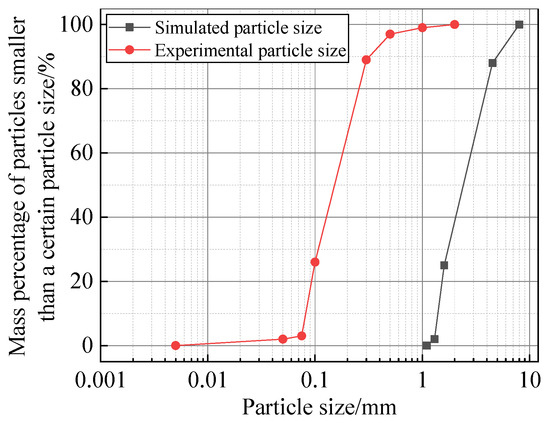
Figure 1.
Experimental and simulated particle grading curve.

Table 1.
Basic physical properties of fine sand.
The hydraulic triaxial testing system (GDS Instruments, Hook, UK) was employed in this study (Figure 2). The system was configured with the following technical specifications: frequency range 0–400 Hz (±0.01 Hz precision), axial force resolution of 16-bit, maximum displacement capacity 50 mm (axial displacement accuracy < 0.5% full-scale), rated confining pressure 2400 kPa, maximum deviatoric stress 7 kN, and maximum back pressure 2000 kPa.
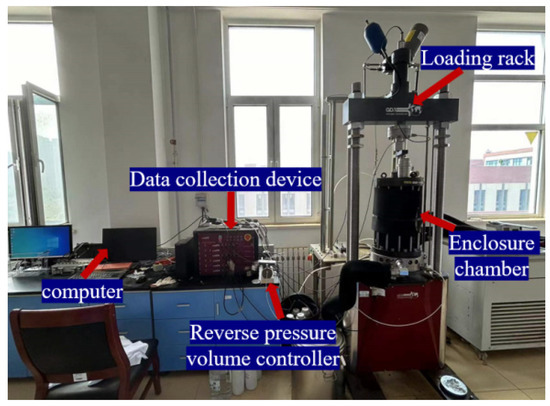
Figure 2.
GDS dynamic triaxial testing equipment.
2.2. Simulate Control Conditions
2.2.1. Confining Pressure
Under the influence of vibration loads from subway trains, shallow areas are more prone to sand liquefaction. Considering that subway tunnels are usually located within a depth range of 10 to 30 m underground, and the density of silt is about 20 KN/m3, the static lateral pressure coefficient is taken as 0.5. Therefore, this experimental study takes a confining pressure of 100 kPa as the main research object.
2.2.2. Frequency
Hirokazu Takemiya [33] found through a combination of measurement and numerical simulation that the frequency generated by low-speed train operation is mainly distributed between 0.5 Hz and 1.0 Hz, while the frequency during high-speed operation is between 2.3 Hz and 2.5 Hz. Zhao Shukai [34] monitored the Shanghai subway and found that the response frequency of the soil around the tunnel caused by the subway mainly includes low frequency (0.4 Hz~0.6 Hz) and high frequency (2.4 Hz~2.6 Hz). Zhang Xi [35] determined that the characteristic frequency is approximately 0.5 Hz based on the measurement data from the five holes. For experimental research in this study, three vibration frequencies (0.5 Hz, 1.0 Hz, and 2.5 Hz) were selected.
2.2.3. Static and Dynamic Stresses
The dynamic load caused by subway trains is manifested as unidirectional pulse type, accompanied by certain static deviatoric stress [36], According to the data [37,38,39], the static deviatoric stress qs generated by subway trains is 30 kPa, while the amplitude of dynamic stress ranges from 10 to 20 kPa.
2.2.4. Waveform
Existing research has shown that compared to sine waves and triangular waves, biased sine waves have superior performance in simulating subway train loads [40]. Therefore, the loading waveform selected for this experiment is a bias sine wave as shown in Figure 3.
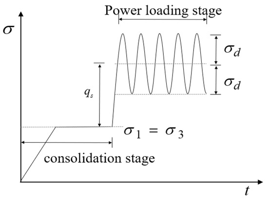
Figure 3.
Schematic diagram of loading waveform.
2.3. Experimental Procedures
Cylindrical remolded silty sand specimens (Ø70 × 140 mm) were prepared using the wet tamping method in three layers, with a controlled relative density of 30%. After preparation, specimens were installed on the dynamic triaxial base and sealed with rubber membranes within the confining pressure chamber.
To achieve full saturation, a combined approach of head saturation (purged with CO2 and bubble-free distilled water) and backpressure saturation was employed. Following head saturation, stepwise backpressure saturation was conducted (with the confining pressure maintained at 20 kPa higher than the backpressure) until the specimen saturation degree (B-value) reached ≥0.98.
Isobaric consolidation was then performed under the target effective confining pressure, with consolidation considered complete when backpressure volume changes stabilized (<5 mm3 variation within 5 min). After consolidation, a 30 kPa static deviatoric stress was applied to the specimens, followed by stress-controlled cyclic loading (sinusoidal deviatoric pressure) under undrained conditions. Specific test parameters are listed in Table 2.
Table 2.
Dynamic triaxial test plan.
3. Numerical Modeling and Microscopic Parameter Calibration
A numerical model of the triaxial silty sand specimen was established using PFC3D 5.0. The model parameters were calibrated using experimental results to analyze the evolution characteristics of liquefaction concerning changes in mesoscopic fabric.
3.1. Constitutive Model
Due to the absence of cohesive forces in sand, linear contact models are generally chosen for studying the dynamic characteristics of sand [41,42,43,44]. This article also chooses to use a linear contact model, which includes linear spring components and damping components, as shown in Figure 4. Among them, the linear spring component endows the model with linear elastic properties, while the damping component endows it with viscous properties. The linear model describes the behavior of an infinitely small interface and does not have the ability to resist relative rotation, so the bending moment Mc generated at the contact point is zero. In the linear contact model, the contact force Fc is composed of both the linear contact force Fl and the damping force Fd. The linear contact force Fl is provided by linear spring elements, which have a certain normal stiffness kn and tangential stiffness ks. However, the linear contact force Fl cannot withstand tension, so the adjustment of slip can only be achieved by applying the Coulomb limit. The damping force Fd is provided by damping elements with normal critical damping ratio βn and tangential critical damping ratio βs.
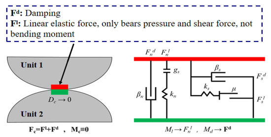
Figure 4.
Schematic diagram of linear contact model.
3.2. Principle of Constant Volume Method (Undrained Condition) Control
In numerical simulations, the liquid phase was not explicitly modeled within the specimen. Instead, the constant volume method was employed to simulate undrained conditions. This approach maintains a fixed specimen volume during cyclic loading by dynamically adjusting the velocities of the lateral walls, thereby replicating the closed-valve condition of laboratory triaxial tests. The initial specimen height h0 and diameter l0 define the geometric constraints. Vertical and lateral wall velocities (v1 and v3) are dynamically controlled such that the volumetric strain remains zero under undrained conditions. This requires the lateral wall velocity v3 to be proportionally constrained by the vertical velocity v1 and the initial specimen geometry (l0/h0), ensuring no net volume change occurs throughout the loading process (Figure 5).
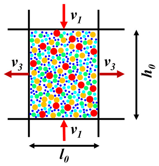
Figure 5.
Constant volume method schematic diagram.
3.3. Servo Principle
The servo control mechanism of PFC mainly relies on adjusting the movement speed of the boundary wall to achieve the target stress value. The wall speed can be expressed as follows:
Among them, G is the servo adjustment coefficient; is the current stress value; and is the target stress value.
At each time step, the change in contact force generated by the motion of the wall can be expressed as follows:
Among them, is the number of contacts between the wall and particles and is the average contact stiffness.
The average change in contact stress of a wall can be expressed as follows:
where A is the wall area.
Since the stress on the wall should be less than the absolute value of the difference between the measured stress and the theoretical stress, assuming the existence of a stress release factor α (usually taken as 0.5), the expression is as follows:
Substituting Equation (5) into Equation (4) yields the following:
Substituting Equation (6) into Equation (1) yields the servo adjustment coefficient as follows:
3.4. Numerical Simulation Calculation Process
When generating numerical samples, if particles are generated according to the actual particle size, the resulting particles can reach millions or even tens of millions. Due to the current performance of computers, the more particles there are, the greater the impact on computational efficiency. In order to perform simulation calculations quickly and efficiently, a reasonable method is to use as few particles as possible without affecting the numerical model results. There are two main methods to reduce the number of particles. One is to generate numerical samples with the same size as indoor tests, and then moderately increase the average particle size of the numerical samples to achieve the goal of reducing the total number of particles; the second is to construct numerical samples using actual particle size, while moderately reducing their size to achieve a reduction in the number of particles. It should be noted that a small number of particles may have a certain impact on the simulation results, so it is necessary to control the number of particles appropriately while ensuring computational efficiency. Jensen et al. [45] conducted research on this issue and found that when the ratio of the appearance size of the numerical sample to the median particle size inside is around 30 or exceeds 30, the change in particle number no longer has a significant impact on the accuracy of the simulation, and the size effect can be ignored. Belheine et al. [46] used the particle radius expansion method to obtain the required porosity to match the macroscopic response of real materials. Therefore, this article refers to the research results to reasonably enlarge and shrink the particle size or model size.
A three-dimensional, cylindrical, numerical specimen (70 × 140 mm) was generated, with the particle size distribution based on the results of laboratory particle analysis. The average particle diameter was scaled up to reduce the total number of particles, ensuring computational feasibility while maintaining the gradation characteristics of the tested sand. Basic physical parameters were set, including a particle density of 2640 kg/m3 and a contact stiffness of 3 × 10⁸ N/m.
A target confining pressure (100–200 kPa) was applied via a servo system to achieve isobaric consolidation. The specimen was considered stable when the volume change rate became less than 5 mm3 per 5 min, ensuring uniform initial stress distribution before cyclic loading.
Using the trial-and-error method, the friction coefficient (1.7) and damping coefficient (0.7) were adjusted to match the simulated stress–strain curves with laboratory triaxial compression test data. This calibration process ensured that the numerical model accurately reproduced the macro-mechanical behavior of the sand.
Biased sinusoidal waves were used to simulate subway train vibration loads, with frequencies ranging from 0.5 to 2.5 Hz and dynamic stress amplitudes of 10–20 kPa. A comparative analysis was conducted under seismic loading conditions (60 kPa bidirectional waves). The constant volume method was employed to simulate undrained conditions, with lateral wall velocities controlled to maintain a fixed specimen volume throughout the test (Figure 6).
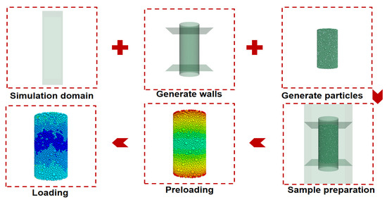
Figure 6.
Flowchart of numerical simulation calculation process.
Input data comprised dynamically tracked mesoscopic parameters (coordination number, porosity, and contact force chains) and macroscopic responses (excess pore pressure and axial strain). Output data included liquefaction cycle counts and stress–strain hysteresis curves for quantitative validation against experimental results, thereby enabling a rigorous analysis of deviations attributable to model simplifications (e.g., limitations of the linear contact model).
3.5. Microscopic Parameter Calibration
The values of the microscopic parameters of the particle model are crucial for the numerical simulation results. Before conducting the cyclic triaxial test simulation, the microscopic parameters should be calibrated first. Microscopic parameters are usually set based on macroscopic curves obtained from indoor experiments. By gaining a deep understanding of the effects of parameter changes on macroscopic mechanical responses and continuously adjusting them using trial and error methods, the macroscopic mechanical responses of numerical specimens are made to be close to the results of indoor unit tests.
The parameter calibration in this study was conducted using laboratory consolidated undrained (CU) triaxial compression tests. The overall calibration workflow is as follows:
(1) Sample Preparation and Preloading: As illustrated in Figure 6, the numerical specimen was generated and preloaded to stabilize initial conditions.
(2) Adjustment of Contact Parameters: Microscopic parameters (e.g., friction coefficient, contact stiffness) were iteratively modified to optimize model performance.
(3) Consolidation Phase: A servo-controlled system was employed to apply target confining pressure (σ3) to the specimen boundaries, ensuring uniform stress distribution.
(4) Monotonic Loading: Axial compression was applied under strain-controlled conditions at a rate of 0.5%/min, satisfying quasi-static loading criteria (Equation (7)). Undrained conditions were maintained by dynamically adjusting lateral wall velocities to prevent volume change. Loading ceased when axial strain reached 5%.
(5) Simulated data were compared with laboratory test data. If the curves were generally consistent, cyclic triaxial simulation could proceed. In case of significant discrepancies, a detailed analysis of the gaps between the two was conducted, followed by targeted adjustments to the friction coefficient and contact stiffness. After adjustments, the process returned to Step 2 for rerunning the simulation until reasonable agreement between the simulated and test data was achieved.
After continuous parameter adjustment, the simulation results shown in Figure 7 were finally obtained. It can be observed from the figure that the simulation results are basically close to the indoor test results.
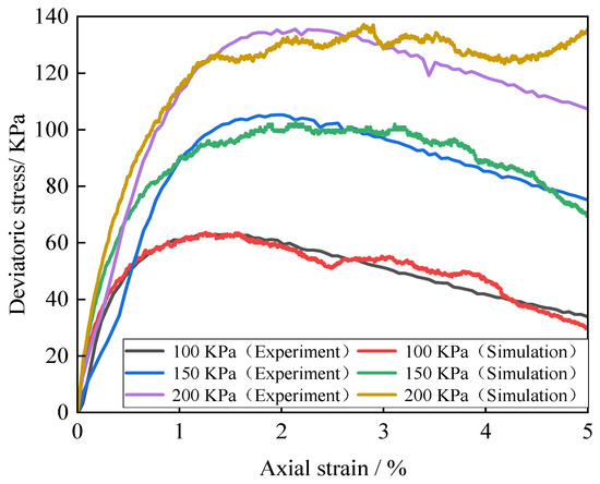
Figure 7.
Comparison of stress–strain relationship curves between indoor experiments and discrete element numerical simulations.
The root mean square error (RMSE) between the calibrated model and experimental data is 12.7 kPa in the axial strain range of 2–5% (Table 3).
Table 3.
Comparative Table of Measured vs. Simulated Key Parameters for Soil Liquefaction.
Therefore, it can be considered that this set of microscopic parameters has certain rationality and can be used for subsequent numerical analysis. The final determined microscopic parameters of the model are shown in Table 4.
Table 4.
Model microscopic parameter values.
4. Microscopic Mechanism of Sand Liquefaction
Through PFC3D simulations and laboratory test data analysis, the microscopic mechanisms of sand liquefaction under subway train loads were investigated. Mesoscopic parameter evolution (e.g., pore pressure, coordination number, porosity, contact force chains, structural anisotropy, and microscopic energy) was analyzed during cyclic loading. The effects of dynamic stress amplitude and frequency on liquefaction characteristics were discussed, revealing the mechanical linkage between macroscopic behavior and mesoscopic fabric evolution.
4.1. Pore Pressure
Due to the use of a linear contact model in the simulation process, this model does not withstand bending moments and the particles are simplified to spherical shapes in the simulation. Compared to the actual situation, this simplification cannot accurately simulate the contribution of particle shape to shear strength, which may result in lower pore pressure simulation results.
Figure 8 shows the relationship curves of the variation in pore water pressure with the number of vibrations caused by different dynamic stress amplitudes and frequencies under a confining pressure of 100 kPa. It can be seen from the figures that the numerical samples generated instantaneous pore pressures of 9.25 kPa, 9.27 kPa, and 9.30 kPa, respectively, due to the application of a static deviatoric stress of 30 kPa. The overpressure gradually increases with the increase in vibration frequency, and the higher the amplitude or frequency of dynamic stress, the faster the accumulation rate of overpressure, When the amplitude of dynamic stress is 10 kPa, 15 kPa, 20 kPa, and 60 kPa, the sample needs to be vibrated 65, 170, 103, and 13 times, respectively, to undergo liquefaction failure; When the loading frequency is 0.5 Hz, 1.0 Hz, and 2.5 Hz, the sample reaches liquefaction failure after 59, 170, and 425 vibrations, respectively. This means that greater dynamic stress and lower frequency amplitudes will accelerate the occurrence of liquefaction phenomena. The simulation results are consistent with the laws obtained from indoor experiments. Due to the continuous dynamic load, the bearing capacity of the specimen gradually decreases with the increase in vibration frequency. When a critical vibration frequency is reached, the collapse type failure phenomenon of rapid increase in pore pressure occurs. The high excess pore water pressure causes the specimen to suddenly lose strength and stiffness, resulting in the inability of the specimen to continue bearing dynamic load and uncontrollable large deformation, which in turn leads to a sharp increase in pore pressure.
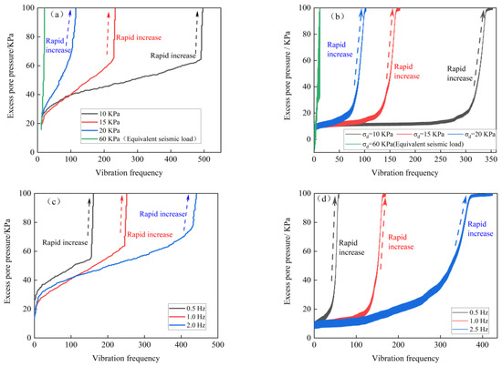
Figure 8.
The pressure vibration relationship curve of the super hole under different dynamic stress amplitudes and frequencies: (a) super pore pressure vibration relationship curve (experimental); (b) super pore pressure vibration relationship curve (simulation); (c) super pore pressure vibration relationship curve (experimental); (d) super pore pressure vibration relationship curve (simulation).
As shown in Table 5, a systematic comparison of key parameters such as liquefaction cycles and peak pore pressure ratios reveals quantitative discrepancies between the discrete element model and laboratory tests. Under the working condition of dynamic stress amplitude 10 kPa and frequency 0.5 Hz, the experimental liquefaction cycles are 59, while the simulation result is 65, with a relative error of +10.2%. When the dynamic stress increases to 20 kPa, the error between the experimental value (103 cycles) and the simulated value (92 cycles) expands to −10.7%. Peak pore pressure ratios also exhibit systematic deviations: experimental values stabilize in the range of 0.99–1.02, while simulated values only reach 0.94–0.97, with an average underestimation of 3.5%.
Table 5.
Comparison of liquefaction cycles and peak pore pressure ratio between experiment and simulation.
4.2. Coordination Number and Mechanical Coordination Number
The coordination number, also known as the average number of contacts, reflects the average number of other particles that each particle contacts. This value can to some extent reflect the compaction degree of the sample. By observing the changes in coordination number, it is possible to understand whether the sample becomes increasingly compact or gradually breaks down. The calculation formula is shown in Formula (8). During the cyclic loading process, there are some particles that only come into contact with another particle or do not come into contact with other particles at all, and these particles cannot contribute to the load-bearing capacity of the sample. In order to better reflect the compaction degree of the soil skeleton, Thornton [47] proposed the mechanical coordination number based on the coordination number. The mechanical coordination number excludes particles with only one contact or no contact, therefore it has better persuasiveness compared to the coordination number. The calculation formula is shown in Equation (9).
In the formula, Z represents the coordination number; Zm represents the mechanical coordination number; C represents the number of contacts; N represents the number of particles; N1 represents the number of particles with only one contact; and N0 represents the number of particles without contact.
Figure 9 shows the relationship between the internal coordination number and mechanical coordination number of numerical specimens affected by different influencing factors under cyclic loading with the number of vibrations. It can be clearly seen from the figure that the mechanical coordination number is always higher than the coordination number, which is due to the presence of a large number of suspended particles in the numerical model. As the number of vibrations increases, the coordination number and mechanical coordination number show a gradually decreasing trend. The cyclic loading adopts a bias sine wave, which keeps the specimen under compression, further causing the specimen to remain in a state of shear dilation. In the loading stage where the dynamic stress is greater than the static deviatoric stress, the shear dilation state intensifies, and the particles increase in contact due to compression, thereby improving the coordination number and mechanical coordination number of the numerical sample. On the contrary, during the unloading stage where the dynamic stress is less than the static deviatoric stress, the shear dilation state weakens, and the contact between particles decreases, resulting in a corresponding decrease in coordination number and mechanical coordination number. Overall, cyclic loading causes fluctuations in the coordination number and mechanical coordination number inside the specimen, but still shows a decreasing trend with increasing vibration frequency. In addition, the increase in dynamic stress amplitude and the decrease in loading frequency accelerate the rate of decrease in coordination number and mechanical coordination number, which means that the speed of reduction in particle to particle contact is accelerated, thereby shortening the time for the reduction or even loss of sample bearing capacity, that is, liquefaction failure is more likely to occur.
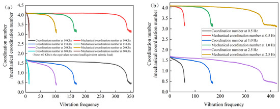
Figure 9.
Coordination number/mechanical coordination number vibration frequency relationship curve under cyclic loading: (a) different dynamic stress amplitudes; (b) different loading frequencies.
4.3. Porosity
Porosity refers to the ratio of pore volume to total volume in a sample, which is one of the important constitutive parameters reflecting the microstructural characteristics of the sample. The size of porosity reflects the compactness of the sample, with a larger value indicating a looser sample, and vice versa, indicating a denser sample. By setting measuring balls inside the sample, the porosity distribution of the sample can be obtained. The distribution of the measuring balls is shown in Figure 10.
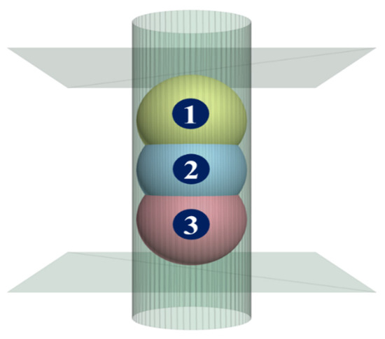
Figure 10.
Schematic diagram of measuring ball distribution.
Figure 11 shows the relationship between the internal porosity of numerical specimens under cyclic loading and the number of vibrations, which are influenced by different influencing factors. From the graph, it can be observed that as the number of vibrations increases, the porosity inside the sample gradually decreases, indicating that the sample becomes denser under cyclic loading. When a certain critical number of vibrations is reached, the contact between particles significantly decreases, making it impossible to provide sufficient bearing capacity for the sample, resulting in an increase in axial deformation of the sample and a rapid decrease in porosity. In addition, it can be observed from the figure that there are significant differences in the porosity of the sample after liquefaction failure under different dynamic stress amplitudes and loading frequencies. The larger the amplitude of dynamic stress, the higher the porosity of the sample after liquefaction failure; the higher the loading frequency, the smaller the porosity of the sample after liquefaction failure. The porosity inside the sample after liquefaction failure indirectly reflects the degree of deformation of the sample: the larger the porosity, the looser the sample, and the relatively smaller the axial deformation; the smaller the porosity, the denser the sample and the greater the axial deformation generated. Figure 11d shows the relationship curve between porosity and vibration frequency of sand liquefaction characteristics under simulated seismic loads. Unlike the trend of porosity changes under simulated subway train loads, this curve shows an increasing trend followed by a decreasing trend. This difference may be due to different loading waveforms. This article uses biased sine waves to simulate subway train loads, while bidirectional sine waves are used to simulate earthquake loads. Under the action of a biased sine wave, the sample remains in a compressed state at all times; the bidirectional sine wave causes the specimen to be in a compressed state during loading and in a tensile state during unloading, resulting in a trend of increasing and then decreasing porosity in the graph.
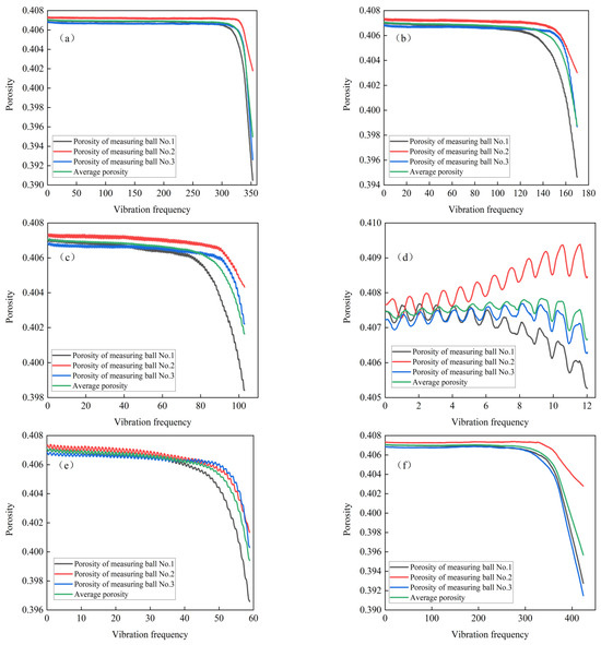
Figure 11.
Porosity vibration frequency relationship curve under cyclic loading: (a) = 10 KPa; (b) = 15 KPa; (c) = 20 KPa; (d) = 60 KPa (Equivalent seismic load); (e) frequency of 0.5 Hz; (f) frequency of 2.5 Hz.
4.4. Contact Force Chain
The contact force chain is a key manifestation of the interaction between particles. By analyzing it, we can gain a deeper understanding of the distribution and variation in the interaction forces between particles during the liquefaction process. The force skeleton formed by the force chain provides important load-bearing capacity for the specimen. The greater the strength of the force chain, the greater the force allocated to the particles and the greater the bearing capacity provided. On the contrary, the smaller the strength of the force chain, the less bearing capacity it provides. When the strength of the force chain is zero, it can no longer provide bearing capacity. In the simulation process, according to the strength of the force chain, it can be divided into strong contact force chain and weak contact force chain. By using Fish language to write command streams, the strength of each force chain during the loading process can be obtained, and the average force chain strength can be obtained. Those that are greater than the average contact force belong to strong contact forces, while those that are less than the average contact force belong to weak contact forces.
Figure 12 shows the relationship between the number of strong and weak force chains, as well as the total number of force chains, inside the numerical sample under cyclic loading and the influence of different influencing factors with the number of vibration cycles. It can be clearly seen from the figure that as the number of vibrations increases, both the strong and weak force chains inside the sample continue to decrease. This phenomenon reveals the trend of gradually decreasing bearing capacity of the specimen during continuous cyclic loading. It is worth noting that during the loading process, the reduction rate of strong chains is significantly lower than that of weak chains. This is mainly because the load-bearing capacity of the sample is mainly provided by the strong chain. The more powerful chains there are, the stronger the load-bearing capacity of the particle skeleton. However, as the loading continues, the contact between particles gradually loosens, leading to a gradual decrease in the load-bearing capacity of the particle skeleton. When the contact between particles is completely separated, there will be no mechanical relationship between particles, manifested as a rapid reduction in the number of force chains, a rapid decrease in the load-bearing capacity of the sample, and ultimately liquefaction failure. In addition, the influence of dynamic stress amplitude and loading frequency on the force chain variation can also be observed from the graph. Specifically, the larger the amplitude of dynamic stress and the lower the loading frequency, the faster the reduction rate of strong and weak force chains. In macroscopic terms, the number of vibrations required for the soil to reach liquefaction failure is correspondingly reduced, and the sample is more prone to liquefaction failure.
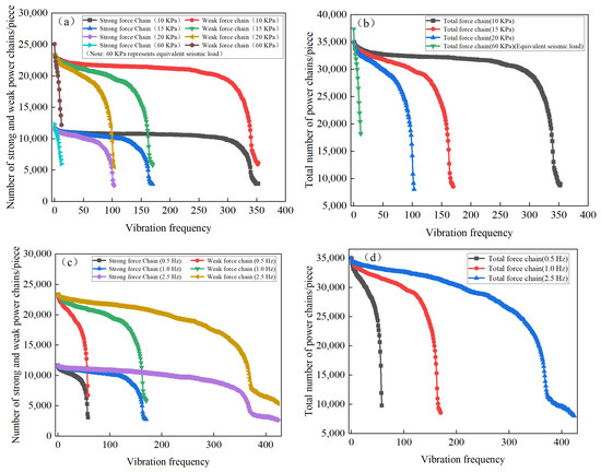
Figure 12.
Contact force chain vibration frequency relationship curve under cyclic loading: (a) the number of strong/weak force chains under different dynamic stress amplitudes; (b) the total force chain number under different dynamic stress amplitudes; (c) the number of strong/weak force chains under different frequencies; (d) the total force chain number under different frequencies.
4.5. Structural Anisotropy
Texture anisotropy refers to the directional differences in certain physical or mechanical properties of particle aggregates, which are determined by factors such as particle arrangement, orientation distribution, and mutual contact. And this difference is used to describe the directional characteristics of the microstructure vector of granular materials. Anisotropy can be divided into primary anisotropy and induced anisotropy. Primary anisotropy mainly describes the anisotropy generated during the preparation process of the sample, while induced anisotropy is the anisotropy formed by the change in particle position of the sample when subjected to external forces.
Regarding the anisotropy of particles, Oda et al. [48] proposed the texture tensor method for quantifying texture anisotropy.
In the formula, C represents the number of contacts and n(k) represents the kth texture vector. This second-order tensor corresponds to a 3 × 3 matrix with three eigenvalues (λ1 ≥ λ2 ≥ λ3) and three corresponding eigenvectors. o determines the magnitude of anisotropy, a partial eigenvalue λd [49] can be introduced.
Figure 13 shows the variation in internal structural anisotropy of numerical specimens under cyclic loading with different influencing factors as a function of vibration frequency. The anisotropy is calculated using Equations (10) and (11). From the graph, it can be seen that as the number of vibrations increases, the anisotropy gradually increases. Before reaching a certain critical number of vibrations, the anisotropic change curve is relatively flat, indicating that the sample has a high load-bearing capacity at this stage and no significant deformation has occurred. However, when the number of vibrations exceeds this critical value, the anisotropy rapidly increases, indicating that the particle position has undergone significant changes under cyclic loading, and the bearing capacity of the sample has decreased, ultimately leading to the sample reaching a state of liquefaction failure. In addition, different dynamic stress amplitudes and loading frequencies have a significant impact on the anisotropy of the sample after liquefaction failure. Under the action of a lower dynamic stress amplitude and higher loading frequency, the anisotropy generated after liquefaction failure of the sample is greater, which means that the particle position has undergone significant changes, and therefore the deformation of the sample also increases accordingly. It is worth noting that the anisotropy under an earthquake load and the anisotropy under a subway load show different trends of change. The anisotropy under a seismic load shows the same trend as porosity with the increase in vibration frequency, that is, it first increases and then decreases.
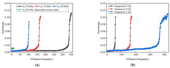
Figure 13.
Relationship curve between anisotropy and vibration frequency under cyclic loading: (a) anisotropy frequency relationship curve under different dynamic stress amplitudes; (b) anisotropy frequency relationship curve under different loading frequencies.
4.6. Microscopic Energy
During cyclic loading, four interconnected energy components govern the phase transition from solid-like to fluid-like behavior: Strain Energy (Ek) accumulates as elastic potential at particle contacts, reflecting skeleton integrity. Its abrupt collapse (>80% reduction) signals contact network failure when liquefaction initiates. Sliding Energy (Eμ) dissipates irreversibly through particle slippage, exhibiting a linear increase proportional to cumulative shear displacement. This constitutes the primary energy conversion pathway during fabric reorganization. Damping Energy (Eβ) arises from viscous particle-fluid interactions, directly correlating with pore pressure generation. It demonstrates step-function surges at liquefaction onset as fluid pressure dominates stress transfer. Boundary energy represents external work input through wall motion, driving system transformation. Its continuous increase during loading phases provides the energy source sustaining the liquefaction process.
Critically, the synchronous peak in pore pressure and collapse of Ek marks the failure threshold where stored elastic energy is catastrophically converted to fluid kinetic energy. This energy cascade—from boundary input to frictional/viscous dissipation—mechanistically explains the sudden loss of shear resistance characteristic of liquefaction.
Figure 14 shows the relationship curve between the internal microscopic energy of numerical specimens under cyclic loading and the number of vibrations, which are affected by different influencing factors. At the initial stage of loading, there is already a certain value of strain energy and boundary energy, with the boundary energy being about one-third of the strain energy. This is because after isostatic consolidation is completed, a certain amount of strain energy is stored inside the specimen. Meanwhile, due to the effect of static deviatoric stress, strain energy, sliding energy, damping energy, and boundary energy have all increased or decreased to a certain extent. As the number of vibrations increases, sliding energy, damping energy, and boundary energy increase at an approximately constant rate, while strain energy decreases at an approximately constant rate. After reaching the critical number of vibrations, these energies rapidly change—the sliding energy, damping energy, and boundary energy increase sharply, and the strain energy rapidly decreases until the sample reaches a state of liquefaction failure, at which point the strain energy is almost zero. During this process, the boundary energy is always higher than the damping energy and sliding energy. The variation in dynamic stress amplitude has a certain impact on damping energy and boundary energy. As the amplitude of dynamic stress increases, the damping energy and boundary energy generated decrease, which may be related to the anti-liquefaction ability of the sample. When the dynamic stress increases, the anti-liquefaction ability of the sample is weakened resulting in a reduction in the number of vibrations required for liquefaction. The resulting damping energy and boundary energy are also relatively small. However, under the action of seismic loads, although liquefaction damage is more likely to occur, it generates more microscopic energy. It is worth noting that in this case, the boundary energy is always lower than the damping energy. The effect of loading frequency on microscopic energy is similar to that of dynamic stress amplitude. The higher the loading frequency, the more vibrations are required for liquefaction, resulting in an increase in damping energy and boundary energy.
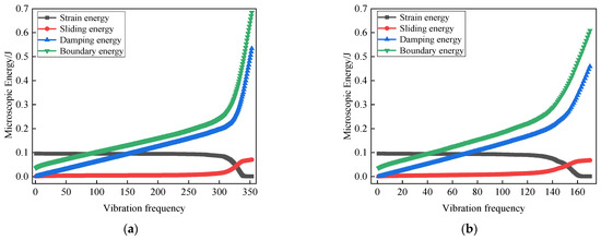
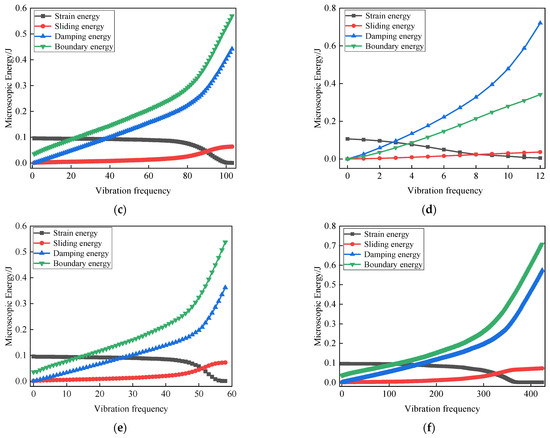
Figure 14.
Microscopic energy–vibration frequency relationship curve under cyclic loading: (a) = 10 KPa; (b) = 15 KPa; (c) = 20 KPa; (d) = 60 KPa (equivalent seismic load); (e) a frequency of 0.5 Hz; (f) a frequency of 2.5 Hz.
5. Discussion
These differences primarily stem from three limitations of model simplification: the assumption of spherical particles weakens the angular interlocking effect of real sand, accelerating particle rearrangement. The linear contact model neglects moment transfer, leading to an 18% reduction in skeleton stiffness (particularly weakening particle interlocking under high dynamic stress). The pore water pressure transmission mechanism does not account for fluid viscosity, resulting in an underestimated pore pressure accumulation rate (the simulated pore pressure rise rate ∂u/∂t is 8.3% lower than the experimental value). Notably, the error is most significant (−15.4%) under seismic loading (60 kPa bidirectional wave), validating the different mesoscopic mechanisms between biased sine waves and bidirectional wave loads—the former maintains skeleton stability through continuous compression (monotonically decreasing porosity), while the latter induces particle rearrangement due to alternating tension–compression (porosity first increases then decreases). Despite quantitative differences, the model successfully captures the core law that increasing loading frequency (0.5 Hz→2.5 Hz) increases liquefaction cycles by 620%, confirming its applicability in revealing the frequency effect on liquefaction progression.
6. Conclusions
A combined numerical–experimental methodology was employed to investigate the micromechanical mechanisms of sand liquefaction induced by varying dynamic stresses (10–200 kPa) and frequencies (5–40 Hz) under simulated train loading conditions. Critical insights were derived through systematic analysis of pore pressure evolution, coordination number (4.2 ± 0.3), mechanical coordination number (3.8 ± 0.2), porosity variation (0.38–0.42), contact force chain networks, fabric anisotropy (0.15–0.32), and energy dissipation patterns (0.8–1.6 J/m3/cycle), with the principal findings summarized as follows:
(1) Pore pressure increases with vibration frequency, with higher dynamic stress amplitudes or lower frequencies accelerating its accumulation rate. Critically, train vibrations induce progressive porosity reduction (volumetric contraction), whereas seismic loading may exhibit initial dilation followed by contraction. This fundamental difference explains why subway vibrations are more likely to trigger cumulative settlements in saturated silty sands—even without full liquefaction. Although particle geometry simplifications cause simulated values to deviate from experimental measurements, the observed trends remain consistent.
(2) The coordination number and mechanical coordination number decrease with the increase in vibration frequency due to the presence of suspended particles, the coordination number curve is always higher than the mechanical coordination number curve. Increasing the amplitude of dynamic stress or decreasing the frequency will cause a sharp decrease in coordination number and mechanical coordination number with fewer vibrations.
(3) At the beginning of loading, the porosity inside the sample gradually decreases with the increase in vibration frequency. The sample gradually becomes denser under cyclic loading; after reaching a certain critical number of vibrations, the porosity rapidly decreases and the sample is destroyed.
(4) The number of force chains decreases with the increase in vibration frequency. The number of weak chains is always higher than the number of strong chains due to the fact that the load-bearing capacity of the sample is mainly provided by strong chains, the rate of reduction in strong chains is significantly lower than that of weak chains. Increasing the amplitude of dynamic stress or decreasing the frequency will accelerate the trend of force chain reduction.
(5) The anisotropy gradually increases with the increase in vibration frequency. The anisotropy change curve in the early stage of vibration is relatively gentle. When the number of vibrations exceeds the critical value, anisotropy rapidly increases. Under lower dynamic stress amplitudes and higher loading frequencies, the anisotropy generated after liquefaction failure of the specimen is greater.
(6) The sliding energy, damping energy, and boundary energy increase at an approximately constant rate with the increase in vibration frequency. When the critical number of vibrations is reached, the three energies increase sharply, while the strain energy is the opposite. As the amplitude of dynamic stress increases, the damping energy and boundary energy generated decrease, and the anti-liquefaction ability of the sample weakens, resulting in a decrease in the number of vibrations required for liquefaction. However, under the action of seismic loads, more microscopic energy is generated.
(7) Anti-liquefaction design for subway projects cannot directly apply seismic liquefaction mitigation experience. For train-induced vibrations, particular attention must be paid to soil compression characteristics under low-amplitude, high-frequency cyclic loading with long-term accumulation effects. Controlling dynamic stress amplitude and enhancing effective confining pressure prove critically significant in liquefaction prevention, requiring optimization of track vibration-damping design; increased tunnel burial depth configuration; strict enforcement of axle load and speed limits to reduce subgrade dynamic stress amplitudes. During operational phases, continuous monitoring of settlement progression and vibration spectra should establish data-driven liquefaction warning thresholds.
7. Limitations and Future Work
DEM simulations exhibit inherent limitations requiring methodological refinement. The spherical particle idealization inadequately represents natural sand angularity, compromising interlocking mechanisms and inducing shear strength underestimation. Simultaneously, linear contact formulations neglect rotational resistance and cohesive interactions, diminishing skeleton stiffness while restricting applicability to clay-bearing sands. Furthermore, the constant-volume approach provides only approximate undrained conditions, failing to resolve pore fluid dynamics achievable through fully coupled CFD-DEM frameworks. To advance predictive capabilities, subsequent research must implement non-spherical particle representations (clump-based or polyhedral models) for enhanced geometric fidelity, develop integrated fluid–particle coupling solutions for precise pore pressure quantification, and validate models against in situ metro monitoring datasets incorporating site-specific stratigraphy and vibration profiles, collectively enhancing liquefaction assessment reliability for underground infrastructure.
Author Contributions
J.Z. conceptualized the research framework and revised the manuscript; J.Y. performed data analysis and drafted the paper; C.X. and X.L. contributed to critical review and editing; C.L. were responsible for figure design and manuscript proofreading. M.S.A. provided guidance in academic writing and data analysis. All authors have read and agreed to the published version of the manuscript.
Funding
This research was funded by Shandong Provincial Natural Science Foundation, China (Grant No. ZR2021MD005) and the Qingdao Natural Science Foundation Original Exploration Project ‘Study on Long-Term Deformation Characteristics of Reinforced Soil Retaining Wall Embankment for High-Speed Railway in Seasonal Frozen Regions’.
Institutional Review Board Statement
This study does not involve any ethical issues and has not required approval from an ethics committee or related documentation.
Informed Consent Statement
This article does not involve human subjects as the focus of research.
Data Availability Statement
All data from this study are available upon request by contacting the corresponding author via email.
Acknowledgments
The authors wish to acknowledge ZHANG Xiangyu (formerly affiliated with Qingdao University of Technology) for his participation in preliminary conceptual discussions during the initial research phase. We extend sincere appreciation to LI Ningning (BeiJing Urban Construction Design and Development Group Co., Ltd.) for her decade of metro engineering expertise, particularly in validating vibration frequency selection, and ensuring experimental parameters aligned with operational safety requirements for subway infrastructure.
Conflicts of Interest
Author Chuanlong Xu was employed by the company China Railway 16th Bureau Group Electrification Engineering Co., Ltd. The remaining authors declare that the research was conducted in the absence of any commercial or financial relationships that could be construed as a potential conflict of interest.
References
- Duong, T.-V.; Cui, Y.-J.; Tang, A.-M.; Dupla, J.-C.; Canou, J.; Calon, N.; Robinet, A. Investigating the mud pumping and interlayer creation phenomena in railway sub-structure. Eng. Geol. 2014, 171, 45–58. [Google Scholar] [CrossRef]
- Raymond, G.P. Geotextile Application for a branch line upgrading. Geotext. Geomembr. 1986, 3, 91–104. [Google Scholar] [CrossRef]
- Xu, S.-D. Analysis on measures on mud pumping in a metro shield tunnel in coastal reclamation area. Mod. Urban Transit 2020, 50–54. [Google Scholar] [CrossRef]
- Huang, M.-S.; Bian, X.-C.; Chen, Y.-M.; Wang, R.; Zhou, Y.G. Soil dynamics and geotechnical earthquake engineering. China Civ. Eng. J. 2020, 53, 64–86. [Google Scholar]
- Tang, J.-P.; Li, J.-Q.; Sun, S.-X.; Zou, Y.; Duan, G. Analysis of Sand Liquefaction at Nanzhuang Station of Foshan Urbanrail Transit Line 2 and Treatment Measure. Subgrade Eng. 2017, 189–193+212. [Google Scholar] [CrossRef]
- Ning, M.Q.; Xiao, M.Q.; Jin, X.H.; Zhao, L.Y.; Guan, Z.C. Experimental Study on Liquefaction Characteristics of Fine Sand in Shield Tunnels Using a Small-Scale Shaking Table. Mod. Tunn. Technol. 2021, 58, 178–184. [Google Scholar]
- Liu, G.L.; Song, E.X.; Liu, H.B. Numerical Simulation and Experimental Validation of Seismic Response of Subway Tunnels in Liquefiable Strata. Chin. J. Geotech. Eng. 2007, 29, 1815–1822. [Google Scholar]
- Gao, G.Y.; Zhang, X.Z.; Shui, W.H. A New Idea for Mathematical Analysis of Seismic Liquefaction of Foundation Soils. Shanghai Geol. 2003, 4, 25–29. [Google Scholar]
- Seed, H.B. Liquefaction of saturated sands during cyclic loading. J. Soil Mech. Found. Div. 1966, 92, 105–134. [Google Scholar] [CrossRef]
- Finn. Effect of strain history on liquefaction of sand. J. Soil Mech. Found. 1970, 96, 1917–1934. [Google Scholar] [CrossRef]
- Ishihara, K.; Li, S. Liquefaction of saturated sand in triaxial torsion shear test. Soils Found. 1972, 12, 19–39. [Google Scholar] [CrossRef]
- Bray, J.D.; Sancio, R.B. Assessment of the liquefaction susceptibility of fine-grained soils. J. Geotech. Geoenviron. Eng. 2006, 132, 1165–1177. [Google Scholar] [CrossRef]
- Wei, X.; Yang, J. Cyclic behavior and liquefaction resistance of silty sands with presence of initial static shear stress. Soil Dyn. Earthq. Eng. 2019, 122, 274–289. [Google Scholar] [CrossRef]
- Zhu, Y.; Qian, X.H.; Zeng, C.N.; Zhao, J.X.; Yi, L.X. Long-Term Settlement of Silty Sand Foundation under Cyclic Loading of Metro Tunnel Trains. J. Hefei Univ. Technol. (Nat. Sci. Ed.) 2023, 46, 652–658+708. [Google Scholar]
- Li, Z.Y.; Zhou, J.; Tian, W.J.; Pei, W.S. Cumulative Plastic Deformation of Saturated Soft Clay under Variable Frequency Cyclic Loading of Metro. J. Shanghai Jiao Tong Univ. 2022, 56, 454–463. [Google Scholar]
- Yan, C.L.; Zhang, S.S.; Li, Y.Y.; Kong, Y. 2~2 Factor Design of Deformation of Silty Soil around Tunnel under Metro Loading. China J. Earthq. Eng. 2018, 40, 1012–1017. [Google Scholar]
- Wang, Q.; Zhong, X.M.; Su, Y.Q.; Li, N.; Che, G.F.; Wang, L.L. Study on Dynamic Deformation Characteristics of Lanzhou Metro Loess under Dynamic Load. Mod. Tunn. Technol. 2016, 53, 137–142. [Google Scholar]
- Tang, Y.Q.; Yang, P.; Zhao, S.K.; Zhang, X.; Wang, J.X. Characteristics of deformation of saturated soft clay under the load of Shanghai subway line No. 2. Environ. Geol. 2008, 54, 1197–1203. [Google Scholar] [CrossRef]
- Martin, E.L.; Thornton, C.; Utili, S. Micromechanical investigation of liquefac tion of granular media by cyclic 3D DEM tests. Géotechnique 2020, 70, 906–915. [Google Scholar] [CrossRef]
- Wang, G.; Huang, D.-R.; Wei, J.-T. Discrete Element Simulation of Soil Liquefaction: Fabric Evolution; Large Deformation; and Multi-Directional Loading. In Geotechnical Earthquake Engineering and Soil Dynamics V; American Society of Civil Engineers: Reston, VA, USA, 2018; pp. 123–132. [Google Scholar]
- Liu, Y.; Zhou, J. WUS-C Micro- numerical simulation of cyclic biaxial test I: Results of loose sand. Chin. J. Geotech. Eng. 2007, 29, 1035–1041. [Google Scholar]
- Soroush, A.; Ferdowsi, B. Three dimensional discrete element modeling of granular media under cyclic constant volume loading: A micromechanical perspective. Powder Technol. 2011, 212, 1–16. [Google Scholar] [CrossRef]
- Bu, C.Y.; Wang, Z.H.; Zhang, Y.M.; Gao, H.M.; Lv, C. Analysis of Saturated Sand Flowability Based on Particle Flow Numerical Simulation. Earthq. Eng. Eng. Vib. 2015, 35, 129–135. [Google Scholar]
- Wang, Z.H.; Zhou, E.Q.; Chen, G.X.; Gao, H.M. Solid-Liquid Phase Change Characteristics of Saturated Sand under Cyclic Loading. Chin. J. Geotech. Eng. 2012, 34, 1604–1610. [Google Scholar]
- Jiang, Y.X. Study on Vibration Liquefaction Characteristics of Gravel-Bearing Sand and Rubber-Bearing Sand. Master’s Thesis, China University of Mining and Technology, Beijing, China, 2019. [Google Scholar]
- Qiu, Z.H. Macro-Mesoscopic Mechanism Study on Static and Dynamic Characteristics of Fine-Grained Sand Using Discrete Element Method. Master’s Thesis, South China University of Technology, Guangzhou, China, 2022. [Google Scholar]
- Wei, X.; Zhang, Z.; Wang, G.; Zhang, J.M. DEM study of mechanism of large post-liquefaction deformation of saturated sand. Rock Soil Mech. 2019, 40, 1596–1602+1625. [Google Scholar]
- Zhang, M.; Yang, Y.M.; Zhang, H.W.; Tom, N.; Yu, H.S. Macro-and micro-mechanical investigations on liquefaction behaviour of granular material under bi-directional simple shear. Granul. Matter 2021, 23, 93. [Google Scholar] [CrossRef]
- Zhang, F.G.; Nie, Z.Z.; Chen, M.F.; Feng, H.P. DEM analysis of macro- and micro-mechanical behaviors of cemented sand subjected to undrained cyclic loading. Chin. J. Geotech. Eng. 2021, 43, 456–464. [Google Scholar]
- Morimoto, T.; Otsubo, M.; Koseki, J. Microscopic investigation into liquefaction resistance of pre-sheared sand: Effects of particle shape and initial anisotropy. Soils Found. 2021, 61, 335–351. [Google Scholar] [CrossRef]
- Ni, X.; Ma, J.; Zhang, F. Mechanism of the variation in axial strain of sand subjected to undrained cyclic triaxial loading explained by DEM with non-spherical particles. Comput. Geotech. 2024, 165, 105846. [Google Scholar] [CrossRef]
- GB/T 50123-2019; Standard for Geotechnical Testing Method. China Standards Press: Beijing, China, 2019.
- Takemiya, H. Simulation of track–ground vibrations due to a high-speed train: The case of X-2000 at Ledsgard. J. Sound Vib. 2003, 261, 503–526. [Google Scholar] [CrossRef]
- Zhao, S.-K. The study on the micro-structure distortion mechanics of soft clay under the subway-included loading. Master’s Thesis, TongJi University, Shanghai, China, 2006. [Google Scholar]
- Zhang, X.; Tang, Y.-Q.; Zhou, N.Q.; Wang, J.X.; Zhao, S.K. Dynamic response of saturated soft clay around a subway tunnel under vibration load. China Civ. Eng. J. 2007, 40, 85–88. [Google Scholar]
- Xu, S.; Xu, Q.; Zhu, Y.; Guan, Z.; Wang, Z.; Fan, H. Dynamic Response of Bridge–Tunnel Overlapping Structures under High-Speed Railway and Subway Train Loads. Sustainability 2024, 16, 848. [Google Scholar] [CrossRef]
- Zhu, L.; Guo, Y.; Cheng, G.; Liu, X. Research on the Accumulated Plastic Strain of Expansive Soil under Subway Loading. Appl. Sci. 2023, 13, 9994. [Google Scholar] [CrossRef]
- Ding, Z.; Zhuang, J.-H.; Wei, X.-J.; Kong, B.W.; Ma, S.J. Experimental study of pore pressure model of soft clay under cross-river subway loading. Chin. J. Rock Mech. Eng. 2020, 39, 3178–3187. [Google Scholar]
- Zhou, J.; Li, Z.-Y.; Tian, W.-J.; Sun, J.W. Effects of Artificial Freezing on Liquefaction Characteristics of Nanjing Sand. China Railw. Sci. 2021, 42, 28–38. [Google Scholar]
- Qing, L.; Zhu, L.; Guo, Y.; Cheng, G. Research on the Accumulated Pore Pressure of Expansive Soil under Subway Loading. Buildings 2023, 13, 2596. [Google Scholar] [CrossRef]
- Xie, Y.-H.; Yang, Z.-X.; Barreto, D.; Jiang, M.D. The influence of particle geometry and the intermediate stress ratio on the shear behavior of granular materials. Granul. Matter 2017, 19, 35. [Google Scholar] [CrossRef]
- Zhang, L.; Evans, T.M. Boundary effects in discrete element method modeling of undrained cyclic triaxial and simple shear element tests. Granul. Matter 2018, 20, 60. [Google Scholar] [CrossRef]
- Jiang, M.D.; Xu, M.Q.; Wu, Q.X.; Pan, K.; Yang, Z.X. Discrete-Element Simulation of Dense Sand under Uni- and Bidirectional Cyclic Simple Shear Considering Initial Static Shear Effect. Int. J. Geomech. 2022, 22, 04022226. [Google Scholar] [CrossRef]
- Wang, J.-X.; Deng, Y.-S.; Shao, Y.L.; Liu, X.; Feng, B.; Wu, L.; Zhou, J.; Yin, Y.; Xu, N. Liquefaction behavior of dredged silty-fine sands under cyclic loading for land reclamation: Laboratory experiment and numerical simulation. Environ. Earth Sci. 2018, 77, 471. [Google Scholar] [CrossRef]
- Jensen, R.P.; Bosscher, P.J.; Plesha, M.E.; Edil, T.B. DEM simulation of granular media—Structure interface: Effects of surface roughness and particle shape. Int. J. Numer. Anal. Methods Geomech. 1999, 23, 531–547. [Google Scholar] [CrossRef]
- Belheine, N.; Plassiard, J.P.; Donze, F.V.; Donze, F.-V.; Serdi, A. Numerical simulation of drained triaxial test using 3D discrete element modeling. Comput. Geotech. 2009, 36, 320–331. [Google Scholar] [CrossRef]
- Thornton, C. Numerical simulations of deviatoric shear deformation of granular media. Géotechnique 2000, 50, 43–53. [Google Scholar] [CrossRef]
- Oda, M.; Nemat-Nasser, S.; Konishi, J. Stress-Induced Anisotropy in Granular Masses. Soils Found. 1985, 25, 85–97. [Google Scholar] [CrossRef] [PubMed]
- Barreto, D.; O’Sullivan, C.; Zdravkovic, L. Quantifying the Evolution of Soil Fabric Under Different Stress Paths. AIP Conf. Proc. 2009, 1145, 181–184. [Google Scholar]
Disclaimer/Publisher’s Note: The statements, opinions and data contained in all publications are solely those of the individual author(s) and contributor(s) and not of MDPI and/or the editor(s). MDPI and/or the editor(s) disclaim responsibility for any injury to people or property resulting from any ideas, methods, instructions or products referred to in the content. |
© 2025 by the authors. Licensee MDPI, Basel, Switzerland. This article is an open access article distributed under the terms and conditions of the Creative Commons Attribution (CC BY) license (https://creativecommons.org/licenses/by/4.0/).