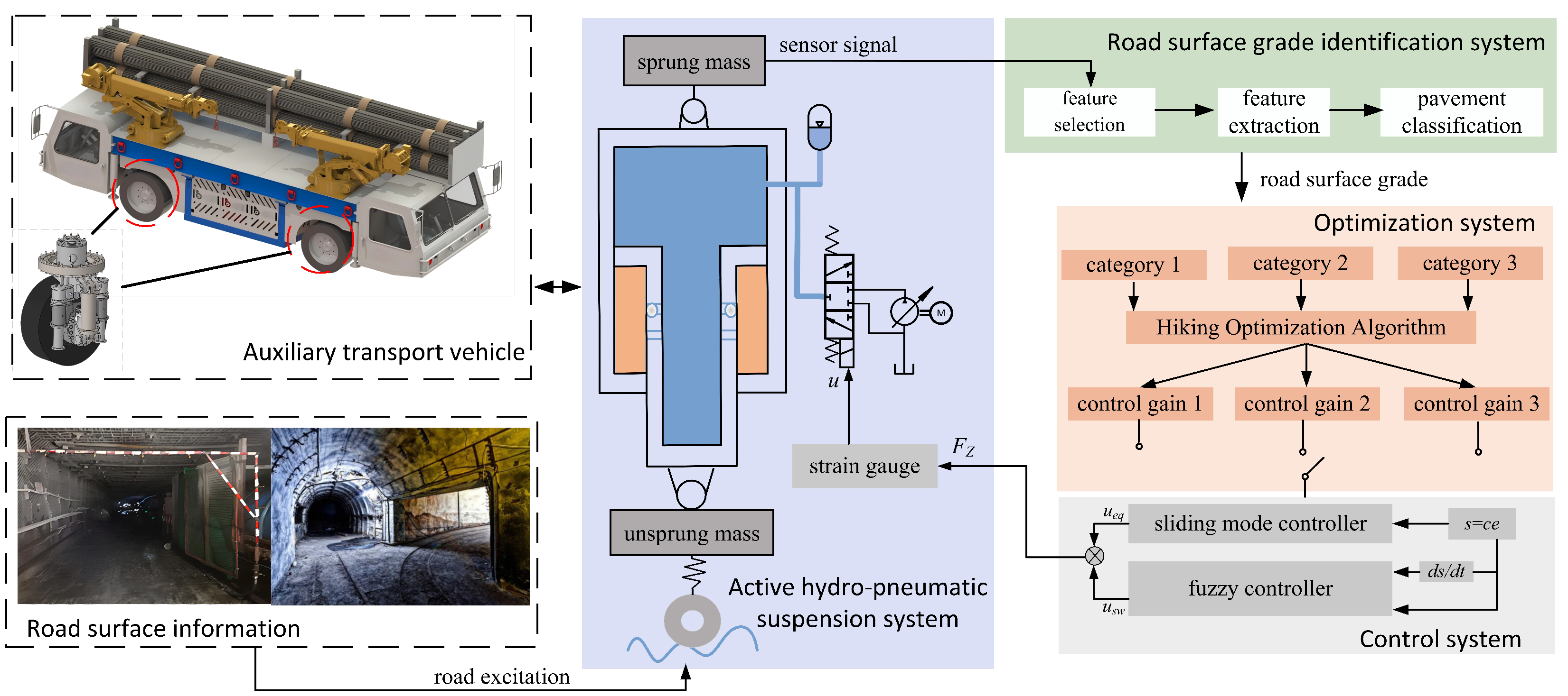
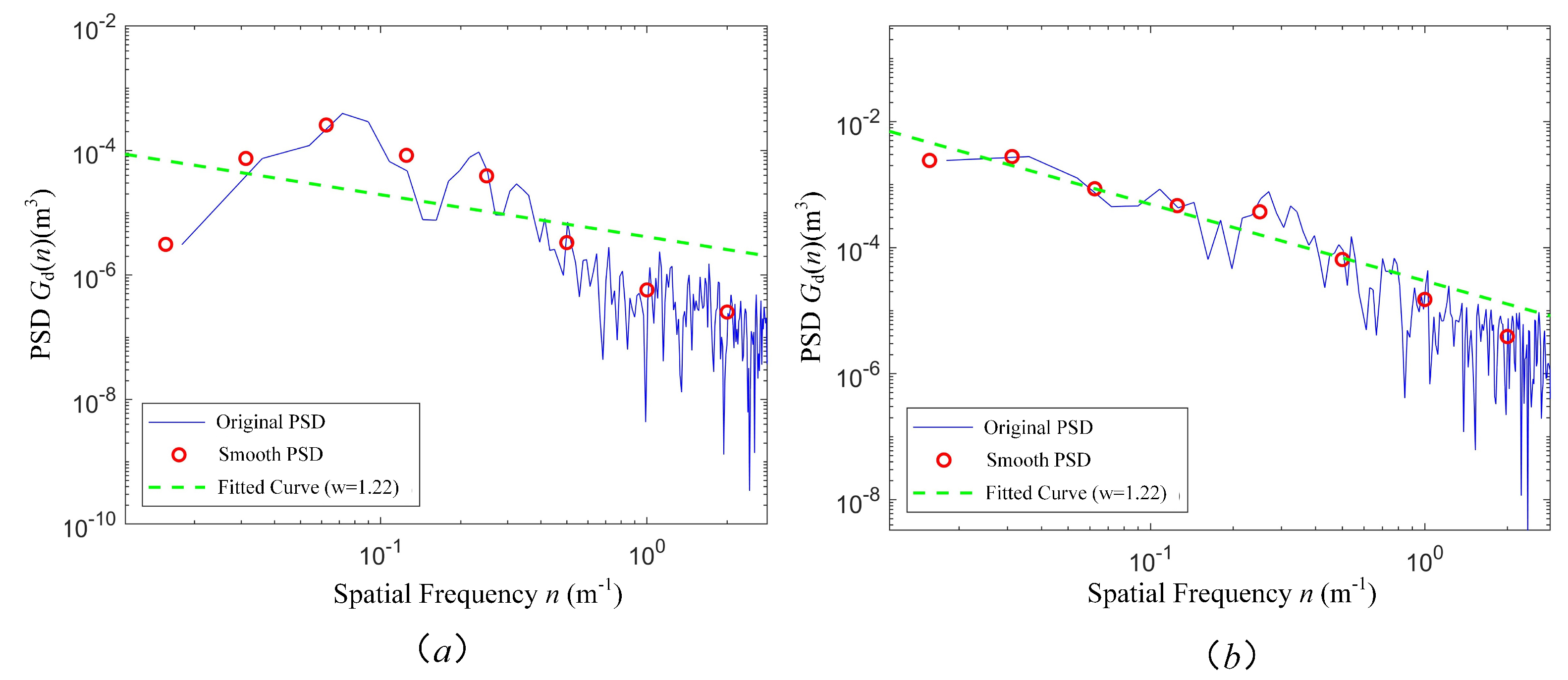
This paper conducted an experimental study based on a real vehicle’s road surface data collection to assess the efficacy of the suggested classification model. The experimental vehicle was operated under various typical road conditions. This study classifies road surfaces into three categories: Type 1: A- and B-grade roads, which are smooth and have low vibration, where the primary goal is to adjust the suspension to optimize the ride comfort. Type 2: C- and D-grade roads, where the conditions are average, with bumps and unevenness, requiring the suspension to enhance the traction and ensure stability. Type 3: E- and F-grade roads, which have poor conditions, with strong vibrations and potential safety risks, requiring the balanced adjustment of both the ride comfort and stability. The controller’s design and parameter optimization framework are shown in
Figure 5.
4.1. Sliding-Mode Control
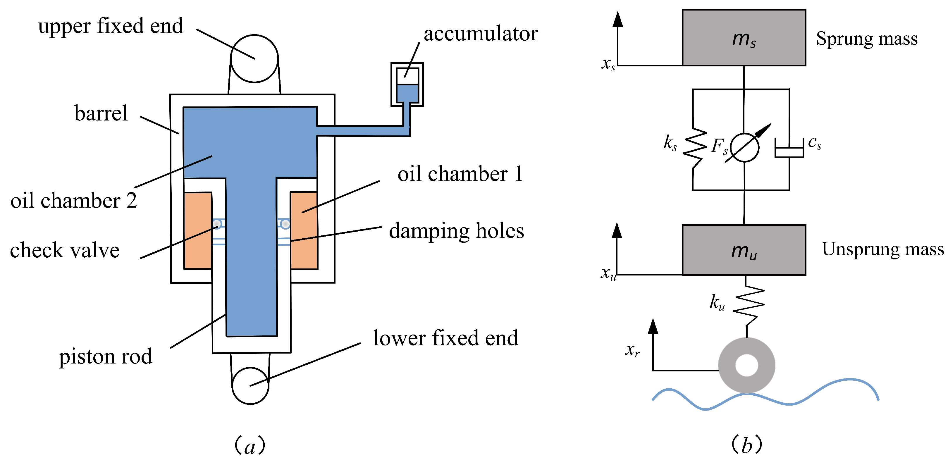
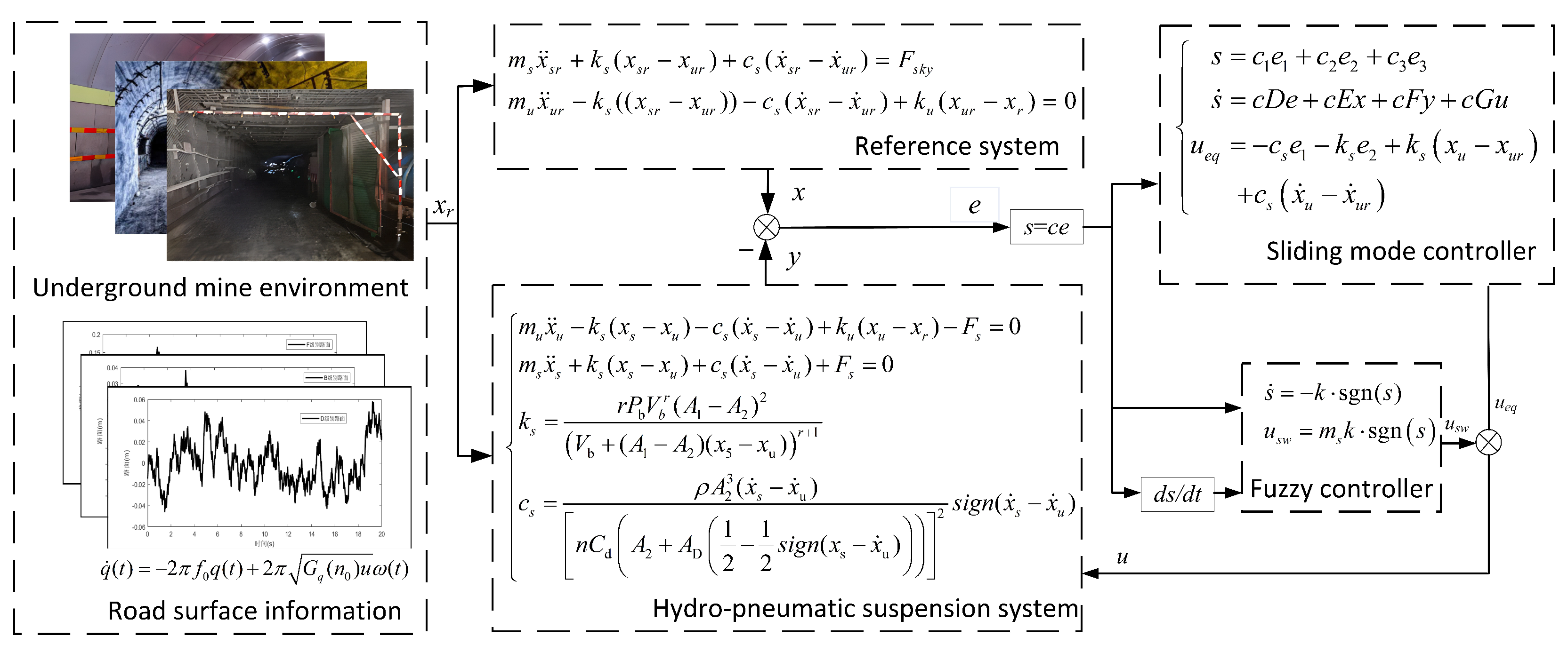
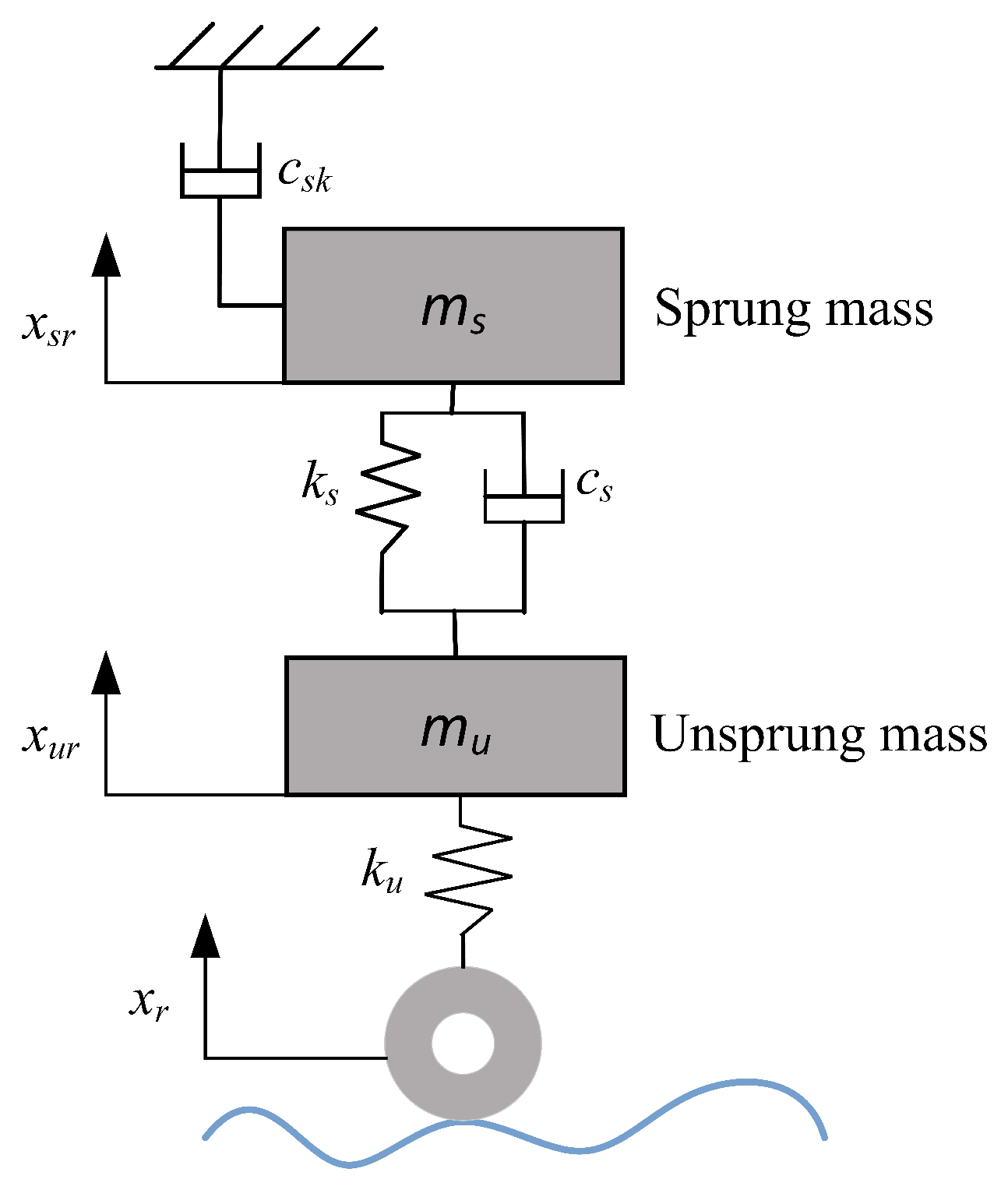
Before diving into the design of the Sliding-Mode Controller (SMC), it is essential to lay the groundwork by setting up a reference model. In this study, an ideal Skyhook model [
21] is shown in
Figure 6. The core idea behind sliding-mode control is to craft a controlled force that effectively guides the spring-loaded mass in the two-degree-of-freedom system to mirror the behavior of its counterpart in the reference Skyhook model. The reference model’s differential equation is as follows:
The equation describing the reference model reads as follows:
where
represents the vehicle body’s reference displacement,
denotes the wheel’s reference displacement,
is the Skyhook damping coefficient, and
is the Skyhook damping force,
.
The reference state vector is defined as follows:
Based on the body mass displacement’s integral error, the displacement error, and the velocity error of the vehicle model with a two-degree-of-freedom active suspension, as well as the suspension model with ideal Skyhook damping, the error vector (
e) for the hydropneumatic suspension system is expressed as follows:
The derivative of the error:
The error state equation:
where system matrices D, E, F, and G:
The sliding surface (s) is expressed as an error-weighted sum as follows:
where the
c values are coefficient matrices selected based on the pole placement. All the states of the sliding mode’s dynamics must exhibit satisfactory transient performance and maintain asymptotic stability throughout the reaching phase to the switching manifold. The characteristic equation of the sliding mode, denoted as
, is as follows:
To ensure the minimal oscillation when the closed-loop system possesses conjugate complex poles in the left half-plane, the following design specifications are imposed: an overshoot of , a peak time of , a natural frequency of rad/s, and a damping ratio of . These yield the system’s eigenvalues (), consequently determining the control gain vector .
The derivative of the sliding surface is as follows:
The speed of the convergence is selected as follows:
where
is a gain parameter.
The sliding-mode control’s output force is as follows:
A Lyapunov function is defined as follows:
To differentiate it and substitute it, we can obtain:
Using Lyapunov stability theory, shows that the control system is stable.
4.2. Fuzzy-Logic-Based Sliding-Mode Controller’s Design
The SMC is widely used in complex systems due to its robustness and disturbance rejection properties, but high-frequency switching can lead to chattering, which negatively affects the system’s stability. To address this issue, a Fuzzy Control (FC) is combined with the SMC, forming a Fuzzy Sliding-Mode Controller (FSMC), which effectively reduces chattering while maintaining the robustness of the SMC [
22].
In designing the FC, input and output variables need to be determined first. In this section, the sliding surface (
s) and
are used as inputs, and the
k values (required for the sliding mode’s control) are used as outputs, and they are defined as follows:
Let the fuzzy-logic-based domains for
s,
, and
k be defined as follows:
The input and output membership function curves are illustrated in
Figure 7a–c, while
Table 5 outlines the fuzzy-logic-based control rules. By applying fuzzy-logic-based inference, the system evaluates the input variables’ membership degrees alongside the rule-based control logic to determine the appropriate output, and the fuzzy-logic-based control output is determined [
23]. The defuzzification process is then carried out using the centroid method to obtain the precise control value. After this, the fuzzy-logic-based control rule’s surface, shown in
Figure 7d, is generated using Matlab’s Fuzzy Logic Toolbox.
Through multiple simulation experiments, the basic domain of the controller is , , and , with quantification factors and gains , , and calculated.
4.3. Controller’s Parameter Optimization
Based on the driving road conditions and the results of the road surface grade identification, the three types of road surfaces correspond to the ride comfort mode, stability mode, and comprehensive adjustment mode, with different suspension controller parameter settings for each mode. Traditional manual parameter selection is inefficient and prone to errors and lacks adaptability. Therefore, this paper uses the Hiking Optimization Algorithm (HOA) to optimize the FSMC parameters.
The HOA [
24] simulates human decision-making behavior during hiking, adjusting strategies based on the natural environment, paths, and difficulty. As a nature-inspired metaheuristic algorithm, the HOA is mainly used for function optimization and global optimization problems. It can perform a global search across a broad solution space, avoiding local optima, thus improving the optimization effect of the controller. By adaptively adjusting the search strategy, the HOA enhances the controller’s adaptability and robustness and is particularly suitable for nonlinear and uncertain problems, aligning with the needs of the FSMC.
The core process of the HOA applied in this study consists of three key phases. First, the population is randomly initialized, and the fitness is assessed within the parameter boundaries. Second, during the iterative optimization process, (1) the current optimal and worst individuals are identified; (2) the base velocity component is computed based on random slope generation; (3) a new velocity vector is synthesized by combining the base velocity, the learning term toward the optimal individual, and the term away from the worst individual (the intensity of the learning is regulated by a random sweep factor); (4) the individual positions are updated, and boundary constraints are processed; and (5) a greedy strategy is used to decide whether or not to accept the new solution. Finally, the optimal solution and its fitness are recorded at each iteration. The algorithm achieves the global optimal search of parameters through a slope-driven velocity mechanism and an elite learning strategy of sweep factor regulation.
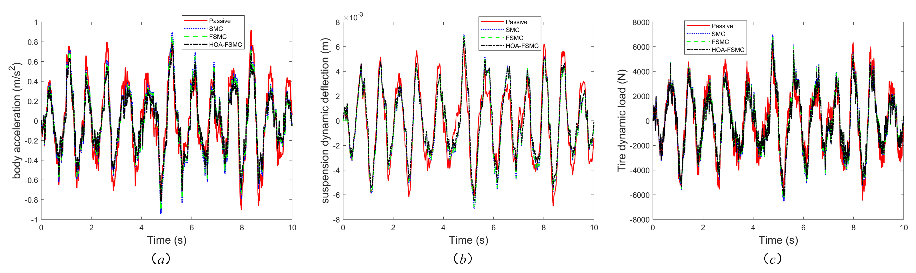
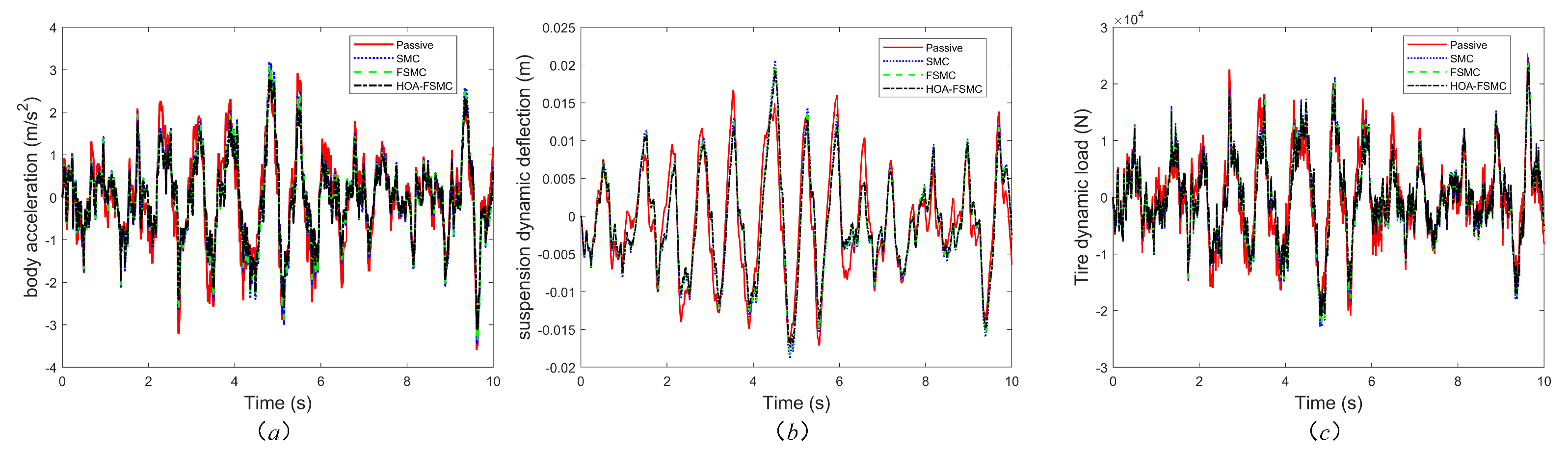
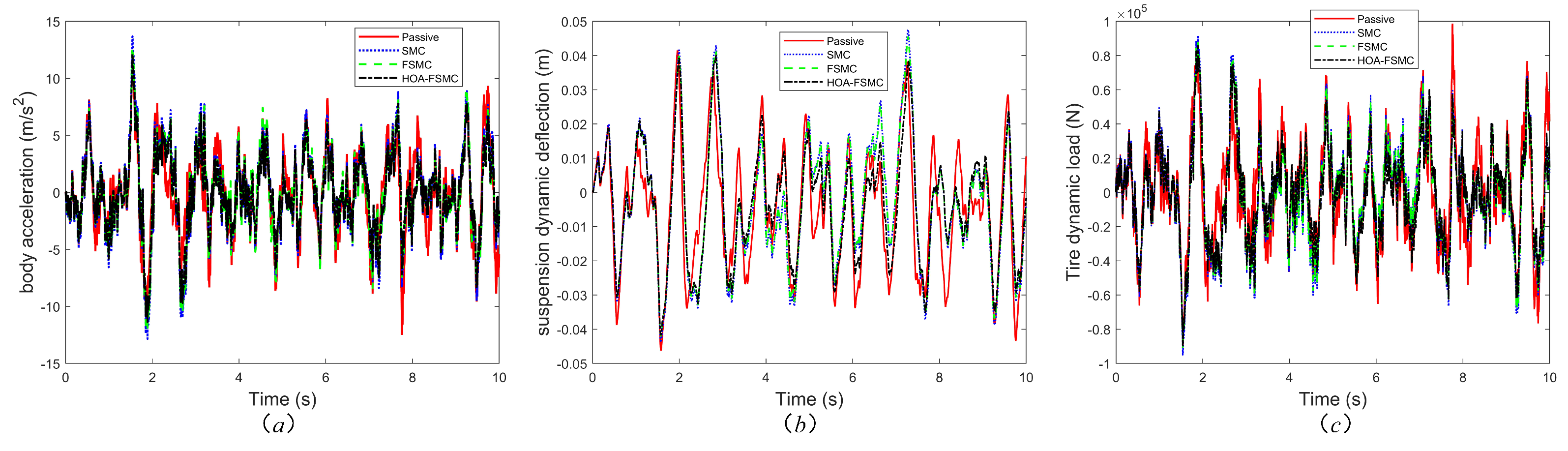
The HOA optimizes the FSMC’s parameters for each type of road surface. Given the complexity of the road surface types, B-, D-, and F-grade road surfaces are selected for optimization. The selected parameters for the SMC include , , , and two scaling factors ( and ), along with a quantization factor (). The optimization goal function is the weighted sum of the following three objectives: the sprung mass’s acceleration, the suspension’s dynamic deflection, and the tires’ dynamic load.
The optimization model is expressed as follows:
where
a and
represent the body’s accelerations for the HOA-FSMC and passive suspension, respectively.
and
represent the suspension’s dynamic deflections for the HOA-FSMC and passive suspension, respectively.
and
represent the tires’ dynamic load for the HOA-FSMC and passive suspension, respectively, and
,
, and
represent the weights for the sprung mass’s acceleration, the suspension’s dynamic deflection, and the tires’ dynamic load, respectively.
The optimization weights for the different road surfaces are shown in
Table 6. During underground mine operations, the auxiliary transport vehicle’s suspension controller should dynamically adjust the weighting coefficients of the performance metrics based on road roughness levels. Under favorable road conditions, it should focus on comfort and give more weight to the spring load’s acceleration. Under moderate road conditions, it should take into account comfort and durability, appropriately reduce the weight of the spring load’s acceleration, and increase the weight of the tires’ dynamic load. Under severe road conditions, it should give priority to guarantee the safety of the suspension and the tires’ grounding performance to improve the comprehensive performance. This adaptive weighting strategy enables context-aware optimization, where the controller emphasizes the most critical performance indices under varying terrain conditions, thereby enhancing the holistic system performance.
The initial values of the parameters to be optimized, as well as the upper and lower limits of the search range, are shown in
Table 7. The search range fluctuates by 50% around the initial values, with the overall search range being 100% of the initial value.
For each road surface type, the HOA algorithm is set with a population size of 20 and a maximum number of iterations of 100. During the optimization process, the fitness of the B-grade (Type 1), D-grade (Type 2), and F-grade (Type 3) road surface conditions decreases, and the controller’s performance improves. After 100 iterations, the system converges for all three road surface types. Finally, the optimized control parameters for the various road surface grades are shown in
Table 8.


 ,
, 


