Towards a Digital Twin Approach for Structural Stiffness Assessment: A Case Study on the Cho’ponota L1 Bridge

Abstract

In this study, a series of comprehensive experimental tests were conducted to assess the impact of permanent displacements observed during the construction of the Cho’ponota L1 Bridge in Uzbekistan and to evaluate the bridge’s structural suitability for service. The investigation included Operational Modal Analysis and static and dynamic vehicular load tests, conducted using two trucks with different weights under varying loading scenarios and speeds. A total of 28 static and 24 dynamic load cases were tested across the bridge’s four spans. Displacement measurements were acquired using geodetic instruments during the static tests, while acceleration data were recorded during dynamic tests using high-sensitivity accelerometers, from which Dynamic Amplification Factors were calculated. The results indicated that all displacement values remained within permissible safety limits, and no visible damage or cracking was detected. Beyond conventional analysis, the study proposed a test-assisted digital twin framework in which high-fidelity field data were integrated into a finite-element model. The initial numerical model was calibrated using modal properties obtained from OMA, and discrepancies were minimized through iterative updates to material parameters, especially concrete stiffness. The resulting validated digital twin accurately reflects the bridge’s current structural condition and can be used for future predictive simulations and performance-based evaluations. The findings underscore the effectiveness of combining non-destructive testing with digital twin methodology in diagnosing structural behavior and offer a replicable model for assessing bridges experiencing construction-related anomalies.

1. Introduction

Bridges play a critical role in the sustainability of economic, social, and cultural life as fundamental components of transportation networks. These essential structures are known to experience performance losses over time due to various natural disasters (e.g., earthquakes and floods) or human-induced factors (e.g., overloading and construction defects). Identifying and evaluating such damages is crucial for ensuring the long-term safe usage of bridges. This assessment is typically performed using various methods, including static and dynamic loading tests, numerical analyses via the finite-element method, visual inspections, and various damage detection techniques. However, many of these methods provide limited information or pose a risk of causing damage to the structure. At this point, Non-Destructive Testing (NDT) methods emerge as a more effective and practical solution for assessing bridge performance. These methods enable the reliable evaluation of structural performance by determining dynamic characteristics without causing any harm to the structure.

Highways and bridges are regarded as significant indicators of a country’s level of development. Developed countries utilize computer-aided Bridge Management Systems (BMSs) to identify and resolve issues related to their existing bridges. By employing these BMSs, countries conduct a general condition assessment of their bridges based on scoring systems tailored to their national criteria [1]. While visual inspection forms the basis of these scoring systems, each country also incorporates its own advanced scoring criteria. For instance, in the United States, photographs of bridge components are taken and digitized in a computer environment to calculate crack dimensions [2]. In Japan, the scoring process has been automated, moving away from human dependency through the use of a fuzzy logic-based artificial neural network program [3]. Developed countries use this general condition information for various purposes, such as prioritizing maintenance and repair work, planning future costs, predicting the future condition of a bridge, and estimating its remaining service life. This approach enables highways to be used continuously and safely without interruption. For example, a 1991 study in Japan revealed that 18,000 of 60,000 bridges required strengthening [4]. Similarly, in the United States, the total cost of maintaining and repairing 540,000 bridges was estimated to be approximately USD 200 billion [5].

Bridges are fundamental components of national and international transportation networks, not only in developed countries but also in developing nations and many regions worldwide. These structures play a critical role in ensuring the sustainability of economic, social, and cultural life. However, in many areas, the structural condition of bridges is typically addressed only when issues arise during their service life. Inspections conducted in response to unplanned problems often lead to disruptions in transportation, unforeseen costs, and significant time losses. Preventing such situations is essential to ensure the safe, efficient, and long-lasting use of bridges. In particular, reliable, effective, and cost-efficient methods for condition assessment have become a priority research area in engineering to avoid transportation disruptions and enable rapid interventions.

Traditional assessment methods, such as visual inspection, often fail to provide sufficient information and are subject to personal interpretation. Procedures like core sampling, on the other hand, pose a risk of causing physical damage to the structure. In contrast, non-destructive testing (NDT) methods offer a modern alternative for evaluating the performance of bridges. These methods enable the direct acquisition of crucial information, such as dynamic characteristics (e.g., natural frequencies, mode shapes, and damping ratios), without causing harm to the structure. In the literature, various studies have focused on identifying potential damages using NDT methods, including Operational Modal Analysis (OMA) tests [6,7,8,9,10,11,12,13], fiber optic sensors [14,15,16,17,18,19,20,21], laser-based measurement systems [22,23,24,25], acoustic emission methods [26,27,28], ultrasonic testing [29,30,31,32,33], and computer vision, artificial intelligence, machine learning, and deep-learning-based approaches [34,35,36,37,38]. These methods facilitate both the reliable analysis of the current condition and the identification of the root causes of structural issues. Non-destructive methods are particularly advantageous for bridges where structural alterations are undesirable and for the preservation of historically significant bridges [39,40,41].

The Digital Twin (DT) paradigm has become a cornerstone in modern infrastructure management by enabling virtual representations of physical systems, continuously updated through sensor integration, computational modeling, and intelligent analysis. The concept, initially developed by NASA and formalized by Grieves and Vickers (2017) [42], has since evolved into a multidisciplinary framework applied in various domains such as manufacturing, medicine, and infrastructure [43,44,45,46]. A DT typically comprises three fundamental elements: the physical asset, its virtual counterpart, and the data connection linking the two [42]. Depending on data connectivity and interaction, DTs are often classified as Digital Models, Digital Shadows, or full Digital Twins, while Predictive DTs incorporate AI-driven feedback loops for simulation and control [47,48]. In recent years, the digital twin paradigm has been increasingly adopted for civil infrastructure systems, particularly for bridges, due to its potential for enabling data-driven diagnostics, predictive maintenance, and lifecycle management [49,50,51,52,53]. The integration of sensor fusion techniques, such as InSAR, computer vision, and machine-learning algorithms, has further enhanced the ability of digital twins to capture complex structural behaviors [53]. Additionally, model-updating approaches continue to play a central role in ensuring the fidelity for stiffness and damage assessment purposes [54,55]. Building upon these advancements, this study proposes a test-assisted digital twin methodology specifically tailored for post-construction stiffness verification of concrete bridges.

The service life of a bridge is directly related to the environmental impacts and the repetitive traffic loads it experiences. During the design phase, anticipated vehicular loads are considered, and these load conditions are incorporated into the design calculations. However, in some cases, a bridge may fail to exhibit sufficient resistance to these planned loading conditions after it becomes operational, resulting in stress and displacement values exceeding acceptable limits. This situation can significantly reduce the intended service life of the bridge. To prevent such issues, bridges are subjected to comprehensive static and dynamic load tests after construction and before being opened for service. These tests are of great importance to verify whether the stress, displacement, and acceleration values measured on the bridge elements remain within specified limits. It is critical to carefully plan these testing and loading procedures to avoid causing damage to the structure. There are documented cases of bridge collapses during the load testing phase [56]. However, when conducted according to proper loading protocols, these tests serve as effective tools to confirm the compliance of a bridge with its design specifications and to reliably evaluate its performance. In these tests, two types of vehicular load testing are performed: static and dynamic. In static load testing, trucks are positioned at predetermined locations on the bridge, and sensors installed on the structure record data such as accelerations, displacements, and stresses. In dynamic load testing, the dynamic effects created by a truck passing over the bridge at specific speeds are measured using sensors placed on the structure. Increases in the truck’s weight and speed during the test result in increased stress and displacement values [57]. For this reason, load tests are conducted with vehicles of varying weights and speeds, designed to be compatible with the bridge’s design. The vehicles used in these tests typically weigh more than 20 tons and move at speeds ranging from 10 to 80 km/h [58,59]. The frequencies, mode shapes, stresses, and displacements obtained from static and dynamic load tests are used to calibrate the finite-element model of the structure. In this way, the actual finite-element model representing the bridge is obtained based on real bridge data [60,61,62,63,64,65,66,67,68,69]. In addition, stiffness separation methods have been proposed to enhance damage identification and reduce computational cost in large-scale truss structures by focusing on partial-model-based updating strategies [70,71]. Although such approaches target different structural systems and objectives, they reflect the growing trend of incorporating model refinement techniques to improve structural diagnostics.

In civil and structural engineering, DTs offer a framework for monitoring, diagnostics, and lifecycle assessment of bridges and other infrastructures [72,73]. Studies have demonstrated the use of computer vision, sensor fusion, and InSAR techniques for twin-driven monitoring [74], and data-driven models such as DCNN-LSTM for simulating thermal displacements in large-span bridges [75]. Semantically enriched models such as BIM-integrated DTs have also enhanced asset interoperability and documentation in smart cities and cultural heritage domains [76,77]. Common architectural frameworks, including ISO 23247-2 and RAMI 4.0, define structural guidelines for integrating these technologies [78,79].

The primary objective of this study is to assess whether the Cho’ponota L1 Bridge has undergone a loss of stiffness due to excessive deflection observed after the application of dead loads and to evaluate the structural usability under service conditions. To this end, a comprehensive field campaign was conducted, including visual inspections, vehicular static and dynamic load testing, and ambient vibration measurements via the OMA method. These procedures were implemented to determine the bridge’s dynamic characteristics—namely, its natural frequencies and mode shapes—and to identify the sources of the observed structural response anomalies. The resulting test data, including frequency content, displacement values, stress distributions, and mode shapes, were used to calibrate a finite-element model of the bridge. While these methods follow established structural assessment protocols, the present study advances the methodology by framing the calibrated FE model as a test-assisted Digital Twin. This concept represents a novel intermediary approach between traditional one-off assessments and fully integrated, continuously updated digital twin systems. Despite the increasing interest in digital twin applications in civil infrastructure, there is a clear research gap regarding field-validated, limited-duration digital twin implementations, particularly in scenarios where full-time monitoring is infeasible. By integrating high-fidelity test data into a dynamic and diagnostically interpretable numerical model, this study provides a replicable digital twin framework for post-construction verification and stiffness assessment in existing bridges. The following sections detail the testing procedures, sensor layout, and data processing stages that form the basis of test-assisted digital twin structural performance evaluation. Compared to fully integrated predictive digital twin frameworks that rely on continuous real-time data streams and AI-driven feedback mechanisms [47], the methodology presented in this study offers a test-assisted digital twin approach that operates based on discrete, high-fidelity experimental datasets. This allows for effective calibration and validation of the structural model even in the absence of long-term sensor deployments. The proposed framework thus provides a practical and cost-effective solution for post-construction structural assessment, particularly for infrastructure systems where real-time data integration may not be feasible due to logistical or financial constraints.

2. Testing the Cho’ponota L1 Bridge

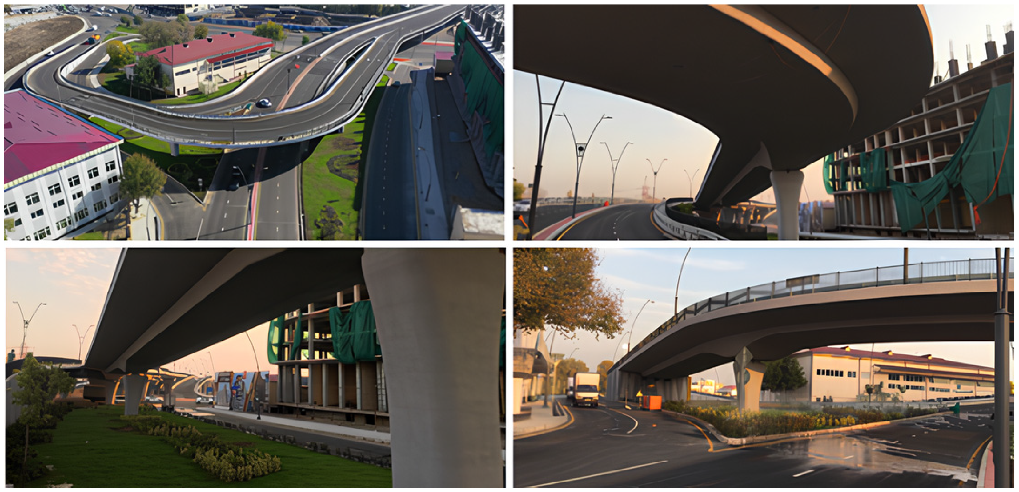
2.1. Description of the Cho’ponota L1 Bridge

The Cho’ponota L1 Bridge is an infrastructure project of engineering and aesthetic significance, located approximately 390 m above sea level in the Sergeli district of Tashkent, the capital of Uzbekistan. Completed in 2021, the bridge serves as a critical structure, enhancing the regional transportation network. The necessity for its construction and its regional impact were conceptualized in a feasibility study developed by Allegro Develop Project Institute, while the technical details were designed by Kalyon Transportation Engineering and Consultancy Co. The construction process was conducted by Grand Road Tashkent and Durable Beton. The general appearance of the bridge is illustrated in Figure 1.

The Cho’ponota L1 Bridge is a 156-m-long structure designed as a four-span, post-tensioned reinforced concrete bridge. Its span arrangement consists of two spans of 33 m and two spans of 45 m. The deck width ranges between 10.00 m and 13.25 m, while the sectional height varies from 1 to 2 m. The bridge is built on a piled foundation system, and the material properties of its structural components are provided in

Table 1. Material properties of Cho’ponota L1 Bridge (Structural Analysis Report, 2020).

No.	Element	Material Class
1	Pile	C25/30
2	Foundation	C25/30
3	Column	C30/35
4	Slab	C50/60

[80].

The design process was based on the American AASHTO LRFD [81] standards and employed a four-stage construction methodology. The prestressed reinforced concrete system used in the bridge facilitates the safe and economical crossing of long spans while effectively bearing the traffic loads in the region.

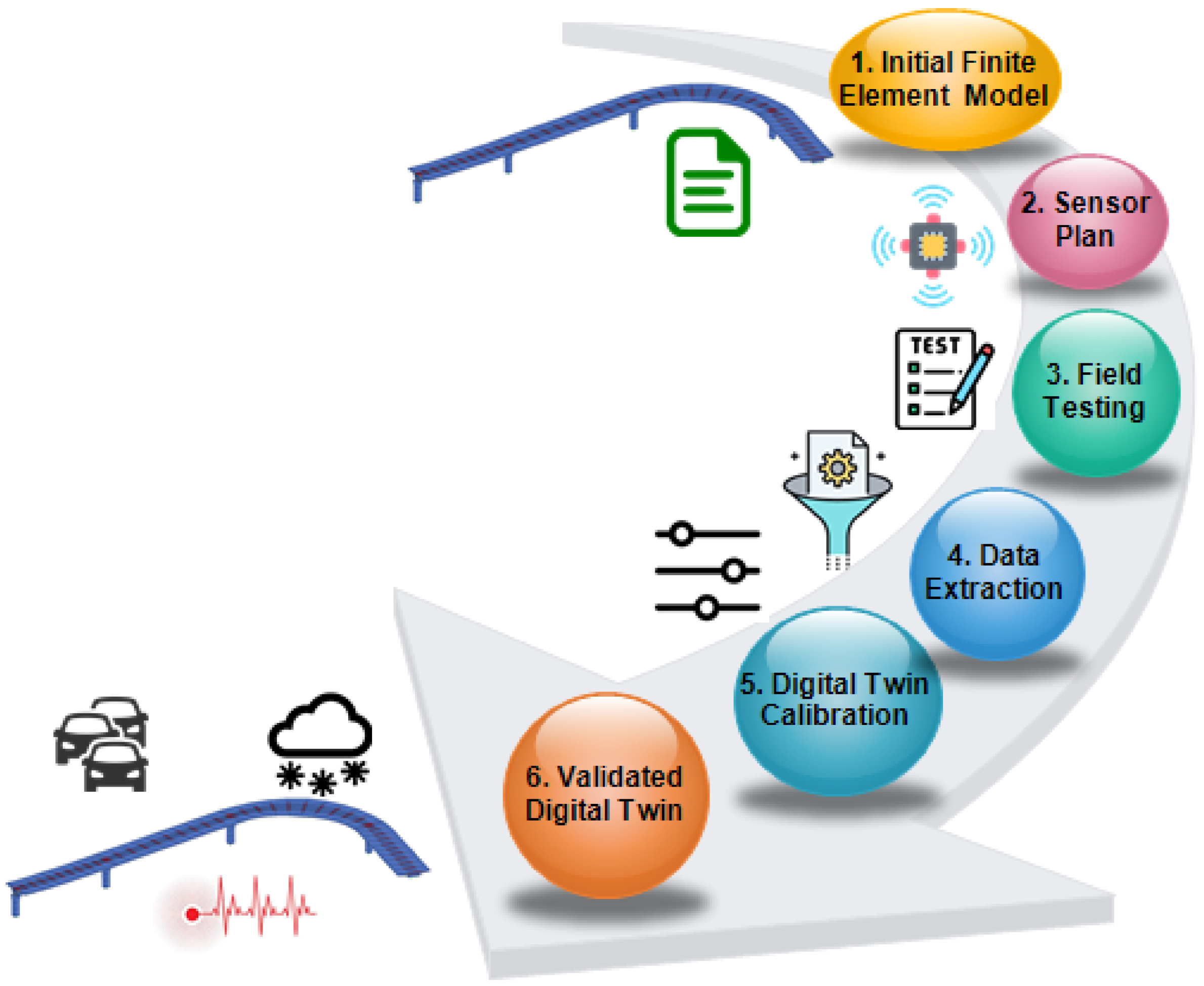
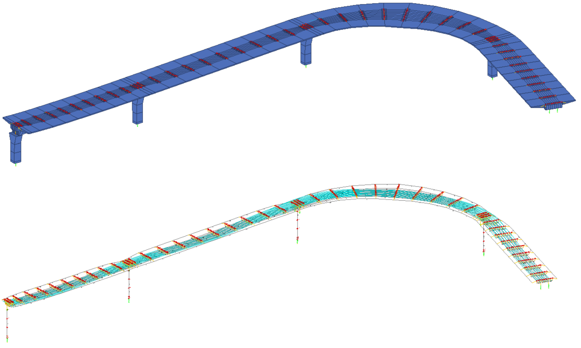
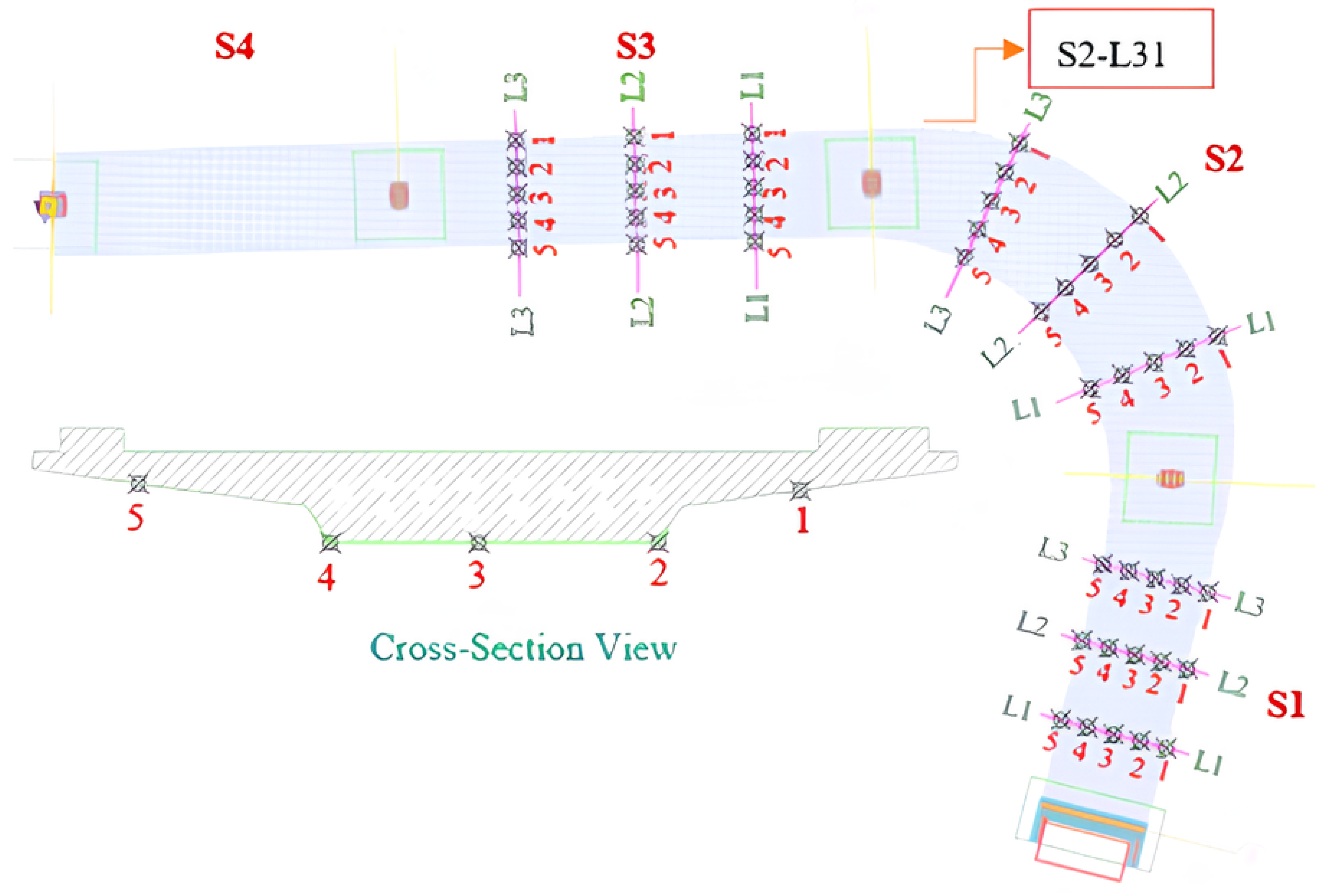
2.2. Digital Twin Construction: Experimental Setup, Field Instrumentation, and Modeling Interface

The test-assisted digital twin framework developed for the Cho’ponota L1 Bridge is structured around a hybrid methodology that combines a physics-based numerical model with targeted experimental data. The process begins with the development of an initial finite-element model constructed using as-built drawings and project specifications. This preliminary model establishes the geometric and mechanical foundation of the virtual structure. To optimize the experimental design, a modal analysis is performed, identifying the critical mode shapes and response zones. These findings inform the sensor placement strategy, ensuring that field measurements capture the most structurally informative locations.

Prior to field testing, a preliminary modal analysis was conducted using the initial finite-element model developed from as-built drawings and project specifications. This analysis provided estimates of the structure’s natural frequencies and mode shapes, which were used to optimize the sensor layout by identifying antinodal positions for critical bending modes. The resulting sensor configuration ensured effective capture of modal responses during OMA. Additionally, the preliminary model outputs guided the planning of static and dynamic load test scenarios, allowing for the safe excitation of the bridge while maximizing the structural response data required for subsequent model calibration. Subsequently, field testing is conducted using static and dynamic vehicular load tests, in addition to ambient vibration measurements through OMA. The collected raw data are processed to extract structural response characteristics such as natural frequencies, mode shapes, and displacement time histories. These experimental results serve as the benchmark for the calibration of the finite-element model. Through an iterative validation process, model parameters—particularly concrete stiffness and boundary conditions—are adjusted to minimize discrepancies between simulated and measured responses. This calibration step transforms the numerical model into a digital twin that reflects the actual behavior of the bridge.

Although the digital twin constructed in this study does not operate with continuous data flow, its validation through high-fidelity test data allows it to be used for realistic simulations under both current and design-level loading conditions. The final digital twin provides a reliable platform for condition assessment, structural diagnostics, and predictive simulations, even in the absence of long-term monitoring infrastructure. This approach shows a practical and scalable pathway for integrating digital twin technologies into civil infrastructure projects, particularly where logistical or financial constraints preclude real-time data integration. An overview of this test-assisted digital twin workflow is illustrated in Figure 2.

The finite element model of the Cho’ponota L1 Bridge was developed using RM Bridge software based on as-built drawings and design documentation. The bridge deck, piers, and pile foundations were modeled using 3D frame (beam) elements capable of capturing flexural, torsional, axial, and shear behavior. Post-tension effects were incorporated through equivalent section properties reflecting the increased stiffness of the post-tension concrete components. Rigid link elements were used to represent the connections between the superstructure and substructure. Initial material properties were assigned according to project specifications: C50/60 concrete for the deck, C30/35 for the piers, and C25/30 for the foundations and piles, with corresponding elastic modulus values based on standard code formulations. Boundary conditions were defined by incorporating elastic spring supports at the foundation level to simulate partial fixity and the pile–soil interaction effects, while elastomeric bearings were modeled through translational and rotational springs reflecting their stiffness characteristics. The self-weight of structural components was automatically included, and additional superimposed dead loads such as pavement, barriers, and utilities were applied according to construction documentation. This model was acquired and utilized for the evaluation of the current structural condition of the bridge and the planning of test procedures. Figure 3 presents several visuals of the finite-element model.

As part of the study, static and dynamic load tests were conducted to evaluate the structural behavior of the Cho’ponota L1 Bridge. Two trucks, weighing 30 tons and 50 tons, were used during the tests. The bridge consists of four spans, and during the static load tests, displacement values were measured at designated points on spans S1, S2, and S3. Displacement data for the static tests were obtained using geodetic measurement methods with a total station (Leica Flexline TS07, Leica Geosystems AG, Heerbrugg, Switzerland). In the dynamic load tests, acceleration values were measured at designated points on spans S1, S2, and S3. These acceleration data were recorded using six accelerometers (Type 8340, Brüel & Kjær, Nærum, Denmark) installed on each span and collected through a the data acquisition unit (Type 3560C, Brüel & Kjær, Nærum, Denmark). Dynamic displacement values at that moment were derived from the measured acceleration data. The plan and section views of the measurement points are presented in Figure 4.

A naming format has been established to record data from the measurement points. As shown in Figure 4, the spans are labeled as S (with three spans: S1, S2, and S3), and each span’s start, middle, and end locations are labeled as L (L1, L2, and L3). Each location consists of five points. In the naming format SA-LBC, A represents the span number, B indicates the location number, and C corresponds to the point number within each location. For example, S2-L31 refers to span number 2 (S2), location number 3 (L3), and point number 1. This is illustrated in Figure 4.

In the static and dynamic vehicle load tests, 28 and 24 different loading scenarios were considered, respectively, and a format for the load conditions were established. Upon examining the finite-element model of the bridge, it was observed that the design considered the H30S24 (54 t) and NK100 (100 t) vehicle loads. However, during the construction phase, regular displacement measurements conducted by the authorities indicated that displacement values exceeding the design limits were obtained at span S2. Considering this issue and to prevent potential damage, it was decided to use vehicles with lower weights than those specified in the design during the tests. Following the tests, the finite-element model will be updated, and analyses will be repeated under the design loads. For the vehicle load tests, two truck vehicles (Shacman F3000, Shaanxi Automobile Group Co., Ltd., Xi’an, China) weighing 30 tons (A1) and 50 tons (A2) were used.

During the static vehicle load tests conducted on spans S1, S2, and S3, each vehicle (A1 and A2) was stopped for 10 min at different locations in each lane (lane 1 (right) and lane 2 (left)) to take measurements. For the static load tests, 28 different loading scenarios were created based on the span number (S), vehicle type (A), lane region (B), and location (L). The static vehicle load tests were performed for 28 different static load cases (ST1–ST28), as presented in

Table 2. Naming details for static and dynamic loading.

Bridge Span	Static Loading Test		Dynamic Loading Test
	Loading Number	Load Status	Loading Number	Load Status
S1	ST1	S1-A1B1L3	D1	S1-A1B1H20
	ST2	S1-A1B1L2	D2	S1-A1B2H20
	ST3	S1-A1B2L3	D3	S1-A1B1H30
	ST4	S1-A1B2L2	D4	S1-A1B2H30
	ST5	S1-A2B1L3	D5	S1-A2B1H20
	ST6	S1-A2B1L2	D6	S1-A2B2H20
	ST7	S1-A2B2L3	D7	S1-A2B1H30
	ST8	S1-A2B2L2	D8	S1-A2B2H30
S2	ST9	S2-A1B1L1	D9	S2-A1B1H20
	ST10	S2-A1B1L2	D10	S2-A1B2H20
	ST11	S2-A1B1L3	D11	S2-A1B1H30
	ST12	S2-A1B2L1	D12	S2-A1B2H30
	ST13	S2-A1B2L2	D13	S2-A2B1H20
	ST14	S2-A1B2L3	D14	S2-A2B2H20
	ST15	S2-A2B1L1	D15	S2-A2B1H30
	ST16	S2-A2B1L2	D16	S2-A2B2H30
	ST17	S2-A2B1L3	----	----
	ST18	S2-A2B2L1	----	----
	ST19	S2-A2B2L2	----	----
	ST20	S2-A2B2L3	----	----
S3	ST21	S3-A1B1L1	D17	S3-A1B1H20
	ST22	S3-A1B1L2	D18	S3-A1B2H20
	ST23	S3-A1B2L1	D19	S3-A1B1H30
	ST24	S3-A1B2L2	D20	S3-A1B2H30
	ST25	S3-A2B1L1	D21	S3-A2B1H20
	ST26	S3-A2B1L2	D22	S3-A2B2H20
	ST27	S3-A2B2L1	D23	S3-A2B1H30
	ST28	S3-A2B2L2	D24	S3-A2B2H30

.

Dynamic vehicle load tests were conducted on spans S1, S2, and S3. During the tests, acceleration data were recorded as each vehicle (A1 and A2) passed over a 5 cm-high obstacle located at the midspan of the respective bridge span, at different speeds (H; 20 km/h and 30 km/h) and in each lane. The dynamic vehicle load tests were performed for 24 different dynamic load cases (D1–D24), as presented in Table 2. An example of the static and dynamic vehicle loading conditions is shown in Figure 5a,b.

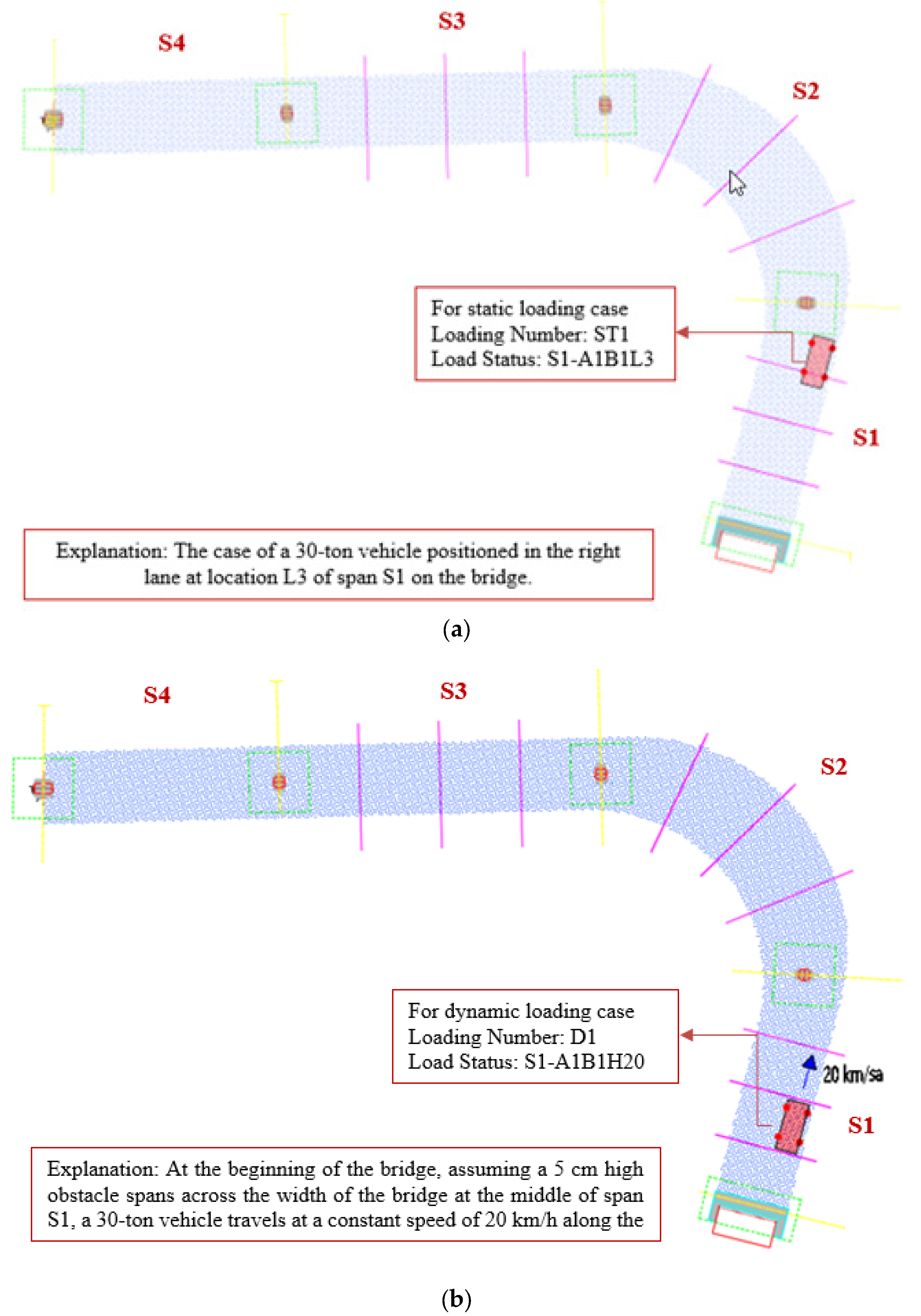
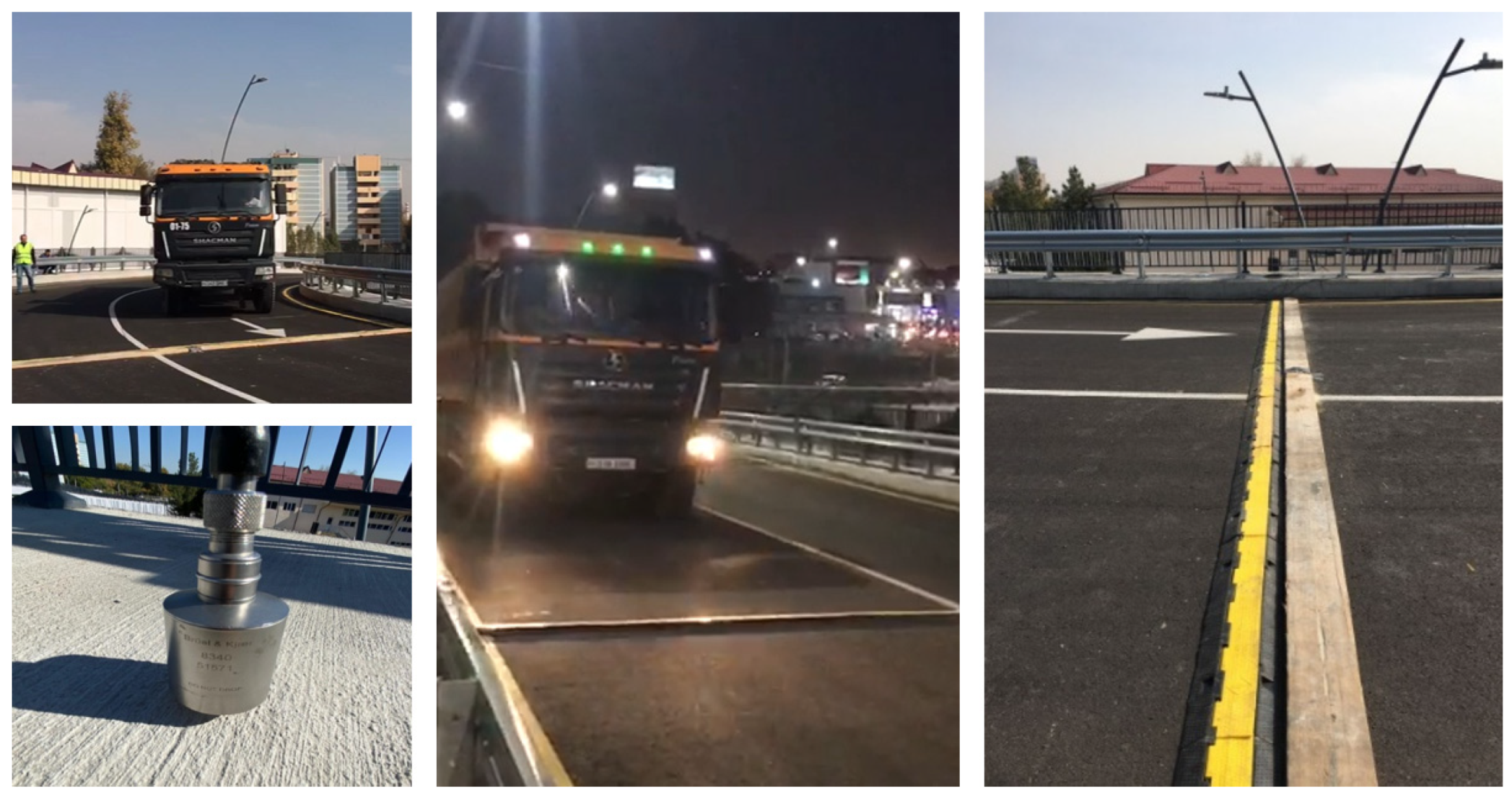
2.3. Static Vehicle Loading Test

Static vehicle load tests are one of the most commonly used methods for evaluating the structural performance of bridges and verifying the accuracy of their design. These tests provide an opportunity to directly observe the behavior of the structure under controlled loads applied to the bridge. One of the most significant advantages of static load tests is their ability to reliably assess whether parameters, such as stresses and displacements experienced by bridge elements, remain within the design-specified limits. Additionally, the data obtained during these tests serve as a fundamental dataset for the update of finite-element models of bridges, enabling more accurate simulations to be performed.

Before starting the static vehicle load tests on the Cho’ponota L1 Bridge, the displacement values of the bridge were obtained based on the local coordinates of the marked points on the underside of the deck (

Table 3. Initial Local Coordinates of Cho’ponota L1 Bridge.

Bridge Span	Measurement No.	X (m)	Y (m)	Z (m)
S1	S1-L11	19,804.621	69,512.946	422.621
	S1-L13	19,805.154	69,509.487	421.790
	S1-L15	19,805.679	69,506.027	422.522
	S1-L21	19,796.466	69,511.709	423.096
	S1-L23	19,796.993	69,508.247	422.281
	S1-L25	19,797.515	69,504.791	423.011
	S1-L31	19,788.310	69,510.475	423.525
	S1-L33	19,788.832	69,507.011	422.711
	S1-L35	19,789.362	69,503.558	423.443
S2	S2-L11	19,768.148	69,503.033	423.978
	S2-L13	19,771.272	69,499.468	423.406
	S2-L15	19,774.519	69,495.767	424.000
	S2-L21	19,760.482	69,491.887	424.003
	S2-L23	19,765.012	69,490.213	423.469
	S2-L25	19,769.731	69,488.464	424.115
	S2-L31	19,758.939	69,479.325	424.100
	S2-L33	19,763.121	69,479.207	423.540
	S2-L35	19,767.639	69,479.081	424.125
S3	S3-L11	19,767.618	69,456.812	423.793
	S3-L13	19,770.541	69,458.130	423.051
	S3-L15	19,773.634	69,459.519	423.825
	S3-L21	19,772.235	69,446.555	423.302
	S3-L23	19,775.165	69,447.874	422.572
	S3-L25	19,778.256	69,449.268	423.408
	S3-L31	19,776.851	69,436.301	422.772
	S3-L33	19,779.783	69,437.615	422.049
	S3-L35	19,782.872	69,439.006	422.886

). The displacement values provided in Table 3 are important as they will serve as a reference source for potential experimental test studies on bridges in the coming years.

Following this preliminary work, a total of 28 different loading scenarios were conducted as part of the static vehicle load tests on the three spans of the bridge using trucks weighing 30 tons and 50 tons. These loading scenarios were carefully planned to identify the displacement values that could occur in various parts of the bridge. Additionally, evaluating the effects of trucks with different weights at different locations allows for the simulation of possible conditions the bridge may encounter throughout its service life. In the test procedure, after positioning the trucks at the designated locations on each span, a waiting period of at least 15 min was observed before starting the test. This waiting time was necessary to ensure that the dynamic stress fluctuations caused by the truck’s movement as it approached the designated region of the bridge completely dissipated. For each loading scenario, geodetic displacement values were recorded at designated points on the bridge using the total station. Some images from the static vehicle load tests conducted on the bridge are presented in Figure 6. The displacement values obtained from the static load tests on the Cho’ponota L1 Bridge are presented in

Table 4. Displacement values obtained from static loading tests on the Cho’ponota L1 Bridge (all displacement values are indicated in millimeters (mm)).

Bridge Span	Loading Status	L11	L13	L15	L21	L23	L25	L31	L33	L35
S1	ST1	−2	−1	−1	−3	−2	−2	−2	−1	0
	ST2	−3	−2	−2	−5	−4	−4	−2	−2	−1
	ST3	−1	−1	−2	−2	−2	−3	−2	−2	−1
	ST4	−2	−2	−3	−3	−4	−5	−2	−2	−2
	ST5	−3	−2	−2	−5	−4	−4	−4	−3	−2
	ST6	−5	−4	−3	−8	−6	−6	−5	−4	−2
	ST7	−2	−2	−3	−4	−4	−5	−3	−3	−3
	ST8	−3	−4	−5	−5	−6	−7	−3	−4	−4
S2	ST9	−7	−5	1	−11	−6	1	−5	−2	1
	ST10	−8	−5	0	−16	−10	−1	−9	−5	−1
	ST11	−4	−3	2	−10	−6	1	−8	−4	0
	ST12	−4	−3	1	−8	−4	2	−4	−1	2
	ST13	−5	−4	0	−11	−6	0	−6	−3	0
	ST14	−3	−2	2	−8	−4	3	−5	−2	1
	ST15	−11	−7	1	−16	−9	0	−8	−3	1
	ST16	−15	−10	−3	−27	−17	−5	−16	−9	−3
	ST17	−9	−6	1	−20	−12	−1	−15	−9	−2
	ST18	−8	−6	−1	−13	−8	0	−7	−3	1
	ST19	−11	−8	−3	−19	−13	−5	−12	−8	−3
	ST20	−9	−5	0	−16	−10	−1	−11	−7	−3
S3	ST21	−5	−5	−4	−5	−4	−4	−3	−2	−1
	ST22	−5	−4	−4	−7	−5	−6	−5	−3	−2
	ST23	−4	−5	−6	−4	−5	−6	−2	−2	−3
	ST24	−3	−5	−6	−5	−6	−9	−4	−4	−6
	ST25	−7	−7	−6	−7	−6	−5	−5	−3	−2
	ST26	−8	−7	−7	−12	−10	−10	−8	−6	−5
	ST27	−6	−8	−10	−7	−8	−10	−4	−4	−5
	ST28	−7	−9	−10	−10	−12	−16	−6	−7	−10

.

When examining the values recorded at different locations and loading scenarios for each span, it was observed that span S2 exhibited higher displacement values compared to the other spans. During the construction phase, periodic measurements also indicated displacement values exceeding the expected limits. Considering this issue, the 100-ton truck, which was used in the design phase, was not utilized in the tests to avoid any potential problems regarding the bridge’s usability. Following the conducted tests, analyses will be performed using the updated finite-element model with the 100-ton vehicle to evaluate the condition of the bridge. This approach ensures that the structural performance of the bridge under the heavier design load can be evaluated without introducing unnecessary risks during the actual testing phase.

2.4. Dynamic Vehicle Loading Test

Dynamic vehicle load tests are an important method used to evaluate the effects of moving loads that bridges will experience throughout their service life. These tests provide significant advantages for understanding the dynamic behavior of the bridge and determining parameters such as acceleration, displacement, and stress in structural elements. The most significant advantage of dynamic load tests is the ability to measure the real-time effects of moving loads on the bridge and to analyze the vibration performance of the structure in detail. Additionally, by applying different speed and load scenarios, the bridge’s response under varying conditions can be examined. This allows the behavior of the bridge within its design limits to be verified and its structural performance to be reliably assessed.

In this study, as part of the dynamic vehicle load tests, two trucks weighing 30 tons (A1) and 50 tons (A2) were used on the three spans of the bridge (Figure 7). The tests were conducted with each vehicle moving at two different speeds (20 km/h and 30 km/h) at various locations on the bridge. Additionally, acceleration data were recorded in detail as the vehicles passed over a 5 cm-high obstacle located at the midspan of the respective spans, in both the right and left lanes. A total of 24 different loading scenarios were considered.

During the tests, B&K8340 accelerometer sensors were installed at designated points on the bridge to record acceleration data, and measurements were conducted using the B&K Type 3560C data acquisition unit. The dynamic responses (acceleration values) of the bridge were recorded in real time as the vehicles moved at different speeds and passed over the obstacle. These data were used to determine the bridge’s dynamic acceleration, velocity, and displacement values.

These tests enabled the evaluation of sudden load changes on the bridge and the vibration behavior of structural elements. Furthermore, measurements taken at different speeds and loads provided a comparative assessment of the performance of bridge components under varying conditions.

During the dynamic load tests, acceleration data for each loading scenario was obtained using accelerometer sensors. After filtering the raw acceleration data, acceleration, velocity, and displacement graphs were generated. Figure 8 presents the acceleration, velocity, and displacement graphs for point S1-L11 under the D1 loading condition. For visualization purposes, the acceleration, velocity, and displacement signals presented in Figure 8 were processed using filtering and peak envelope extraction techniques to highlight maximum response tendencies. This approach allows for an easier comparison of relative magnitudes across different domains but does not reflect the raw time-domain phase relationships. The maximum displacement values obtained for all dynamic loading scenarios are provided in

Table 5. Displacement values obtained from dynamic loading tests on the Cho’ponota L1 Bridge (all displacement values are indicated in millimeters (mm)).

Bridge Span	Loading Status	L11	L21	L31	L15	L25	L35
S1	D1	2.86	3.8	2.09	3.29	3.91	2.16
	D2	2.21	2.89	1.59	2.36	2.82	1.6
	D3	0.45	0.88	0.47	0.69	0.79	0.55
	D4	0.52	0.71	0.4	0.57	0.7	0.43
	D5	1.25	1.6	0.95	1.39	1.63	0.97
	D6	1.33	1.71	1.09	1.23	1.4	0.47
	D7	0.57	0.69	0.39	0.83	0.9	0.55
	D8	0.95	1.43	0.92	1.01	1.31	0.66
S2	D9	1.35	2.39	1.47	0.64	1.09	0.88
	D10	1.34	2.19	1.6	1.35	1.89	1.27
	D11	1.13	1.19	0.91	0.49	0.75	0.46
	D12	1.07	1.57	1	0.93	1.57	1.18
	D13	1.58	2.32	1.75	0.61	0.79	0.74
	D14	1.59	2.38	1.62	1.52	2.34	1.57
	D15	1.62	1.79	1.49	0.78	0.91	0.59
	D16	1.21	2.05	1.56	1.39	1.99	1.41
S3	D17	1.19	1.79	0.99	0.94	1.85	0.99
	D18	1.52	1.87	1.1	1.31	1.76	1.12
	D19	0.88	1.43	1.32	0.93	1.16	0.84
	D20	0.99	1.63	1.2	1.06	1.58	1.2
	D21	1.17	1.81	1.33	1.53	1.76	1.08
	D22	1.49	1.84	1.13	1.17	1.71	1.21
	D23	1.12	1.75	1.31	1.06	1.52	0.88
	D24	1.34	2.49	1.91	1.45	2.52	1.53

.

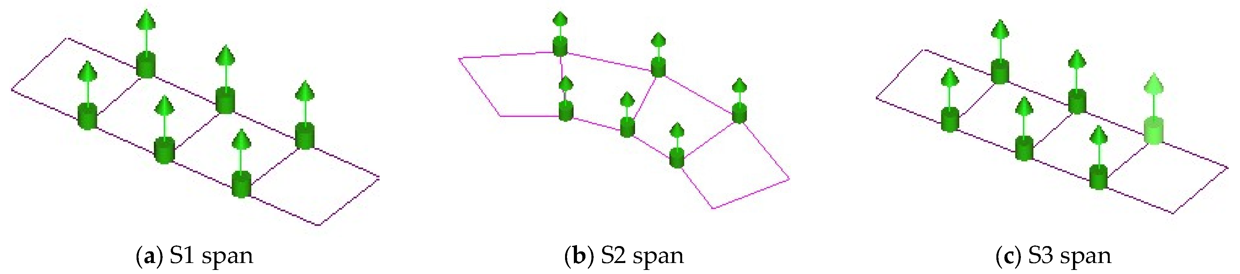
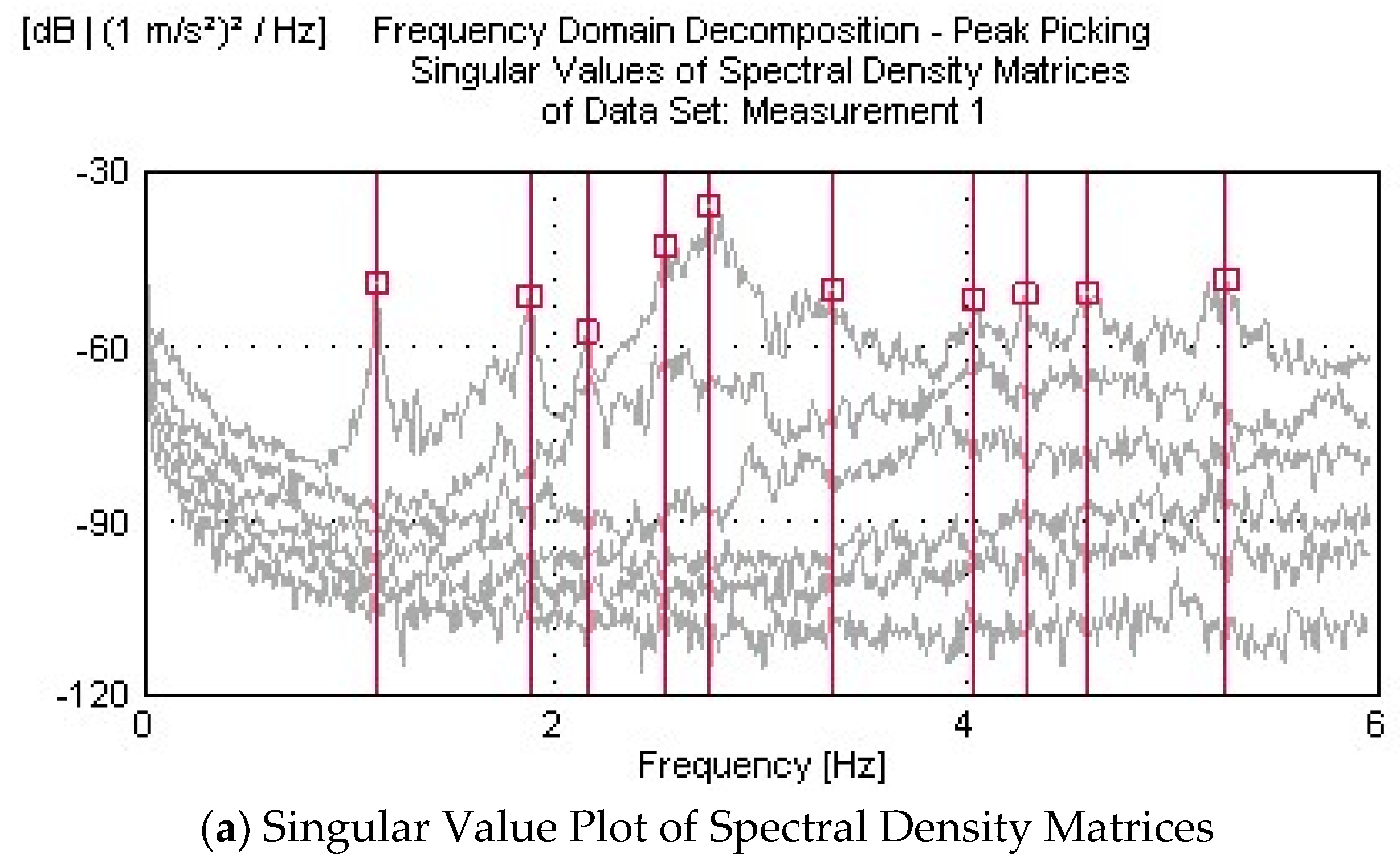
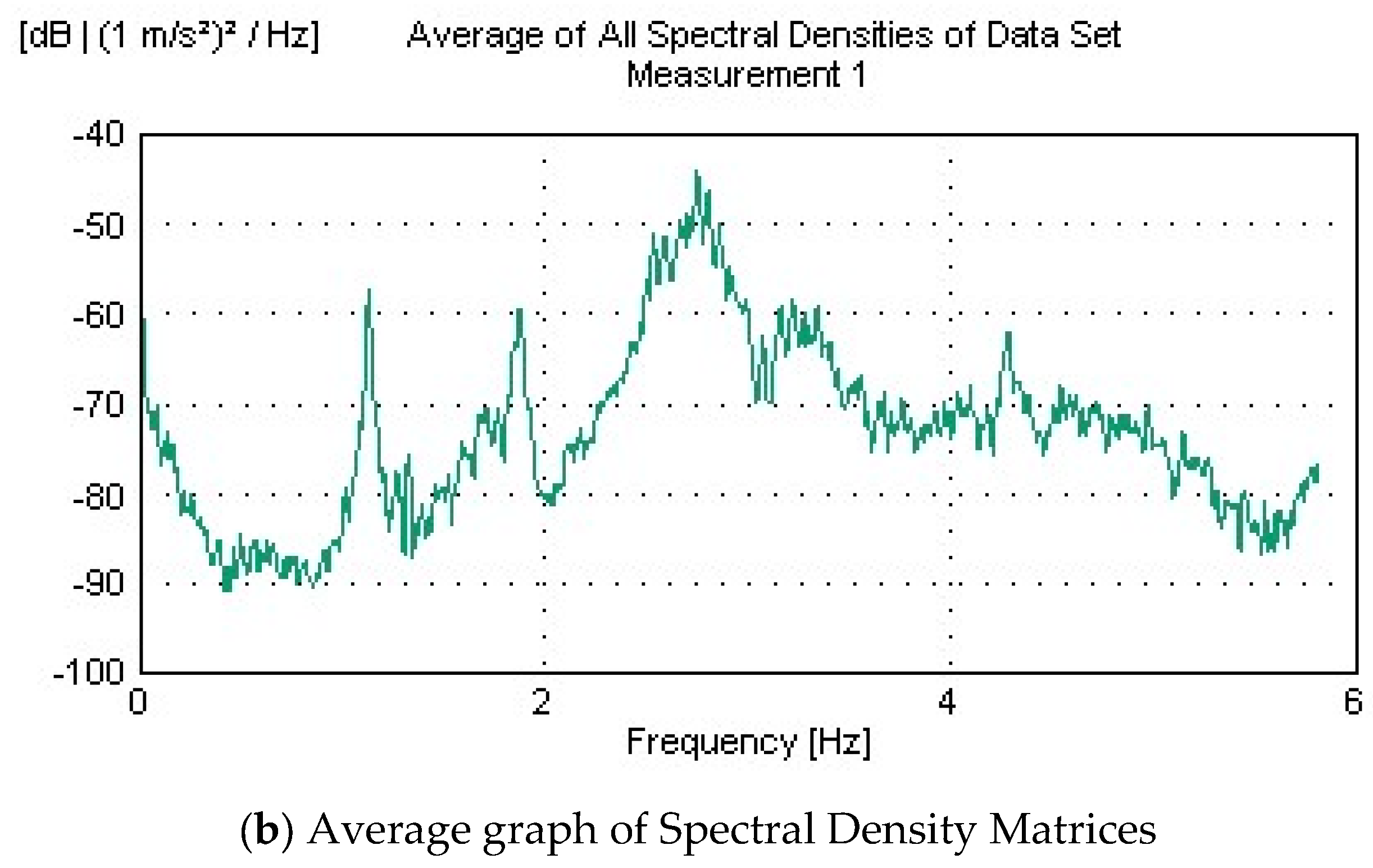
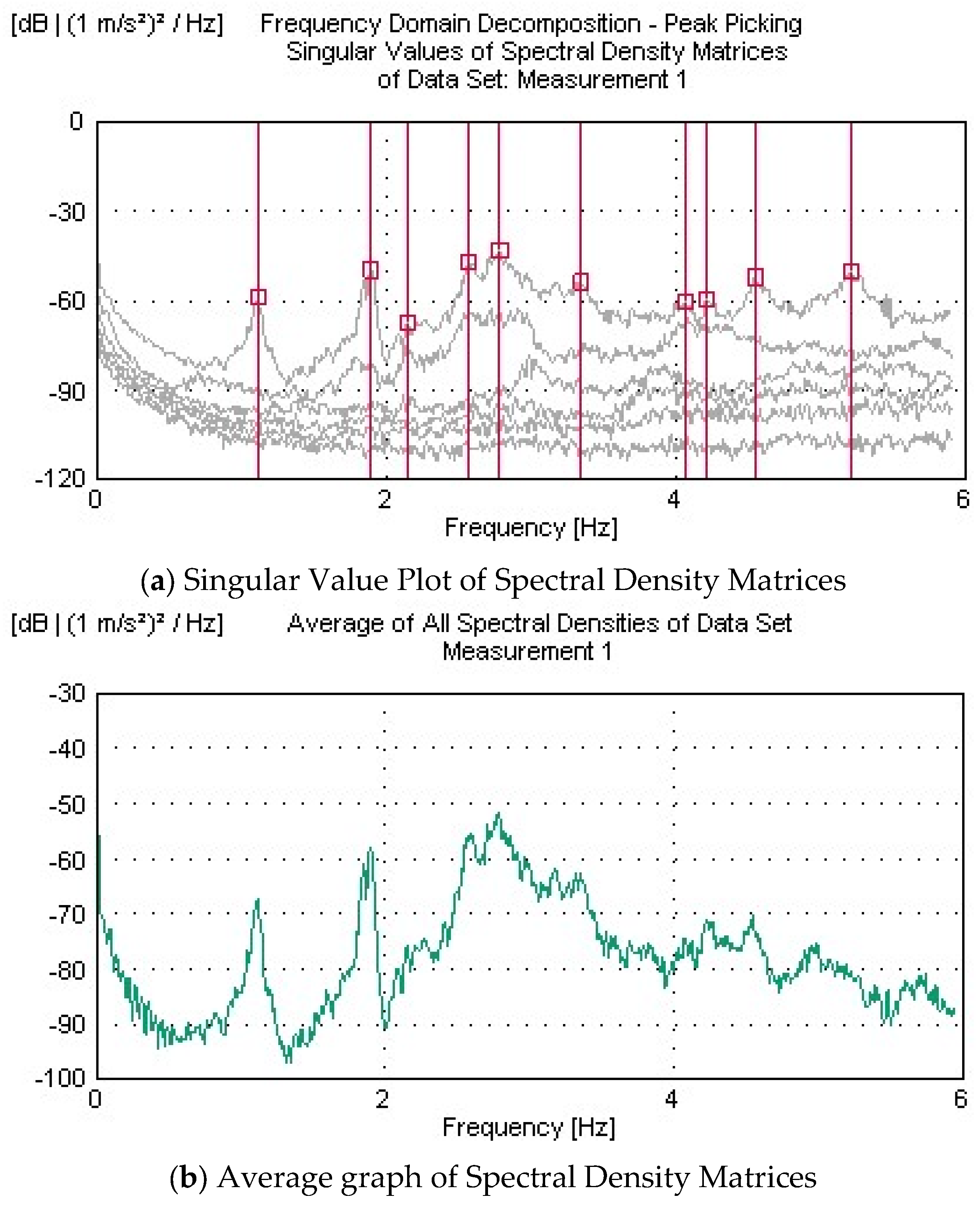
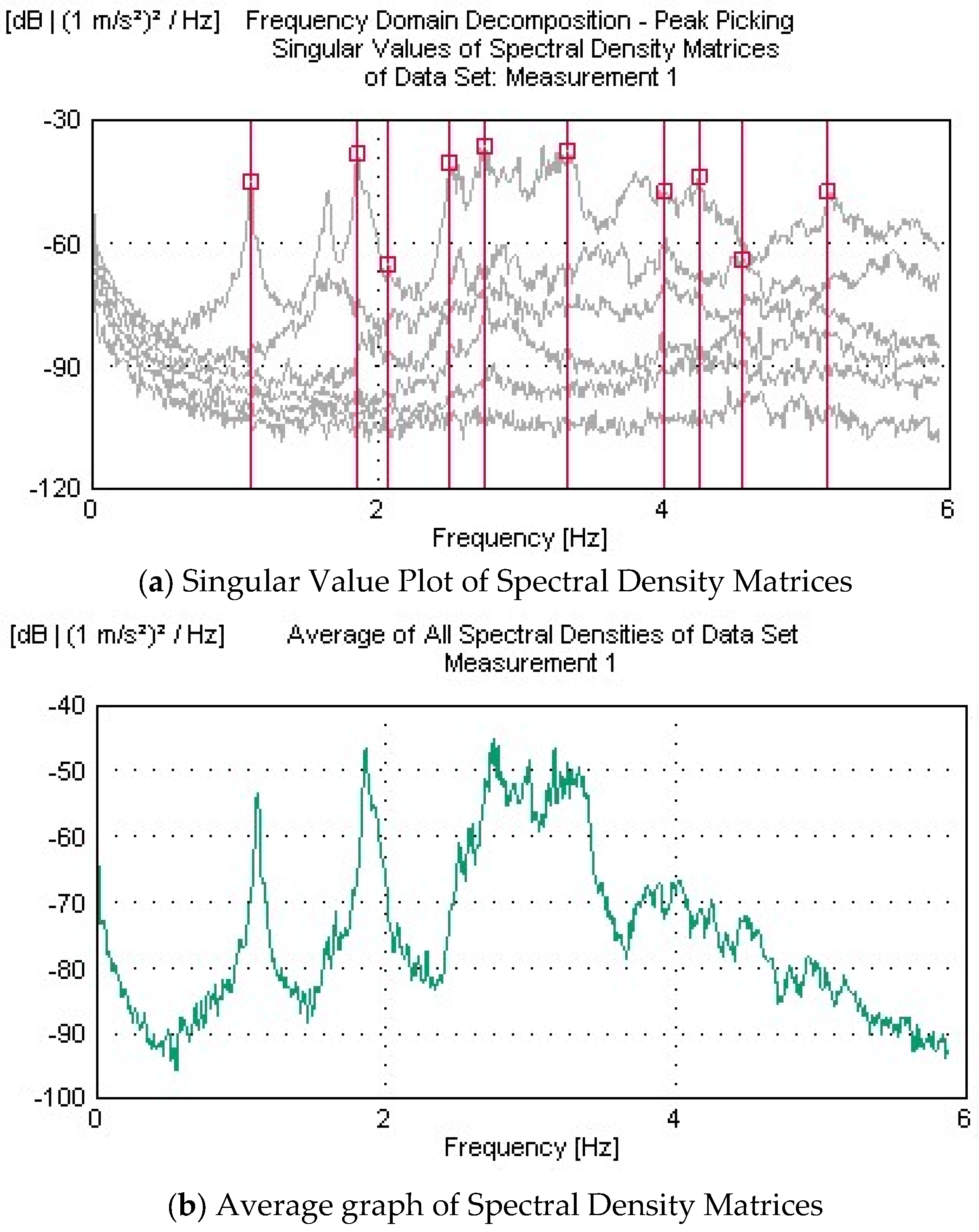
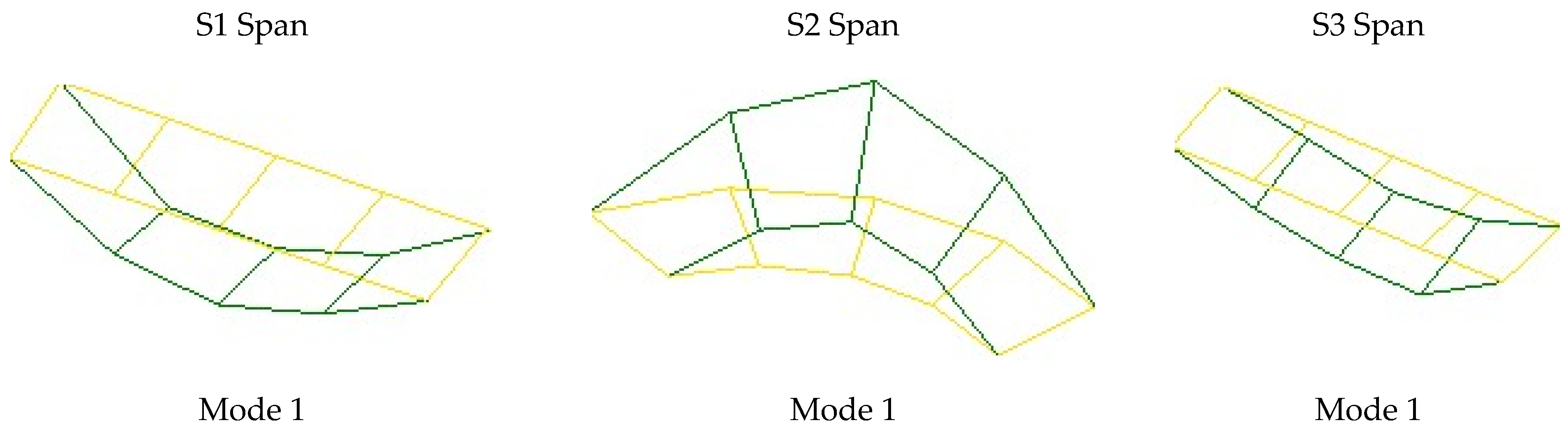
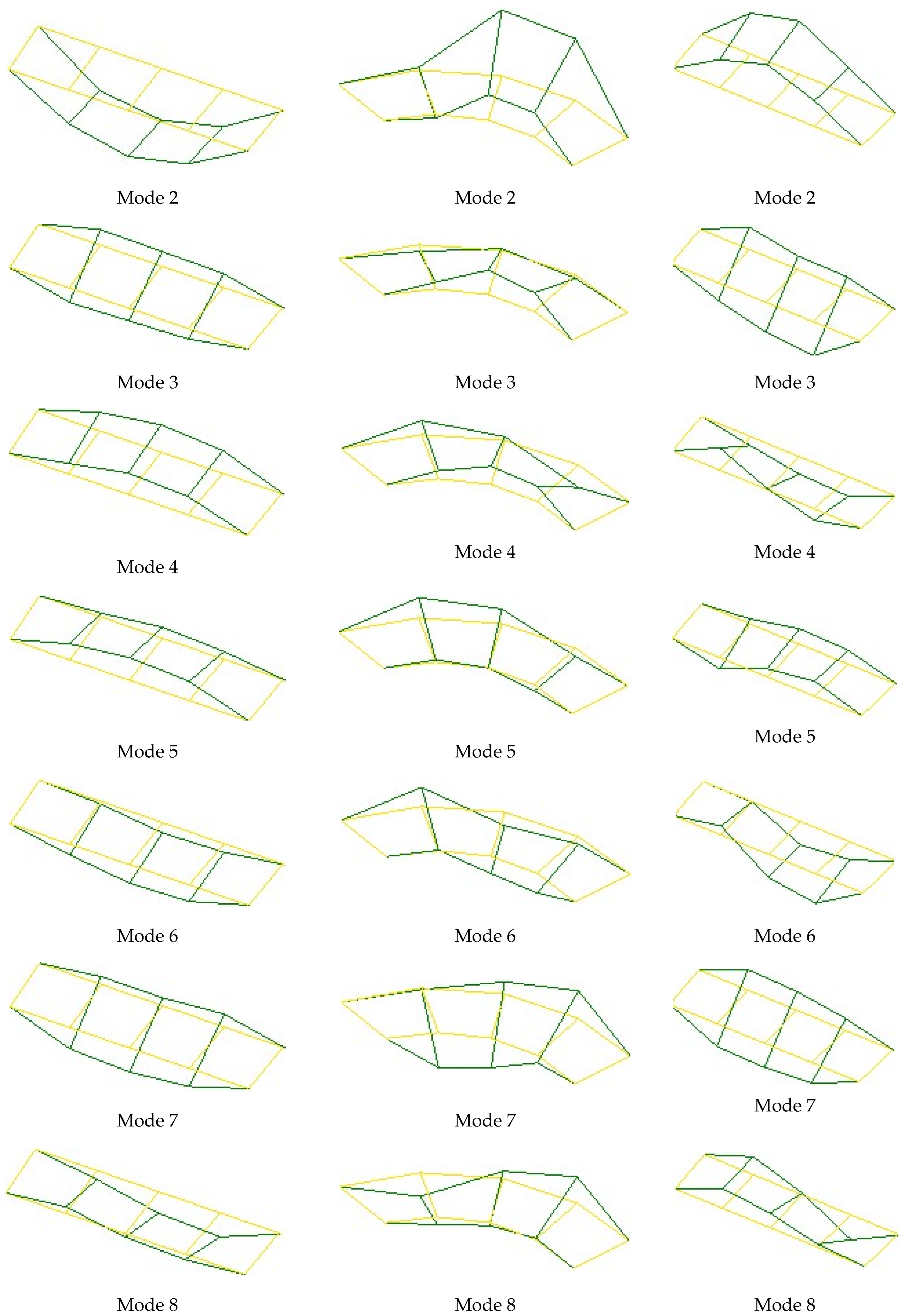
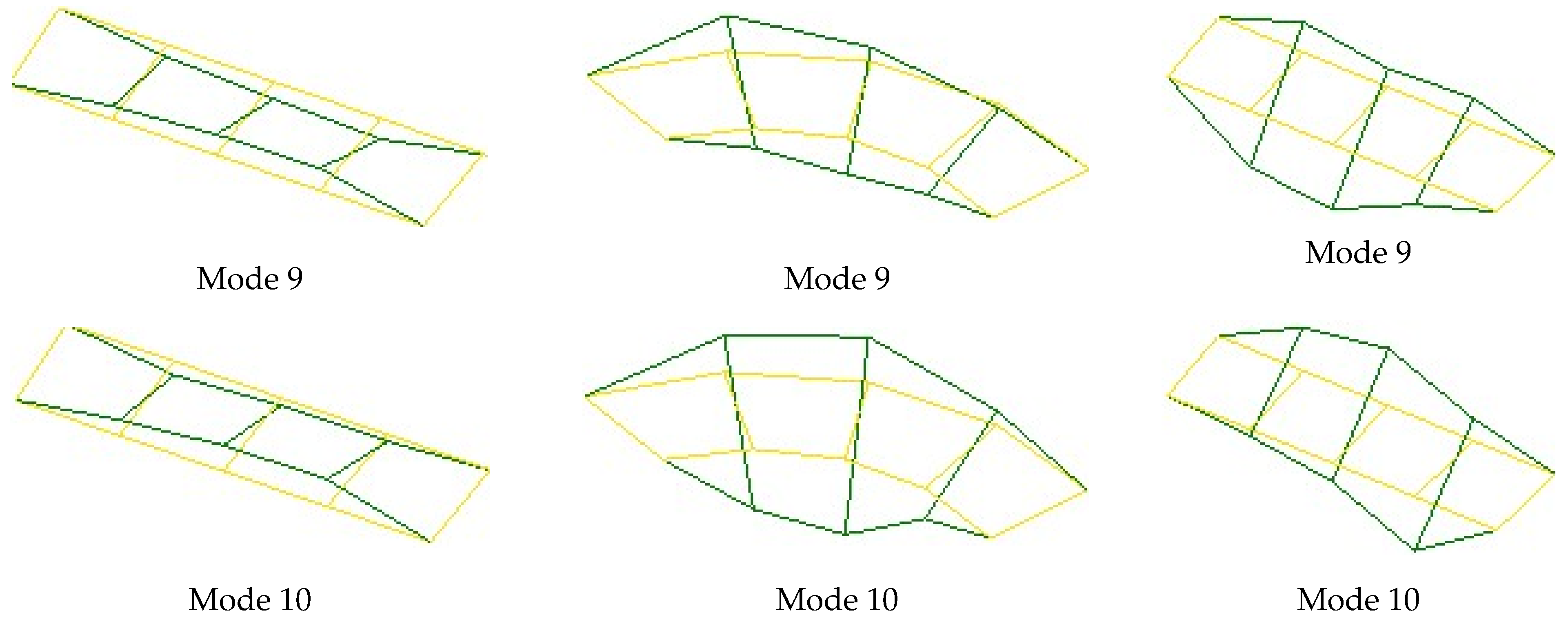
2.5. Operational Modal Analysis Tests

This section presents the details and results of the OMA conducted to determine the structural behavior of the bridge in its current state, specifically focusing on its dynamic characteristics, such as frequencies and mode shapes. Dynamic characteristics are also referred to as the behavior exhibited by the structure under environmental or forced vibrations and are unique to each structure. These characteristics are particularly important as they serve as an indicator of whether a finite-element model (FEM), which is created as a three-dimensional representation in a computer environment, accurately represents the constructed, real structure. Therefore, the results obtained from the finite-element model and the operational measurements must be closely aligned.

For the OMA tests of the Cho’ponota L1 Bridge, sensitive accelerometers were placed at specific points on the bridge. The locations of the accelerometers were determined based on the mode shapes obtained from the modal analysis of the bridge’s initial finite-element model. Figure 9 presents the mode shapes corresponding to the first 10 bending modes obtained from the initial finite-element model of the Cho’ponota L1 Bridge.

In Figure 9, mode shapes with different amplitudes are observed for each mode in the finite-element model of the bridge, and each span moves in distinct patterns. Based on this visualization, the placement of accelerometers in spans S1, S2, and S3 of the bridge has been determined. Figure 10 summarizes the accelerometer placement plan for spans S1, S2, and S3 of the bridge.

In each span, six sensitive accelerometers were placed at equal intervals in the vertical direction to capture the bending modes. The tests used B&K 8340 type single-axis accelerometers, with a dynamic range of 120 dB and a frequency range of 0–1500 Hz. The raw signals captured by these high-sensitive sensors were recorded using the B&K Type 3560C data acquisition unit and transferred to the PULSE Labshop Software Release 11.2 [82]. The raw signals processed in PULSE Labshop were then transferred to Dynamic Modal Release 1.0 [83] and Operational Modal Analysis Software Release 4.0 [84], where they were digitized using frequency and time domain methods to obtain the structure’s frequencies and mode shapes.

In the OMA tests conducted separately for the three spans, the first 10 frequency values and mode shapes of the bridge were determined. The frequency range was selected as 0–8 Hz, and measurements were taken for 15 min per span, resulting in a total measurement duration of 45 min.

The OMA measurements were repeated twice, once before and once after the loading tests. The frequencies and mode shapes obtained prior to the loading tests were accepted as the reference values of the bridge. The results of the measurements conducted after the loading tests were compared with these reference values to determine whether any damage occurred in the structure due to the loading tests. In the conducted OMA tests, the Singular Values of the Spectral Density Matrices (SYMSV) obtained from all measurements for each span are presented in Figure 11, Figure 12, Figure 13, Figure 14, Figure 15 and Figure 16.

As a result of the OMA tests conducted on the Cho’ponota L1 Bridge, the operational mode shapes obtained for each span were found to be consistent with the mode shapes from the finite-element model. The visuals of the first 10 bending mode shapes for the three spans of the bridge are presented in Figure 17.

The frequency values obtained from the OMA tests conducted on the bridge before and after the vehicle loading tests are comprehensively summarized for each span in

Table 6. Frequency values obtained before and after the loading test for S1, S2, and S3 spans.

Mode No.	Frequency Values for S1, S2, and S3 Spans (Hz)
	S1 Span		Diff. (%)	S2 Span		Diff. (%)	S3 Span		Diff. (%)
	Before Loading	After Loading		Before Loading	After		Before	After
1	1.12	1.11	0.89	1.12	1.11	0.89	1.12	1.11	0.89
2	1.87	1.89	1.07	1.89	1.88	0.53	1.89	1.86	1.59
3	2.12	2.12	0.00	2.13	2.13	0.00	2.12	2.07	2.36
4	2.53	2.57	1.58	2.51	2.54	1.20	2.56	2.51	1.95
5	2.75	2.78	1.09	2.75	2.75	0.00	2.74	2.75	0.36
6	3.34	3.35	0.30	3.35	3.34	0.30	3.35	3.34	0.30
7	4.03	4.07	0.99	4.04	4.03	0.25	4.04	4.02	0.50
8	4.28	4.25	0.70	4.28	4.25	0.70	4.25	4.25	0.00
9	4.58	4.55	0.66	4.57	4.53	0.88	4.55	4.55	0.00
10	5.26	5.23	0.57	5.25	5.23	0.38	5.28	5.23	0.95

. As detailed in Table 6, the comparison of frequency values derived from OMA measurements before and after the loading tests reveals a maximum of 1.95%. This maximum value suggests that the structural integrity of the bridge remains largely unaffected by the vehicle loading tests. These findings are critical as they confirm the bridge’s resilience and capability to withstand operational stresses without significant alterations in its dynamic characteristics. Furthermore, the consistency in frequency responses across different spans not only reinforces the reliability of the OMA testing methodology but also supports the bridge’s design assumptions. Such results are instrumental for validating the structural modeling and can guide future maintenance and monitoring strategies to ensure continued safety and performance.

3. Digital Twin Calibration and Validation

The calibration and validation of the digital twin for the Cho’ponota L1 Bridge were conducted by integrating high-fidelity field data into a finite-element model, originally developed using design project documentation. The dynamic characteristics obtained from OMA were compared with the numerical modal properties predicted by the initial finite-element model. Modal analysis results provided natural frequencies and mode shapes for each span, which were also used to guide sensor placement and evaluate the bridge’s dynamic behavior more precisely. As presented in

Table 7. Comparison of operational frequency values for S1, S2, and S3 spans with the initial finite-element model.

Mode No.	Frequency Values for S1, S2, and S3 Spans (Hz)
	Initial FEM	S1		S2		S3		Max. Diff. (%)
		Before Loading	After Loading	Before Loading	After Loading	Before Loading	After Loading
1	0.99	1.12	1.11	1.12	1.11	1.12	1.11	11.61
2	1.64	1.87	1.89	1.89	1.88	1.89	1.86	13.22
3	1.90	2.12	2.12	2.13	2.13	2.12	2.07	10.80
4	2.35	2.53	2.57	2.51	2.54	2.56	2.51	8.56
5	2.82	2.75	2.78	2.75	2.75	2.74	2.75	2.48
6	3.15	3.34	3.35	3.35	3.34	3.35	3.34	5.97
7	3.78	4.03	4.07	4.04	4.03	4.04	4.02	7.13
8	4.34	4.28	4.25	4.28	4.25	4.25	4.25	1.40
9	4.42	4.58	4.55	4.57	4.53	4.55	4.55	3.49
10	5.13	5.26	5.23	5.25	5.23	5.28	5.23	2.84

, the initial model exhibited a maximum frequency discrepancy of 13.22% compared to the OMA results, exceeding the 5% threshold commonly accepted in the literature [85]. These deviations indicated a clear need for model refinement. Such differences often stem from simplifications in modeling assumptions, variations in construction materials, support boundary conditions, or unmodeled as-built deviations. Accordingly, the FE model was iteratively updated—particularly by adjusting material stiffness and support representations—to achieve better alignment with the measured data. One critical hypothesis considered was the potential difference in the actual concrete quality used during construction compared to the project specifications. Through this calibration process, the digital twin was validated as a reliable representation of the bridge’s true dynamic behavior, enabling diagnostic and predictive analyses under service conditions.

The primary updating parameter was selected as the concrete material strength. Manual calibration was performed by incrementally adjusting this property until the natural frequencies derived from the numerical model closely matched those obtained from field measurements. This adjustment reflects the hypothesis that the concrete used during construction may differ from the design values. Through iterative updates, the FE model was refined to accurately represent the actual stiffness distribution of the bridge.

Table 8. Comparison of frequency values for S1, S2, and S3 spans with the updated finite-element model.

Mode No.	Frequency Values for S1, S2, and S3 Spans (Hz)
	Updated FEM	S1		S2		S3		Max. Diff. (%)
		Before Loading	After Loading	Before Loading	After Loading	Before Loading	After Loading
1	1.08	1.12	1.11	1.12	1.11	1.12	1.11	4.17
2	1.80	1.87	1.89	1.89	1.88	1.89	1.86	5.00
3	2.03	2.12	2.12	2.13	2.13	2.12	2.07	4.93
4	2.57	2.53	2.57	2.51	2.54	2.56	2.51	2.33
5	2.88	2.75	2.78	2.75	2.75	2.74	2.75	4.86
6	3.41	3.34	3.35	3.35	3.34	3.35	3.34	2.05
7	4.07	4.03	4.07	4.04	4.03	4.04	4.02	1.23
8	4.70	4.28	4.25	4.28	4.25	4.25	4.25	9.57
9	4.79	4.58	4.55	4.57	4.53	4.55	4.55	5.01
10	5.50	5.26	5.23	5.25	5.23	5.28	5.23	4.91

presents the comparison of the updated model’s frequency values with OMA data. The results indicate that, for all modes except the eighth, frequency deviations were reduced below 5%, thus meeting widely accepted validation criteria. Even the eighth mode—where deviation slightly exceeds 5%—remains within tolerable limits for higher-order modes. This calibration process confirms the digital twin’s fidelity and supports its utility for structural assessment, simulation, and future diagnostic applications.

4. Evaluation of Test Results

The comparison and evaluation of all experimental and numerical results from the vehicle load tests and OMA measurements of the Cho’ponota L1 Bridge are summarized in four parts: (1) evaluation of static displacement data, (2) evaluation of dynamic displacement data, (3) linearity check, and (4) assessment of the current condition.

4.1. Static Deformation Data

In the static load tests, a total of 28 static loading cases were considered, including 8 cases for span S1, 12 cases for span S2, and 8 cases for span S3. For each loading case, displacement results obtained from the 9 designated points along the cross-section and length of the deck were compared between the static vehicle load tests and the updated finite-element model analysis, as shown in

Table 9. Comparison of displacement results obtained from static vehicle loading test (Test) and finite element model (FEM).

Bridge Span	Loading Status	Displacement Results Obtained from Test and FEM (mm)
		L11		L13		L15		L21		L23		L25		L31		L33		L35
		Test	FEM	Test	FEM	Test	FEM	Test	FEM	Test	FEM	Test	FEM	Test	FEM	Test	FEM	Test	FEM
S1	ST1	−2	−2.28	−1	−1.87	−1	−1.46	−3	−3.77	−2	−3.00	−2	−2.22	−2	−3.53	−1	−2.53	0	−1.43
	ST2	−3	−3.79	−2	−3.20	−2	−2.62	−5	−5.56	−4	−4.66	−4	−3.62	−2	−3.62	−2	−2.96	−1	−2.28
	ST3	−1	−1.62	−1	−2.08	−2	−2.56	−2	−2.36	−2	−3.25	−3	−4.12	−2	−1.13	−2	−2.38	−1	−2.48
	ST4	−2	−2.64	−2	−3.40	−3	−4.16	−3	−3.54	−4	−4.89	−5	−6.12	−2	−1.78	−2	−2.92	−2	−3.03
	ST5	−3	−3.80	−2	−3.11	−2	−2.43	−5	−6.29	−4	−4.95	−4	−3.71	−4	−5.89	−3	−4.22	−2	−2.39
	ST6	−5	−6.32	−4	−5.35	−3	−4.36	−8	−9.27	−6	−7.76	−6	−6.04	−5	−6.05	−4	−4.93	−2	−3.80
	ST7	−2	−2.69	−2	−3.48	−3	−4.27	−4	−3.94	−4	−5.42	−5	−6.88	−3	−1.87	−3	−3.97	−3	−5.89
	ST8	−3	−4.40	−4	−5.67	−5	−6.93	−5	−5.90	−6	−8.16	−7	−10.20	−3	−2.96	−4	−4.85	−4	−5.42
S2	ST9	−7	−8.30	−5	−5.72	1	−3.05	−11	−10.31	−6	−6.92	1	−3.62	−5	−4.93	−2	−3.44	1	−1.94
	ST10	−8	−8.77	−5	−6.48	0	−4.26	−16	−16.54	−10	−10.25	−1	−6.09	−9	−10.34	−5	−7.32	−1	−4.29
	ST11	−4	−4.38	−3	−3.16	2	−1.91	−10	−10.32	−6	−6.82	1	−3.30	−8	−9.92	−4	−6.85	0	−2.97
	ST12	−4	−3.20	−3	−3.68	1	−3.94	−8	−4.45	−4	−4.34	2	−4.67	−4	−2.55	−1	−2.15	2	−2.35
	ST13	−5	−4.53	−4	−4.46	0	−4.35	−11	−8.51	−6	−7.06	0	−6.75	−6	−6.27	−3	−4.74	0	−4.33
	ST14	−3	−2.04	−2	−2.19	2	−2.34	−8	−4.62	−4	−4.40	3	−4.21	−5	−3.95	−2	−3.64	1	−3.92
	ST15	−11	−13.85	−7	−9.53	1	−5.08	−16	−17.18	−9	−10.85	0	−6.04	−8	−8.20	−3	−5.74	1	−3.23
	ST16	−15	−14.61	−10	−10.88	−3	−7.10	−27	−27.57	−17	−18.91	−5	−10.15	−16	−17.23	−9	−12.19	−3	−7.14
	ST17	−9	−9.18	−6	−5.26	1	−3.19	−20	−17.21	−12	−11.36	−1	−5.51	−15	−17.79	−9	−11.42	−2	−4.95
	ST18	−8	−6.40	−6	−6.14	−1	−6.56	−13	−9.41	−8	−7.67	0	−7.79	−7	−4.25	−3	−3.58	1	−3.91
	ST19	−11	−9.59	−8	−7.42	−3	−7.24	−19	−18.17	−13	−12.96	−5	−11.25	−12	−8.53	−8	−7.90	−3	−7.22
	ST20	−9	−4.45	−5	−3.65	0	−3.90	−16	−7.72	−10	−7.34	−1	−7.03	−11	−5.24	−7	−6.07	−3	−6.52
S3	ST21	−5	−6.36	−5	−3.98	−4	−1.72	−5	−6.49	−4	−4.40	−4	−2.32	−3	−3.88	−2	−2.24	−1	−0.61
	ST22	−5	−6.09	−4	−4.55	−4	−3.05	−7	−9.39	−5	−7.09	−6	−4.63	−5	−6.19	−3	−4.19	−2	−2.17
	ST23	−4	−0.98	−5	−4.52	−6	−8.22	−4	−2.16	−5	−5.45	−6	−8.75	−2	−0.25	−2	−2.82	−3	−5.40
	ST24	−3	−1.55	−5	−4.98	−6	−8.40	−5	−3.51	−6	−7.90	−9	−12.14	−4	−1.08	−4	−4.62	−6	−7.16
	ST25	−7	−10.60	−7	−6.63	−6	−2.87	−7	−10.81	−6	−7.33	−5	−3.88	−5	−6.47	−3	−3.73	−2	−1.02
	ST26	−8	−10.17	−7	−7.59	−7	−5.01	−12	−15.65	−10	−11.81	−10	−7.71	−8	−10.32	−6	−6.98	−5	−3.62
	ST27	−6	−1.62	−8	−7.54	−10	−13.71	−7	−3.61	−8	−9.09	−10	−14.59	−4	−0.82	−4	−4.71	−5	−9.00
	ST28	−7	−2.59	−9	−8.30	−10	−14.00	−10	−5.85	−12	−13.17	−16	−20.23	−6	−1.79	−7	−7.71	−10	−13.61

.

The uncertainty of the total station measurement device used in the static displacement tests was considered to be in the range of 1.0–1.5 mm, and the evaluations were conducted accordingly. Upon examining Table 9, it can be observed that the displacement values of the deck in the bridge spans are consistent with and very close to the results obtained from the finite-element analysis. However, when analyzing the column corresponding to point L23, located at the center of the spans, it was noted that the displacement values obtained from the static vehicle load tests are slightly smaller than those calculated from the finite-element analysis. This indicates that the actual stiffness of the deck is higher and could be considered safer compared to the finite-element model. This situation is similar to the comparison between the frequency values obtained from the OMA measurements and those derived from the finite-element model.

Based on the results obtained, it is evident that under the 30 t and 50 t vehicle loads, the displacement values from the finite-element analysis and the static vehicle load tests (with a maximum displacement of 17 mm at the midspan for the 50 t vehicle) are close to each other and remain within acceptable limits.

4.2. Dynamic Deformation Data

In the static load tests, a total of 24 dynamic loading cases were performed, with 8 cases for each of spans S1, S2, and S3. During the dynamic loading, a 5 cm-high obstacle was placed at the center of the respective bridge spans to enable vehicle passage. Acceleration data were recorded using accelerometer sensors during vehicle crossings. These data were processed to determine the acceleration, velocity, and displacement values at the relevant points caused by the dynamic loading. Based on the ratio of the dynamic displacement at the specific point to the maximum displacement observed in the static condition, the Dynamic Amplification Factor (DAF) was calculated. The values obtained for the calculation of the Dynamic Amplification Factor from static and dynamic displacement results are presented in

Table 10. Dynamic Amplification Factors (DAF) obtained from static and dynamic deformation results.

Bridge Span	Loading Status	L11			L21			L31			L15			L25			L35
		St.	Dyna.	DAF (%)	St.	Dyna.	DAF (%)	St.	Dyna.	DAF (%)	St.	Dyna.	DAF (%)	St.	Dyna.	DAF (%)	St.	Dyna.	DAF (%)
S1	D1	3	2.86	95.33	5	3.8	76	2	2.09	104.5	2	3.29	164.5	4	3.91	97.75	1	2.16	216
	D2	3	2.21	73.67	5	2.89	57.8	2	1.59	79.5	2	2.36	118	4	2.82	70.5	1	1.6	160
	D3	2	0.45	22.5	3	0.88	29.33	2	0.47	23.5	3	0.69	23	5	0.79	15.8	2	0.55	27.5
	D4	2	0.52	26	3	0.71	23.67	2	0.4	20	3	0.57	19	5	0.7	14	2	0.43	21.5
	D5	5	1.25	25	8	1.6	20	5	0.95	19	4	1.39	34.75	6	1.63	27.17	2	0.97	48.5
	D6	5	1.33	26.6	8	1.71	21.38	5	1.09	21.8	4	1.23	30.75	6	1.4	23.33	2	0.47	23.5
	D7	3	0.57	19	5	0.69	13.8	3	0.39	13	5	0.83	16.6	7	0.9	12.86	4	0.55	13.75
	D8	3	0.95	31.67	5	1.43	28.6	3	0.92	30.67	5	1.01	20.2	7	1.31	18.71	4	0.66	16.5
S2	D9	8	1.35	16.88	16	2.39	14.94	9	1.47	16.33	0	0.64	-	1	1.09	109	1	0.88	88
	D10	8	1.34	16.75	16	2.19	13.69	9	1.6	17.78	0	1.35	-	1	1.89	189	1	1.27	127
	D11	5	1.13	22.6	11	1.19	10.82	6	0.91	15.17	0	0.49	-	0	0.75	-	1	0.46	46
	D12	5	1.07	21.4	11	1.57	14.27	6	1	16.67	0	0.93	-	0	1.57	-	1	1.18	118
	D13	15	1.58	10.53	27	2.32	8.59	16	1.75	10.94	3	0.61	20.33	5	0.79	15.8	0	0.74	-
	D14	15	1.59	10.6	27	2.38	8.81	16	1.62	10.13	3	1.52	50.67	5	2.34	46.8	0	1.57	-
	D15	11	1.62	14.73	19	1.79	9.42	12	1.49	12.42	3	0.78	26	5	0.91	18.2	3	0.59	19.67
	D16	11	1.21	11	19	2.05	10.79	12	1.56	13	3	1.39	46.33	5	1.99	39.8	3	1.41	47
S3	D17	5	1.19	23.8	7	1.79	25.57	5	0.99	19.8	4	0.94	23.5	5	1.85	37	2	0.99	49.5
	D18	5	1.52	30.4	7	1.87	26.71	5	1.1	22	4	1.31	32.75	5	1.76	35.2	2	1.12	56
	D19	3	0.88	29.33	5	1.43	28.6	4	1.32	33	6	0.93	15.5	9	1.16	12.89	6	0.84	14
	D20	3	0.99	33	5	1.63	32.6	4	1.2	30	6	1.06	17.67	9	1.58	17.56	6	1.2	20
	D21	8	1.17	14.63	12	1.81	15.08	8	1.33	16.63	7	1.53	21.86	10	1.76	17.6	5	1.08	21.6
	D22	8	1.49	18.63	12	1.84	15.33	8	1.13	14.13	7	1.17	16.71	10	1.71	17.1	5	1.21	24.2
	D23	7	1.12	16	10	1.75	17.5	6	1.31	21.83	10	1.06	10.6	16	1.52	9.5	10	0.88	8.8
	D24	7	1.34	19.14	10	2.49	24.9	6	1.91	31.83	10	1.45	14.5	16	2.52	15.75	10	1.53	15.3

Values in bold and italics indicate displacements ≤ 3 mm, which were excluded from the Dynamic Amplification Factor calculation to minimize measurement uncertainties.

.

In evaluating the Dynamic Amplification Factor, to minimize errors caused by measurement uncertainties, displacement values 3 mm or less obtained under static loading (marked in bold and italic in Table 10) were excluded from consideration. Out of the 144 measurement points, 52 points with displacements less than 3 mm were excluded, and evaluations were performed based on the remaining 92 points.

According to the AASHTO LRFD 2017 specifications, the permissible DAF value is limited to 33%. As seen in Table 10, four measurement points exceeded this allowable limit. A general evaluation of Table 10 reveals that 100 (92 − 4)/92 = 95.6% of the measurement points remained within the allowable limits, and this ratio was deemed acceptable for the operational use of the bridge.

4.3. Linearity Control

The purpose of the linearity check is to determine whether the bridge exhibits linear behavior under various vehicle loads. In this evaluation, the displacements recorded at the midpoints of the spans due to the effects of 30 t and 50 t vehicles during static vehicle load tests were compared relative to the load ratio.

The values for determining the displacement ratio experimentally, based on vehicle load, are presented in

Table 11. Experimental determination of linearity ratio depending on vehicle load.

Bridge Span	Loading Status	Vehicle Load (KN)	Load Ratio	L23	Displacement Ratio
S1	ST2	300	1.67	−4	1.50
	ST6	500		−6
	ST4	300	1.67	−4	1.50
	ST8	500		−6
S2	ST10	300	1.67	−10	1.70
	ST16	500		−17
	ST13	300	1.67	−6	2.17
	ST19	500		−13
S3	ST22	300	1.67	−5	2.00
	ST26	500		−10
	ST24	300	1.67	−6	2.00
	ST28	500		−12

. Upon examining Table 11, it was observed that as the vehicle load ratio increased (500/300 = 1.67 times), the displacement values changed in the range of 1.5 (6/4) to 2.17 (13/6). This range was considered to be within acceptable levels due to the measurement uncertainty mentioned above.

After all static and dynamic vehicle load tests, the displacement condition of the bridge was checked, and similar values were obtained. This indicates that the bridge behaved linearly during the static and dynamic vehicle load tests, and that there was no significant change in the bridge stiffness that could affect its structural behavior following the tests. Additionally, visual inspections were performed on the bridge after all static and dynamic vehicle load tests, and no deformation or cracks were detected on the structure.

4.4. Current Situation Assessment

After the completion of the Cho’ponota L1 Bridge construction phase, a deflection problem occurred in span S2, and it was requested to verify the compliance of the project and construction through vehicle load tests and non-destructive OMA measurements. For this purpose, the provided finite-element model of the bridge was updated based on the OMA results. The assessment of the current condition has been conducted using this updated model and is presented below.

After the static vehicle load tests, numerical analyses showed that the operational displacement values obtained from the 30 t and 50 t vehicle load tests were consistent with the displacement values obtained from the finite-element analysis for the same loading conditions. This indicates that the finite-element model of the bridge can be reliably considered. In the project calculation report, a displacement value of 41.8 mm was obtained for a 100 t loading condition, and a similar value was derived using the updated finite-element model. Since this value is lower than the limit value of 56.25 mm (45,000/800), it can be stated that the bridge remains safely within usable limits.

5. Digital Twin Implementation Scope and Limitations

The digital twin presented in this study represents a focused, test-assisted implementation developed specifically for the Cho’ponota L1 Bridge. Unlike traditional digital twins that rely on continuous, real-time data streams and persistent cloud-based infrastructure, this approach leverages a high-quality but temporally limited dataset obtained through ambient vibration monitoring and vehicular load testing. By integrating this data into a calibrated finite-element model, we create a virtual representation of the physical bridge that reflects its actual mechanical behavior under service conditions. This enables not only the diagnosis of existing stiffness loss and deformation but also the simulation of performance under hypothetical future scenarios.

This test-driven digital twin framework fills a critical and underexplored niche in the broader landscape of digital twin applications for civil infrastructure. Most existing studies in the field emphasize long-term monitoring and the use of Internet of Things technologies, which are often impractical to implement on a wide scale due to cost, technical complexity, or accessibility constraints. By contrast, the methodology adopted in this study offers a more accessible and scalable alternative, particularly for bridge managers and infrastructure owners who require periodic assessments rather than real-time surveillance. The presented approach demonstrates that even in the absence of continuous sensor data, a reliable and diagnostically valuable digital twin can be established using structured, short-term field testing.

However, this approach also entails certain limitations. First and foremost, the digital twin developed here is inherently static in nature, capturing the bridge’s condition at the time of testing rather than providing ongoing updates. As a result, it cannot autonomously detect temporal changes such as environmental degradation, cumulative fatigue, or progressive damage. Second, the validity of the model is bounded by the range of structural behaviors represented in the collected data; behaviors not triggered during the test campaign—such as extreme seismic responses or long-term thermal effects—are outside the model’s predictive scope. Third, this implementation does not currently incorporate machine learning or data-driven adaptability, which limits its ability to evolve as new data become available.

Despite these limitations, the proposed framework offers a replicable model for asset verification in scenarios where real-time monitoring is either unnecessary or unfeasible. It illustrates how the core principles of digital twins (virtual mirroring, data integration, and predictive simulation) can still be realized using test-based calibration methods. Furthermore, it contributes to bridging the conceptual and operational gap between finite-element model updating and full-fledged digital twin systems. As such, it offers a hybrid path forward for digital twin deployment in civil engineering: one that is both pragmatic and scientifically rigorous.

6. Conclusions

In this study, the structural behavior and performance of the Cho’ponota L1 Bridge were evaluated through static and dynamic vehicle load tests and non-destructive OMA measurements. The primary goal was to investigate the observed deflection issue in span S2 after the completion of construction and assess the compliance of the bridge design and construction with project specifications. The study also introduced a test-assisted digital twin framework as an effective methodology for evaluating existing bridge infrastructure without the need for continuous monitoring systems.

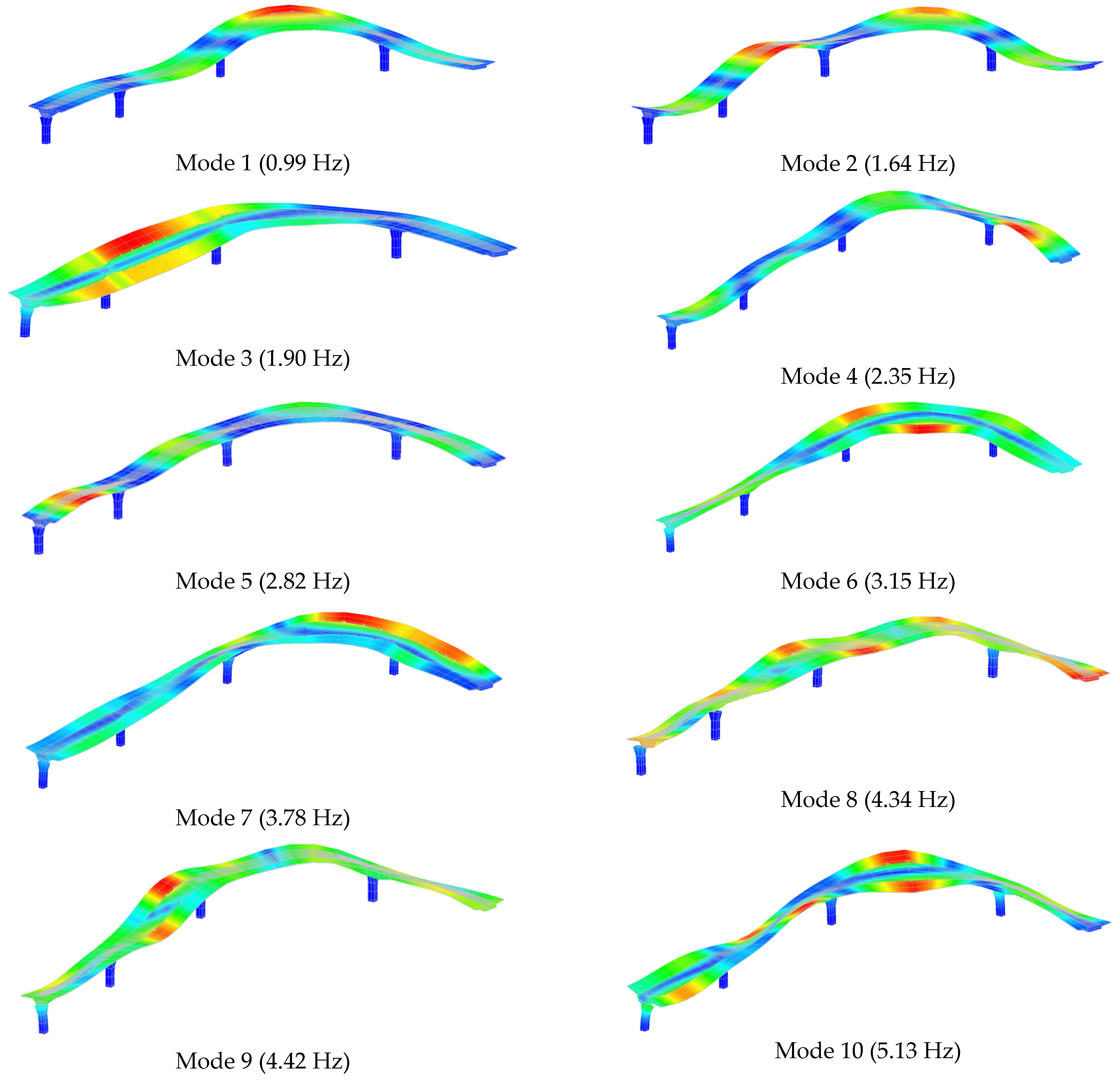
• The initial finite-element model of the bridge was calibrated using the dynamic characteristics (frequencies and mode shapes) obtained from OMA. Differences between the experimental and numerical results, initially as high as 13.22%, were reduced to below 5% through iterative updates to the concrete material properties. This model refinement validated the accuracy of the numerical representation and established a reliable digital twin capable of simulating the actual behavior of the structure.
• Static load tests were performed using 30-ton and 50-ton vehicles under 28 different loading conditions on spans S1, S2, and S3. The displacement values recorded via -the total station were compared to the results of the updated finite-element model. The high degree of agreement between measured and simulated values confirmed the model’s validity. Furthermore, the updated digital twin predicted a displacement of 41.8 mm under the design 100-ton load case, well within the 56.25 mm limit, demonstrating that the bridge operates safely under service loads.
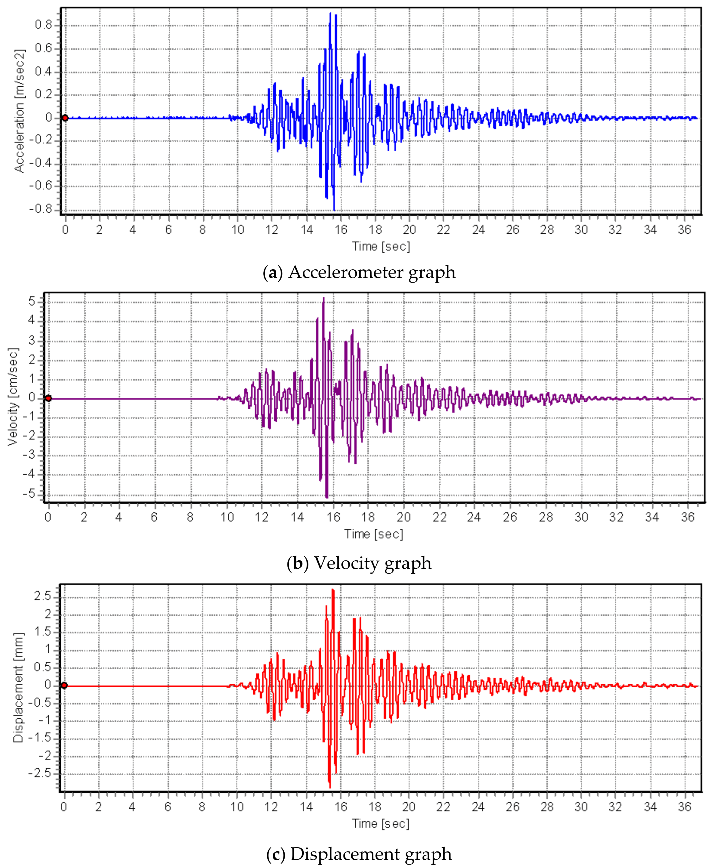
• Dynamic vehicle load tests were conducted across 24 different scenarios using obstacle-induced excitation and two vehicle speeds (20 km/h and 30 km/h). The Dynamic Amplification Factor calculated from accelerometer data complied with the AASHTO LRFD 2017 allowable limit of 33% at 95.6% of the measurement points, indicating that the bridge exhibits stable dynamic behavior under operational loads.
• The linearity of structural response was verified through proportional displacement increases between 30-ton and 50-ton load cases, indicating that the bridge behaves linearly under normal service conditions. Post-test visual inspections revealed no signs of cracking or damage, confirming the structural integrity of the bridge during and after loading.
• In addition to the structural findings, the digital twin constructed in this study offers a validated and test-driven numerical model that can be reused for future decision-making processes. Although it does not operate in real time, the digital twin integrates high-quality field data into a calibrated simulation environment that reflects the actual performance of the bridge. It enables engineers to conduct scenario analyses, predict the impact of different load cases, and plan rehabilitation or strengthening strategies more effectively.
• The test-assisted digital twin approach implemented here bridges the gap between conventional finite-element model updating and real-time monitoring-based digital twin systems. It offers a scalable and economical solution for infrastructure assessment, particularly in contexts where continuous monitoring is not feasible due to budgetary or logistical constraints.
• Unlike predictive digital twin frameworks requiring continuous monitoring and adaptive AI-based modeling throughout the structure’s service life, the presented test-assisted digital twin approach relies on carefully designed field tests combined with finite-element model updating to achieve high model fidelity. This pragmatic strategy enables infrastructure owners to obtain reliable stiffness assessments and digital twin models of existing bridges even without permanent sensing infrastructure, thus making digital twin technologies more accessible and applicable in a broader range of practical scenarios.

In conclusion, the Cho’ponota L1 Bridge has been shown to be structurally sound and performs within safe limits under both static and dynamic loads. The combination of non-destructive testing methods and digital twin principles provides a robust and sustainable approach for evaluating and managing bridge structures. This methodology not only preserves the integrity of the asset but also aligns with modern engineering practices that prioritize data integration, predictive simulation, and lifecycle-based infrastructure management.

Building upon the foundation of this test-assisted digital twin, future research will explore the integration of hybrid data sources such as drone-based photogrammetry, LiDAR scans, and satellite imagery to enhance the geometric and environmental fidelity of the twin. By combining structural response data with surface and environmental sensing, a new generation of “multimodal digital twins” may be developed to account for both internal and external deterioration mechanisms. Moreover, blockchain-based timestamping and verification of structural data could be investigated to ensure the integrity and traceability of twin updates in critical infrastructure. Finally, embedding the digital twin into virtual or augmented reality (VR/AR) platforms could offer engineers and decision-makers immersive interaction with the real-time state of the structure, enabling intuitive inspection, remote diagnostics, and collaborative maintenance planning in digital environments.

References

1. Erdal, H.İ. Inspection and Maintenance Management at Bridges. Master’s Thesis, İstanbul University, İstanbul, Türkiye, 2005. [Google Scholar]
2. Abudayyeh, O.; Al Bataineh, M.; Abdel-Qader, I. An imaging data model for concrete bridge inspection. Adv. Eng. Softw. 2004, 35, 473–480. [Google Scholar] [CrossRef]
3. Kawamura, K.; Miyamoto, A. Condition state evaluation of existing reinforced concrete bridges using neuro-fuzzy hybrid system. Comput. Struct. 2003, 81, 1931–1940. [Google Scholar] [CrossRef]
4. Unjoh, S.; Terayama, T.; Adachi, Y.; Hoshikuma, J. Seismic retrofit of existing highway bridges in Japan. Cem. Concr. Compos. 2000, 22, 1–16. [Google Scholar] [CrossRef]
5. Grimes, T.C.; Gauntt, F.M.; Davidson, J.S. Local Roads Bridge Replacement Prioritization Database (UTCA Report No.: 00219); UTCA: Tuscaloosa, AL, USA, 2001. [Google Scholar]
6. Whelan, M.J.; Gangone, M.V.; Janoyan, K.D.; Jha, R. Real-time wireless vibration monitoring for operational modal analysis of an integral abutment highway bridge. Eng. Struct. 2009, 31, 2224–2235. [Google Scholar] [CrossRef]
7. Koo, K.Y.; Brownjohn, J.M.W.; List, D.I.; Cole, R. Structural health monitoring of the Tamar suspension bridge. Struct. Control Health Monit. 2013, 20, 609–625. [Google Scholar] [CrossRef]
8. Zhang, J.; Prader, J.; Grimmelsman, K.A.; Moon, F.; Aktan, A.E.; Shama, A. Experimental vibration analysis for structural identification of a long-span suspension bridge. J. Eng. Mech. 2013, 139, 748–759. [Google Scholar] [CrossRef]
9. Hao, J. Natural vibration analysis of long-span suspension bridges. In Proceedings of the 2nd International Conference on Civil, Transportation and Environmental Engineering, Shenzhen, China, 10–11 May 2017; Atlantis Press: Dordrecht, The Netherlands, 2017; pp. 193–196. [Google Scholar]
10. Zhou, G.D.; Yi, T.H.; Chen, B. Innovative design of a health-monitoring system and its implementation in a complicated long-span arch bridge. J. Aerosp. Eng. 2017, 30, B4016006. [Google Scholar] [CrossRef]
11. Sunca, F.; Ergun, M.; Altunışık, A.C.; Günaydın, M.; Okur, F.Y. Modal identification and fatigue behavior of Eynel steel arch highway bridge with calibrated models. J. Civ. Struct. Health Monit. 2021, 11, 1337–1354. [Google Scholar] [CrossRef]
12. Günaydın, M.; Sunca, F.; Altunışık, A.C.; Ergun, M.; Okur, F.Y. Nondestructive experimental measurement, model updating, and fatigue life assessment of Çarşamba suspension bridge. J. Bridge Eng. 2022, 27, 05021017. [Google Scholar] [CrossRef]
13. Altunışık, A.C.; Sunca, F.; Sevim, B. Ambient vibration-based seismic evaluation of long-span prestressed concrete box-girder bridges under long-duration, near-fault, and far-fault ground motions. J. Earthq. Tsunami 2024, 18, 2450019. [Google Scholar] [CrossRef]
14. Doornink, J.D.; Phares, B.M.; Wipf, T.J.; Wood, D.L. Damage detection in bridges through fiber optic structural health monitoring. Proc. SPIE 2006, 6371, 637102. [Google Scholar] [CrossRef]
15. Li, S.; Hu, W.; Yang, Y.; Liu, F.; Gan, W. Research of FOG-based measurement technique for continuous curve modes of long-span bridge. Bridge Constr. 2014, 44, 69–74. [Google Scholar]
16. Li, L.; Tang, J.; Gan, W.; Hu, W.; Yang, M. The continuous line-shape measurement of bridge based on tri-axis fiber optic gyro. In Proceedings of the 25th International Conference on Optical Fiber Sensors, Jeju, Republic of Korea, 24–28 April 2017; pp. 1–6. [Google Scholar]
17. Moughty, J.J.; Casas, J.R. A state of the art review of modal-based damage detection in bridges: Development, challenges, and solutions. Appl. Sci. 2017, 7, 510. [Google Scholar] [CrossRef]
18. Li, S.; Zuo, X.; Li, Z.; Wang, H. Applying deep learning to continuous bridge deflection detected by fiber optic gyroscope for damage detection. Opt. Sens. Struct. Health Monit. 2020, 20, 911. [Google Scholar] [CrossRef]
19. Biliszczuk, J.; Howiacki, T.; Zuziak, K. Heightened sensitivities: Fibre optic sensing-based insight into crack-width changes on Polish link. Bridge Des. Eng. 2022, 109, 70–71. [Google Scholar]
20. Sienko, R.; Bednarski, L.; Howiacki, T. University bridge in Bydgoszcz: Distributed fibre optic measurements (DFOS) of steel anchorages during their renovation. In Proceedings of the 30th International Conference on Structural Failures, Miedzyzdroje, Poland, 23–27 May 2022. [Google Scholar]
21. Howiacki, T.; Sienko, R.; Bednarski, L.; Katarzyna, Z. Structural monitoring of concrete, steel, and composite bridges in Poland with distributed fibre optic sensors. Struct. Infrastruct. Eng. 2024, 20, 1213–1229. [Google Scholar] [CrossRef]
22. Chen, S.E.; Venkatappa, S.; Moody, J.; Petro, S.; GangaRao, H. A novel damage detection technique using scanning laser vibrometry and a strain energy distribution method. Mater. Eval. 2000, 58, 1389–1394. [Google Scholar]
23. Castellini, P.; Revel, G.M.; Tomasini, E.P. Diagnostic of composite materials by laser techniques: Application on panels with different structures and shapes. In Proceedings of the 19th International Modal Analysis Conference, Orlando, FL, USA, 5–8 February 2001; pp. 710–716. [Google Scholar]
24. Schmieder, M.; Taylor-Noonan, A.; Heere, R.; Chen, S.E. Laser vibrometry for bridge post-repair investigation. In Dynamics of Bridges, Conference Proceedings of the Society for Experimental Mechanics Series; Springer: New York, NY, USA, 2011; Volume 5. [Google Scholar]
25. Xing, W.; Yuan, J.; Szydlowski, M.; Schwingshackl, C. Full-field measurement of lightweight nonlinear structures using three-dimensional scanning laser Doppler vibrometry. AIAA J. 2024, 63, 1523–1540. [Google Scholar] [CrossRef]
26. McLaskey, G.C.; Glaser, S.D.; Grosse, C.U. Acoustic emission beamforming for enhanced damage detection. In Proceedings of the Conference on Sensors and Smart Structures Technologies for Civil, Mechanical, and Aerospace Systems, San Diego, CA, USA, 10–13 March 2008; Volume 6932, p. 693239. [Google Scholar] [CrossRef]
27. Tan, A.C.C.; Kaphle, M.; Thambiratnam, D. Structural health monitoring of bridges using acoustic emission technology. In Proceedings of the 8th International Conference on Reliability, Maintainability and Safety (ICRMS 2009), Chengdu, China, 20–24 July 2009; pp. 839–843. [Google Scholar] [CrossRef]
28. Tonelli, D.; Rossi, F.; Luchetta, M.; Caspani, V.; Zonta, D.; Migliorino, P.; Selleri, A.; Valeri, E.; Marchiondelli, A.; Ascari, G. Structural health monitoring based on acoustic emissions: Validation on a prestressed concrete bridge tested to failure. Sensors 2020, 20, 7272. [Google Scholar] [CrossRef]
29. Ferraro, C.C.; Boyd, A.J.; Hamilton, H.R. Detection and assessment of structural flaws in concrete bridges with NDT methods. Res. Nondestruct. Eval. 2007, 18, 179–192. [Google Scholar] [CrossRef]
30. An, Y.K.; Song, H.; Sohn, H. Wireless ultrasonic wavefield imaging via laser for hidden damage detection inside a steel box girder bridge. Smart Mater. Struct. 2014, 23, 095019. [Google Scholar] [CrossRef]
31. Cobb, A.C.; Duffer, C.E.; Light, G.M. Evaluation of the feasibility for detecting hidden corrosion damage in multi-layer gusset plates using multiple inspection techniques. In Proceedings of the 10th International Conference on Barkhausen and Micro-Magnetics (ICBM), Baltimore, MD, USA, 21–26 July 2014; pp. 872–879. [Google Scholar]
32. Li, B.B.; Liu, B.; Xu, F.; Liu, Y.; Wang, W.T.; Yang, T. Compressive sampling-based ultrasonic computerized tomography technique for damage detection in concrete-filled steel tube in a bridge. Int. J. Distrib. Sens. Netw. 2021, 17, 1550147720986113. [Google Scholar] [CrossRef]
33. Kaewsawang, S.; Chaisiriniran, W.; Kaewngam, P.; Chotickai, P. Monitoring damage in PC slabs by modal and ultrasonic tests. Eng. J.-Thail. 2023, 27, 17–27. [Google Scholar] [CrossRef]
34. Krizhevsky, A.; Sutskever, I.; Hinton, G.E. ImageNet classification with deep convolutional neural networks. In Proceedings of the 26th Annual Conference on Neural Information Processing Systems (NIPS 2012), Lake Tahoe, NV, USA, 3–6 December 2012; pp. 1097–1105. [Google Scholar]
35. Farrar, C.R.; Worden, K. Structural Health Monitoring: A Machine Learning Perspective; John Wiley & Sons: Hoboken, NJ, USA, 2013. [Google Scholar]
36. Zhang, L.; Zhou, G.; Han, Y.; Lin, H.; Wu, Y. Application of Internet of Things technology and convolutional neural network model in bridge crack detection. IEEE Access 2018, 6, 39442–39451. [Google Scholar] [CrossRef]
37. Beckman, G.H.; Polyzois, D.; Cha, Y. Deep learning-based automatic volumetric damage quantification using depth camera. Autom. Constr. 2019, 99, 114–124. [Google Scholar] [CrossRef]
38. Montaggioli, G.; Puliti, M.; Sabato, A. Automated damage detection of bridges sub-surface defects from infrared images using machine learning. In Proceedings of the Health Monitoring of Structural and Biological Systems XV, Online, USA, 22–26 March 2021; Volume 11593. [Google Scholar] [CrossRef]
39. Sevim, B.; Atamturktur, S.; Altunışık, A.C.; Bayraktar, A. Ambient vibration testing and seismic behavior of historical arch bridges under near and far fault ground motions. Bull. Earthq. Eng. 2016, 14, 241–259. [Google Scholar] [CrossRef]
40. Altunışık, A.C.; Kalkan, E.; Okur, F.Y.; Karahasan, O.Ş.; Özgan, K. Finite-element model updating and dynamic responses of reconstructed historical timber bridges using ambient vibration test results. J. Perform. Constr. Facil. 2020, 34, 04019085. [Google Scholar] [CrossRef]
41. Kocaman, İ.; Kazaz, İ.; Özkaya, S.G. Determination of material properties in masonry arch bridges with non-destructive methods. Dokuz Eylül Univ. Fac. Eng. J. Sci. Eng. 2020, 22, 671–680. [Google Scholar]
42. Grieves, M.; Vickers, J. Digital twin: Mitigating unpredictable, undesirable emergent behavior in complex systems. In Transdisciplinary Perspectives on Complex Systems: New Findings and Approaches; Springer: Cham, Switzerland, 2017; pp. 85–113. [Google Scholar] [CrossRef]
43. Tao, F.; Zhang, H.; Liu, A.; Nee, A.Y. Digital twin in industry: State-of-the-art. IEEE Trans. Ind. Inform. 2018, 15, 2405–2415. [Google Scholar] [CrossRef]
44. Boschert, S.; Rosen, R. Digital Twin—The Simulation Aspect. In Mechatronic Futures; Springer: Cham, Switzerland, 2018; pp. 59–74. [Google Scholar] [CrossRef]
45. Negri, E.; Fumagalli, L.; Macchi, M. A review of the roles of Digital Twin in CPS-based production systems. Procedia Manuf. 2017, 11, 939–948. [Google Scholar] [CrossRef]
46. Yuqian, L.; Liu, C.; Kevin, I.; Wang, K.; Huang, H.; Xu, X. Digital Twin-driven smart manufacturing: Connotation, reference model, applications and research issues. Robot. Comput.-Integr. Manuf. 2020, 61, 101837. [Google Scholar] [CrossRef]
47. Singh, M.; Fuenmayor, E.; Hinchy, E.P.; Qiao, Y.; Murray, N.; Devine, D. Digital twin: Origin to future. Appl. Syst. Innov. 2021, 4, 36. [Google Scholar] [CrossRef]
48. Alam, K.M.; El Saddik, A. C2PS: A digital twin architecture reference model for the cloud-based cyber-physical systems. IEEE Access 2017, 5, 2050–2062. [Google Scholar] [CrossRef]
49. Zhao, W.; Zhang, C.; Wang, J.; Wang, S.; Lv, D.; Qin, F. Research on digital twin driven rolling bearing model-data fusion life prediction method. IEEE Access 2023, 11, 48611–48627. [Google Scholar] [CrossRef]
50. Qin, L.F.; Ren, W.X.; Guo, C.R. A Physics-data hybrid framework to develop bridge digital twin model in structural health monitoring. Int. J. Struct. Stab. Dyn. 2023, 23, 2340037. [Google Scholar] [CrossRef]
51. Liu, Y.; Ren, Y.; Lin, Q.; Yu, W.; Pan, W.; Su, A.; Zhao, Y. A digital twin-based assembly model for multi-source variation fusion on vision transformer. J. Manuf. Syst. 2024, 76, 478–501. [Google Scholar] [CrossRef]
52. Sun, Z.; Liang, B.; Liu, S.; Liu, Z. Data and Knowledge-Driven Bridge Digital Twin Modeling for Smart Operation and Maintenance. Appl. Sci. 2024, 15, 231. [Google Scholar] [CrossRef]
53. Rios, A.J.; Plevris, V.; Nogal, M. Bridge management through digital twin-based anomaly detection systems: A systematic review. Front. Built Environ. 2023, 9, 1176621. [Google Scholar]
54. Ribeiro, D.; Calçada, R.; Delgado, R.; Brehm, M.; Zabel, V. Finite-element model calibration of a railway vehicle based on experimental modal parameters. Veh. Syst. Dyn. 2013, 51, 821–856. [Google Scholar] [CrossRef]
55. Zhang, J.; Huang, M.; Wan, N.; Deng, Z.; He, Z.; Luo, J. Missing measurement data recovery methods in structural health monitoring: The state, challenges and case study. Measurement 2024, 231, 114528. [Google Scholar] [CrossRef]
56. Schacht, G.; Krontal, M.; Marx, S.; Bolle, G.; Wismar, H. Loading tests of existing concrete structures: Historical development and present practise. In Proceedings of the Fib Symposium, Prague, Czech Republic, 8–10 June 2011; pp. 8–10. [Google Scholar]
57. Moussa, A.I.; Shahawy, M.A. Dynamic and Static Tests of Prestressed Concrete Girder Bridges in Florida; Florida Department of Transportation: Tallahassee, FL, USA, 1993.
58. Gatti, M. Structural health monitoring of an operational bridge: A case study. Eng. Struct. 2019, 195, 200–209. [Google Scholar] [CrossRef]
59. Hernandez, W.; Viviescas, A.; Riveros-Jerez, C.A. Vehicle bump testing parameters influencing modal identification of long-span segmental prestressed concrete bridges. Sensors 2022, 22, 1219. [Google Scholar] [CrossRef] [PubMed]
60. Hassan, M.; Burdet, O.; Favre, R. Analysis and evaluation of bridge behavior under static load testing leading to better design and judgment criteria. In Proceedings of the Fourth Bridge Engineering Conference, San Francisco, CA, USA, 28–30 August 1995; Transportation Research Board (TRB): San Francisco, CA, USA, 1995; pp. 28–30. [Google Scholar]
61. Fang, I.K.; Chen, C.R.; Chang, I.S. Field static load test on Kao-Ping-Hsi cable-stayed bridge. J. Bridge Eng. 2004, 9, 531–540. [Google Scholar] [CrossRef]
62. Galati, N.; Casadei, P.; Nanni, A. In-Situ Load Testing of Bridge A6101 Lexington, MO; Center for Infrastructure Engineering Studies: Washington, DC, USA, 2005. [Google Scholar]
63. Ren, W.X.; Lin, Y.Q.; Peng, X.L. Field load tests and numerical analysis of Qingzhou cable-stayed bridge. J. Bridge Eng. 2007, 12, 261–270. [Google Scholar] [CrossRef]
64. Cao, W.J.; Koh, C.G.; Smith, I.F.C. Enhancing static-load-test identification of bridges using dynamic data. Eng. Struct. 2019, 186, 410–420. [Google Scholar] [CrossRef]
65. Sun, Z.; Siringoringo, D.M.; Fujino, Y. Load-carrying capacity evaluation of girder bridge using moving vehicle. Eng. Struct. 2021, 229, 111645. [Google Scholar] [CrossRef]
66. Meixedo, A.; Ribeiro, D.; Santos, J.; Calçada, R.; Todd, M. Progressive numerical model validation of a bowstring-arch railway bridge based on a structural health monitoring system. J. Civ. Struct. Health Monit. 2021, 11, 421–449. [Google Scholar] [CrossRef]
67. Zheng, X.; Du, H.; Zhang, R.; Ma, Q.; Gao, H. Static load test of RC T-beam bridge flexural strengthening with externally bonded steel plates. IOP Conf. Ser. Earth Environ. Sci. 2021, 791, 012018. [Google Scholar] [CrossRef]
68. Wang, X.; Wang, L.; Wang, H.; Ning, Y.; Huang, K.; Wang, W. Performance evaluation of a long-span cable-stayed bridge using non-destructive field loading tests. Appl. Sci. 2022, 12, 2367. [Google Scholar] [CrossRef]
69. De Angelis, A.; Pecce, M.R. Model assessment of a bridge by load and dynamic tests. Eng. Struct. 2023, 275, 115282. [Google Scholar] [CrossRef]
70. Xiao, F.; Mao, Y.; Sun, H.; Chen, G.S.; Tian, G. Stiffness Separation Method for Reducing Calculation Time of Truss Structure Damage Identification. Struct. Control Health Monit. 2024, 2024, 5171542. [Google Scholar] [CrossRef]
71. Xiao, F.; Mao, Y.; Tian, G.; Chen, G.S. Partial-Model-Based Damage Identification of Long-Span Steel Truss Bridge Based on Stiffness Separation Method. Struct. Control Health Monit. 2024, 2024, 5530300. [Google Scholar] [CrossRef]
72. Deng, Z.; Huang, M.; Wan, N.; Zhang, J. The current development of structural health monitoring for bridges: A review. Buildings 2023, 13, 1360. [Google Scholar] [CrossRef]
73. Bevilacqua, M.; Bottani, E.; Ciarapica, F.E.; Costantino, F.; Di Donato, L.; Ferraro, A.; Mazzuto, G.; Monteriù, A.; Nardini, G.; Ortenzi, M.; et al. Digital twin reference model development to prevent operators’ risk in process plants. Sustainability 2020, 12, 1088. [Google Scholar] [CrossRef]
74. Zhang, G.; Zhou, T. Finite Element Model Calibration with Surrogate Model-Based Bayesian Updating: A Case Study of Motor FEM Model. Innov. Appl. Eng. Technol. 2024, 3, 1–13. [Google Scholar] [CrossRef]
75. Huang, M.; Zhang, J.; Hu, J.; Ye, Z.; Deng, Z.; Wan, N. Nonlinear modeling of temperature-induced bearing displacement of long-span single-pier rigid frame bridge based on DCNN-LSTM. Case Stud. Therm. Eng. 2024, 53, 103897. [Google Scholar] [CrossRef]
76. Vuoto, A.; Funari, M.F.; Lourenço, P.B. On the use of the digital twin concept for the structural integrity protection of architectural heritage. Infrastructures 2023, 8, 86. [Google Scholar] [CrossRef]
77. Vuoto, A.; Funari, M.F.; Lourenço, P.B. Shaping digital twin concept for built cultural heritage conservation: A systematic literature review. Int. J. Archit. Herit. 2024, 18, 1762–1795. [Google Scholar] [CrossRef]
78. ISO 23247-2; Digital Twin Framework for Manufacturing—Part 2: Reference Architecture. ISO: Geneva, Switzerland, 2021.
79. Aheleroff, S.; Xu, X.; Zhong, R.Y.; Lu, Y. Digital twin as a service (DTaaS) in industry 4.0: An architecture reference model. Adv. Eng. Inform. 2021, 47, 101225. [Google Scholar] [CrossRef]
80. Kalyon Ulaştırma Mühendislik ve Müşavirlik A.Ş. Structural Analysis Report: Cho’ponota Bridge; Kalyon Ulaştırma Mühendislik ve Müşavirlik A.Ş: Ankara, Türkiye, 2020. [Google Scholar]
81. AASHTO. AASHTO LRFD Bridge Design Specifications; AASHTO: Washington, DC, USA, 2017. [Google Scholar]
82. PULSE. Computer Software. Bruel and Kjaer, Release 11.2; PULSE: Nærum, Denmark, 2006.
83. Dynamic Modal. Dynamic Modal Identification Software, Release 1.0; Dynamic Academy: Trabzon, Türkiye, 2018.
84. OMA. Computer Software. Structural Vibration Solution, Release 4.0; OMA: Aalborg, Denmark, 2006.
85. Günaydin, M.; Adanur, S.; Altunişik, A.C. Experimental investigation on acceptable difference value in modal parameters for model updating using RC building models. Struct. Eng. Int. 2019, 29, 150–159. [Google Scholar] [CrossRef]
Figure 1. Views of Cho’ponota L1 Bridge.
Applsci 15 06854 g001
Figure 2. Test-assisted digital twin framework for the Cho’ponota L1 Bridge.
Applsci 15 06854 g002
Figure 3. Finite-element model of the Cho’ponota L1 Bridge.
Applsci 15 06854 g003
Figure 4. General view of sensor measurement points.
Applsci 15 06854 g004
Figure 5. Sample visual of static and dynamic vehicle loading status: (a) Static vehicle loading case; (b) Dynamic vehicle loading case.
Applsci 15 06854 g005
Figure 6. Some images of static vehicle loading scenarios conducted on different spans of the Cho’ponota L1 Bridge.
Applsci 15 06854 g006
Figure 7. Some images of dynamic vehicle loading tests performed at different spans and speeds using 30 t and 50 t trucks.
Applsci 15 06854 g007
Figure 8. Acceleration, velocity, and displacement graph of point S1–L11 under D1 loading.
Applsci 15 06854 g008
Figure 9. Frequencies and mode shapes of the first 10 bending modes of the Cho’ponota L1 Bridge.
Applsci 15 06854 g009
Figure 10. Accelerometer layout plan determined for each span of the bridge.
Applsci 15 06854 g010
Figure 11. OMA graphs performed before loading tests at S1 span.
Applsci 15 06854 g011aApplsci 15 06854 g011b
Figure 12. OMA graphs performed after loading tests at S1 span.
Applsci 15 06854 g012
Figure 13. OMA graphs performed before loading tests at S2 span.
Applsci 15 06854 g013
Figure 14. OMA graphs performed after loading tests at S2 span.
Applsci 15 06854 g014aApplsci 15 06854 g014b
Figure 15. OMA graphs performed before loading tests at S3 span.
Applsci 15 06854 g015
Figure 16. OMA graphs performed after loading tests at S3 span.
Applsci 15 06854 g016
Figure 17. The first 10 operationally obtained mode shapes of the bridge’s S1, S2, and S3 spans.
Applsci 15 06854 g017aApplsci 15 06854 g017bApplsci 15 06854 g017c