Hybrid Deep Learning Approach for Automated Sleep Cycle Analysis

Abstract

Health and well-being, both mental and physical, depend largely on adequate sleep. Many conditions arise from a disrupted sleep cycle, significantly deteriorating the quality of life of those affected. The analysis of the sleep cycle provide valuable information about sleep stages, which are employed in sleep medicine for the diagnosis of numerous diseases. The clinical standard for sleep data recording is polysomnography (PSG), which records electroencephalogram (EEG), electrooculogram (EOG), electromyogram (EMG), and other signals during sleep activity. Recently, machine learning approaches have exhibited high accuracy in applications such as the classification and prediction of biomedical signals. This study presents a hybrid neural network architecture composed of convolutional neural network (CNN) layers, bidirectional long short-term memory (BiLSTM) layers, and attention mechanism layers in order to process large volumes of EEG data in PSG files. The objective is to design a framework for automated feature extraction. To address class imbalance, an epoch-level random undersampling (E-LRUS) method is proposed, discarding full epochs from majority classes while preserving the temporal structure, unlike traditional methods that remove individual samples. This method has been tested on EEG recordings acquired from the public Sleep EDF Expanded database, achieving an overall accuracy rate of 78.67% along with an F1-score of 72.10%. The findings show that this method proves to be effective for sleep stage classification in patients.

1. Introduction

Sleep is an essential physiological process for brain and body restoration. During sleep, significant changes occur in brain, muscle, ocular, cardiac, and respiratory activity [1]. Heart rate and respiration decrease, muscles enter a state of paralysis, and the brain processes daily experiences, storing them in memory [2]. A healthy sleep cycle, characterized by an adequate duration, quality, consistency, and regularity, improves cognitive development, consolidates learning, and supports physical and emotional well-being [3]. It also strengthens the immune system and regulates functions such as metabolism, insulin sensitivity, and glucose tolerance, helping to prevent metabolic diseases such as diabetes and obesity [4]. In contrast, sleep deprivation has widespread negative effects. It can lead to a decrease in body temperature, disrupted growth hormone release, diminished immune function, drowsiness, a lack of concentration, and memory loss [4]. It is also associated with increased appetite, mood disturbances, slower reaction times, cognitive impairment, and the development of neurodegenerative diseases such as Parkinson’s and Alzheimer’s [5]. Beyond these vital functions, sleep disorders have a huge impact on quality of life.

According to the American Academy of Sleep Medicine (AASM), sleep disorders affect a third of the global population [3,6]. The most common include insomnia, hypersomnia, parasomnia, sleep-related breathing disorders, narcolepsy, circadian rhythm disorders, and abnormal movements during sleep [6,7]. An example is obstructive sleep apnea (OSA), which disrupts the oxygen supply of the body and, if left untreated, can lead to hypertension, cardiovascular diseases, and other serious conditions [8]. These disorders not only affect individual health, but also have societal consequences. They are related to increased medical and psychiatric morbidity, traffic accidents, reduced work productivity, lower quality of life, and even higher mortality rates [9].

Given the importance of sleep for human health, it is fundamental to understand its behavior and define patterns or stages that facilitate the early diagnosis of related disorders. The accurate classification of these stages can improve medical interventions. In fact, this task is typically performed manually by experts, but it is time-consuming and labor-intensive, requiring detailed visual analysis. In addition, measurements are often invasive, performed in clinical settings or at the patient’s home under expert supervision. Recent technological developments aim to reduce invasiveness through non-contact or wearable alternatives. For example, optical fiber-based systems embedded in mattresses have been investigated to monitor heart rate and respiration with promising precision [10], and similar efforts include textile-integrated sensors in garments designed for overnight monitoring [11]. These approaches offer greater comfort and practicality for home environments and also facilitate the acquisition of biomedical signals during sleep, making them highly useful for classification-related applications.

In relation to sleep stage classification, various mathematical models have been explored to automate the identification of sleep stages. Advances in deep learning have shown promising results, achieving high precision in multiclass classification tasks [12]. Beyond neurological disorders, these methods have also been applied in medical engineering, such as in the evaluation of muscle strength using wearable sensors with temporal convolutional and transformer-based models [13], and in breast cancer imaging [14], supporting more accurate screening and diagnosis. These developments illustrate the growing impact of deep learning across clinical domains and its potential to improve diagnostic precision and therapeutic decision-making.

To assess sleep quality, neurophysiologists collect various physiological data from patients during sleep, including respiration, heart rate, body temperature, and movements [2]. These parameters provide insights into the sleep duration, onset latency, interruptions, efficiency, and other key aspects. The clinical standard for recording biological signals during sleep is polysomnography (PSG). PSG recordings typically include electroencephalography (EEG) to measure cortical electrical activity through scalp electrodes, electrooculography (EOG) used to track eye movements, electromyography (EMG) to measure muscle activity, and electrocardiography (ECG) to monitor cardiovascular activity. Additional PSG recordings may include body temperature, respiratory effort, motion annotations, and other physiological parameters. By integrating these signals, PSG enables an extensive assessment of neural and physical patterns during sleep, resulting in multidimensional datasets. 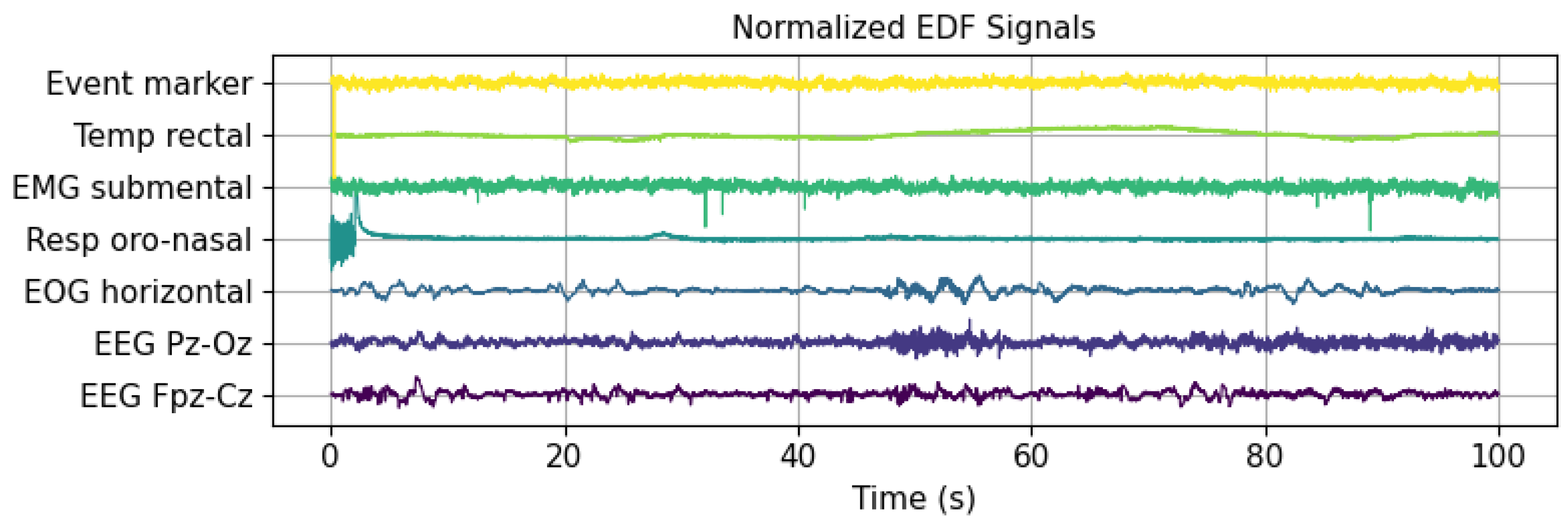Figure 1 illustrates the first 100 s of several signals from a PSG recording in the publicly available Sleep EDF Expanded database, utilized in this research. This database includes various signals, such as event markers, temperature, EMG, respiration, EOG, and two EEG channels. 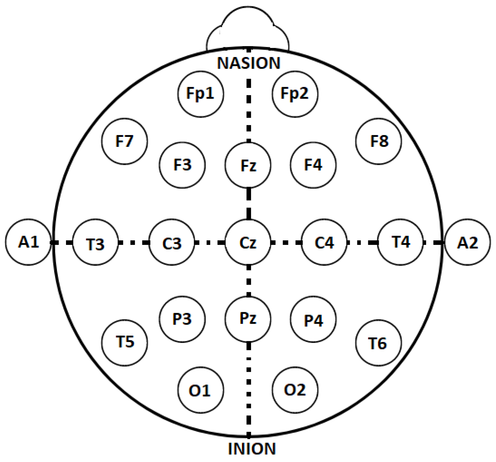The latter were recorded at different cortical locations after the international 10–20 electrode placement standard for EEG (Figure 2). The 10–20 placement protocol divides the cortex into areas based on the main brain lobes, assigning each a combination of letters and numbers. Fp, F, C, P, T, O, and A correspond to the frontal polar, frontal central, parietal, temporal, occipital, and auricular regions, respectively [15]. Even and odd numbers refer to the right and left brain hemispheres, respectively, while the letter z designates the central region of each lobe.

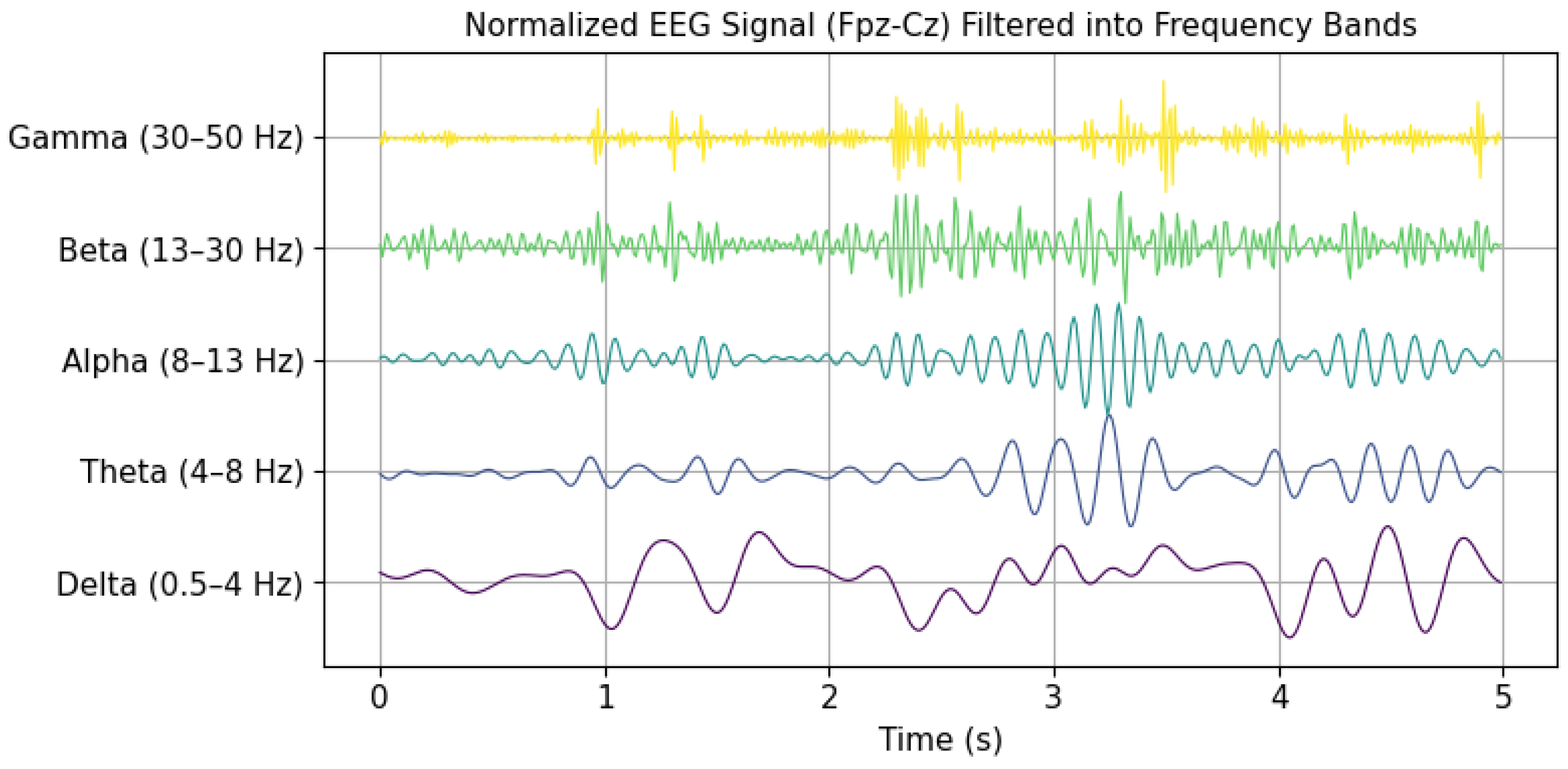
Information for the analysis of brain activity during sleep is obtained through EEG recordings. These signals are characterized by their non-linear, nonstationary, and often random nature, with voltage amplitudes ranging from 5 $\mathsf{\mu }$V to $200\mathsf{\mu }$V [16]. EEG signals are classified into five main wave types, varying in frequency from 0.5 to 128 Hz, and are identified by Greek letters: gamma (30–128 Hz), beta (13–30 Hz), alpha (8–13 Hz), theta (4–8 Hz), and delta (0.5–4 Hz) [12]. Figure 3 presents a temporal representation of brain waves over a 5 s interval. These waves were extracted from a signal within the Sleep EDF Expanded database. In this case, gamma wave activity above 50 Hz was discarded due to the 100 Hz sampling frequency, in accordance with the Nyquist criterion. Electrical patterns captured by EEG, such as variations in amplitude, frequency, and waveform morphology, are key indicators in identifying and characterizing different stages of sleep.

The first set of rules for categorizing sleep stages was introduced by Rechtchaffen and Kales in 1968, known as the R&K rules [17]. These rules define a sleep cycle with a duration between 90 and 110 min, comprising wakefulness (W), rapid eye movement (REM, hereafter referred to as R) sleep, and non-REM (NREM) sleep stages. The NREM phase consists of four distinct stages: S1, S2, S3, and S4. Sleep stages are typically assessed in 30 s intervals. In

Table 1. R&K rules for sleep stage classification.

Sleep Stage	Classification Criteria
W	This stage represents an alert state with high-level activity in the brain. EEG recordings display alpha waves (8–13 Hz, 20–40 $\mathsf{\mu }$V), commonly related to relaxation, and beta waves (13–30 Hz, 10–30 $\mathsf{\mu }$V), linked to cognitive and physical activity.
R	This stage is characterized by rapid eye movement beneath closed eyelids. The EEG exhibits a low-amplitude mix of theta and delta waves (2–7 Hz), and EMG activity in the chin decreases, leading to temporary muscle paralysis. During this stage, memory consolidation and emotional processing occur. Furthermore, REM sleep cycles last between 5 and 30 min per occurrence.
S1	This is an intermediate stage from wakefulness to sleep. It is defined by a decrease in alpha waves below 50% of the epoch, an increase in theta and delta waves (2–7 Hz), and slow rolling eye movements observed in EOG. This stage usually lasts between 5 and 10 min.
S2	This stage represents roughly 50% of the overall sleep duration and is classified as light sleep. It is characterized by the predominant theta activity (>75 $\mathsf{\mu }$V, <2 Hz), including both sleep spindles and K-complex patterns (>0.5 s), along with a notable decrease in both muscular engagement and eye activity.
S3	In this stage, deep sleep begins, with the predominance of delta waves (1–3 Hz, >75 $\mathsf{\mu }$V) of less than 50% of the epochs, although spindle bursts and K-complex waveforms can still appear. During this stage, physical and mental recovery processes take place.
S4	Also classified as deep sleep, this stage is predominantly composed of delta waves. Cardiac and respiratory rates decrease to their lowest levels, supporting immune function and muscle restoration.

, each sleep stage with its physiological characteristics is presented [17].

In 2007, the AASM revised the classification system to improve its clinical applicability. The update merged states S3 and S4 into a unified stage, designated N3, while stages S1 and S2 were changed to N1 and N2, respectively. Furthermore, the wakefulness stage was renamed wake [18,19].

This research presents a deep neural network framework for the classification of sleep stages using EEG data. Following the AASM guidelines, the classification targets the five main sleep stages: W, R, N1, N2, and N3. To address class imbalance, random undersampling at the epoch level is applied. The proposed architecture integrates convolutional neural networks (CNN) and bidirectional long short-term memory (BiLSTM) networks, further enhanced by an attention mechanism. This approach aims to eliminate the need for hand-crafted feature design and to enable the processing of extensive amounts of EEG data.

The methodology follows a structured pipeline consisting of five key steps: data acquisition and preprocessing, data splitting, class balancing, model training, and performance evaluation. Initially, EEG signals are obtained from PSG data along with the corresponding annotations from hypnogram (HYP) files. The signals then undergo preprocessing steps. Subsequently, the dataset is randomly partitioned into training, validation, and testing subsets. To address class imbalance, this work proposes an epoch-level random undersampling (E-LRUS) technique, applied to the training and validation sets. In the model training phase, deep learning architectures, specifically CNNs in combination with BiLSTM, are implemented to learn features directly from the EEG signals. In addition, an attention mechanism is integrated into the architecture to assign varying importance to different time steps. Finally, the trained models are evaluated using standard machine learning metrics to assess the classification performance.

Some contributions of this study include (1) the application of E-LRUS to address class imbalance across the training and validation sets; (2) the use of a hybrid deep learning architecture combining convolutional neural networks and bidirectional long short-term memory layers, enabling the extraction of both spatial and temporal features from raw EEG data; (3) the incorporation of an attention-based strategy that enhances the model’s ability to prioritize the most informative segments within each EEG sequence; (4) the development of a full deep learning pipeline that avoids manual feature engineering, supporting scalability and the efficient processing of large EEG datasets; and (5) the use of the publicly available Sleep-EDF Expanded dataset, promoting reproducibility and enabling direct benchmarking against existing approaches.

The remainder of this paper is structured as follows: Section 1 introduces the study; Section 2 discusses related works; Section 3 explains the developed methodology; Section 4 includes the data, experimental findings, and analysis; and, finally, Section 5 summarizes the conclusions and outlines possible future research.

2. Related Works

Classifying sleep stages using PSG recordings has been the objective of considerable research. Several works focus on EEG signals, as they provide valuable frequency-based insights into brain function in all stages of sleep. These signals, being one-dimensional, also offer the advantage of reducing the computational complexity compared to multimodal approaches, making them especially attractive for both clinical and computational applications. Most recent approaches leverage these EEG signals through machine learning or deep learning techniques, often reporting standard performance metrics such as accuracy or F1-scores on epoch-based datasets.

Many studies have used feature extraction in combination with classical classification algorithms. A notable early study by Doroshenkov et al. [20] leveraged the temporal structure of EEG signals, incorporating a hidden Markov model (HMM) to model state transitions in sleep stages. This model was enhanced by extracting features by applying a fast Fourier transform (FFT) using a Hamming window, which led to accuracy of 61.08%. Another study, conducted by Vural and Yildiz [21], assessed various EEG-derived features for the classification of the sleep stage. Their methodology included temporal features such as the mean value, standard deviation, and Hjorth parameter, along with frequency-based attributes such as the relative spectral power, spectral centroid, and spectral bandwidth. In addition, they incorporated time–frequency characteristics by combining both domains. Using principal component analysis (PCA) as a dimension reduction method, they achieved accuracy of 69.98%. Focusing on efficient classification, Huang et al. [22] proposed a low-computational-cost system designed for implementation in portable sleep monitoring devices. Their method used power spectral density (PSD) features obtained through a short-time Fourier transform (STFT) with a window overlapped in 0.5 s. To optimize feature selection, they applied prototype space feature extraction (PSFE) with fuzzy C-Means (FCM) clustering, alongside reduction methods including linear discriminant analysis (LDA) and PCA. Then, a support vector machine (SVM) was employed in the classification using a radial basis function (RBF) kernel, which produced accuracy of 70.92%. Other researchers have explored alternative classification strategies. Sanders et al. [23] focused on EEG-based spectral analysis, extracting features such as cross-frequency coupling (CFC) and spectral power across the delta, theta, alpha, beta, and gamma bands. Their approach used a continuous wavelet transform (CWT) with a Morlet wavelet to analyze phase–amplitude coupling, and classification was performed using LDA with cross-validation, resulting in accuracy of 75%. To further improve the classification accuracy, Nateghi et al. [24] introduced a novel approach using a Kalman time-varying autoregressive filter (TVAR) for feature extraction. Their classification process was divided into two steps: first, distinguishing between the stages W, REM, and non-REM, followed by refining the classification of the NREM substages (N1, N2, and N3). Using LightGBM and XGBoost classifiers, their system achieved accuracy that exceeded 77% with an average F1-score of 69%. Clustering-based methodologies have also been explored. Shuyuan et al. [25] proposed an improved K-Means clustering algorithm for EEG data segmentation. Unlike traditional K-Means, their method selected cluster centers based on the point density, addressing issues like initialization sensitivity and outliers. The cluster centroids were refined using the “Three Sigma Rule” during iterations, leading to classification accuracy of 75% in five sleep stages. Herrera [26], who used self-organizing maps (SOM) to create a structured EEG feature space, presented an alternative representation-based technique. This method was complemented by a feature selection process using mutual information (MI) criteria, which identified the most relevant variables for classification. Using an SVM with an RBF kernel and hyperparameter tuning via cross-validation, this approach yielded a classification accuracy score of 70.43%.

Recent advances in deep learning have significantly improved the sleep stage classification performance. Unlike traditional methods that rely on manually crafted features, deep learning models can automatically extract relevant patterns from raw EEG signals [27]. One of the first CNN-based approaches was introduced by Tsinalis et al. [5], who designed a convolutional neural network for the classification of sleep stages using single-channel EEG data. Their architecture consisted of a pair of convolutional layers that incorporated a pooling function, connected to dense layers, and a softmax classifier. They employed rectified linear activation functions and used a cross-entropy loss criterion. The EEG signals were preprocessed using wavelet analysis, and class balancing was achieved through stochastic gradient descent with weighted sampling. Their model achieved accuracy of 74%. More advanced CNN architectures have been developed since then. Sors et al. [7] proposed a CNN model that classified 30 s EEG epochs while incorporating contextual information from neighboring epochs. The training process used the ADAM optimizer with a data distribution of training (50%), validation (20%), and testing (30%). Their system demonstrated high accuracy of 87%. Hybrid deep learning models have also gained traction in sleep stage classification. Yang et al. [28] developed a nine-layer CNN-BiLSTM architecture that combined convolutional layers for feature extraction, BiLSTM layers for temporal modeling, and residual connections. Given the unbalanced distribution of data between categories of sleep, they implemented adaptive learning rate adjustments to avoid overfitting in the CNN layers. In addition, gradient clipping was applied in the BiLSTM layers to stabilize the training. The model achieved accuracy of 84.1%. Another hybrid model, SleepEEGNet, was proposed by Mousavi et al. [29]. The architecture combined CNN layers with BiLSTM layers that functioned as both encoders and decoders. Their system reached 84.26% precision, an F1-score of 79.66%, and a Cohen’s kappa coefficient of 0.79. Similarly, Toma et al. [30] introduced a multichannel CNN-BiLSTM model that integrated EEG (Fpz-Cz, Pz-Oz), EOG, and EMG signals. Their two-stage design leveraged pretrained dual-channel modules combined via transfer learning. The architecture reported accuracy of 91.44% with an F1-score of 88.69% using the Sleep-EDF 20 dataset, as well as accuracy of 90.21% over the extended Sleep-EDF 78 version.

Despite these improvements, certain challenges remain in classifying sleep stages, including the difficulty in accurately identifying stage N1, which is often underrepresented in datasets due to its short duration within the sleep cycle, and issues related to class imbalance. However, the ongoing development of deep learning methodologies and feature engineering strategies has contributed to increased classification accuracy. The use of models of hybrid neural networks and advanced preprocessing techniques suggests promising directions for the construction of improved models for the detection of sleep stages.

3. Methodology

The methodology of this research for the classification of sleep stages from EEG signals is based on a classic deep learning pipeline consisting of five steps: data acquisition and preprocessing, data splitting, class balancing, model training, and performance evaluation. Initially, EEG signals are extracted from PSG records and the corresponding sleep stage annotations are retrieved from the associated hypnogram (HYP) files. Subsequently, preprocessing and filtering are applied to the data to enhance the quality. The data are split into training, validation, and testing subsets to assess model training and evaluation. To handle imbalance issues among classes, this work introduces a random undersampling method, which is applied at the epoch level, specifically targeting the training and validation sets. Afterward, several neural network architectures, including a CNN, BiLSTM, and the attention mechanism in combination, are trained, validated, and tested in the subsets. Performance is measured based on several metrics, such as accuracy, the F1-score, and Cohen’s kappa, among others. The procedural steps are outlined in the diagram in Figure 4. The following sections provide a detailed analysis of each step of the methodology, along with their theoretical foundations.

3.1. Data Acquisition and Preprocessing

The EEG signals used in this study are selected from PSG recordings stored in European Data Format (EDF) files [31], a widely adopted standard for the storage of biomedical data. These files contain both physiological signals and relevant metadata, including the sampling rate, signal characteristics, and patient information [32]. First, the EEG signals are extracted from the PSG files, and the associated sleep stage annotations are obtained from the corresponding HYP files [33]. These annotations denote the different stages of sleep, such as W, R, S1, S2, S3, and S4, typically labeled in 30 s intervals. The extracted data are then organized into a matrix in which each temporal sample is associated with its corresponding EEG signal and the sleep stage label. Several conditioning steps are applied to align with the AASM guidelines for the classification of sleep stages [18]. As a result, the final sleep stages used for classification are N1, N2, N3, R, and W. Since sleep stages are represented as categorical labels, these labels are converted using ordinal label encoding, assigning a unique integer to each stage [34].

In addition, the signals are normalized to ensure consistency between different subjects and recordings. Min–max normalization is employed to scale each sample $x_i$ of the EEG signal to a uniform range, typically [0, 1] [35]:

$$x_i^{\prime }={\displaystyle \frac{x_i-x_{\min }}{x_{\max }-x_{\min }}},$$

(1)

where $x_i$ is the original EEG sample; $x_{\min }$ and $x_{\max }$ are the minimum and maximum values of the signal within the recording, respectively; and $x_i^{\prime }$ is the normalized value. This normalization standardizes the signal scales across individuals and constitutes the only preprocessing step applied, in order to avoid extensive feature engineering and to preserve the raw signal input. By minimizing intermediate transformations, this approach aims to retain the intrinsic structure of the signals and enable direct feature learning.

3.2. Data Splitting

The dataset split plays a fundamental role in the development of a reliable model, ensuring adequate learning from the data and generalization to unseen data. Typically, datasets are divided into three subsets—training, validation, and testing [34]—which split the data as follows.

• Training Set (60%): Utilized for fitting the model’s weights. It must be large enough to capture the data’s patterns and complexity.
• Validation Set (20%): Applied for hyperparameter tuning and intermediate evaluation.
• Test Set (20%): Reserved for the final assessment, it provides an unbiased measure of the generalization capability of the model.

This method of dividing the data allows good performance in both training data and new unseen data during testing.

3.3. Class Balancing

Class imbalance can affect model quality and generalization, particularly in supervised classification tasks. When certain classes have significantly more samples than others, models tend to bias their predictions towards the majority class, leading to reduced performance in minority classes [36]. Although there are various class-balancing techniques to address this issue, special care must be taken when dealing with temporal models such as LSTM. Common techniques like random oversampling or undersampling at the sample level can break temporal coherence, thus affecting the model’s ability to learn long-term patterns [37]. Other techniques, such as the synthetic minority oversampling technique (SMOTE), are not suitable because they generate synthetic samples that alter sequences, compromising temporal relations [38]. To overcome this, we introduce an epoch-level random undersampling (E-LRUS) technique that preserves the sequential structure of the data. E-LRUS operates by randomly removing entire epochs from the majority classes while maintaining the continuity of the original sequence. Since the EEG signals in PSG are annotated every 30 s, the segments are treated as single epochs and assigned unique indices to retain their original temporal order. The epochs are grouped by class, and the class with the fewest epochs is identified. For each of the remaining classes, a subset of epochs equal in number to that of the minority class is randomly selected, and the rest are discarded. After the undersampling process, the selected epochs of all classes are recombined and reordered according to their original temporal indices. Mathematically, the E-LRUS algorithm is presented below. Considering a sequence set X,

$$X=(x_i,y_i)|x_i\in {\mathbb{R}}^d,y_i\in 1,2,\dots ,C,$$

(2)

where $x_i$ denotes the i-th sample within the data collection, which, in this case, is a scalar value ($d=1$), and $y_i$ denotes the label of the sample, which belongs to one of the C total classes. The data are divided into epochs $E_j$ of fixed duration T. For a sampling frequency $f_s$, the number of samples per epoch is $N_s$$N_s=T·f_s$. Then, each epoch is defined as

$$E_j=\{x_k\mid n_k\in [n_j,n_j+N_s)\},$$

(3)

where $x_k$ represents the k-th sample in the dataset, $n_k$ is the sequence position in the time series, and $n_j$ is the starting index of epoch j. The total epoch number for any class c is given by $N_c$. The minority class is defined as

$$N_{\min }=\underset{c\in \{1,\dots ,C\}}{\min }{N}_c.$$

(4)

For each class c with $N_c>N_{\min }$, we randomly select $N_{\min }$ epochs in the following way:

$$E_c^{\prime }\subset E_c,\mathrm{with}\left|E_c^{\prime }\right|=N_{\min },$$

(5)

where $E_c$ is the set of epochs for class c, and $E_c^{\prime }$ is the subset of $N_{\min }$ epochs selected randomly. Therefore, the selected epochs are

$$E_c^{\prime }=\{E_j\mid E_j\in E_c,j\in S_c\},$$

(6)

where $S_c$ is a random subset of indices from $E_c$, and $E_j$ is the j-th epoch from $E_c$. The final balanced set is denoted as

$$X^{\prime }=\bigcup _{c=1}^C{E}_c^{\prime }.$$

(7)

This approach preserves the temporal coherence, reduces the dataset size, and ensures effective learning for temporal models like LSTM without disrupting the order of the sequences.

3.4. Model Training

Machine learning develops algorithms that learn patterns from data to perform tasks such as classification, regression, and clustering [39]. In deep learning, neural networks are algorithms inspired by the structure of the brain [40,41], designed to recognize these patterns and learn complex relationships. A neural network consists of layers of artificial neurons, where each neuron processes inputs through a weighted sum followed by an activation function, which can be expressed as

$$a=f\left(z\right)=f\left(\sum _{i=1}^n{w}_i{x}_i+b\right),$$

(8)

where $x_i$ denotes the inputs, $w_i$ denotes weight vectors, b is the bias, z is the weighted sum, $f(·)$ is the activation function, and a is the output of the neuron [42]. Figure 5 provides a visual representation of the internal components of an artificial neuron.

Non-linearity is introduced into the model through activation functions. Among the principal activation functions are the sigmoid ($\sigma$), hyperbolic tangent (tanh), rectified linear unit (ReLU), and softmax functions. These functions are described in

Table 2. Classification results of the best model on the validation set.

Activation	Function	Description
Sigmoid	$\sigma \left(z\right)={\displaystyle \frac{1}{1+e^{-z}}}$	In binary classification, it maps real values to the range [0, 1] [42].
Tanh	$\tanh \left(z\right)={\displaystyle \frac{e^z-e^{-z}}{e^z+e^{-z}}}$	Transforms inputs to outputs between −1 and 1 [42].
ReLU	$\mathrm{ReLU}\left(z\right)=\max (0,z)$	Outputs the input if it is greater than zero; otherwise, it is zero [43].
Softmax	$\mathrm{Softmax}\left(z_i\right)={\displaystyle \frac{e^{z_i}}{{\sum }_{j=1}^n{e}^{z_j}}}$	Converts a vector of values into probabilities, where $z_i$ and $z_j$ are the weighted sums for classes i and j, respectively. This function is particularly useful for multiclass classification tasks [40].

.

The structure of a neural network includes an input layer, hidden layers, and an output layer [40], as shown in Figure 6. The raw input data are fed into the network through the input layer, with each neuron corresponding to an individual feature. Neurons within the hidden layers transform signals from the preceding layer through activation functions. Predictions are generated in the output layer, which typically employs activation functions that map the output into a probabilistic interpretation.

Training a neural network involves adjusting the weights $w_i$ and biases b to minimize the error between the predicted and actual outputs [44]. This process is carried out iteratively through the following stages: forward propagation, evaluation via loss functions, backpropagation, and parameter adjustment using optimization algorithms. Regularization techniques are often applied to prevent overfitting and improve the generalization performance. Moreover, the design of a neural network is influenced by factors such as the number of layers, the arrangement of neurons, and the type of layer used. The following sections outline the stages involved in training a neural network, including forward propagation, loss functions, backpropagation, optimization, and regularization strategies. Subsequently, different types of neural network layers are reviewed.

3.4.1. Forward Propagation

Forward propagation involves passing the input $x_i$ through the network layers to generate an output $\widehat{y}$ [40]. It is the process of making predictions, where the data flow through the layers and transformations are applied. At layer l, the output is computed as

$$a^{\left(l\right)}=f\left(z^{\left(l\right)}\right)=f\left(\sum _{i=1}^n{w}_i^{\left(l\right)}{x}_i^{(l-1)}+b^{\left(l\right)}\right),$$

(9)

with the final output being

$$\widehat{y}=a^{\left(L\right)},$$

(10)

where L represents the last layer of the network.

3.4.2. Loss Function

The loss function serves to evaluate the discrepancy between the predicted value $\widehat{y}$ and the corresponding ground truth label y. For regression tasks, the mean squared error (MSE) is typically used [45]:

$$J_{\mathrm{MSE}}={\displaystyle \frac{1}{m}}\sum _{i=1}^m{(y_i-{\widehat{y}}_i)}^2,$$

(11)

where m is the number of training examples. In classification tasks, the cross-entropy (CE) loss is often utilized to compare the predicted probability distribution with the actual class labels. In binary classification, the CE loss is defined as [45]

$$J_{\mathrm{CE}}=-{\displaystyle \frac{1}{m}}\sum _{i=1}^m\left[y_i\log \left({\widehat{y}}_i\right)+(1-y_i)\log (1-{\widehat{y}}_i)\right].$$

(12)

When dealing with multiclass classification involving C distinct categories, the CE loss generalizes to

$$J_{\mathrm{CE}}=-{\displaystyle \frac{1}{m}}\sum _{i=1}^m\sum _{j=1}^C{y}_{ij}\log \left({\widehat{y}}_{ij}\right),$$

(13)

where $y_{ij}$ is a binary value indicating whether instance i belongs to class j (1 if true, 0 otherwise), and ${\widehat{y}}_{ij}$ denotes the model’s estimated probability that instance i is assigned to class j.

3.4.3. Backpropagation

To minimize errors, the weights and biases of the network are updated using the loss function gradients $J(W,b)$ in a process called backpropagation [46]. In this process, the error flows from the output layer back toward the input layer, and the gradients are computed to update the model parameters via optimization algorithms such as gradient descent (GD):

$$w^{\left(l\right)}=w^{\left(l\right)}-\eta {\displaystyle \frac{\partial J(W,b)}{\partial w^{\left(l\right)}}},b^{\left(l\right)}=b^{\left(l\right)}-\eta {\displaystyle \frac{\partial J(W,b)}{\partial b^{\left(l\right)}}},$$

(14)

where $\eta$ is the learning rate, and W represents the collection of all weight parameters in the network. The gradient computation follows the chain rule as follows:

$${\displaystyle \frac{\partial J(W,b)}{\partial w^{\left(l\right)}}}={\displaystyle \frac{\partial J}{\partial a^{\left(L\right)}}}{\displaystyle \frac{\partial a^{\left(L\right)}}{\partial z^{\left(L\right)}}}{\displaystyle \frac{\partial z^{\left(L\right)}}{\partial w^{\left(l\right)}}},$$

(15)

where each term is the derivative at a different layer. The error at layer l is given by

$${\delta }^{\left(l\right)}={\displaystyle \frac{\partial J(W,b)}{\partial z^{\left(l\right)}}},$$

(16)

which propagates backward as

$${\delta }^{\left(l\right)}={\left(W^{(l+1)}\right)}^T{\delta }^{(l+1)}\odot f^{\prime }\left(z^{\left(l\right)}\right),$$

(17)

where ⊙ denotes the Hadamard product. Finally, the weight and bias gradients are

$${\displaystyle \frac{\partial J(W,b)}{\partial w^{\left(l\right)}}}={\delta }^{\left(l\right)}{\left(a^{(l-1)}\right)}^T,{\displaystyle \frac{\partial J(W,b)}{\partial b^{\left(l\right)}}}=\sum _{i=1}^m{\delta }_i^{\left(l\right)}.$$

(18)

The resulting gradients are applied in successive iterations to update the weights of the network, gradually improving the predictive performance of the model.

3.4.4. Parameter Optimization

Optimization methods such as stochastic gradient descent, root mean square propagation, and adaptive moment estimation improve the efficiency of the model learning process beyond standard GD.

• Stochastic Gradient Descent (SGD): Updates weights using a random sample per iteration [47], reducing the complexity; efficient in large datasets.
• Root Mean Square Propagation (RMSProp): Modifies the learning rate dynamically by tracking the moving mean value of squared gradients [48], accelerating convergence.
• Adaptive Moment Estimation (ADAM): Integrates momentum and learning rate adaptation [48], using decaying averages of past gradients for faster and stable convergence.

The optimization choice depends principally on the task, the data, and the hyperparameters.

3.4.5. Regularization

Regularization techniques reduce overfitting and improve the ability of a model to generalize to unseen data [49]. Among the most widely used are the following.

• Dropout: This technique randomly turns off subsets of neurons during each training iteration [50], reducing the dependence on individual neurons.
• L2 Regularization: This technique penalizes large weights to reduce overfitting [51], minimizing the prediction error and weight size. A penalty is introduced into the cost function, scaling with the total of weight squares.
• Early Stopping: This method works by tracking the validation performance during training [52], which is stopped if the validation loss is not progressing or degrading, preventing overfitting and unnecessary iterations.
• Batch Normalization: This method normalizes layer activation, ensuring a standard normal distribution for activation values within each mini-batch [53]. This approach improves convergence, mitigates internal covariate shifts, and acts as a regularizer [4].

The effectiveness of these strategies varies based on the model structure and the nature of the data; they contribute to better generalization and improved performance.

3.4.6. Fully Connected Layers

Fully connected (FC) layers are a fundamental component in neural network architectures. In these layers, each neuron is connected to every neuron in the subsequent layer [54], allowing the model to learn complex and high-dimensional representations of features. The operation of a fully connected neuron is defined as

$$y=f\left(\sum _{i=1}^n{w}_i{x}_i+b\right),$$

(19)

where $w_i$ denotes each weight, $x_i$ represents the corresponding input, b is the bias, $f(·)$ refers to the activation function, and n indicates the total number of inputs. This formulation describes the elementary function executed by a single neuron. For a layer comprising m neurons, the computational complexity is $\mathcal{O}(m·n)$, making FC layers computationally expensive for large-scale applications. Furthermore, FC layers are typically used in the final stages of a network for the aggregation and classification of features [40].

3.4.7. Convolutional Layers

Convolutional neural networks are designed to process structured data [55] through convolutional operations, where learnable filters slide across the input to capture local features [56]. The convolution operation in discrete time for a 1D input is defined as [57]

$$y\left(n\right)=(x\ast w)\left(n\right)=\sum _{k=0}^{K-1}w\left(k\right)·x(n-k),$$

(20)

where $x\left(n\right)$ is the input sequence at index n, $w\left(k\right)$ is the filter kernel at index k, and K is the number of coefficients in the filter kernel. When considering stride s and padding P, the convolution operation is adjusted as follows:

$$y\left(n\right)=\sum _{k=0}^{K-1}w\left(k\right)·x(n·s+k-P),$$

(21)

where s denotes the step size of the moving window filter, and P represents the number of zeros added around the input to maintain the size [58]. A 1D convolutional layer involves $\mathcal{O}(N·K·C_{\mathrm{in}}·C_{\mathrm{out}})$ operations, where $C_{\mathrm{in}}$ and $C_{\mathrm{out}}$ denote the channel dimensions before and after convolution, respectively. To further reduce the computational load and control overfitting, CNN architectures commonly employ pooling operations. The scheme of Figure 7 shows the layered structure of a CNN.

The operation of combining layers downsamples the sizes of feature maps by summarizing local regions [59]. Two widely used pooling strategies are maximum pooling, which retains the maximum value found in a size window K, highlighting the dominant features of the signal, and average pooling, which smooths the data by averaging the values across a sequence.

In CNNs, filters, also known as kernels, are trainable parameters optimized through backpropagation. These filters function similarly to finite impulse response filters (FIRs), modifying the signal by enhancing or attenuating specific patterns [60]. The convolution in the frequency domain can be represented by the multiplication of Fourier transforms [57]:

$$Y\left(f\right)=X\left(f\right)·W\left(f\right),$$

(22)

where $X\left(f\right)$, $W\left(f\right)$, and $Y\left(f\right)$ are the Fourier transforms of the input, filter, and output, respectively. This relationship highlights how convolutional filters can enhance or suppress specific frequency components of the input signal [61]. By directly extracting these filters from the data, CNNs provide a framework capable of adapting to various input types.

3.4.8. LSTM Layers

Long short-term memory (LSTM) networks are variants of traditional recurrent neural networks (RNNs) that addresses vanishing and exploding gradient issues [62]. Unlike standard RNNs, LSTM models include internal gates, namely input, forget, and output gates, designed to control which data are stored, discarded, or passed on. This architecture makes LSTM particularly suitable for complex sequence tasks such as text analysis, machine translation, and time-series forecasting [63]. In an LSTM layer, several parallel cells manage different elements of the sequential input. At each time step t, the memory state $C_t$ updates according to [64]

$$C_t=f_t{C}_{t-1}+i_t{\tilde{C}}_t,$$

(23)

where $f_t$, $i_t$, and ${\tilde{C}}_t$ correspond to the forget gate, input gate, and candidate memory content, respectively. These components are computed internally within each LSTM cell through a specific operation [8]. The forget gate regulates the amount of historical data to retain:

$$f_t=\sigma (W_f[h_{t-1},x_t]+b_f),$$

(24)

where $W_f$ represents the weight parameters linked to the forget gate, $h_{t-1}$ is the hidden state from the last time step, $x_t$ indicates the current input, $b_f$ is the bias for the forget gate, and $\sigma$ is the sigmoid function that produces output values between 0 and 1. Similarly, the input gate determines the amount of new information to be stored in the cell state:

$$i_t=\sigma (W_i[h_{t-1},x_t]+b_i),$$

(25)

where $W_i$ denotes the weights and $b_i$ is the bias associated with the input gate. The candidate memory content, which proposes possible modifications to the cell state, is computed as

$${\tilde{C}}_t=\tanh (W_C[h_{t-1},x_t]+b_C),$$

(26)

where $W_C$ and $b_C$ are the respective weights and bias for the candidate memory. The use of tanh allows the regulation of values in the range $[-1,1]$, introduces variability, and captures positive and negative influences on the state of the memory. The output gate regulates the impact of the stored memory on the hidden state:

$$o_t=\sigma (W_o[h_{t-1},x_t]+b_o),$$

(27)

with $W_o$ and $b_o$ representing the weights and bias linked to the output gate. Finally, the hidden state $h_t$ is updated during each time step according to the output gate and the current memory state:

$$h_t=o_t\tanh \left(C_t\right).$$

(28)

The overall architecture of an LSTM cell is shown in Figure 8.

Each gate operation involves matrix multiplications of size $d\times (d+n)$, which leads to a computational cost per step of $\mathcal{O}(d·n)$. Consequently, processing a sequence of length T across L stacked layers leads to an overall computational cost of $\mathcal{O}\left(T{\sum }_{l=1}^L{d}_{l}n\right)$ [65], highlighting the importance of optimizing LSTM architectures to meet hardware constraints.

An extension of LSTM is BiLSTM, which processes sequences in both forward and backward directions [9]. In a BiLSTM model, each time step t has two associated hidden states:

$$h_t^{\mathrm{BiLSTM}}=\left[\begin{array}{c}{h}_t^{\to }\\ h_t^{\leftarrow }\end{array}\right],$$

(29)

where $h_t^{\to }$ represents the hidden state moving forward through time, and $h_t^{\leftarrow }$ represents the hidden state moving backward [66]. The structure of BiLSTM is shown in Figure 9, where the resulting output $h_t$ of the primary LSTM layer is connected to the input of the secondary LSTM layer moving forward in time. This architecture allows the model to leverage contextual information from both past and future inputs, enhancing its sequence understanding [65].

Although BiLSTM significantly improves the performance by capturing information flowing in both temporal directions, it inherently doubles the memory usage and computational requirements compared to standard unidirectional LSTM. Therefore, its application must balance the benefits of enhanced context awareness with the increased computational cost.

3.4.9. Attention Layers

Attention mechanisms dynamically assign importance to different elements of a sequence, enhancing the performance in natural language processing (NLP), sequential modeling, and computer vision tasks [67]. Inspired by human cognition, they allow networks that concentrate attention on key segments of the input, boosting the learning efficiency and interpretability. Among the main attention networks are the following.

• Hard attention: Selects a single input position, making it non-differentiable [68]:

  $$\mathrm{HardAttention}(Q,K)=\mathrm{argmax}\left(Q{K}^T\right),$$

  (30)

  where Q and K are the query and key matrices, respectively. Since backpropagation is infeasible, alternative approximations are preferred.
• Soft attention: Assigns probabilistic weights to all input positions using the softmax function [69]:

  $$\mathrm{SoftAttention}(Q,K,V)=\mathrm{softmax}\left({\displaystyle \frac{Q{K}^T}{\sqrt{d_k}}}\right)V.$$

  (31)

  where V is the value matrix and $d_k$ is a scaling factor for numerical stability.
• Self-attention: A special case of soft attention where queries, keys, and values are derived from the same input [70]. In Figure 10, a diagram of the self-attention mechanism is shown.

Attention mechanisms are key in modern deep learning, enabling the handling of complex dependencies in large-scale data. In the proposed model, self-attention layers are placed after each BiLSTM block to dynamically weight temporal outputs and focus on the most informative segments of the EEG sequence.

3.5. Performance Evaluation

Once a classification model is trained, evaluating its effectiveness becomes essential to ensure its reliability and generalization. Various metrics can be used to quantify its predictive capability, offering a comprehensive evaluation [71].

• Confusion Matrix—A matrix of size $C\times C$, with C representing the total classes, and each entry $(i,j)$ represents instances of class i classified as j. This structure enables the computation of key metrics like accuracy, precision, recall, and the F1-score.
• Overall Accuracy—Represents the fraction of correctly classified samples:

  $$\mathrm{Accuracy}={\displaystyle \frac{TP+TN}{TP+TN+FP+FN}}.$$

  (32)

  with $TP$ indicating true positives, $TN$ true negatives, $FP$ false positives, and $FN$ false negatives.
• Precision—Evaluates how reliably positive cases are identified:

  $$\mathrm{Precision}={\displaystyle \frac{TP}{TP+FP}}.$$

  (33)
• Recall or Sensitivity—Measures how well the model identifies positive cases:

  $$\mathrm{Recall}={\displaystyle \frac{TP}{TP+FN}}.$$

  (34)
• Specificity—Evaluates the model’s ability to accurately identify negative cases:

  $$\mathrm{Specificity}={\displaystyle \frac{TN}{TN+FP}}.$$

  (35)
• Negative Predictive Value (NPV)—Indicates the proportion of correctly predicted negative cases among all predicted negatives:

  $$\mathrm{NPV}={\displaystyle \frac{TN}{TN+FN}}.$$

  (36)
• F1-Score—Integrates precision and recall into one measure, being particularly effective for imbalanced datasets:

  $$F1=2\times {\displaystyle \frac{\mathrm{Precision}\times \mathrm{Recall}}{\mathrm{Precision}+\mathrm{Recall}}}.$$

  (37)
• Jaccard Index or Intersection over Union—Quantifies the overlap between predicted and true positive instances:

  $$\mathrm{Jaccard}={\displaystyle \frac{TP}{TP+FP+FN}}.$$

  (38)
• Cohen’s Kappa Coefficient—Measures the consistency between predicted and true labels, adjusted for agreement by chance:

  $$\kappa ={\displaystyle \frac{P_o-P_e}{1-P_e}},P_o={\displaystyle \frac{TP+TN}{N}},P_e=\sum _{i=1}^k{\displaystyle \frac{T_i{P}_i}{N^2}}.$$

  (39)

Graphical evaluation also complements numerical metrics [70].

• Receiver Operating Characteristic (ROC) Curve: Displays the true positive rate against the false positive rate for different classification thresholds. A larger area under the curve (AUC) reflects improved classifier performance.
• Precision–Recall Curve: Especially useful for imbalanced datasets, this curve shows the trade-off between precision and recall.

Using multiple metrics provides a holistic view of model behavior and guides informed adjustments to the hyperparameters. These evaluations can quantify model performance and, furthermore, provide insights into practical strengths and limitations in real-world contexts.

4. Results and Discussion

In the context of implementing deep learning approaches for multiclass classification tasks, each decision significantly impacts the performance. Selecting a suitable sleep dataset for research, ensuring a computational environment capable of processing large amounts of raw data, and preprocessing signals are essential steps in this workflow. In addition, aspects related to the neural network, such as the parameter setup, architecture, training process, and performance evaluation metrics, are fundamental considerations that must be addressed and can be experimentally adjusted to optimize model performance. These considerations provide the foundation for optimizing the effectiveness of the model when evaluating sleep stage classification using EEG signals. To validate these considerations, the following experiments are presented.

4.1. Dataset

In this study, the Sleep-EDF Expanded Database is considered, which is widely recognized in EEG-based sleep research [72]. This dataset contains 197 full PSG recordings in EDF format, with multiple sessions from 78 subjects (healthy and with sleep disorders) between 25 and 101 years of age. These data were collected during approximately 20 consecutive hours of sleep monitoring in a home environment [33]. The recordings comprise several physiological signals: two EEG signals, EOG, submental EMG, event makers, respiration, and body temperature, all stored in EDF format with a 16-bit resolution. Each EDF file is accompanied by metadata, including patient information, recording settings, signal specifications, and administrative details. The EEG channels (Fpz-Cz and Pz-Oz) follow the 10–20 international system, covering the frontal and occipital regions, as suggested by the AASM. EEG and EOG signals were sampled at 100 Hz, while the remaining signals were sampled at 1 Hz [33]. The recordings are divided into 30 s epochs and each labeled according to the R&K guidelines as “W”, “1”, “2”, “3”, “4”, “R”, “movement”, and unlabeled segments.

4.2. Experimental Environment

Deploying deep learning architectures with raw EEG data requires significant computational resources. All experiments were carried out on a device equipped with a 13th-gen Intel Core i9-13900K processor (3.00 GHz), an Nvidia RTX 4070 GPU, and 16 GB RAM, running Windows 11 Pro 64-bit. The development environment included Python 3.9.0, using frameworks like PyTorch, NumPy, Scikit-learn, and PyEDFlib. Visualization was performed using Matplotlib V. 3.10.0 and Seaborn V. 0.13.2. This configuration provided the computational power necessary to carry out all the experiments presented in order to achieve the presented results.

4.3. Data Preprocessing

To ensure the consistency and relevance of the input data, several preprocessing steps were applied to the EEG recordings prior to model training. First, the Fpz-Cz EEG channel was extracted from each EDF file to adapt the input to a single-channel architecture, minimizing the complexity while preserving critical information for sleep stage classification. To improve the data quality and address class imbalance, only epochs with valid sleep stage annotations were retained. Epochs labeled “movement” or left unannotated were discarded entirely because they introduced noise and lacked ground truth. Furthermore, epochs labeled stage W were selectively retained only during transitional periods around the onset of sleep and awakening; this was done to avoid the overrepresentation of wakefulness and to balance the distribution between classes. According to the AASM guidelines, stages 3 and 4 were combined into the N3 category. The final class labels were then numerically encoded as follows: N1 = 0, N2 = 1, N3 = 2, R = 3, and W = 4. After class filtering and relabeling, all EEG signals were normalized to the range [0, 1] using min–max normalization. No additional artifact rejection or filtering was applied, following an end-to-end modeling strategy where the model learned directly from the raw normalized signal.

Regarding data organization, complete EDF files were stored per patient. The dataset was divided by assigning entire EDF files: 60% for training, 20% for validation, and 20% for testing. This prevented the split of files across subsets, ensuring full recordings per patient and a subject-independent evaluation. To address class imbalance, the E-LRUS technique was applied to the training and validation sets, promoting balanced learning and better model generalization. This preprocessing pipeline is designed to maintain data integrity, reduce bias, and enable robust subject-level evaluation, ensuring that the model is trained and tested under realistic and representative input conditions.

4.4. Proposed Neural Network Architecture

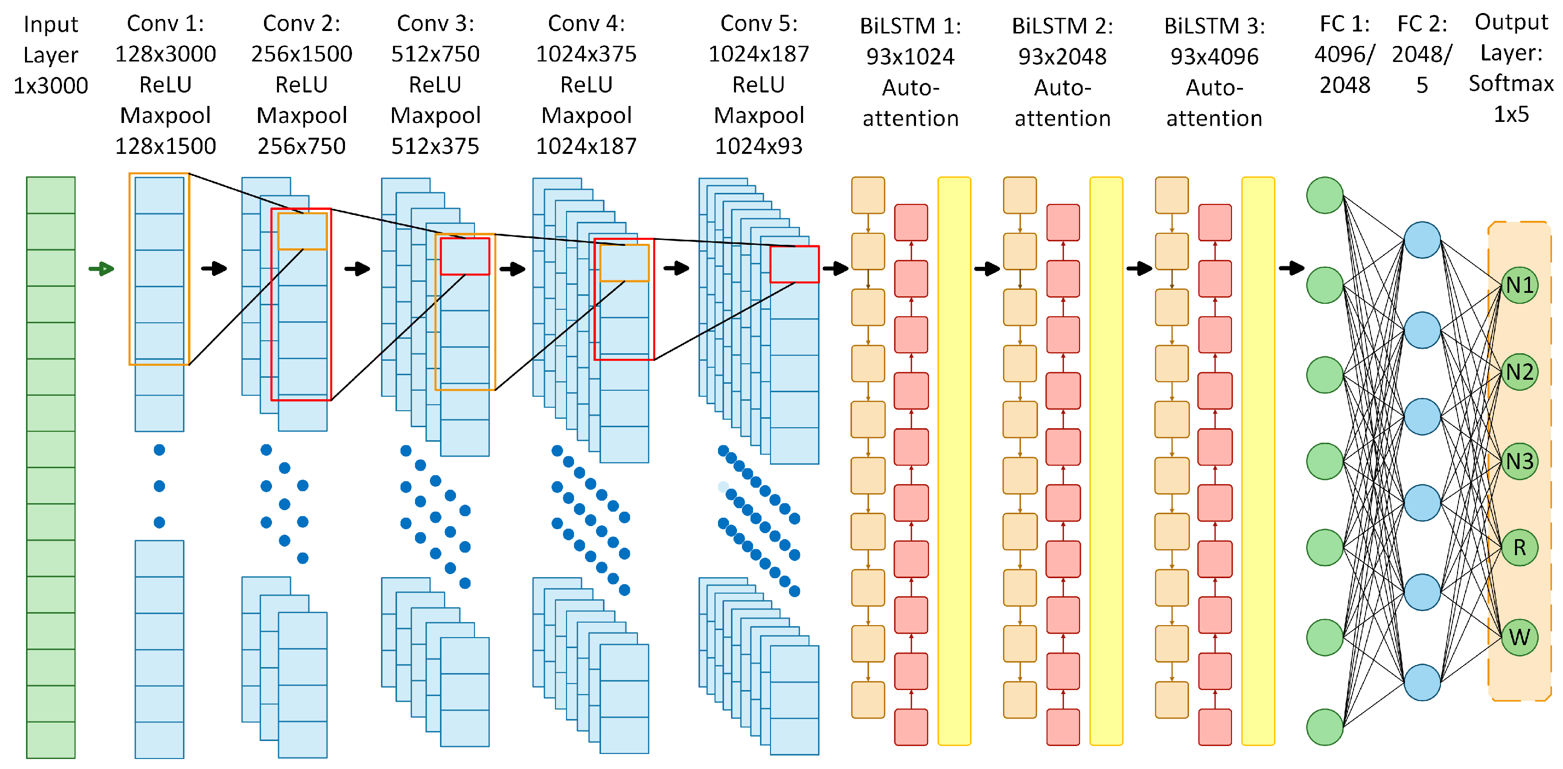
The proposed neural network architecture was designed to perform sleep stage classification in EEG recordings using a combination of CNNs, BiLSTM, and self-attention mechanisms. It consists of five main components.

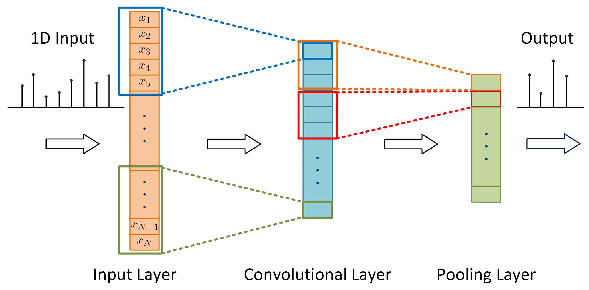
• 1D Convolutional Layers: Five layers with increasing filters (from 128 to 1024), each with ReLU activation, maximum pooling operations, and batch normalization. The choice of five layers adds depth to capture complex EEG features, while max pooling enables hierarchical extraction and dimensionality reduction, allowing the efficient processing of long sequences.
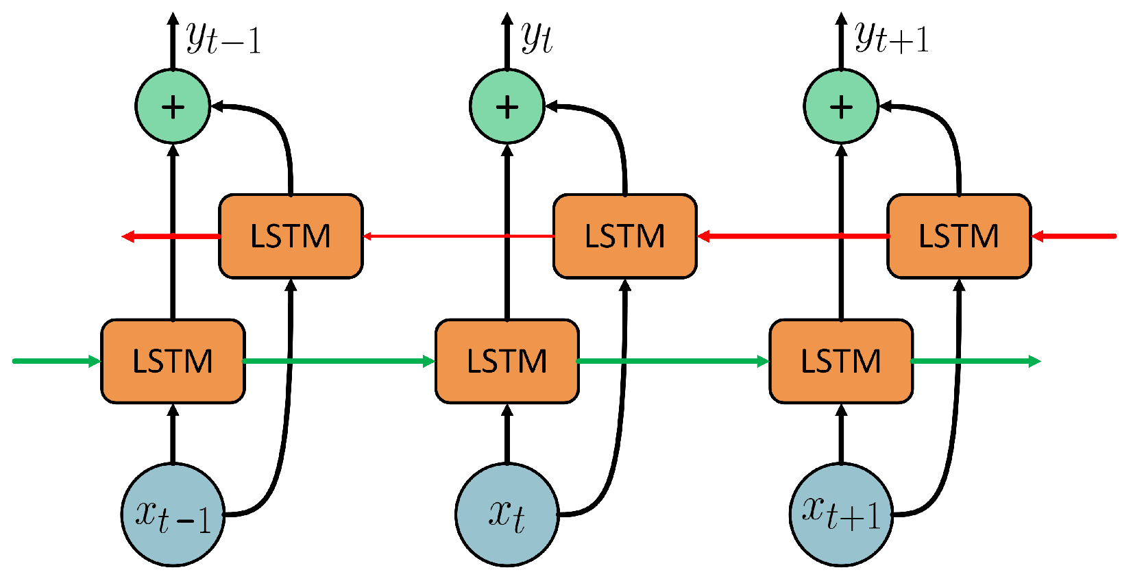
• Bidirectional LSTM Layers: Three BiLSTM layers with 512, 1024, and 2048 memory cells, respectively. The use of three layers helps to capture complex long-term temporal dependencies in both directions, supporting the modeling of the sequential nature of sleep stages.
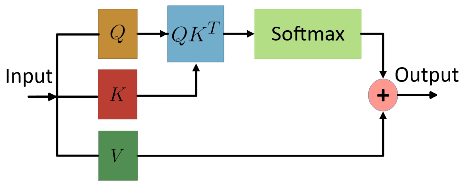
• Self-Attention Layers: Placed after each BiLSTM, these dynamically weight the hidden states over time. This allows the model to focus on the most relevant temporal features, complementing BiLSTM’s ability to capture dependencies and improving the discrimination of transient or subtle sleep stage patterns.
• Fully Connected Layers: Two dense layers with 2048 and 5 outputs, respectively, with ReLU activation. The first dense layer reduces the high-dimensional LSTM output to 2048 units for feature consolidation, while the second generates classification scores for the five sleep stages.
• Softmax Output Layer: A final softmax output layer that maps the outputs to probabilities for each of the five sleep stages: N1, N2, N3, R, and W.

The number of layers and units was empirically selected based on the validation performance in multiple configurations. Although increasing the complexity of the model generally improved the performance, the upper limit was constrained by the available computational resources. To efficiently process long EEG sequences and handle large volumes of data, the model leverages hierarchical convolutional feature extraction and max pooling to reduce the dimensionality. This reduction, combined with dense layers, enables scalability to extended recordings despite computational limitations. In addition, attention mechanisms were incorporated to explore their potential impact on the capture of important temporal features in EEG signals and to selectively emphasize informative EEG segments relevant to each stage of sleep. The scheme of the proposed model architecture is shown in Figure 11, which illustrates the arrangement of the layers involved in the learning process. This architecture yielded the best classification performance among several alternatives and was used in subsequent experiments.

4.5. Parameter Configuration

After completing data preprocessing and defining the architecture of the neural network, the model training process was carried out. The loss function used was the categorical cross-entropy, handling non-numeric classes probabilistically. The SGD, RMSprop, and ADAM optimizers were tested, with the latter yielding the best results. Since ADAM adjusts the learning rate automatically, it was not specified manually. In the context of regularization techniques, various dropout values between 0 and 1 were tested, and a value of 0.7 led to the best model performance. Furthermore, weight decay was applied using a penalty coefficient of $5·{10}^{-4}$. The signals were divided into 30 s sequences. For EEG signals sampled at 100 Hz, this is equal to 3000 samples per sequence. During the application of E-LRUS, the training set was balanced to 537 epochs per class, based on the least represented class, N1. Several batch sizes (16, 32, 64, and 128) were tested, with the best results achieved with 64 samples per batch. The learning cycles were set to a total of 100 epochs, with early stopping configured at 30 epochs. These parameters were fine-tuned across training sessions and corresponded to those that led to the best-performing model.

4.6. Network Training

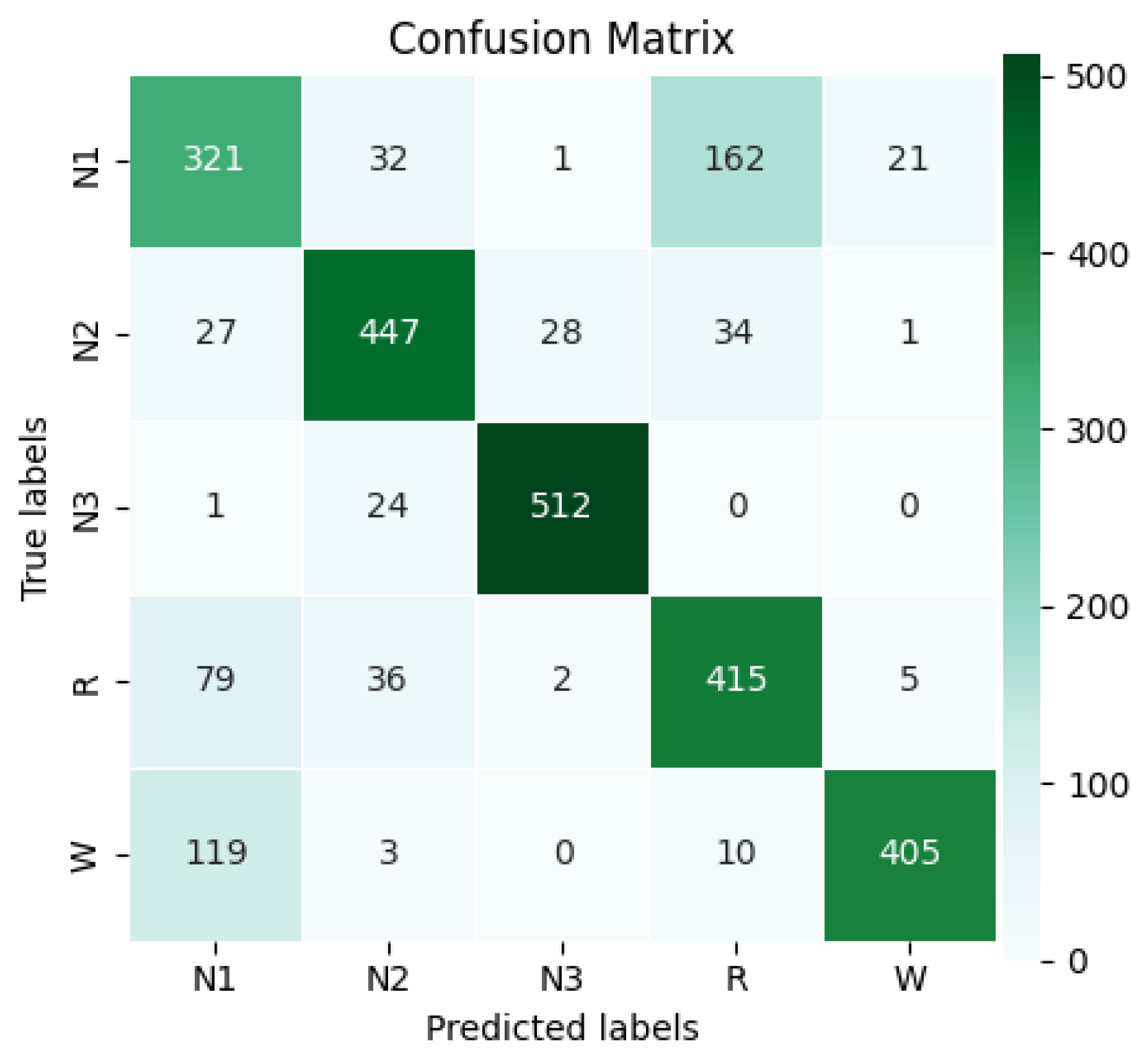
After each training iteration, the model evaluation on the validation data was performed by selecting the epoch where the validation loss reached its lowest point. The model was trained for up to 77 epochs, but early stopping with a patience value of 30 epochs was triggered at epoch 47, where the best loss was recorded. Due to the complexity of the network and the large EEG data, training required high-performance hardware and optimizations such as early stopping and batch tuning. The layer-wise computational cost analysis in the Methodology section highlights performance impacts, helping to identify bottlenecks and architectural optimization to ensure a balance of accuracy and efficiency. After completing the training session, the confusion matrix of the classification results was obtained, as shown in Figure 12.

This matrix represents 2685 predictions made by the model, corresponding to the processing of 8,055,000 samples, with 3000 samples per example and 537 examples per class. Class N1 had the fewest correct predictions, with a total of 321, representing the poorest performance. The accuracy for classes N2, R, and W was similar, achieving 447, 415, and 405 correct predictions, respectively. However, class N3 performed the best, with 512 correct predictions. The model achieved overall accuracy of 78.21%. Using the confusion matrix, the $TP$, $FP$, $TN$, and $FN$ were calculated for each class. The results of the calculation of the metrics per class, including the precision, recall, F1-score, specificity, NPV, and Jaccard index, are shown in

Table 3. Per-class validation performance metrics.

	Metric %
Class	Precision	Recall	F1-Score	Specificity	NPV	Jaccard
N1	58.68	59.78	59.23	89.48	89.90	42.07
N2	82.47	83.24	82.85	95.58	95.80	70.73
N3	94.29	95.34	94.81	98.56	98.83	90.14
R	66.83	77.28	71.68	90.41	94.09	55.85
W	93.75	75.42	83.59	98.74	94.14	71.81

. The classification results for each class are detailed below.

• N1: Class N1 was the most challenging for the model. The precision was 58.68% and recall was 59.78%, with an F1-score of 59.23%, indicating that the model correctly identified this class just over half the time, showing balanced but modest performance. The specificity was 89.48%, and the NPV was 89.90%, showing that the model is more reliable in rejecting this class than confirming it. The Jaccard index was 42.07%, reflecting weak agreement between the predictions and true labels.
• N2: Class N2 showed solid and balanced performance. The precision was 82.47% and recall was 83.24%, with an F1-score of 82.85%, reflecting good accuracy and detection and overall consistent results. The specificity was 95.58% and the NPV was 95.80%, showing effective distinction from other classes. The Jaccard index was 70.73%, indicating strong classification consistency.
• N3: Class N3 achieved the best overall performance. The precision was 94.29% and recall was 95.34%, with an F1-score of 94.81%, demonstrating excellent accuracy and sensitivity and outstanding balanced performance. The specificity was 98.56%, and the NPV was 98.83%. The Jaccard index was 90.14%, showing strong agreement between the predictions and actual values.
• R: For class R, the precision was 66.83% and the recall reached 77.28%, with an F1-score of 71.68%, indicating moderate precision with fairly good sensitivity and acceptable overall performance. The specificity was 90.41% and the NPV was 94.09%, reflecting the good detection of negatives. The Jaccard index was 55.85%, indicating moderate agreement between the predicted and true labels.
• W: Class W achieved 93.75% precision and 75.42% recall, with an F1-score of 83.59%, showing high precision and a good detection rate. The specificity was 98.74% and the NPV was 94.14%, demonstrating the model’s ability to avoid false positives. The Jaccard index was 71.81%, indicating good overall performance.

After computing the individual metrics per class, the macro-average for each metric was obtained. Additionally, Cohen’s kappa coefficient was calculated, resulting in a value of 0.7277, which indicates strong concordance between the predicted and actual class labels, with minimal influence of chance. The performance model metrics calculated in the validation step are presented in

Table 4. Classification results of the best model on the validation set.

Metric	Value
Overall Accuracy	78.21%
Precision	79.20%
Recall	78.21%
F1-Score	78.43%
Specificity	94.55%
NPV	94.55%
Jaccard	66.12%
Cohen’s Kappa	72.77%

.

Based on the previous results, the accuracy of 78.21% suggests that the system successfully classified most of the cases. The 79.20% precision indicates a strong ability to correctly predict positive cases, with a low false positive rate. The recall of 78.21% demonstrates the consistency of the model in detecting actual positive cases. The F1-score of 78.43% shows the harmony between precision and sensitivity. The high specificity and NPV, both at 94.55%, indicate strong performance in correctly identifying negative cases. Meanwhile, the Jaccard index of 66.12% suggests that the model can still improve in terms of achieving an exact match between the predictions and the class labels. Finally, the Cohen’s kappa value of 72.77% shows substantial alignment between the predicted outcomes and actual labels, largely excluding chance. These validation results show solid and consistent performance, suggesting that the model was effectively trained. They provide a reliable basis for the final evaluation.

4.7. Model Evaluation

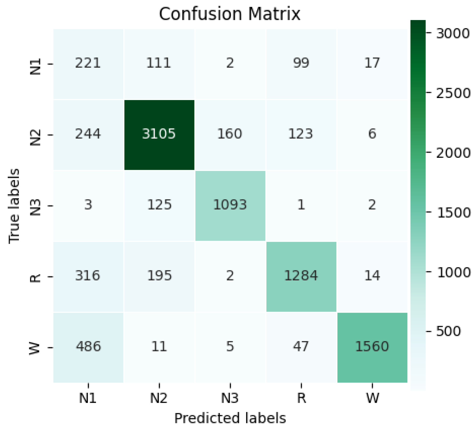
Once the best model was trained, its performance was evaluated in the test set. The confusion matrix shown in Figure 13 summarizes the classification results by class. Since this set was neither preprocessed nor balanced, the natural class distribution was maintained, allowing the model’s performance to be observed in a real-data context. In total, 9232 test examples were used, equivalent to 276,960 s of recordings (27,696,000 samples). The class distribution was as follows: N1 = 450, N2 = 3638, N3 = 1224, R = 1811, and W = 2109. This distribution is typical in sleep analysis, where N1 is often underrepresented and N2 is usually the most frequent stage, reflecting the natural prevalence of certain sleep cycle patterns.

According to the confusion matrix, the model correctly classified 221 N1 examples, 3105 N2, 1093 N3, 1284 R, and 1560 W. With these results, the overall accuracy of 78.67% was calculated for the test set, demonstrating the model’s ability to correctly classify most examples not used during training. Detailed class-wise metrics are shown in

Table 5. Per-class test performance metrics.

	Metric %
Class	Precision	Recall	F1-Score	Specificity	NPV	Jaccard
N1	17.40	49.11	25.70	88.06	97.12	14.74
N2	87.54	85.35	86.43	92.10	90.62	76.10
N3	86.61	89.30	87.93	97.89	98.36	78.46
R	82.63	70.90	76.32	96.36	93.14	61.70
W	97.56	73.97	84.14	99.45	92.81	72.63

. A summary of the performance metrics per class is presented below.

• N1: Class N1 remained the hardest to predict. The precision was 17.40% and recall 49.11%, with an F1-score of 25.70%, revealing limited performance in this class but with some success in detection. The specificity was 88.06% and the NPV 97.12%, indicating more reliable rejection than detection. The Jaccard index was 14.74%, reflecting poor overlap between the predictions and the true labels.
• N2: Class N2 maintained strong metrics. The precision was 87.54% and recall 85.35%, with an F1-score of 86.43%, indicating effective classification with balanced accuracy and coverage. The specificity was 92.10% and the NPV 90.62%, showing the reliable identification of non-N2 cases. The Jaccard index was 76.10%, confirming the consistent predictions.
• N3: Class N3 produced the most reliable results. The precision was 86.61% and recall 89.30%, with an F1-score of 87.93%, reflecting both accurate predictions and strong sensitivity. The specificity reached 97.89% and the NPV 98.36%, with a Jaccard index of 78.46%, showing a high degree of overlap with the true labels.
• R: For class R, the precision was 82.63% and recall 70.90%, with an F1-score of 76.32%, showing decent performance with slightly lower coverage. The specificity was 96.36% and the NPV 93.14%, indicating the effective rejection of incorrect cases. The Jaccard index was 61.70%, reflecting moderate agreement.
• W: Class W achieved 97.56% precision and 73.97% recall, with an F1-score of 84.14%, suggesting high accuracy and good but improvable detection. The specificity was 99.45% and the NPV 92.81%, highlighting an excellent ability to avoid false positives. The Jaccard index was 72.63%, supporting its solid overall performance.

These results reveal varying performance across different classes, with N1 being the most difficult to classify and N3 performing the best. The poor performance of N1 in several metrics can be attributed to its underrepresentation in the data, a common challenge in unbalanced classification problems. In contrast, classes N2, N3, R, and W showed consistent and balanced performance. These differences underscore the importance of addressing class imbalance to improve the accuracy and balance in predictions. After calculating the metrics for each class, macro-average metrics were derived, and Cohen’s kappa coefficient was calculated for the test set matrix, yielding a value of 73.39%, confirming the model’s consistency and the validity of its predictions. The results of the overall test metrics are presented in

Table 6. Classification results of the best model on the test set.

Metric	Value
Overall Accuracy	78.67%
Precision	74.35%
Recall	73.73%
F1-Score	72.10%
Specificity	94.77%
NPV	94.41%
Jaccard	60.73%
Cohen’s Kappa	73.39%

. In the following, a comparative analysis between the test results and validation results is provided.

• Overall accuracy: The accuracy on the test set was 78.67%, indicating relatively accurate classification in general. This result is satisfactory, especially given the significant class imbalance in this multiclass classification problem. The close match with the accuracy of 78.21% in the validation set suggests good consistency between model training and generalization to new data.
• Precision: The precision of 74.35% indicates an acceptable rate of correct predictions for the positive class. However, compared to the precision of 79.20% on the validation set, it can be inferred that the underrepresentation of class N1 limited the performance in the test set.
• Recall: The recall of 73.73% indicates that the model successfully classified most of the positive samples. This is consistent with the recall of 78.21% from the validation set, indicating that the model’s capacity to identify positive classes showed minimal variation between the two sets.
• F1-Score: The F1-score of 72.10% indicates a reasonable equilibrium between the precision and recall metrics. The drop in the F1-score from the validation set, where it was 78.43%, is mainly due to the significant decrease in precision for class N1 in the test set.
• Specificity: The specificity of 94.77% suggests excellent performance in identifying negative samples, consistent with the specificity of 94.55% from the validation set, reflecting a low false negative rate.
• NPV: The NPV of 94.41% indicates the effectiveness of the model in accurately identifying negative classes, corroborated by the NPV of 94.55% observed in the validation set.
• Jaccard Index: The Jaccard index of 60.73% indicates acceptable similarity between the model outputs and the actual labels, although there is room for improvement compared to the Jaccard index on the validation set of 66.12%. The difference is mainly due to the class imbalance for N1.
• Cohen’s Kappa: Finally, the Cohen’s Kappa score of 73.39% indicates a high degree of consistency between the predictions and the true labels, which implies that the model’s decisions are not coincidental. This value, slightly higher than the 72.77% from the validation set, suggests consistent performance in generating reliable agreements.

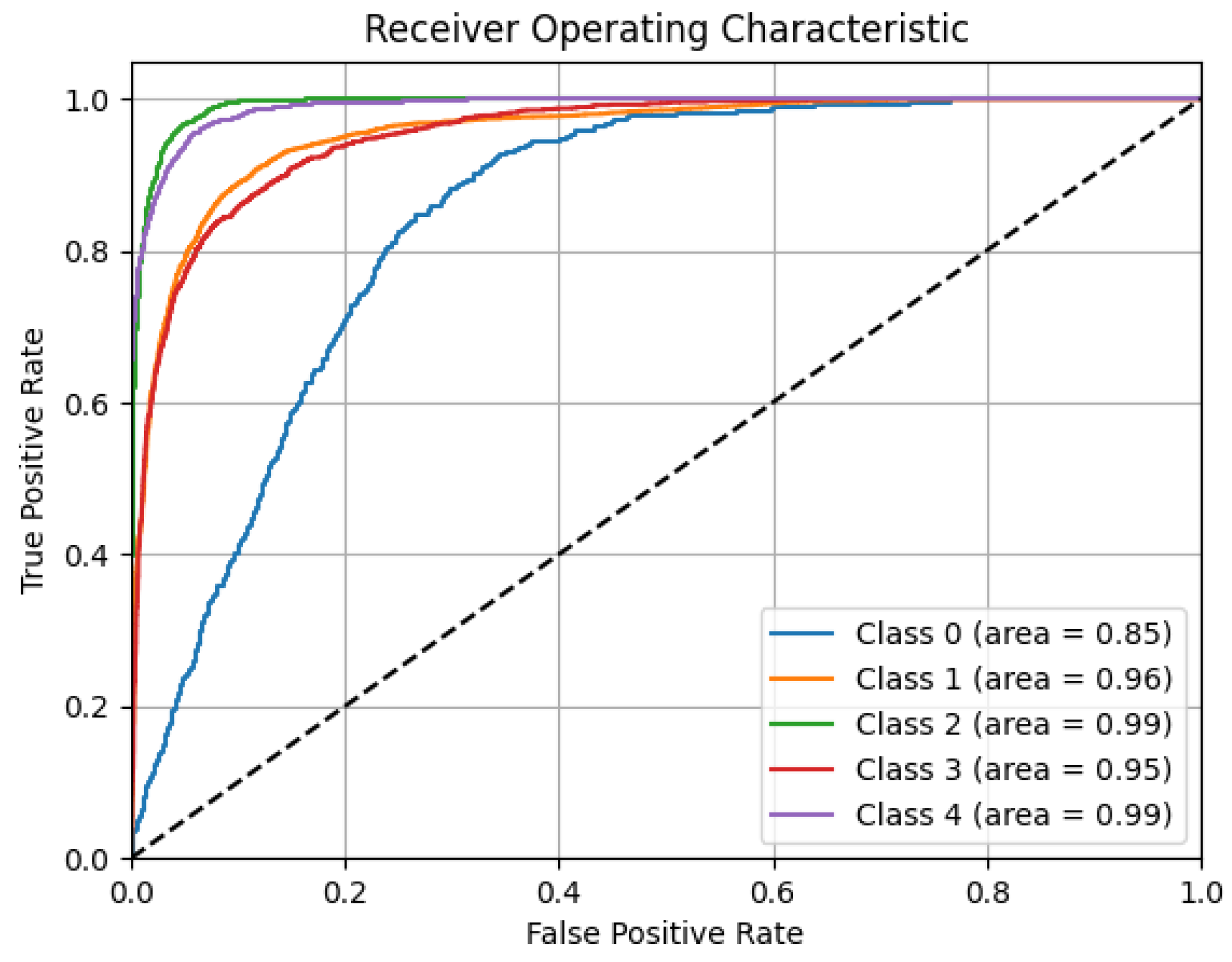
The results show the model’s overall strong performance, effectively managing class imbalances and excelling in identifying negative classes. Although there is room for improvement in classifying less frequent categories, the model maintains a good balance between precision and recall, minimizes random predictions, and generalizes well across datasets. To reinforce these outcomes, Figure 14 presents the overall ROC curve of the model, which reflects the model’s ability to differentiate among classes using different decision thresholds.

The area under curve (AUC) values reflect high performance for nearly all classes: W and N3 both achieve an outstanding AUC of 0.99, while R and N2 also produce excellent results, with AUCs of 0.95 and 0.96, respectively. Although the N1 class has a lower AUC of 0.85, it still indicates an acceptable discriminative ability, especially considering its low representation in the data distribution. The ROC curves illustrate the model’s strong ability to distinguish between sleep stages, maintaining high true positive rates while minimizing false positives, even with unbalanced class distributions.

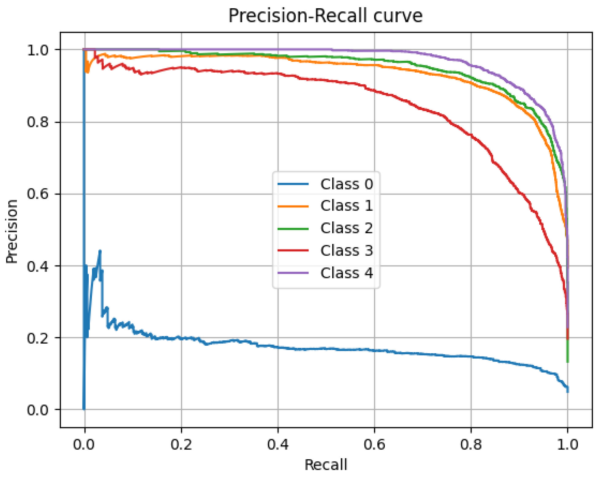
Complementarily, the model’s overall precision–recall curve, particularly valuable in evaluating performance under class imbalances, is presented in Figure 15. The curves for classes 1 through 4 (N2, N3, R, and W) remain high, indicating a favorable equilibrium between recall and the correctness of positive predictions. In particular, N3 and W exhibit the most stable and elevated curves, maintaining high precision levels even with increasing recall. In contrast, the precision of class N1 decreases as the recall increases, reflecting the difficulty of the model in identifying this class without generating false positives. Although the model exhibits strong results across most stages, improvements are still needed to handle less frequent categories.

The per-class metrics and the analyses conducted confirm the model’s classification capabilities across various sleep stages, despite variations due to class imbalance. Although N1 performs poorly relative to more prevalent stages, such as N2 and N3, the model manages the dominant classes well, with a good balance between precision and recall. Global metrics such as the F1-score and Jaccard index indicate its solid classification capacity, which could be further improved by addressing the dataset imbalance. The ROC and precision–recall curves reinforce the evidence of the model’s reliable discriminative power. Despite its limitations with minority classes, the model demonstrates strong generalization and overall robustness. The next section will provide a detailed discussion of these results, their implications, and comparisons with previous studies to guide future model development.

4.8. Discussion

When the process moves from validation to testing, the model still filters out negative examples reliably, showing that its nonstage rule holds up in real data. There is a small but expected drop in capturing true positives for the rare stages when faced with the natural imbalance of the test set; this does not negate our results but points to areas for fine-tuning (for example, through rebalancing or class-aware loss). The overall agreement remains similar, meaning that most errors happen in the least common classes, while the major stages remain solidly identified. These findings show that the model is generally robust and suggest simple steps to strengthen its ability to identify underrepresented patterns without degrading its strong performance on the more frequent ones.

To validate the effectiveness of the proposed model, we compare its accuracy with that of leading sleep stage classifiers (

Table 7. Comparison with state-of-the-art approaches.

Work	Database	Approach	Overall Accuracy (%)
[25]	Toranomon	K-Means	75
[24]	Sleep-EDFx	LGBM, XGBoost	77
[26]	-	SOM, SVM	70.43
[23]	Sleep-EDF	CFC, LDA	75
[5]	Sleep-EDF Expanded	CNN	74
[28]	ISRUC-Sleep	CNN, BiLSTM	84.1
[29]	Sleep-EDF 13, Sleep-EDF 18	CNN, BiLSTM	84.26
[30]	Sleep-EDF 20, Sleep-EDF 78	CNN, BiLSTM	91.44
This work	Sleep-EDF Expanded	CNN, BiLSTM	78.67

). The traditional methods—K-Means (75%) [25], SVM (70.4%) [26], CFC + LDA (75%) [23], and LGBM + XGBoost (77%) [24]—achieve reasonable results but lack the ability to capture subtle time-dependent features (e.g., sleep spindles, K-complexes). They also rely on manual feature extraction, which demands expert knowledge, limits scalability, and hinders practical deployment. Deep learning models extract features directly from raw data, streamlining processing and improving the scalability and generalization to large datasets. In Sleep-EDF Expanded, pure CNNs achieve 74% accuracy [5]. CNN-BiLSTM models improve the performance, reaching 84.1% on ISRUC-Sleep [28] and 84.26% on Sleep-EDF 13 and 18 [29], all using single-channel EEGs. Meanwhile, a multichannel approach on Sleep-EDF 20 and 78 achieves 91.44% accuracy [30]. Hybrid models combining CNNs and LSTM achieved the best performance in capturing EEG dynamics. However, based on the computational cost formulas outlined in the Methodology section, pure CNNs may be significantly more efficient, as their structure favors parallel processing. This highlights the importance of weighing accuracy against resource demands in real-world applications.

The proposed CNN–BiLSTM–Attention model achieves an overall accuracy rate of 78.67%, slightly below the top-performing models [28,29,30]. However, our approach includes methodological elements that aim to improve the generalization and control bias. In particular, we introduce E-LRUS, which subsamples entire 30 s segments to preserve temporal coherence, unlike conventional oversampling or synthetic methods. This enabled the class N3, which was the second most underrepresented after N1, to achieve the highest performance (precision: 86.61%, recall: 89.30%, F1-score: 87.93%), outperforming more frequent classes like N2 and W. E-LRUS thus facilitates the robust detection of underrepresented classes without skewing toward dominant ones. In contrast, several state-of-the-art studies lack explicit balancing or preprocessing, possibly leading to bias or overfitting despite their higher accuracy.

The method demonstrates solid performance in most sleep stages, with N1 remaining the most challenging to classify. The model effectively distinguishes N1 from N3 due to clear spectral and temporal differences. However, it shows moderate difficulty in separating N1 from N2 during validation and more substantial confusion with W and R, particularly in the test set. These errors likely result from overlapping transient EEG patterns and the inherently variable and transitional nature of N1. Despite class balancing, its low intraclass consistency and the absence of distinct biomarkers continue to limit the classification performance. Further improvements could involve adapting the complexity of the model by adjusting the depth of the network or exploring alternative architectures and training schemes. Repeating E-LRUS sampling with varied random seeds and merging datasets could also increase N1’s representation without adding artificial variability, although care is needed to avoid memorization. Enhancing the N1 classification in these ways would significantly improve the model’s generalizability and clinical applicability.

5. Conclusions

The proposed hybrid architecture, which combines CNNs, BiLSTM layers, and attention mechanisms, demonstrated solid performance by extracting meaningful features from raw EEG data. It achieved overall accuracy of 78.67% and an F1-score of 72.10%, reflecting balanced performance across sleep stages. To improve its generalization and reduce bias, the model incorporates the E-LRUS procedure, which subsamples entire 30 s segments to preserve temporal coherence. This strategy contributed to strong performance in N3, the second most underrepresented stage, with an F1-score of 87.93%, outperforming more frequent stages such as N2 and W. By balancing the training data without altering its natural structure, the model mitigated overfitting and enabled robust detection between stages. This synergy between the architecture and data handling supports a reproducible end-to-end solution for biomedical signal classification.

Future work should address class imbalance through targeted data augmentation and class-aware training, while also integrating time- and frequency-domain processing within deeper or residual network architectures to capture more intricate patterns with fewer parameters. Additional improvements may include refined architectures, multiscale temporal features, temporal context enhancement, and specialized loss functions designed to better detect the underrepresented stage N1. Since model performance depends on factors such as the dataset size, diversity, class imbalance, and design choices, continued efforts could focus on hybrid architectures, advanced data enhancement, and balanced training strategies to improve the reliability, generalizability, and clinical applicability. Incorporating complementary modalities such as EMG or EOG, developing interpretability tools for clinicians, and exploring lightweight model variants suitable for portable devices will further support real-world clinical adoption. Extending this framework to other EEG-based diagnostic tasks could broaden its impact in sleep medicine.