Article

Asymmetric Magnetohydrodynamic Propulsion for Oil–Water Core Annular Flow Through Elbow

1
School of Mechanical and Power Engineering, Zhengzhou University, Zhengzhou 450001, China
2
School of Chemistry, Zhengzhou University, Zhengzhou 450001, China
3
School of Physics and Engineering, Zhengzhou University, Zhengzhou 450001, China
4
School of Science, Henan Agricultural University, Zhengzhou 450002, China
*
Authors to whom correspondence should be addressed.
Appl. Sci. 2025, 15(12), 6828; https://doi.org/10.3390/app15126828
Submission received: 28 February 2025 / Revised: 10 June 2025 / Accepted: 11 June 2025 / Published: 17 June 2025

Abstract

:
The use of oil–water rings has become an emerging, effective, and energy-saving method of transporting heavy oil. Maintaining the shape of the oil–water ring and preventing rupture during the transport of heavy oil are of great scientific significance in oil–water annular flow transportation. To ensure the oil–water ring passes smoothly through the elbow without rupture, this article proposes an asymmetrical magnetohydrodynamic (MHD) propulsion method to utilize the significant difference between the conductivity of heavy oil and electrolyte solution to achieve an accelerating effect on the outer water ring. The magnetohydrodynamic device designed by this method can generate a magnetic field and provide Lorentzian magnetic force to achieve the asymmetric acceleration of the oil and water rings, to homogenize the water ring velocity on the inner and outer elbows, to push the deviated oil core back to the center of the pipeline, and to repair the rupture of the water film. The flow state of the oil–water ring in the bend pipe under the joint action of the electric field and magnetic field is simulated by a differential MHD thick oil simulation flow model, which confirms that the device can realize the repair of the oil–water ring flow at the bend pipe and ensure that the oil–water ring flow passes through the bend pipe stably. Meanwhile, the effects of coil current, electrode plate voltage, and the conductivity of electrolyte solution on the morphology and velocity of the oil–water ring in the elbow are investigated. In addition, the role of the device in maintaining the morphology under different gravitational conditions is investigated. These results provide a reference design for related devices and offer a new approach to heavy oil transportation.

1. Introduction

With the depletion of the world’s light and medium oil reserves, heavy oil is becoming a strategic alternative resource that countries worldwide are scrambling to study. The characteristics of heavy oil such as high viscosity, high density, and poor fluidity bring great difficulties and challenges to exploitation, storage, and transportation. Currently, the pipeline transportation of heavy oil is mainly achieved through heating [1,2], emulsification [3], doping diluent [4,5], and other methods. However, these methods have limitations and drawbacks; for example, the heating method has the disadvantages of high energy consumption and the expensive cost of pipeline construction. For this reason, an oil–water annular transportation method [6,7,8] has been developed, which can significantly reduce the energy consumption of transportation, enable room-temperature transportation, and become a potential method of heavy oil transportation.
Oil–water annular flow conveying involves the utilization of an annular flow pattern formed by two immiscible fluids with significantly different viscosities in a horizontal pipe, commonly referred to as “core annular flow”. In this configuration, the oil phase tends to occupy the central region of the pipe due to the viscosity contrast, while the lubricating fluid (typically water) forms a surrounding annular layer along the pipe’s inner wall [8]. In the past few years, research on oil–water annular flow has mainly focused on the design optimization of the water ring generator [9,10], the analysis of oil–water two–phase flow characteristics and the pressure drop law [11,12,13,14,15,16], and the method of enhancing the stability of oil–water annular flow [17,18,19,20,21,22,23]. The stability of oil–water annular flow has a decisive impact on the practical application of water-lubricated oil transportation. Researchers have explored the transport stability of oil–water rings from many aspects, including the influencing factors of oil–water annular flow in various types of pipelines (horizontal, vertical, and curved) [24,25,26,27,28,29,30]. Most researchers have explored the above aspects through experiments. Franchi et al. [13] experimentally explored the role of the experimental determination of flow patterns, pressure gradients, and phase holdup during the two-phase flow of a very viscous oil–water mixture in a downward inclined pipe configuration. Housz et al. [16] set up an experiment to experimentally and numerically study the annular flow of oil and water cores in a horizontal pipe, focusing on the effects of the presence of turbulence in the water annulus on the oil–water annulus flow. Cavicchio et al. [18] conducted a thick oil–water vertical upward flow experiment to investigate the effects of viscosity on core annular flow parameters. Sun et al. [22] set up an experimental bench and conducted an experimental program using a model oil (201 methyl silicone oil) and independently prepared aqueous foams to investigate the flow pattern and resistance characteristics of thick oil in plumbing under the action of aqueous foams to verify the effectiveness of thick oil in reducing resistance in production wells. Yang et al. [26] investigated flow pattern transitions and concentration distribution during the simultaneous pipe flow of oil–water two-phase flow through the horizontal and vertical sections through a series of experiments. Paul et al. [31] investigated the pressure drop and flow pattern of oil–water flows in a 19 mm ID clear polyvinyl chloride pipe consisting of a U-bend with a radius of curvature of 100 mm, and the associated pressure drop laws were obtained by varying the velocity of the oil–water phase in the pipe through a series of experiments. Some researchers have also conducted related studies through simulations. Shi et al. [14] examined the capability of a VOF model to simulate horizontal oil–water two-phase flow with matched density and a medium viscosity ratio under flow rates corresponding to different flow patterns, namely, core annular flow, oil plugs in water, oil bubbles in water, and dispersed flow. Jiang et al. [25] used CFD simulations to find the hydrodynamic conditions under which the flow in the core annulus becomes unstable and the oil wave comes into contact with the pipe wall, and they obtained a series of relevant conclusions. Liu et al. [30] used simulation to develop a quasi-three-dimensional numerical model of the axial pressure gradient, interface height, water content, and flow field in an oil–water two-phase stratified pipe flow, which solves the governing equations of steady axial momentum and mass conservation equations and solves a low-Reynolds-number k~ε turbulence model of vortex viscosity in a bipolar coordinate system, which facilitates the description of the curved interfaces and the mapping of the physical domain. Wu et al. [32] used the computational fluid dynamic (CFD) method to study and analyze the effects of the inlet water fraction, the oil–water property, and geometric parameters on hydrodynamic performance in the development of core annular flow (CAF), and the results could provide a reference for the design of 90° elbow structures and the optimization of flow parameters. Jiang et al. [33] used numerical simulation to compare the interface fluctuations and energy-saving performance of oil–water annular flow under different pipeline structures, flow parameters, and fluid properties, which provide a reference for the design of heavy oil transportation pipelines, the analysis of interface fluctuation, and the energy-saving evaluation of oil–water annular flow. The CFD simulation was also used by Gupta et al. [34] to study the axisymmetric, laminar–laminar oil–water core annular flow in a pipe (radius 14.2 mm) without the gravitational effect under three different channel conditions: vertically upward flow, vertically downward flow, and without considering the gravitational effect.
Although the above studies apply numerical simulation methods to study the influence of parameters (such as density, viscosity, and others) in oil–water characteristics on the stability of oil–water annulus flow in pipelines and provide references for the design of pipes and the optimization of oil–water flow parameters in actual production, some limitations still exist. The range requirements of oil–water characteristics, transport parameters, and other related parameters make oil–water annular flow transport have certain restrictions. For elbows where the rupture of the oil–water ring is more serious, the oil–water parameters and design of the elbows need to be set more accurately to ensure the oil–water ring passes through stably, which significantly limits the development and practical application of oil–water annular flow.
To ensure the smooth passage of the oil–water ring through the elbow without the restriction of pipe flow parameters, a universal and independent method urgently needs to be developed to stabilize the oil–water ring annular flow in elbows.
Here, we present an asymmetrical magnetohydrodynamic (MHD) propulsion method to utilize the significant difference between the conductivity of heavy oil and an electrolyte solution to achieve the accelerating driving effect on the outer water ring. Without changing the design of the pipeline, the device can break through the range requirements of oil–water properties and oil–water ring conveying parameters by changing the voltage, current, or water ring conductivity and achieve the perfect conveying of the oil–water ring. The flow state of the oil–water ring in the elbow under the combined action of the electric and magnetic fields is simulated by using the differential MHD heavy oil flow model, and the Lorentzian magnetic force provided by the MHD field achieves the asymmetric acceleration of the oil–water rings to homogenize the water ring velocity on the inside and outside of the elbows and pushes the deviated oil cores back to the center of the pipeline to repair the water film breakage. Meanwhile, numerical simulations were performed to investigate the effects of coil current, electrode plate voltage, the conductivity of electrolyte solution, and gravity directions on the morphology and stability of the oil–water annular flow in an elbow under asymmetric MHD propulsion.

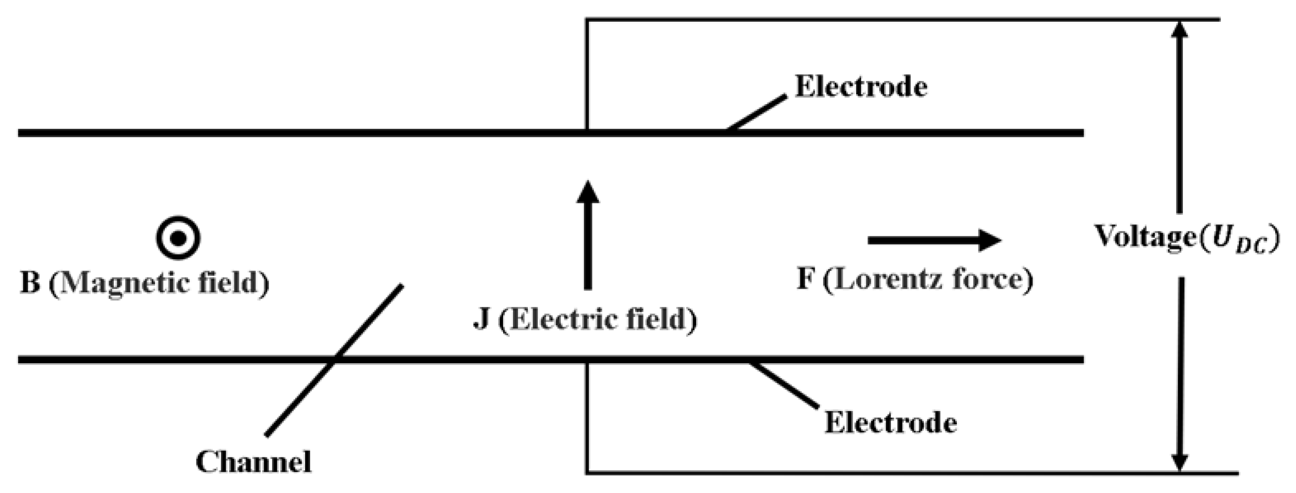
2. Magnetohydrodynamic Principles

Magnetohydrodynamics (MHD) is the study of electrically conducting fluids, and the conductive medium is usually plasma or liquid metal, in which the magnetic field plays a dynamical role [35]. At present, the main research fields of MHD are astrophysics [36,37,38], micro- and nano-robot drive [39,40,41,42,43], accelerators [44,45,46,47,48], and so on [49,50,51]. Magnetohydrodynamics is based on the basic principle that through the interaction between the magnetic field generated by the electromagnetic coil and the electric field generated between the electrode plates, charged particles are subjected to the Lorentz force in the space between the electric and magnetic fields, resulting in definite acceleration [52,53,54]. The specific operating principle is shown in Figure 1. As can be seen from the diagram, the charged particle is accelerated in the direction of the force by the Lorentz force generated by the interaction of an applied static magnetic field with a constant voltage. Therefore, the principles of MHD can be used to accelerate or decelerate the electrolyte solution and to change the direction of fluid flow [55]. Depending on the type of electrical current applied, magnetic fluids are subdivided into DC (Direct Current) and AC (Alternating Current) magneto-fluid accelerators [56,57,58]. As heavy oil is constantly moving in the pipeline, and the AC–type magneto-fluid accelerator is unsuitable for scenarios where the conductor is continuously moving, the DC–type magneto–fluid accelerator was chosen for this design.
In the process of oil and water two-phase flow through the elbow, due to the centrifugal force at the bend, gravity, and other factors, the center of the pipeline oil phase will have an impact on the water phase of the package, resulting in the rupture of the oil–water ring. The oil–water circulation conveying process is realized by the water ring wrapping the oil ring. When the oil–water ring flows through the elbow, due to centrifugal force, oil–water density difference, and other factors, the outer water ring is thrown to the outside of the pipe, and the thickness of the water ring becomes insufficient to support the oil ring, which destroys the original annular structure, thus leading to the rupture phenomenon. After the rupture of the oil–water annulus, the oil phase wrapped in the annulus due to the density difference will naturally float and may come into contact with the pipe wall to affect the movement of the outer water ring, accelerating the separation of the oil–water phase stratified flow. At the same time, the high viscosity of heavy oil will cause it to adhere to the pipe wall and form scaling, which will block the pipeline over time and cause a series of effects on heavy oil transportation. The differential MHD heavy oil flow stabilization accelerator in this design relies on the DC–type magneto-fluid accelerator design principle. By adding a set of electromagnetic devices at the elbow, the differential drive of the oil and water phases is achieved, so the oil–water ring can maintain a stable oil–water annular flow pattern through the elbow pipe section. When the oil–water ring passes through the elbow, the device outside the pipe will provide external force to the flowing water phase to ensure that the water phase will not break. The device will also act on the oil phase to prevent the oil phase from floating upwards, realizing the repair of the soon-to-be-damaged oil–water ring and ensuring that the oil–water ring passes through the transportation process smoothly in the elbow.

3. Simulation Establishment

This article focuses on the simulation and analysis of the established differential MHD heavy oil stabilization accelerator model using simulation and analysis software such as COMSOL Multiphysics® 6.1 [59] and SOLIDWORKS(R) Premium 2021 SP0.0.

3.1. Model Design

The oil–water ring flowing through the elbow is ruptured by centrifugal force, so the structural design of the elbow is critical. In this article, the “L” elbow is modeled as shown in Figure 2a, and its dimensions are specified in Table 1. Meanwhile, the flow direction of the oil–water ring in the pipeline and the direction of gravity are shown in Figure 2a. The differential MHD heavy oil flow stabilization accelerator relies on a magnetic fluid acceleration device to ensure the stable transport of thick oil at the elbow. In the conventional magnetohydrodynamic acceleration device, the magnetic guide sleeve, the electrode plate, and the electromagnetic coil are set coaxially with the pipe. Since the electromagnetic field generated by the densely mounted waves will intervene excessively in the heavy oil transportation process, four electromagnetic coils and two pairs of electrode plates are selected for the final design solution, as shown in Figure 2b. In addition, four solenoid coils and two pairs of pole plates are set coaxially with the pipe and hide the breathable sleeve, but they are simplified in Figure 2b in consideration of the fact that a few parts do not work during the simulation. The specific dimensions of the components shown in Figure 2b are shown in Table 2. In addition, two pairs of electrode plates and four solenoid coils are set coaxially with the pipeline with a hidden breathable sleeve.
According to the design model data above, the model is drawn in the relevant simulation software, as shown in Figure 2c,d. The position of the device components and the heavy oil transportation pipeline are indicated in the figure. To accomplish the accelerating effect on the water ring on the outside of the pipe shown in Figure 2c, in the following simulation process, the coils B-D, shown in Figure 2b,d, are energized, 220 V is applied to the positive pole plates, and 0 V is attached to the negative pole plates. As can be seen in Figure 2c, the oil–water ring transported in the pipeline consists mainly of red-colored heavy oil and blue-colored electrolyte solution. During the simulation, the flow direction and gravity direction of the oil–water ring in the pipe is consistent with the orientation in Figure 2a.

3.2. Related Parameter Settings

The created model is imported into the simulation software, and the specific parameters of the simulation are set as follows:
  • Parameter setting of heavy oil and electrolyte (water) solution: Oil core length 60 mm, dynamic viscosity 0.2 Pa·s, density 960 kg∙m−3, input initial velocity 0.1 m∙s−1; dynamic viscosity of electrolyte (water) solution 0.001 Pa·s, conductivity 5 m·s−1, density 1000 kg∙m−3, relative dielectric constant 81, input initial velocity 0.05 m·s−1.
  • Selection of pipe: The pipe wall conditions are chosen as no slip, the direction of gravity is along the negative path of the Y-axis, the reference pressure level is 1 atm, the temperature is 293.15 K, and the acceleration of gravity is g.
  • Magnetic field parameter setting: The magnetic field action range consists of all domains including air, and the relative permeability and electrical conductivity of relevant materials are selected in COMSOL Multiphysics® [59] software’ material library. Coil excitation is current, the current is set to 8 A, the number of coil turns is 100, and the coil wire conductivity is 6 × 10 7 S·m−1.
  • Electric field parameter setting: The electric field acts on four electrode plates as well as the water and oil phases, the voltage is set to 220 V, and the same parameter is set relative to two electrode plates, one pair of which is 220 V and the other pair of which is set to 0 V, which constitutes the positive and negative poles to provide current for the fluid.
  • Condition setting at the entrance and exit of the pipe: The boundary conditions at both the entrances and exits are set to fully developed flow, the average air pressure at the outlets is 0 kPa, and the hydrostatic pressure compensation is turned on.

4. Discussion

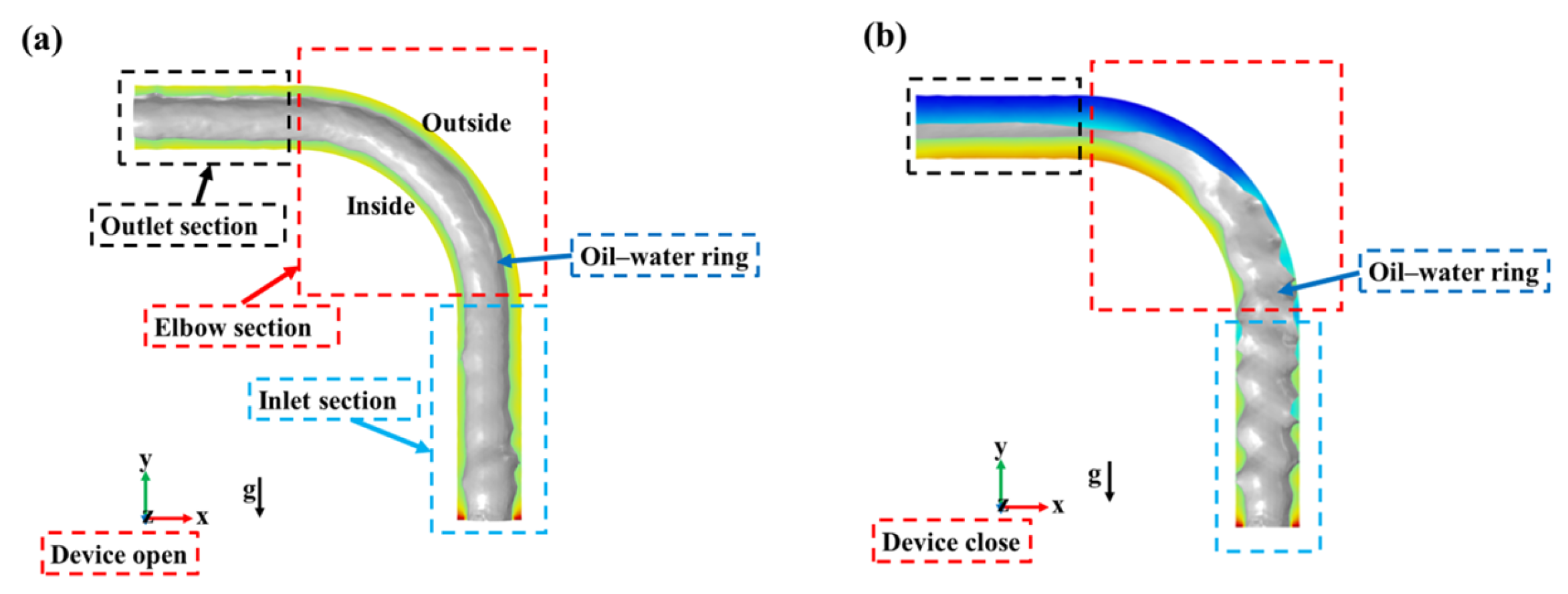
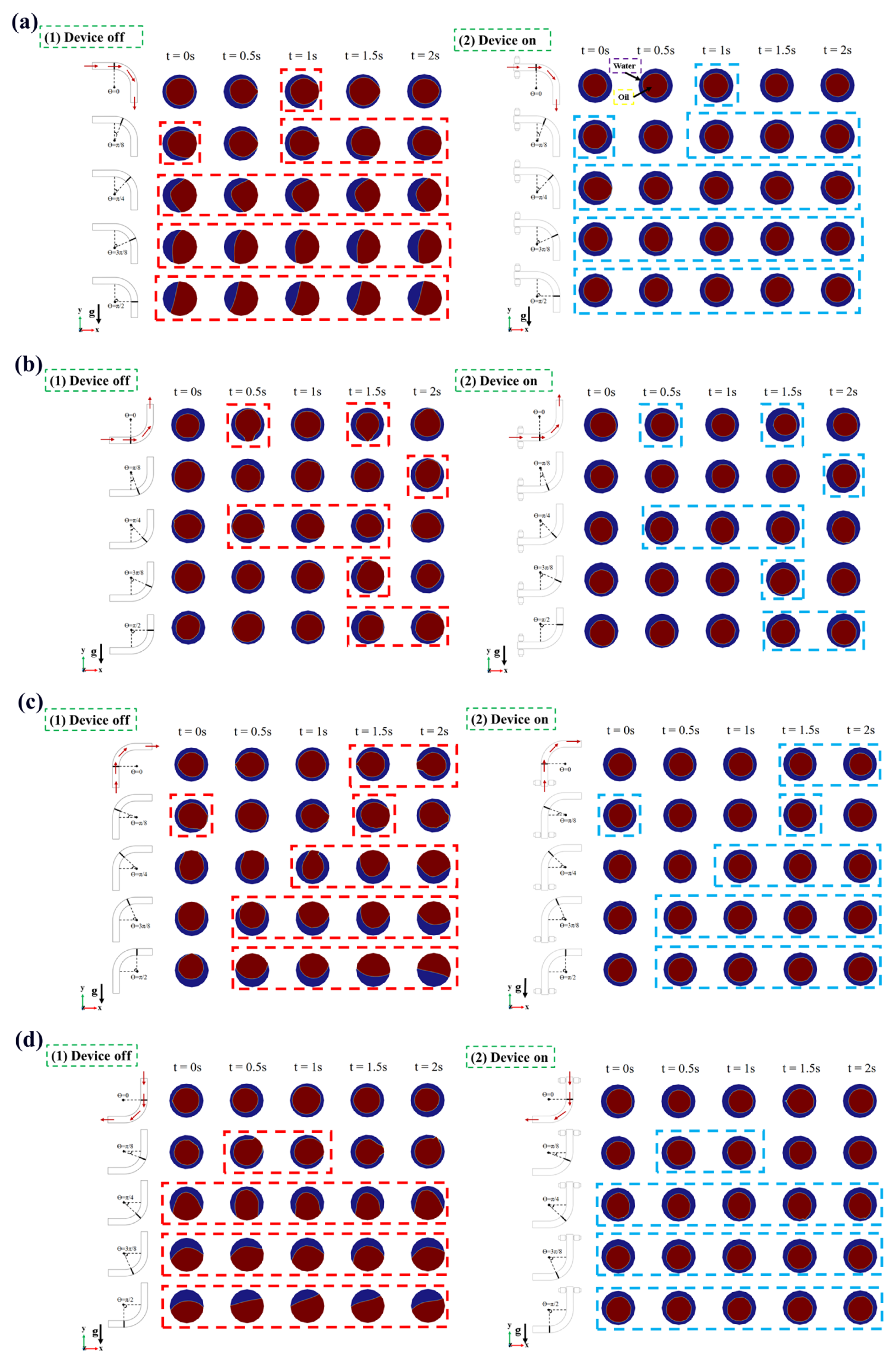
4.1. Oil–Water Interface Evolution

After the above parameters are set, the simulation of the oil–water loop flowability in the elbow is carried out, and the specific evolution is displayed in Figure 3.
Figure 3a shows that the conveying pipeline is divided into three sections for study, namely the inlet section (blue frame), the elbow section (red frame), and the outlet section (black frame). The oil phase always remains at the center of the pipe after a short period of flow development after the device is turned on, the flow pattern of which fluctuates slightly is generally more stable, and the water phase wraps around the outside of the oil phase to move forward through these three sections. However, when the differential MHD heavy oil flow stabilization accelerator is turned off, with the fundamental conditions like pipe flow conditions and oil–water initial velocity settings unchanged, the oil–water ring shape of the inlet section fluctuates widely, the oil–water ring shape of the elbow section breaks extensively, and the oil–water ring at the outlet is in a mixed state, as shown in Figure 3b. Due to the centrifugal force at the elbow, the oil phase will squeeze the water phase on the outside of the pipe when it passes through the elbow pipe, while the thickness of the water ring is not sufficient enough to isolate the oil phase from the pipe wall, resulting in the oil phase coming into contact with the pipe wall. During the subsequent transportation process, the oil and water phases will separate and stratify the flow due to other factors like gravity, resulting in the loss of the function of oil–water ring transport. By comparing the morphology of the three parts of the oil–water rings in Figure 3a,b, the device can achieve the asymmetric acceleration of the water ring by using the magnetic fluid principle for the oil–water rings in the elbow to ensure that the oil–water rings pass through the elbow section of the pipeline smoothly.

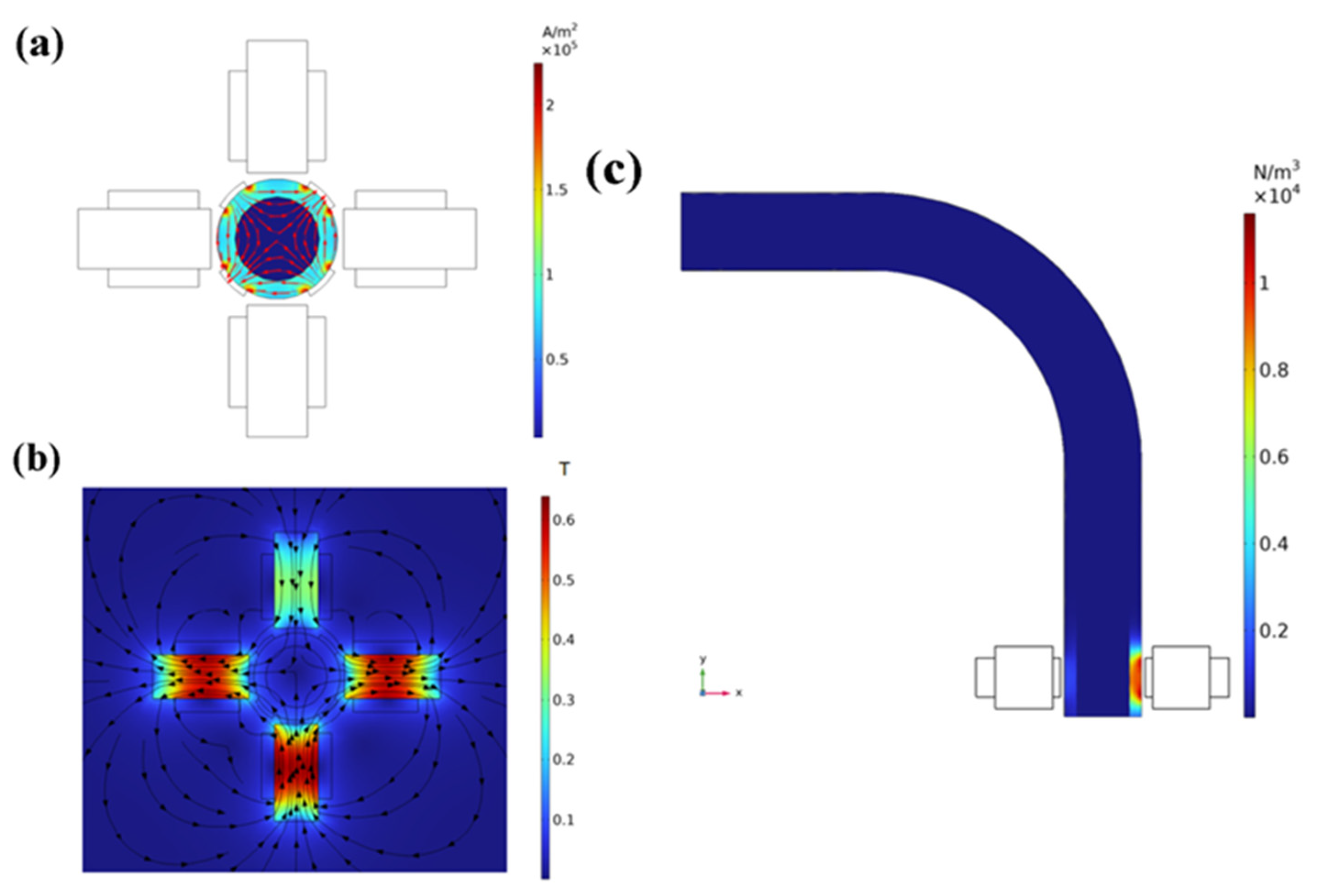
4.2. Electromagnetic Field

Electromagnetic field analysis focuses on the simulation analysis of the acceleration model in the differential MHD heavy oil flow stabilization accelerator model, including the simulation analysis of the magnetic field provided by the electromagnetic coil, the analysis of the electric field provided by the electrode plate, and the analysis of the Lorentz force supplied by electromagnetic field coupling.
After adjusting the direction of the current in the electromagnetic coil according to the desired direction of the Lorentz force and the positive and negative poles of the electrode plate, the influence of the electric and magnetic fields and the Lorentz force on the magnetohydrodynamic accelerator is analyzed. According to the definition of magnetic flux density, the magnitude of the magnetic field strength “B” can be expressed in terms of the magnetic flux density mode, and the magnetic flux density is used in this paper to indicate the strength of the magnetic field.
Figure 4a reflects a cloud of current density distribution within the pipe. Due to the high conductivity of the electrolyte liquid used in this simulation, a certain amount of current is generated in the electrolyte solution used in the pipe when a specific voltage is applied to its outside. Compared to electrolyte fluids, the conductivity of the heavy oil transported in the pipeline is minimal, and no electrical flow is generated when an external voltage is applied. Consequently, the magnitude of the electrical flows in the oil phase will not be calculated in this simulation, and this is the reason why only the electrolyte solution is given a differential drive during this simulation.
In Figure 4b, the distribution of the magnetic field, the direction of the magnetic flux lines, and the flux density produced by the electromagnetic coil can be seen. Magnetic flux density is used as the primary way to measure the strength of a magnetic field, and the different shades of colors in the graph represent the difference in magnetic flux density [60]. The magnetic flux density at the uppermost coil with the current set to 0 A is significantly lower than that of the other three coils with 8 A current settings. Moreover, the distribution of the Lorentzian magnetic force generated under the action of the magnetic and electric fields is reflected in Figure 4c. Since the magnitude of Lorentz force is determined by the magnetic field strength and current density, the differential pushing effect on the oil–water ring can be achieved by adjusting the electrode plate voltage and the coil winding current parameters to change the magnitude of Lorentz force.

4.3. Flow Field

Differential MHD heavy oil flow stabilization accelerator model flow field analysis is based on the electromagnetic field simulation analysis, still using COMSOL Multiphysics® [30] software for the calculation and analysis of the coupling between the electromagnetic field and the flow field, including the flow pattern of the oil–water annular flow in the elbow, the flow velocity distribution, and other content.
Research on the fluid velocity inside the pipe is of great significance for the practical application of the device, so this paper uses two methods, particle tracking and probe analysis, based on the simulation analysis to better study the flow process of the oil–water ring inside the pipe.
First of all, the analysis of the fluid velocity cloud inside the pipe is shown in Figure 5. Since the initial velocity of the oil phase is higher than that of the water phase, the red portion in the center of the pipe (oil phase) has a greater velocity than the blue portion at the edge of the pipe (water phase). Figure 5a shows that when the device is opened, there is a significant change in the velocity of the oil–water ring in the pipe by the electromagnetic force (Lorentz forces) provided by the device, with a higher amount of change in the speed on the side affected by the electromagnetic forces. Meanwhile, the A-A’ section at the acceleration region (region of device action) in Figure 5a shows that the device accelerates the outer water ring. The B-B’ section shows the red area (oil phase) distributed in the central region of the pipeline and the blue area (water phase) wrapped around the red area, neither of which breaks through the border of the oil–water ring. The velocity cloud of the pipeline when the device is not turned on is shown in Figure 5b. From the left side of the pipeline velocity cloud, the red area (oil phase) and blue area (water phase) at the entrance of the pipeline are in a normal distribution, indicating that the oil–water ring has not ruptured at this stage, which corresponds to the fluctuating state of the oil–water ring in Figure 3b. However, the red region at the pipe outlet has an insignificant offset, and the right D-D’ cross-section reveals this phenomenon. The D-D’ section clearly shows that the red region (oil phase) breaks through the oil–water ring boundary and shifts towards the pipe wall, implying that the rupture phenomenon is generated. By a comparative analysis of Figure 5a,b, the above results indicate that the acceleration of the outer water ring affected by the magnetohydrodynamic acceleration device plays a positive role in stabilizing the passage of the oil–water ring through the elbow.
Secondly, particle tracking analyses and probes are used to analyze the velocity change process of the oil–water ring inside the pipe. Figure 5c,d show the particle tracking velocity cloud, while Figure 5e,f show the probe position and the variation in fluid velocity inside the probe recording pipe.
The tracking of particles in the pipe water ring before and after opening the device is shown in Figure 5, and by comparing Figure 5c,d, the velocity change in the oil–water ring in the elbow section is revealed. When the device is opened, the marked part in the middle and lower parts of Figure 5c evidently indicates that the device has an acceleration effect on the particles in the outer water ring of the pipeline, and the velocity of particles inside and outside the pipe tends to be the same at the elbow. This result reveals that the acceleration effect of the device on the outer water ring ensures the consistency of the oil and water ring velocity in the elbow section and the stability of the oil–water ring in the process of bending pipe transportation. While the device is closed, the particle tracking of the oil–water rings passing through the elbow is as reflected in Figure 5d, and this figure shows that the flow rate of the particles on the inside of the pipe is significantly higher than that on the outside due to gravity, centrifugal force, and other factors. This means that the stability of the oil–water ring cannot be maintained, and the rupture phenomenon occurs.
To better observe and document the speed change in oil–water rings on both sides of the elbow, twenty domain point probes are set from the entrance to the exit of the elbow to record the water ring fluid flow velocity change process at the elbow. Figure 5e shows the position of probes 1–20 installed in an interval of 10° on the inside and outside of the elbow determined by the water ring, and the specific locations are shown in section H-H’. Subsequently, the focus is on Figure 5f, which shows the flow curve of the oil–water ring in the pipe recorded by the probes when the device is opened and closed. From Figure 5f, when the oil–water ring circulates to the middle part of the pipeline, the inner probes (3–5) still display a downward trend due to greater centrifugal force and gravity, while the outer ones (13–15) show an upward trend due to the acceleration effect of the device. Consequently, the speed of the inner probes (6–10) gradually increased due to the weakening of centrifugal force, and the speed of the outer probes (16–20) slowed down due to the wilting of the acceleration effect by the device. Finally, the inner and outer velocity balance makes the oil–water ring pass through the elbow stably. However, the difference in flow velocity between the inside and outside water rings at the elbow without external force provided by the device is enormous, and the flow velocity of the inside water ring is significantly higher than that of the outside. Combined with the above research, the speed difference between the inside and outside of the pipeline will cause the rupture of the oil–water ring, and the phenomenon of oil–water being mixed in large quantities appears. The velocity variations recorded by all probes indicate that the differential speed adjustment of the water ring on the inside and outside of the elbow makes up for the speed difference between the inside and outside and maintains the stability of the oil–water ring passing through the elbow. In addition, a comparison in Figure 5f reveals that the average flow rate is higher when the device is turned on and suggests a significant role for this device in the oil–water ring transfer process. Not only are the fluid velocity and the oil–water ring morphology stabilized to ensure the proper transportation of heavy oil, but the flow rate of the oil–water ring is also accelerated to achieve the effect of increased heavy oil transfer.

4.4. Regulatory Factors

Under the above parameter setting, the oil–water ring can stably pass through the bent pipe section. Through a series of the specific analysis results above, this design of a differential MHD thick oil flow stabilizing gas pedal is able to achieve the stable transport of the elbow oil–water ring. To better combine the practical applications and investigate the effects of regulatory factors in the device, which include voltage, current, conductivity, and gravitational direction, on the development of the oil–water interface, this article will use the control variable method to conduct relevant research.
Current, voltage, and conductivity are explored according to the control mode of the device. At the present stage, the industrial voltage in the world is mostly 200 V or 380 V. When studying voltage and current effects on the development of the oil–water interface, the main focus is to explore the stable current ranges of the oil–water ring stabilizing through the elbow pipe under both 220 V and 380 V voltages. First and foremost, maintaining the electrode plate voltage in the accelerator at 220 V, the conductivity of the water phase electrolyte solution at 5 m·s−1, and keeping other setup parameters unchanged, the coil current in the device is set to 4 A, 6 A, 8 A, 10 A, 12 A, 14 A, 16 A, and 18 A in that order. The stable shape of the oil–water annular flow in each case and the change rule of the fluid flow rate with the current at the selected position (at the center of the elbow) are obtained through simulation.
Here, the longitudinal section of the oil–water volume fraction under the set current parameters of 4–18 A is shown in Figure 6a. The velocity curve drawn from the data recorded by the velocity probe and the correlated pipe cross-section is shown in Figure 6b. Combined with Figure 6a,b, the current range of 4–18 A is divided into three intervals: below 6 A, 6 A–14 A, and above 14 A. When the coil current is less than 6 A, in the case of 4 A, the oil–water rings cannot pass through the elbows properly, and a rupture is produced at the elbow and the outlet. The reason for the rupture phenomenon is that the Lorentz force provided by the electromagnetic device is insufficient to keep the oil–water ring stable past the elbow section, resulting in the rupture phenomenon of the oil–water stratification. Simultaneously, the breaks of the oil–water ring result in the mixing of oil and water in the pipeline, thereby decreasing the speed as observed at the probe monitoring point. Under 220 V voltage, the oil–water ring can pass through the elbow stably in the current range of 6 A–14 A (take the current of 10 A as an example) without the rupture phenomenon, and the oil–water rings at the cross-section show a clear toroidal shape. In this range of current parameters, the magnitude of the velocity recorded at the probe shows a trend of increasing with current. After the coil current is higher than 14 A, taking 16 A and 18 A as an example, the oil–water ring can pass through the elbow stably. However, the fluctuation at the entrance of the pipeline and the rupture after passing through the elbow indicate that the excessive current harms the maintenance of the oil–water ring shape. The reason for the rupture of the oil–water ring caused by the excessive current is that the Lorentz force provided by the electromagnetic device is oversized, which makes the oil–water ring form a vortex at the elbow and makes the center of the oil–water ring shift downward, the oil phase coming into contact with the wall of the lower pipe, destroying the form of the oil–water ring. The velocity recorded by the probe also decreased with the rupture of the oil–water ring.
Subsequently, the voltage of the electrode plate in the device is adjusted to 380 V, and the coil current is set sequentially according to the 220 V simulation (the conductivity of the water phase electrolyte solution remains at 5 m∙s−1, and the other parameter settings are kept unchanged). Compared with the current range of the oil–water ring stably passing through the elbow under the condition of 220 V voltage, the current scope in which the oil–water ring is stabilized to pass through the elbow becomes 4 A–12 A under 380 V. Meanwhile, the velocity of the probe site shows a tendency to increase with increasing current, and the oil–water rings at the cross-section present a well-defined loop shape, as shown in Figure 6d. Although the oil–water ring can pass through the elbow under the parameter conditions of 380 V and 4 A, according to the simulation results of different current parameters at 220 V voltage, when the current is less than a certain value, the Lorentz magnetic force provided by the device fails to ensure the stable passage of the oil–water ring through the elbow. Starting from a coil current greater than or equal to 12 A, the entrance of the pipeline starts to fluctuate, and a small rupture occurs at the outlet. Although the cross-section appears annular at 12 A and 14 A, the center of the oil–water ring has shifted. When the coil current exceeds 14 A, the oil–water ring in the pipeline begins to crack from the elbow, and oil and water are thoroughly mixed at the outlet, as shown in 16 A. The reason why the oil–water ring ruptures at high currents is the same as why it does at 220 V voltage.
A comparison of Figure 6a,c shows that the higher the voltage for the same current, the higher the Lorentz force supplied by the device on the oil–water ring, which is more evident in the simulation where the oil–water ring cannot pass through the elbow. Through comparative analysis, the oil–water ring can stably pass through the elbow without rupture appearance when the current interval is 6 A–10 A in both voltage cases. Meanwhile, the analysis of Figure 6b,d shows that the conveying speed of the oil–water ring in the pipeline is closely related to the shape of the oil–water ring. Whenever the form of the oil–water ring breaks, the transmission speed of the oil–water ring in the pipeline will decrease, and the greater the range of rupture, the more the velocity will decrease.
Compared to the influence of the external device current and voltage, the conductivity of the water phase (electrolyte solution) in the oil–water ring conveyed inside the pipeline is also a key influencing factor. In the initial simulation parameter settings above, the initial conductivity parameter of the electrolyte solution was set to 5 S·m−1. The conductivity of the electrolyte solution in the device was varied to be 1 S·m−1, 3 S·m−1, 5 S·m−1, 7 S·m−1, 9 S·m−1, and 11 S·m−1 to explore the effects of the conductivity of the electrolyte solution on the oil–water ring as the oil–water ring passes through the elbow pipe with a voltage of 220 V, a current of 8 A, and no change in any other parameter. The specific simulation results are shown in Figure 6e,f.
Figure 6e shows that too little or too much conductivity causes the oil–water ring pattern to break and prevents the oil–water ring from moving steadily through the elbow. A smaller conductivity has a greater effect on the oil–water ring, which undergoes a massive rupture without passing through the elbow as in 1 S·m−1 and 3 S·m−1 under the simulation parameter settings. The excessive conductivity observed allows the oil–water ring to pass smoothly through the elbow, the subsequent form cannot be kept stable, and rupture phenomena arise, as in 9 S·m−1 and 11 S·m−1 under the simulation parameter settings. As shown in Figure 6f, the degree of rupture of the oil–water ring can be expressed as a change in velocity. When the conductivity of the electrolyte solution is in the range of 5–9 S·m−1, the cross-section of the oil–water ring shows an annular shape, and the speed is stable without a wide range of change. The oil–water ring has ruptured extensively when the conductivity of the electrolyte solution is lower than 5 S·m−1, and the oil–water mixing time is extended, with an excellent change in velocity compared to the steady state. The oil–water ring is only notched at the outlet when the conductivity of the electrolyte solution is greater than 9 S·m−1 and does not result in a significant mixing of the oil and water phases, causing a minuscule velocity drop. By comparison, when the conductivity of the electrolyte solution is greater than 9 S·m−1, the oil–water ring is only notched at the outlet without a significant mixing of the oil and water phases, and the velocity has a downward trend.
Whether the external device electromagnetic coil current and motor plate voltage change or the conductivity of the electrolyte solution transported inside the pipe changes, there are certain commonalities between them. There are three ways (current, voltage, and the conductivity of electrolyte solutions) to influence the magnetic field directly or indirectly to change the magnitude of the Lorentz magnetic force on the oil–water ring, thus changing the speed of the oil–water ring conveyed in the pipe. According to the above simulation results, under the voltages of 220 V and 380 V, the oil–water ring can be stabilized by the current interval of 6 A–12 A and the conductivity interval of 5–9 S·m−1. In follow-up research, heavy oil with various viscosities in actual production will become the focus. Furthermore, the range of adjustable factors such as current, voltage, and conductivity corresponding to each viscosity range of crude oil will be explored. From the perspective of practical energy conservation, a feasible method involves changing the conductivity of the electrolyte solution. During the heavy oil transportation process, the current or voltage changes in the equipment need to be achieved through more complex means. Alternatively, the conductivity of the solution can be changed simply by adding some conductive ions to the transported electrolyte solution.

4.5. Gravitational Action Effects

At the same time, the influence of four representative pipe outlet directions (different gravity directions) on the development of the oil–water interface is also examined. The arrangement of the transmission pipeline is more restricted by the transmission terrain in the actual transmission process of heavy oil. The number of elbows required to route a pipeline through hilly, mountainous areas is much greater than that in plains. At the same time, the direction of the elbows to transport heavy oil with the terrain is constantly changing, and the effects of gravity on the oil–water ring also change. The variation in pipe exit directions represents the different effects of gravity on the oil–water rings in the pipeline. Under the condition that the set 220 V voltage, 8 A current, and other parameters are consistent with those in Section 3.1 above, the four most representative elbow outlet directions are selected for research in this section. The ring formation state of the oil–water ring before and after opening the device is compared to confirm that the instrument plays a specific role in the stable passage of the oil and water ring through the elbow in various cases. The four elbow exit directions are pipe outlet up, outlet down, outlet to the right, and outlet to the left. During this study, the cross-sections are intercepted at the elbows at an interval of π 8 , as shown in Figure 7.
By comparing the formation state of the oil–water ring at the elbow cross-section when the device is opened and closed in Figure 7, the oil–water ring ruptures to varying degrees when the differential MHD heavy oil flow stabilization accelerator is turned off in all four cases, whereas the ring morphology stabilizes rapidly when the device is turned on and can pass through the elbows. These results fully demonstrate that the device has a steady promotion effect on the stable passage of the oil and water ring through the elbows, which can be applied to complex terrains in the actual heavy oil transportation process and has significantly improved the efficiency of heavy oil transportation.

5. Conclusions

In the present work, an asymmetrical magnetohydrodynamic (MHD) propulsion method is proposed to utilize the significant difference between the conductivity of heavy oil and an electrolyte solution to achieve the accelerating driving effect on the outer water ring. The differential MHD heavy oil flow model is built and used to simulate the flow state of the oil–water ring in the elbow under the combined action of the electric and magnetic fields. The electromagnetic and flow field simulation analysis results indicate that the Lorentzian magnetic force provided by the MHD field achieves the asymmetric acceleration of the oil–water rings to homogenize the water ring velocity on the inside and outside of the elbows and push the deviated oil cores back to the center of the pipeline to repair the water film breakage. Additionally, the effects of parameters such as coil current, electrode plate voltage, and the conductivity of electrolyte solution on the stability of oil–water annular flow are investigated. The optimal parameter range of oil–water annular flow under the set parameters is obtained, and the reason for the rupture of the oil–water ring at the elbow below or above the optimal parameter range is clarified. Research exploring the impact of varying gravity directions reveals that the MHD method uniformly enhances the efficient transport of oil–water annular flows, particularly in complex terrain conditions, significantly boosting transport efficiency. This method not only overcomes the limitations of oil–water characteristics, transportation parameters, and other related parameters on oil–water annular flow transportation but also makes actual heavy oil transportation suitable for a wide range of complex terrain environments. This methodology can be further extended to be applied in the actual transportation process of various viscous oils and play an essential role in the future transportation of heavy oils.

Author Contributions

Conceptualization, C.W., Z.J. and W.Z.; methodology, W.Z. and Z.J.; software, Z.J., L.Y., Y.X. and J.Z.; validation, C.W. and Z.J.; formal analysis, Z.J.; investigation, Z.J., S.J., H.M. and R.S.; resources, C.W., B.L., E.L. and Y.L.; data curation, Z.J., L.Y. and Y.X.; writing—original draft preparation, Z.J.; writing—review and editing, C.W., W.Z., Z.J. and B.L.; visualization, C.W. and W.Z.; supervision, C.W., W.Z., Z.J., L.Y. and Y.L.; project administration, C.W. and W.Z.; funding acquisition, B.L. All authors have read and agreed to the published version of the manuscript.

Funding

This research was funded by the National Natural Science Foundation of China (nos. 22279118, 22279117, 22075254) and the Natural Science Foundation of Henan Province (242300421232).

Institutional Review Board Statement

Not applicable.

Informed Consent Statement

Not applicable.

Data Availability Statement

The data presented in this study are available upon request from the corresponding author.

Conflicts of Interest

The authors declare no conflicts of interest.

Abbreviations

The following abbreviations are used in this manuscript:
MHDMagnetohydrodynamics
CFDComputational fluid dynamics
CAFCore annular flow

References

  1. He, M.; Pu, W.; Wu, T.; Yang, X.; Li, X.; Liu, R.; Li, S.; Chen, Y. Investigation on the mechanism of heating effect influencing emulsifying ability of crude oil: Experimental and molecular dynamics simulation. Colloids Surf. A Physicochem. Eng. Asp. 2023, 671, 131654. [Google Scholar] [CrossRef]
  2. Wang, Z.; Gao, D.; Diao, B.; Tan, L.; Zhang, W.; Liu, K. Comparative performance of electric heater vs. RF heating for heavy oil recovery. Appl. Therm. Eng. 2019, 160, 114105. [Google Scholar] [CrossRef]
  3. Zhang, Z.; Wang, Y.; Ding, M.; Mao, D.; Chen, M.; Han, Y.; Liu, Y.; Xue, X. Effects of viscosification, ultra-low interfacial tension, and emulsification on heavy oil recovery by combination flooding. J. Mol. Liq. 2023, 380, 121698. [Google Scholar] [CrossRef]
  4. Wu, R.; Yan, Y.; Li, X.; Tan, Y. Preparation and controllable heavy oil viscosity reduction performance of pH-responsive star block copolymers. J. Mol. Liq. 2023, 389, 122925. [Google Scholar] [CrossRef]
  5. Santos, R.; Filho, E.; Dourado, R.; Santos, A.; Borges, G.; Dariva, C.; Santana, C.; Franceschi, E.; Santos, D. Study on the use of aprotic ionic liquids as potential additives for crude oil upgrading, emulsion inhibition, and demulsification. Fluid Phase Equilib. 2019, 489, 8–15. [Google Scholar] [CrossRef]
  6. Isaac, J.; Speed, J. Method of Piping Fluids. U.S. Patent No. 759374, 10 May 1904. [Google Scholar]
  7. Abraham, S.; Clack, A.F. Method of Pumping Viscous Petroleum. U.S. Patent No. 2533878, 10 January 1950. [Google Scholar]
  8. Ghosh, S.; Mandal, T.; Das, G.; Das, P. Review of oil water core annular flow. Renew. Sust. Energ. Rev. 2009, 13, 1957–1965. [Google Scholar] [CrossRef]
  9. Prada, J.; Bannwart, A. Modeling of vertical core-annular flows and application to heavy oil production. J. Energy. Resour. Technol. 2001, 123, 194–199. [Google Scholar] [CrossRef]
  10. Coelho, N.; Taqueda, M.; Souza, N.; Paiva, J.; Santos, A.; Lia, L.; Moraes, M.; Júnior, D. Energy Savings on Heavy Oil Transportation through Core Annular Flow Pattern: An Experimental Approach. Int. J. Multiph. Flow 2020, 122, 103127. [Google Scholar] [CrossRef]
  11. Rodriguez, O.; Bannwart, A.; Carvalho, C. Pressure loss in core-annular flow: Modeling, experimental investigation and full-scale experiments. J. Pet. Sci. Eng. 2009, 65, 67–75. [Google Scholar] [CrossRef]
  12. Shi, J.; Lao, L.Y.; Yeung, H. Water-lubricated transport of high-viscosity oil in horizontal pipes: The water holdup and pressure gradient. Int. J. Multiph. Flow 2017, 96, 70–85. [Google Scholar] [CrossRef]
  13. Franchi, R.A.; Carraretto, I.M.; Chiarenza, G.; Sotgia, G.; Colombo, L. Effect of the down-slope on the structure and the pressure loss of an oil–water stream. Int. J. Multiph. Flow 2023, 165, 104483. [Google Scholar] [CrossRef]
  14. Shi, J.; Gourma, M.; Yeung, H. CFD simulation of horizontal oil–water flow with matched density and medium viscosity ratio in different flow regimes. J. Pet. Sci. Eng. 2017, 151, 373–383. [Google Scholar] [CrossRef]
  15. Rodriguez, O.; Bannwart, C. Stability analysis of core-annular flow and neutral stability wave number. AIChE J. 2007, 54, 20–31. [Google Scholar] [CrossRef]
  16. Ingen Housz, E.M.R.M.; Ooms, G.; Henkes, R.A.W.M.; Pourquie, M.J.B.M.; Kidess, A.; Radhakrishnan, R. A comparison between numerical predictions and experimental results for horizontal core-annular flow with a turbulent annulus. Int. J. Multiph. Flow 2017, 95, 271–282. [Google Scholar] [CrossRef]
  17. Colombo, L.; Guilizzoni, M.; Sotgia, G.; Marzorati, D. Influence of sudden contractions on in situ volume fractions for oil–water flows in horizontal pipes. Int. J. Heat Fluid Flow 2015, 53, 91–97. [Google Scholar] [CrossRef]
  18. Cavicchio, C.; Biazussi, J.; Castro, M.; Bannwart, A.; Rodriguez, O.; Carvalho, C. Experimental study of viscosity effects on heavy crude oil–water core-annular flow pattern. Exp. Therm. Fluid Sci. 2018, 92, 270–285. [Google Scholar] [CrossRef]
  19. Dehkordi, P.; Colombo, L.; Mohammadian, E.; Azdarpour, A.; Sotgia, G. The influence of abruptly variable cross-section on oil core eccentricity and flow characteristics during viscous oil–water horizontal flow. Exp. Therm. Fluid. Sci. 2019, 105, 261–277. [Google Scholar] [CrossRef]
  20. Sun, J.; Guo, L.; Fu, J.; Jing, J.; Yin, X.; Lu, Y.; Ullmann, A.; Brauner, N. A new model for viscous oil–water eccentric core annular flow in horizontal pipes. Int. J. Multiph. Flow 2022, 147, 103892. [Google Scholar] [CrossRef]
  21. Sayeed, R.; Gazder, U.; Qureshi, H.; Arifuzzaman, M. Advanced Machine Learning Applications to Viscous Oil–Water Multi-Phase Flow. Appl. Sci. 2022, 12, 4871. [Google Scholar]
  22. Sun, J.; Jing, J.; Jing, P.; Duan, N.; Wu, C.; Tan, J. Experimental study on drag reduction of aqueous foam on heavy oil flow boundary layer in an upward vertical pipe. J. Pet. Sci. Eng. 2016, 146, 409–417. [Google Scholar] [CrossRef]
  23. Wang, Y.; Yu, H.; Zhang, J.; Feng, N.; Cheng, S. Transient pressure analysis of polymer flooding fractured wells with oil–water two-phase flow. Pet. Explor. Dev. 2023, 50, 175–182. [Google Scholar] [CrossRef]
  24. Hu, H.; Jing, J.; Tan, J.; Yeoh, G. Flow patterns and pressure gradient correlation for oil–water core-annular flow in horizontal pipes. Exp. Comput. Multiph. Flow 2020, 2, 99–108. [Google Scholar] [CrossRef]
  25. Fan, J.; Li, H.; Pourquié, M.; Ooms, G.; Henkes, R. Simulation of the hydrodynamics in the onset of fouling for oil–water core-annular flow in a horizontal pipe. J. Pet. Sci. Eng. 2021, 207, 109084. [Google Scholar]
  26. Yang, J.; Li, P.; Zhang, X.; Lu, X.; Li, Q.; Mi, L. Experimental investigation of oil–water flow in the horizontal and vertical sections of a continuous transportation pipe. Sci. Rep. 2021, 11, 20092. [Google Scholar] [CrossRef] [PubMed]
  27. Jiang, F.; Wang, Y.; Ou, J.; Chen, C. Numerical Simulation of Oil–Water Core Annular Flow in a U-Bend Based on the Eulerian Model. Chem. Eng. Technol. 2014, 37, 659–666. [Google Scholar] [CrossRef]
  28. Silva, A.; Moraes, D.; Arni, S.; Solisio, C.; Converti, A.; Oliveira, R.; Vianna, A. Large-Eddy Simulation of Oil–Water Annular Flow in Eccentric Vertical Pipes. Chem. Eng. Technol. 2020, 44, 104–113. [Google Scholar] [CrossRef]
  29. Zhang, H.; Umehara, Y.; Yoshida, H.; Mor, S. Prediction of interfacial shear stress and pressure drop in vertical two-phase annular flow. Int. J. Heat Mass Transf. 2023, 218, 124750. [Google Scholar] [CrossRef]
  30. Liu, H.; Duan, J.; Li, J.; Gu, K.; Lin, K.; Wang, J.; Yan, H.; Guan, L.; Li, C. Numerical quasi-three dimensional modeling of stratified oil–water flow in horizontal circular pipe. Ocean Eng. 2022, 251, 111172. [Google Scholar] [CrossRef]
  31. Ayegba, P.; Edomwonyi-Otu, L.; Abubakar, A.; Yusuf, N. Flow pattern and pressure drop for oil–water flows in and around 180° bends. SN Appl. Sci. 2021, 10, 3. [Google Scholar] [CrossRef]
  32. Wu, J.; Jiang, W.; Liu, Y.; He, Y.; Chen, J.; Qiao, L.; Wang, T. Study on hydrodynamic characteristics of oil–water annular flow in 90° elbow. Chem. Eng. Res. Des. 2020, 153, 443–451. [Google Scholar] [CrossRef]
  33. Jiang, F.; Chang, J.; Huang, H.; Huang, J. A Study of the Interface Fluctuation and Energy Saving of Oil–Water Annular Flow. Energies 2022, 15, 2123. [Google Scholar] [CrossRef]
  34. Gupta, R.; Turangan, C.; Manica, R. Oil–water core-annular flow in vertical pipes: A CFD study. Can. J. Chem. Eng. 2016, 94, 980–987. [Google Scholar] [CrossRef]
  35. Ogilvie, G. Introduction to Modern Magnetohydrodynamics. Phys. Today 2017, 70, 54–55. [Google Scholar] [CrossRef]
  36. Hotta, H.; Rempel, M.; Yokoyama, T. Large-scale magnetic fields at high Reynolds numbers in magnetohydrodynamic simulations. Science 2016, 351, 1427–1430. [Google Scholar] [CrossRef]
  37. Dong, C.; Wang, L.; Huang, Y.; Comisso, L.; Sandstrom, T.; Bhattacharjee, A. Reconnection-driven energy cascade in magnetohydrodynamic turbulence. Sci. Adv. 2022, 8, eabn7627. [Google Scholar] [CrossRef]
  38. Lebedev, S.; Frank, A.; Ryutov, D. Exploring astrophysics-relevant magnetohydrodynamics with pulsed-power laboratory facilities. Rev. Mod. Phys. 2019, 91, 025002. [Google Scholar] [CrossRef]
  39. Xu, Y.; Zhu, J.; Chen, H.; Yong, H.; Wu, Z. A Soft Reconfigurable Circulator Enabled by Magnetic Liquid Metal Droplet for Multifunctional Control of Soft Robots. Adv. Sci. 2023, 10, 2300935. [Google Scholar] [CrossRef]
  40. Chiolerio, A.; Quadrelli, M. Smart Fluid Systems: The Advent of Autonomous Liquid Robotics. Adv. Sci. 2017, 4, 1700036. [Google Scholar] [CrossRef]
  41. Fan, X.; Dong, X.; Karacakol, A.; Xie, H.; Sitti, M. Reconfigurable multifunctional ferrofluid droplet robots. Proc. Natl. Acad. Sci. USA 2020, 117, 27916–27926. [Google Scholar] [CrossRef]
  42. Fan, X.; Sun, M.; Sun, L.; Xie, H. Ferrofluid Droplets as Liquid Microrobots with Multiple Deformabilities. Adv. Funct. Mater. 2020, 30, 2000138. [Google Scholar] [CrossRef]
  43. Zhang, W.; Deng, Y.; Zhao, J.; Zhang, T.; Zhang, X.; Song, W.; Wang, L.; Li, T. Amoeba-Inspired Magnetic Venom Microrobots. Small 2023, 19, 2207360. [Google Scholar] [CrossRef] [PubMed]
  44. Sakamoto, N.; Anwari, M.; Kondo, J.; Harada, N. Three-dimensional numerical analyses on magnetohydrodynamic accelerator. Energy Convers. Manag. 2007, 48, 2407–2415. [Google Scholar] [CrossRef]
  45. Subramaniam, V.; Raja, L. Magnetohydrodynamic simulation study of plasma jets and plasma-surface contact in coaxial plasma accelerators. Phys. Plasmas 2017, 24, 062507. [Google Scholar] [CrossRef]
  46. Anwari, M.; Sakamoto, N.; Hardianto, T.; Kondo, J.; Harada, N. Numerical analysis of magnetohydrodynamic accelerator performance with diagonal electrode connection. Energy Convers. Manag. 2005, 47, 1857–1867. [Google Scholar] [CrossRef]
  47. Shipley, G.; Awe, T. Three-dimensional magnetohydrodynamic modeling of auto-magnetizing liner implosions on the Z accelerator. Phys. Plasmas 2023, 30, 102707. [Google Scholar] [CrossRef]
  48. Frolova, V.; Nokhrina, E.; Pashchenko, I. Synchrotron intensity plots from a relativistic stratified jet. Mon. Notices Royal Astron. Soc. 2023, 523, 887–906. [Google Scholar] [CrossRef]
  49. Gregory, T.S.; Cheng, R.; Tang, G.; Mao, L.; Tse, Z.T.H. The Magnetohydrodynamic Effect and Its Associated Material Designs for Biomedical Applications: A State-of-the-Art Review. Adv. Funct. Mater. 2016, 26, 3942–3952. [Google Scholar] [CrossRef]
  50. Al-Habahbeh, O.M.; Al-Saqqa, M.; Safi, M.; Abo Khater, T. Review of magnetohydrodynamic pump applications. Alex. Eng. J. 2016, 55, 1347–1358. [Google Scholar] [CrossRef]
  51. Salinas, G.; Lozon, C.; Kuhn, A. Unconventional applications of the magnetohydrodynamic effect in electrochemical systems. Curr. Opin. Electrochem. 2023, 38, 101220. [Google Scholar] [CrossRef]
  52. Wu, Q.; Li, Y. Magneto-Hydrodynamics; National University of Defense Technology Press: Changsha, China, 2007. [Google Scholar]
  53. Sheikholeslami, M.; Ganji, D. Magnetohydrodynamic and ferrohydrodynamic. In External Magnetic Field Effects on Hydrothermal Treatment of Nanofluid; Elsevier: Amsterdam, The Netherlands, 2016; pp. 1–47. [Google Scholar]
  54. Davidson, P. An Introduction to Magnetohydrodynamics (Cambridge Texts in Applied Mathematics); Cambridge University Press: Cambridge, UK, 2001. [Google Scholar]
  55. Senel, P. MHD Flow between Electromagnetically Coupled Concentric Cylinders with Slipping Walls. Eur. J. Mech. B Fluids 2022, 93, 101–116. [Google Scholar] [CrossRef]
  56. Barcelos, R.; Dujić, D. Direct Current Transformer Impact on the DC Power Distribution Networks. IEEE Trans. Smart Grid 2022, 13, 2547–2556. [Google Scholar] [CrossRef]
  57. Perumal, A.; Fröbel, M.; Gorantla, S.; Gemming, T.; Lüssem, B.; Eckert, J.; Leo, K. Novel Approach for Alternating Current (AC)-Driven Organic Light-Emitting Devices. Adv. Funct. Mater. 2012, 22, 210–217. [Google Scholar] [CrossRef]
  58. Belyaev, V.; Rodionova, V.; Grunin, A.; Inoue, M.; Fedyanin, A. Magnetic field sensor based on magnetoplasmonic crystal. Sci. Rep. 2020, 10, 7133. [Google Scholar] [CrossRef] [PubMed]
  59. COMSOL Multiphysics®; Version 6.0; cn.comsol.com; COMSOL AB: Stockholm, Sweden, 2024.
  60. Griffiths, D.J. Introduction to Electrodynamics, 4th ed.; Cambridge University Press: Cambridge, UK, 2017. [Google Scholar]
Figure 1. A schematic diagram of the operation of a DC-type magneto-fluid accelerator.
Applsci 15 06828 g001
Figure 2. Simulation model establishment process. (a) Pipeline model parameter, where blue is water phase; red is oil phase. (b) Electromagnetic device distribution diagram. (c) Side view of simulation models. (d) Front view of simulation models. Red arrow: The flow direction of the oil and water ring.
Applsci 15 06828 g002
Figure 3. Longitudinal cross-section of oil-phase, water-phase volume fraction (X-Y cross-section). (a) Device turns on; (b) device turns off.
Applsci 15 06828 g003
Figure 4. Mechanism of differential MHD heavy oil flow stabilization accelerator. (a) Electric field effect diagram, where red flow lines and arrows indicate electric field direction, and bottom color shows current density in A·m−2. (b) Magnetic field effect diagram, where black flow lines and arrows indicate magnetic induction direction, and bottom color shows magnetic flux density in T. (c) Lorentz force effect diagram, where bottom color shows force field in N·m−3.
Applsci 15 06828 g004
Figure 5. Images of flow field simulation analysis, all velocities in m·s−1. (a) Velocity cloud when device is turned on. (b) Velocity cloud when device is turned off. (c) Particle tracking velocity inside pipe when device is off. (d) Particle tracking velocity inside pipe when device is on. (e) Probe position inside and outside of elbow. Blue arrow: the flow direction of the oil–water ring. (f) Inside and outside velocity curves recorded by probes.
Applsci 15 06828 g005
Figure 6. Simulation results for different regulatory factors. (a) Longitudinal section of oil–water volume fraction at typical current parameters (220 V, 4–18 A). Location of cross-section (coordinates, X: −60 mm; Y: 115 mm; Z: 0 mm) and velocity probe site (coordinates, X: −60 mm; Y: 122 mm; Z: 0 mm). (b) Variation curve of probe monitoring point speed with coil current at 220 V. (c) Longitudinal section of oil–water volume fraction at typical current parameters (380 V, 4–18 A). Locations for cross-section cutting and the position for probe placement are same as those in Figure 6a. (d) Variation curve of probe monitoring point speed with coil current at 380 V. (e) Longitudinal interface diagram of oil–water volume fraction at typical conductivities (1–11 S∙m−1); cross-section and velocity probe site are same. (f) Variation in oil–water ring velocity with conductivity of electrolyte solution (water phase).
Applsci 15 06828 g006
Figure 7. Oil–water ring formation status under different pipeline outlets. (a) Outlet downward; (b) outlet upward; (c) outlet leftward; (d) outlet rightward. Red arrow: The flow direction of the oil–water ring.
Applsci 15 06828 g007
Table 1. Modeling parameters of “L” elbow.
Pipe diameter—D (mm)20 mm
Oil inlet diameter—d (mm)14 mm
Vertical pipe length—L1 (mm)65 mm
Inner radius of elbow—r (mm)50 mm
Outside radius of elbow—R (mm)70 mm
Horizontal pipe section length—L2 (mm)50 mm
Table 2. Component parameters of the magnetohydrodynamic device.
Electromagnetic CoilTurnsThe Diameter of the Wire (mm)Material
1000.75Copper
Iron coreColumn height (mm)Column width (mm)Material
2210Iron
Electrode plate (slightly curved shape to match the pipe wall)Plate thickness (mm)Plate length (mm)Material
2.516Copper
Disclaimer/Publisher’s Note: The statements, opinions and data contained in all publications are solely those of the individual author(s) and contributor(s) and not of MDPI and/or the editor(s). MDPI and/or the editor(s) disclaim responsibility for any injury to people or property resulting from any ideas, methods, instructions or products referred to in the content.

