Lab-to-Field Generalization Gap: Assessment of Transfer Learning for Bearing Fault Detection

Abstract

The integration of Artificial Intelligence into industrial maintenance remains challenging due to the scarcity of high-quality data representing faulty conditions. Machine Learning models trained on laboratory testbed data often fail to generalize effectively in real workshop environments. This study evaluated the effectiveness of Transfer Learning models in handling this domain shift challenge compared with Machine Learning models. Their potential to address the generalization gap was assessed by analyzing the model adaptability from lab-recorded data to data from emulated workshop conditions, where real-world variability was replicated by embedding synthetic noise into the lab-recorded data. The case study focuses on detecting rotor unbalance through bearing vibration signals at varying speeds. A Support Vector Classifier was trained on the transformed features for both models for binary classification. Model performance was assessed under varying data availability and noise conditions to evaluate the impact of these factors on classification accuracy, sensitivity, and specificity. The results show that Transfer Learning outperforms Machine Learning, achieving up to 30% higher accuracy under high-noise conditions. Although the Machine Learning model exhibits greater sensitivity, it misclassifies balanced cases and reduces specificity. In contrast, the Transfer Learning model maintains high specificity but has difficulty detecting mild unbalance levels, particularly when data availability is limited.

1. Introduction

The integration of Artificial Intelligence (AI) has accelerated in various fields, including industrial applications [1]. Modern production environments require automated fault detection systems to maintain operational efficiency and ensure equipment reliability [2]. However, the adoption of AI in condition-based and predictive maintenance remains limited [3]. A critical limitation of AI-based maintenance models is their dependence on large volumes of high-quality fault data, which is often scarce in real-world industrial settings. Unlike domains where data collection is scalable, acquiring comprehensive failure data in the industry is expensive, time-consuming, and often impractical because of safety concerns: deliberately running machinery to failure is not a viable option in most cases.

One common approach to overcome the data scarcity problem is to train Machine Learning (ML) models using lab-recorded testbed data, where operating conditions are controlled, and data acquisition follows a structured approach. Although this facilitates the systematic analysis of failure modes, it does not fully capture the complexity of a real industrial environment, leading to poor generalization when deployed in production [4]. This challenge arises due to the domain shift—the significant differences between a controlled testbed environment and a workshop condition caused by factors such as ambient noise [5]. The fundamental assumption of traditional ML models that training and deployment data have similar distributions is frequently violated in real workshop environments [6].

Transfer Learning (TL) has emerged as a promising solution for addressing generalization challenges by allowing knowledge transfer from laboratory-recorded data to real workshop conditions [7]. A summary of the main concepts of TL for Industry 4.0, its taxonomy, and its applications in maintenance is provided in [8]. Domain adaptation, a subset of TL techniques, explicitly aims to reduce the domain shift, enabling models to adapt to new environments by leveraging existing knowledge [6].

Maximum Mean Discrepancy (MMD) is a widely used metric in domain adaptation for measuring the distribution divergence and aligning feature distributions between domains [9]. Various MMD-based algorithms have been proposed, with Transfer Component Analysis (TCA) demonstrating strong performance and effectively handling cases where little or no labeled data are available in the target domain [10].

TCA has been extensively used in predictive maintenance, including bearing fault diagnosis [11], gearbox condition monitoring [12], lithium-ion battery health estimation [13], and heat pump fault detection [14]. Among these applications, bearing failure detection has received significant research attention due to the critical role of bearings in rotating machinery [15]. Bearings are subjected to diverse failure modes and operate under varying conditions, including different loads and speeds. TCA addresses these challenges by transferring knowledge across different operating conditions, thereby enhancing the robustness of fault classification. Several modifications have been proposed to further optimize TCA performance. Improved TCA incorporates local discriminant weights [16]. Weighted TCA addresses both marginal and conditional distribution mismatches [17]. TCA with Preserving Local Manifold Structure retains the feature locality and label information [18]. Feature Transfer TCA introduces online feature transfer frameworks, enabling fault diagnosis models to be dynamically updated using real-time sensor data [11]. While several modified versions of TCA have demonstrated enhanced performance on specific datasets, this study employs the standard TCA as a widely recognized and well-established baseline to ensure general applicability and comparability of results across broader contexts.

The existing research mainly focuses on transferring knowledge across varying operating conditions of the same machine or among similar machines in controlled lab environments. A critical challenge remains in adapting models from a laboratory to a workshop environment, where noise, external disturbances, and varying operational settings significantly affect fault diagnosis performance.

This research aims to analyze the lab-to-field generalization gap and evaluate the effectiveness of TL in improving the adaptability of diagnostic models trained on labeled lab-recorded data (source domain) when applied to unlabeled data from emulated industrial conditions (target domain). To reflect the complexities of a workshop environment, synthetic noise is embedded into lab-recorded data across various operating scenarios, enabling a systematic assessment of TL’s ability to mitigate domain shifts and enhance model robustness against real-world variations.

This study identifies the strengths and limitations of TL through the case of rotor unbalance detection through bearing vibration signals, a common problem in rotating machinery [19]. Even a minor unbalance can generate excessive vibrations and dynamic forces, leading to bearing wear, increased energy consumption, and system failure [20]. While frequency-domain analysis is commonly used for unbalance detection, variable-speed applications introduce additional challenges due to shifting frequency components. For example, in machine tool spindles, rotational speeds fluctuate based on the machining requirements, making it challenging to extract consistent unbalance signatures.

This study used a binary classification approach to distinguish between balanced and unbalanced cases to assess model performance. This provides insights into the feasibility and effectiveness of TL in overcoming ML generalization challenges for maintenance applications. The main contributions of this study are as follows:

• A comparative evaluation of ML and TL models for rotor unbalance classification under variable speed conditions.
• Model performance benchmark on source-to-source (lab-to-lab) and source-to-target (lab-to-emulated workshop) transfer tasks.
• Analysis of the influence of noise type, severity, and data availability on ML and TL classification accuracy across 24 distinct configurations, each representing a unique combination of these factors.
• Practical insights into the strengths and limitations of domain adaptation techniques for industrial maintenance applications.

The remainder of this paper is organized as follows. Section 2 details the materials and methods, covering experimental setup, data description, preprocessing, description of analyzed configurations, and modeling of both ML and TL approaches. Section 3 presents results and discussions, comparing ML and TL models through overall classification results, accuracy analysis per noise type, sensitivity–specificity trade-off, and detailed evaluations across unbalance levels and rotation speeds. Finally, Section 4 summarizes key findings, highlights limitations, and suggests future research directions.

2. Materials and Methods

2.1. Experiment and Data

Laboratory-recorded data provide a controlled benchmark for assessing ML and TL models under minimal external disturbances, allowing for the validation of baseline trends and effectiveness of the proposed methodology. Once validated, these models can be applied in real industrial environments. A typical testbed setup for identifying unbalance consists of a rotating machinery system equipped with a motor, shaft, bearings, and controlled mechanism to introduce unbalance at different levels. This study utilized a publicly available vibration-based unbalance detection dataset from the Fraunhofer Fordatis database [21].

2.1.1. Testbed

The test setup and its schematic representation are shown in Figure 1. It consisted of an electronically commutated DC motor mounted on an aluminum base plate using a steel bracket. A controller regulates the rotational speed of the motor, which can be continuously adjusted by varying the applied voltage, covering a range of approximately 300 to 2300 revolutions per minute (RPM). The DT9837 unit incorporates a frequency counter to digitize the rotor position signal, thereby providing accurate motor speed acquisition. A motor-driven shaft was connected to the second shaft of identical dimensions. A roller bearing, securely housed in a steel roller bearing block, supported the rotational movement of the shaft within this assembly. A 4-channel data acquisition system captures vibration signals using accelerometers attached to both the bearing block and motor mount. A 3D-printed unbalance holder is a nylon disc with axially symmetric recesses that accommodate inserted weights for controlled unbalance introduction and is positioned directly behind the roller bearing [22].

2.1.2. Data Description

A controlled testbed experiment was conducted to capture the vibration data at different unbalance levels and rotational speeds for model training and evaluation [22]. The dataset contains recordings of the input voltages of the motor controller, rotation speeds of the motor, and signals from the first vibration sensor. The recordings were performed in five configurations, as detailed in

Table 1. Parameters of recorded datasets, adapted from [22].

ID	Radius (mm)	Mass (g)	Dataset Recording Duration (s)
			Development	Evaluation
0D/0E	–	0	6438	1670
1D/1E	14 ± 0.1	3.281 ± 0.003	6434	1673
2D/2E	18.5 ± 0.1	3.281 ± 0.003	6434	1669
3D/3E	23 ± 0.1	3.281 ± 0.003	6430	1672
4D/4E	23 ± 0.1	6.614 ± 0.007	6340	1675

. Four levels of unbalance were introduced by adjusting the mass and radius of the inserted weight, and a configuration without added weight served as the balanced case.

Two separate measurements were conducted for each configuration, forming development (D) and evaluation (E) datasets. Although both datasets originate from the same test conditions, they serve distinct purposes. The development dataset is intended to be used for training the models, while the evaluation dataset is designated for testing. The unbalance setup was fully dismantled and reassembled between these two recordings to introduce additional variation and ensure a more realistic assessment of the model generalization.

Table 1 provides detailed information on the parameters of the introduced unbalance levels, including the added mass and installation radii for all recordings. Each row represents a specific setting, with the ID column indicating unbalance severity (0 = no added unbalance, 1–4 = increasing unbalance levels, with 4 being the highest). The accompanying letter specifies the intended use of the dataset: D for development and E for evaluation.

The dataset contains a continuous recording of the acceleration signal during two cycles of stepwise rotational speed increases achieved by adjusting the voltage. The same speed level was maintained for 20 s during each recording before switching. More details on the data acquisition settings and dataset descriptions can be found in [22].

2.2. Method Overview

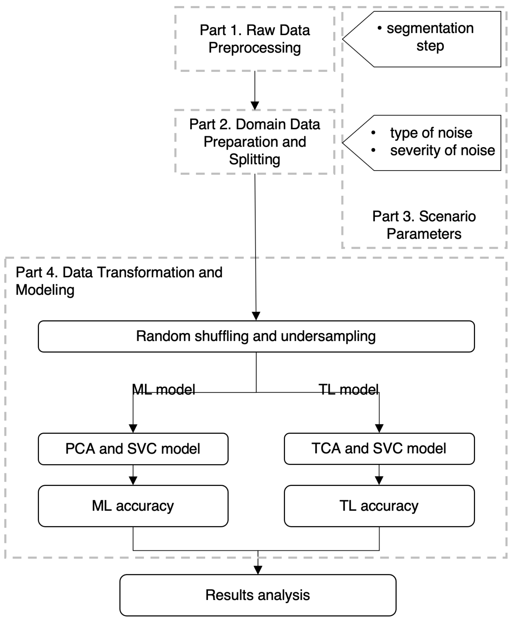
To compare the traditional ML approach with TL in the context of knowledge transfer from laboratory-recorded data (source domain) to an emulated workshop environment (target domain), a structured workflow was implemented. This workflow consists of four parts: raw data preprocessing, domain data preparation and splitting, scenario parameter variation, and feature extraction and modeling, as illustrated in Figure 2. Detailed explanations for each stage are provided in the corresponding subsections.

Binary classification was implemented to distinguish between balanced and unbalanced cases, with all unbalance levels grouped into a single class. In the modeling step, an ML model was developed and evaluated on the source-to-source transfer task, where both training and testing were performed using the source domain data. A TL model was then executed for the same task, and its classification accuracy was compared with that of ML models.

To assess model generalization, the ML and TL models were further evaluated on the source-to-target task, where training was conducted on the source domain data, whereas testing was performed on the target domain data. Model accuracy, sensitivity, and specificity were analyzed under different experimental conditions by varying three key parameters as follows:

• Segmentation step—influences the amount of training and testing data (Section 2.3.2);
• Type of added noise—represents ambient noise in a workshop environment, affecting the signal characteristics (Section 2.4.2);
• Severity of added noise—defines noise severity, simulating different levels of signal disruption under workshop conditions (Section 2.4.2).

These parameter variations resulted in 24 distinct preprocessing configurations, referred to as scenarios. The ML and TL models were executed for each scenario, with a detailed description of the parameters used in each scenario provided in Section 2.5.

2.3. Part 1: Raw Data Preprocessing

The preprocessing of the raw data, described in Section 2.1.2, consists of two steps: data exploration and cleaning and data segmentation (Figure 3). These steps were applied to both the development and evaluation datasets for all unbalance levels.

2.3.1. Data Exploration and Cleaning

Proper data cleaning is essential to ensure that model performance variations stem from actual model behavior rather than inconsistencies in data quality. Because this study evaluates performance under varying conditions, eliminating outliers prevents biases that could distort the results and ensures a fair comparison between ML and TL models.

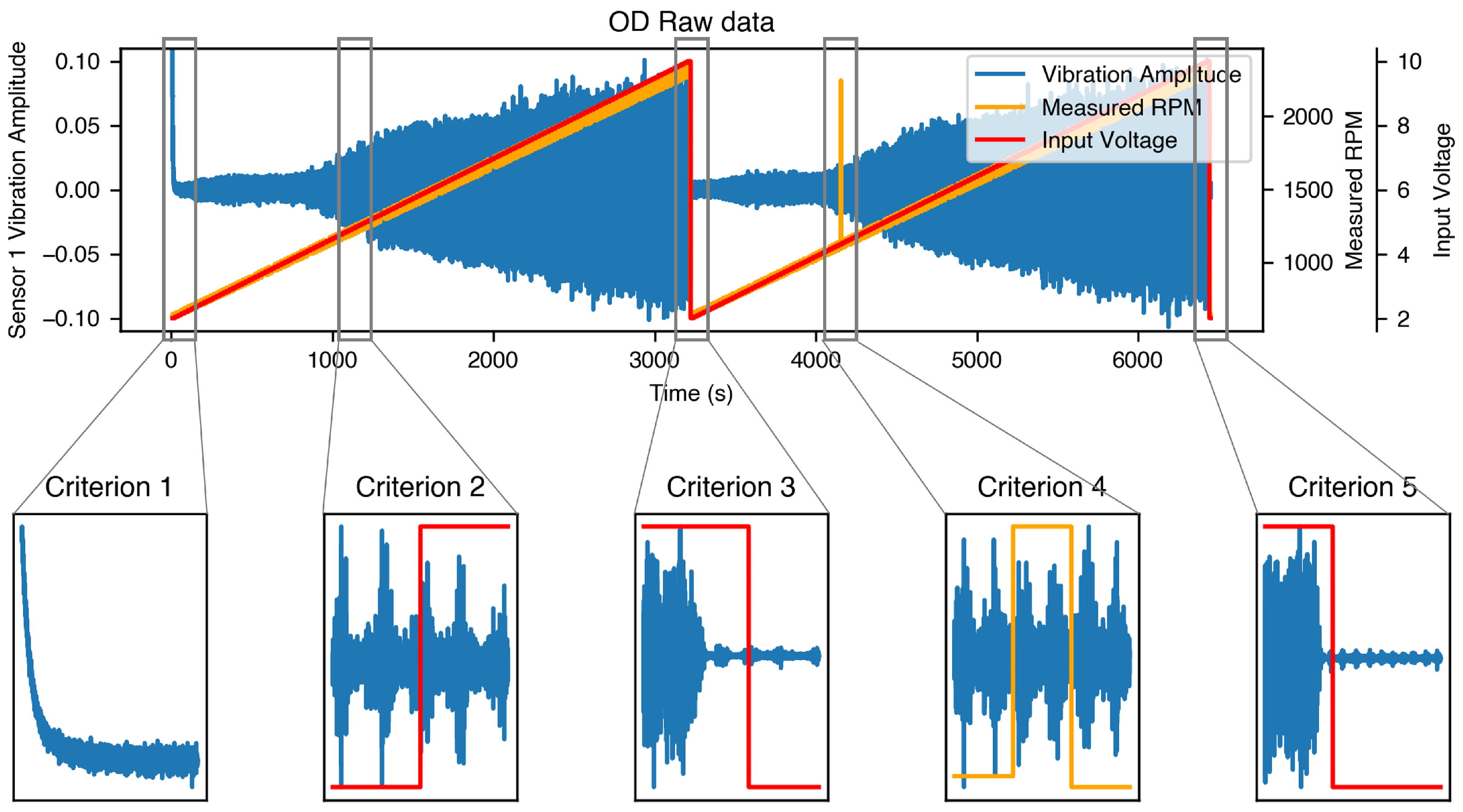
To achieve this, raw time-series data, including vibration signals and the corresponding voltage and speed values, were analyzed to detect distortions. Five criteria were established to identify unreliable data segments that were excluded from further analysis. Figure 4 presents an example recording of the development dataset with no added unbalance (0D) along with examples for each criterion, which are described below:

• Criterion 1: Beginning of recording. In [22], the authors recommended discarding the first 50,000 data points (approximately 10 s). However, data exploration revealed a longer unstable period, lasting up to 63 s in the development datasets and up to 43 s in the evaluation datasets. Because of the lack of detailed information on the recording procedure, the entire unstable segment at the beginning was considered distorted.
• Criterion 2: Voltage change. The data points recorded one second before and one second after each voltage change were affected by sudden speed fluctuations, leading to instability.
• Criterion 3: Cycle change. The data points recorded during the voltage drop between the two recording cycles were identified as being distorted.
• Criterion 4: Unexpected speed jumps. Sudden and unexplained speed jumps were observed in some of the datasets. Because these anomalies were not addressed in the data description, they were removed.
• Criterion 5: End of recording. Some recordings extended beyond the stop of rotation and speed drop, and these segments were excluded from analysis.

2.3.2. Data Segmentation

The raw data consisted of time-series recordings lasting several minutes. To prepare the data for modeling, data segmentation was performed on the cleaned vibration signal using a sliding window technique with no overlap. During this process, the entire recording was divided into continuous 1 s data samples, with a window shift equal to the Segmentation Step (Sstep). In this context, continuous means that if any portion of a 1 s sample was removed due to data cleaning criteria, the sample was considered incomplete and excluded from further processing. A 1 s window was selected to ensure sufficient temporal resolution for capturing unbalance-related vibration features across varying speeds. This duration provides enough data to capture several full shaft revolutions even at low speeds (300 RPM), enabling effective frequency-domain analysis. This choice is also consistent with prior vibration-based fault diagnosis studies, where 1 s segments are commonly used.

All the data samples generated using the same Sstep from the development recordings (0–4D) were combined into a single dataset. Samples from the balanced case (0D) were labeled as Class 0 (no unbalance), and samples from all unbalance levels (1–4D) were labeled as Class 1 (all unbalance levels), forming the preprocessed dataset D (Figure 3). The same process was applied to the evaluation recordings (0–4E), resulting in preprocessed dataset E.

The Sstep determines the amount of data extracted. Different Sstep were used across various scenarios, and details are provided in Section 2.5.

2.4. Part 2: Domain Data Preparation and Splitting

This section describes the data preparation process for the source and target domains and the train–test data split (Figure 3).

2.4.1. Data Splitting

Train and test data for the source and target domains were prepared as follows. For the source-to-source task, the entire preprocessed dataset D was used as the source domain train data, and the entire preprocessed dataset E without labels served as the source domain test data.

For the source-to-target task, the training data remained the same as in the source-to-source task using the source domain training data. The target domain data that mimicked various aspects of the production line were prepared by embedding synthetic noise into lab data samples. Since the target domain was used exclusively for testing, noise embedding was performed only on the preprocessed dataset E without labels, forming the unlabeled target domain test data (Figure 3). The process is described in the following subsection.

2.4.2. Noise Embedding

In a workshop environment, various ambient noises influence recorded data. The following are the most common types of disruptions in a production setting and the synthetic noise types used to represent them.

• White Gaussian Noise (WGN): Represents broadband random noise that introduces non-repetitive disturbances in the signal. This can arise from electronic interference, environmental factors, or other unpredictable disruptions in the measurement system [23].
• Electrical Noise (EN): A 50 Hz power line interference caused by electrical components and circuits in the surroundings [5].
• Impulse Noise (IN): Sudden, short-duration spikes or impulses in the signal, typically resulting from unexpected external impacts or mechanical shocks [24].
• Combined Noise (CN): A mixture of all the mentioned noise types, reflecting complex interference in a production environment [5].

To ensure noise variability, the synthetic noise samples were randomly regenerated for each data sample. This prevented the introduction of repetitive patterns into the simulated disruptions. Within the different scenarios, the effects of each noise type and their combination were analyzed under both weak and strong noise variations with characteristics selected through prescreening tests. Examples and exact characteristic parameters of the added noise across various scenarios are provided in Section 2.5.

2.4.3. Spectrum Creation

Since the rotor unbalance exhibits a clear pattern in the frequency domain, time-domain signal samples were transformed into spectra using a Fast Fourier Transform (FFT). Rotational speed was included as an additional scalar feature, concatenated to the FFT feature vector, providing context for learning speed-dependent vibration patterns.

2.5. Part 3: Scenario Parameters

Different scenarios were designed to systematically evaluate the model performance under varying conditions. These scenarios assess the impact of variations in factors such as noise type, severity, and data availability on both the ML and TL models. The complete set of parameters that varied across these scenarios is presented in

Table 2. Set of parameters varied across 24 investigated scenarios.

	Segmentation Step (Source and Target Domain Datasets)	Types of Noise (Target Domain Dataset)	Severity of Noise (Target Domain Dataset)
24 scenarios	10 × 4096 4 × 4096 1 × 4096	Gaussian White Noise Electrical Noise Impulse Noise Combined Noise	Weak Strong

.

2.5.1. Data Availability

Three data availability levels, controlled by Sstep size, were examined across the scenarios.

• Sstep = 1 × 4096: The segmentation window moved forward every second (equal to the sampling frequency), ensuring consecutive, non-overlapping samples and utilizing 100% of the available data. This resulted in a development dataset containing 5409 samples for Class 0 (no added unbalance) and 21,612 samples for Class 1 (all unbalance levels combined), while the evaluation dataset contained 1382 samples for Class 0 and 5521 samples for Class 1.
• Sstep = 4 × 4096: The segmentation window was moved by 4 seconds, introducing a 3 s gap between consecutive samples and reducing data utilization to 25%.
• Sstep = 10 × 4096: The window moved forward by 10 s, creating a 9 s gap between samples and utilizing only 10% of the available data.

The selection of data availability levels (10%, 25%, and 100%) was based on the typical learning curve behavior of traditional ML models, where accuracy increases rapidly between very low to moderate data availability but gradually plateaus as more data are added. This choice captured the critical improvement phase, enabling a comparison of the accuracy trends between the ML and TL models under varying data constraints. The exact number of data samples generated by the different Sstep are summarized in

Table 3. Segmentation step (Sstep) and amount of generated data samples per recorded dataset, the total amount of data used per class for binary classification, and % of data utilized for each Sstep.

Sstep × 4096	Amount of Data Samples Created per Dataset					Total per Class (D/E)		% of Utilized Data
	0D/0E	1D/1E	2D/2E	3D/3E	4D/4E	Class 0	Class 1
10	479/123	562/123	584/123	579/123	593/123	479/123	2318/492	10%
4	1273/325	1467/325	1273/324	1459/325	1436/325	1273/325	5635/1299	25%
1	5409/1382	5400/1381	5409/1378	5403/1381	5400/1381	5409/1382	21,612/5521	100%

.

Since the same speed was maintained for 20 s during the two recording cycles, the number of samples per speed level varied with Sstep. With Sstep = 1 × 4096, a maximum of 40 samples per speed level were generated, whereas with Sstep = 10 × 4096, only 4 samples per speed were possible. The actual number of samples could be lower if some of them were considered incomplete and excluded due to data cleaning criteria (Section 2.3.1).

2.5.2. Severity and Types of Noise

Both strong and weak versions of each noise type were embedded in the raw signal samples in different scenarios. The specific settings used for noise generation were as follows:

• Weak WGN: The Mean was set to 0, and the Standard Deviation was 0.005. Strong WGN: The Mean was 0, and the Standard Deviation was 0.01.
• Weak EN: Amplitude was 0.005. Strong EN: Amplitude was 0.02.
• Weak IN: The number of impulses was randomly selected between 1 and 5, and the Amplitude Range was between 0.05 and 0.1. Strong IN: The number of impulses was randomly selected between 3 and 8 and the Amplitude Range was between 0.1 and 0.2.
• Weak and Strong Variants of CN: Combination of WGN, EN, and IN at their respective weak or strong levels.

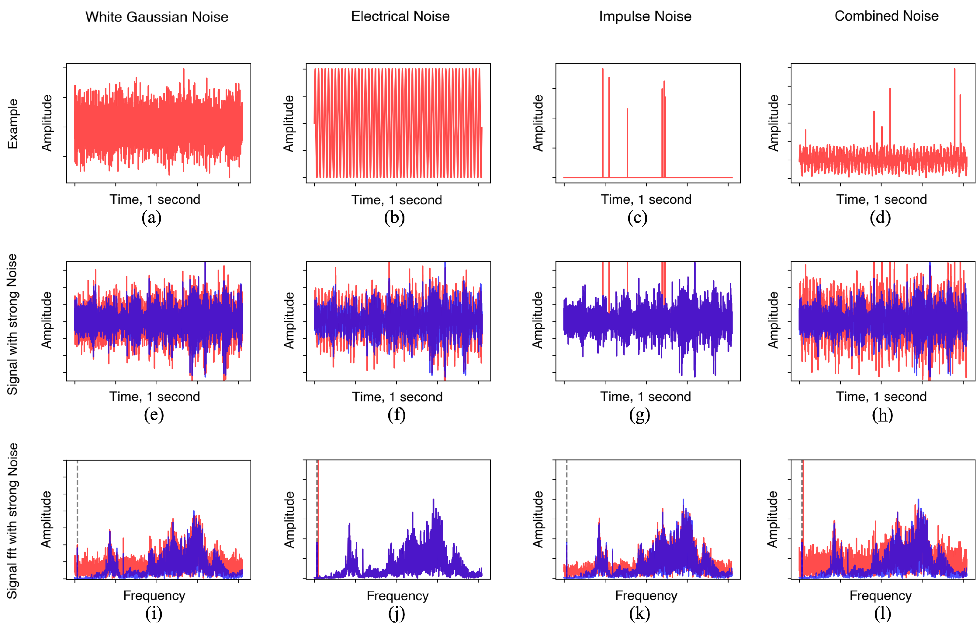
The parameters for generating weak and strong noise variations were determined through a preliminary prescreening process aimed at defining meaningful boundaries of noise severity for model evaluation. For each noise type, a range of parameter values was systematically tested to identify a lower threshold where noise began to degrade accuracy and an upper threshold beyond which classification became unreliable. Additionally, selected parameters were required to result in classification accuracies for both ML and TL models within an interpretable range of approximately 50% to 95% across all Combined Noise scenarios. This process also revealed which noise levels had negligible impact and which exceeded model capacity, providing a practical basis for defining weak and strong noise settings for analysis across scenarios. Examples of the generated noise signals, vibration signals with embedded strong noise, and their spectra are shown in Figure 5.

2.6. Part 4: Features Preparation and Modeling

The prepared source and target domain datasets were used for binary classification, where Class 0 represented balanced bearing cases and Class 1 included data from four rotor unbalance levels. This resulted in an imbalanced dataset, with Class 1 containing four times more samples than Class 0. Since maintaining a balanced dataset is crucial for reliable model performance, data balancing was performed on Class 1 using an undersampling technique [25].

It is important to distinguish between the terms “balanced” and “unbalanced” when referring to bearing conditions and dataset structure, as “balanced and unbalanced bearing” describes the mechanical state of the system, while “balanced and imbalanced dataset” refers to the class distribution in model training.

Random shuffling was applied to the dataset before undersampling to minimize potential bias. The undersampling process could skew the proportion of low- and high-level unbalance samples in the training and test sets, potentially affecting the model performance. Lower-level unbalance is generally more challenging to detect, and model performance could decline if the training set contained fewer low-level unbalance samples, whereas the test set had more.

To ensure comparability across scenarios, random sampling was performed once within the same Sstep, and the resulting datasets were used consistently for both the ML and TL models across all scenarios for that Sstep. This approach prevents unnecessary variability within scenarios and ensures fair performance comparisons between different noise conditions.

For classification, a Support Vector Machine (SVM) algorithm was selected for both the ML and TL models due to its strong performance in traditional ML and TL applications [26]. The SVM classifier relies on several key hyperparameters: the kernel function, the regularization parameter C, and the kernel coefficient gamma. The kernel determines how input data are mapped into a higher-dimensional space for non-linear classification; options evaluated during a grid search included linear, polynomial, and radial basis function (RBF) kernels. The regularization parameter C, tested with values [0.1, 1, 10], controls the trade-off between margin maximization and training error minimization. The kernel coefficient gamma, which influences the reach of individual training samples, was tested using “scale” and “auto” settings. Higher values of C and gamma tend to create more complex decision boundaries, which may increase training accuracy at the cost of generalization.

All three parameters were optimized using grid search with 5-fold cross-validation on the development dataset (preprocessed Dataset D) for the source-to-source task with 100% data availability. The optimal configuration—RBF kernel with C = 10 and gamma set to “auto”—was selected based on the best average validation accuracy. This configuration achieved a balance between model complexity and generalization capability. To ensure consistent and fair comparisons between ML and TL models, these hyperparameters were kept fixed across all evaluated scenarios.

Additionally, the number of dimensions for the FFT-based feature vectors was determined through empirical evaluation. Various dimensionalities were tested, and 30 components were selected as a trade-off between preserving informative variance and avoiding overfitting. This dimensionality was applied consistently across all experiments.

In the traditional ML approach, Principal Component Analysis (PCA) was applied for feature transformation from the FFT-transformed data samples, retaining a 30-dimensional feature space. The Support Vector Classifier (SVC) model was then trained on the source domain train data and evaluated in two steps:

• source-to-source task: The trained model was tested on the source domain test data.
• source-to-target task: The same trained model was tested on the target domain test data across all scenarios.

For the TL approach, a distance-based domain adaptation technique called TCA was applied for feature transformation from the FFT-transformed data samples, reducing them into a 30-dimensional latent feature space [7]. The process is as follows:

• Source-to-source task: TCA was first applied to map the source training and source test data into the same latent space. An SVC model was then trained on the transformed source training data and evaluated using the transformed source test data.
• Source-to-target task: TCA was used to project the source training and target test data into the shared latent space. The SVC model was trained on the transformed source training data and tested on the transformed target test data for various scenarios.

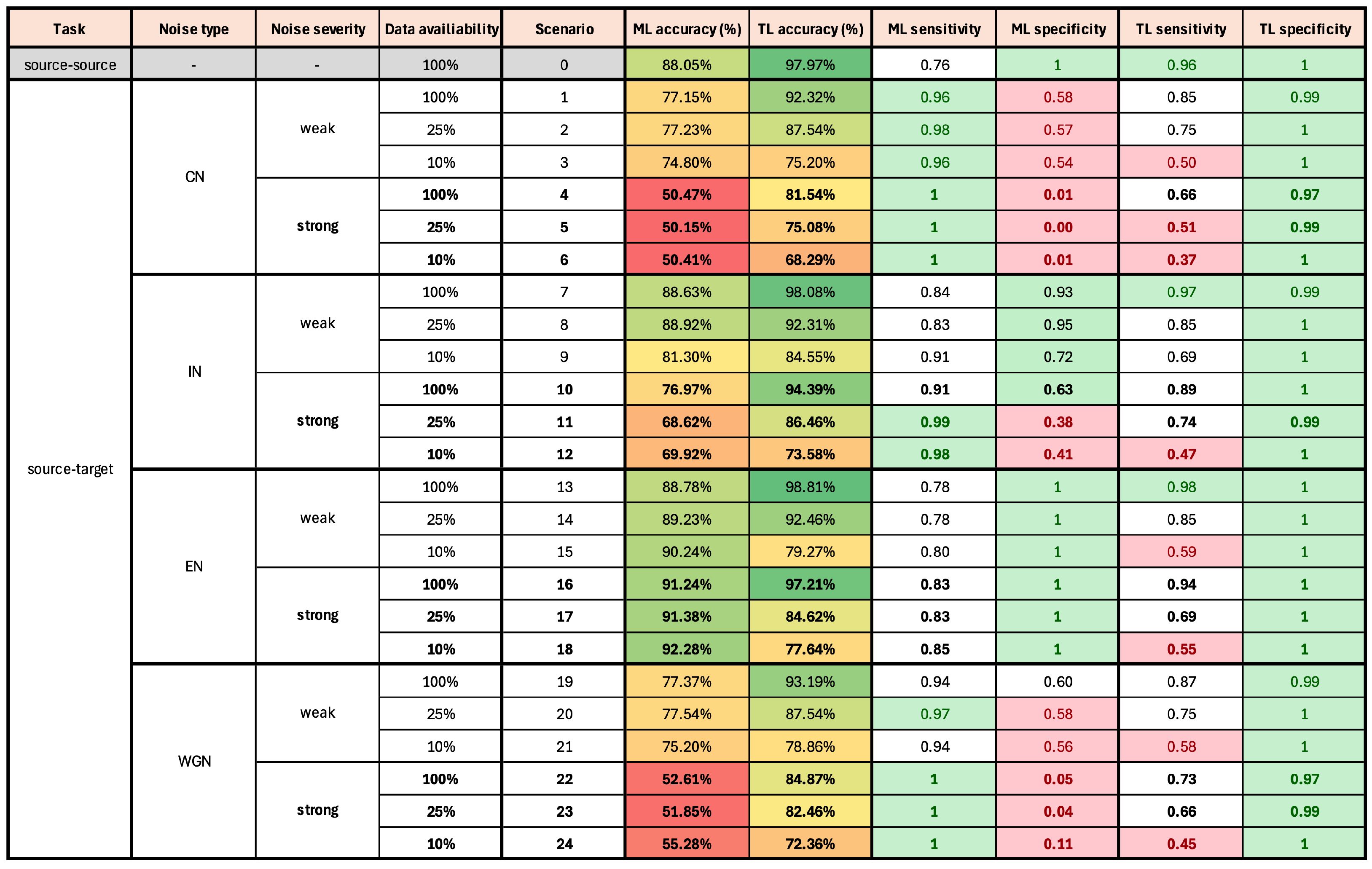
Figure 6 presents the classification results for different scenarios. Additionally, for each scenario, sensitivity and specificity values were calculated for both ML and TL models to provide a more comprehensive performance analysis.

3. Results and Discussions

The results across various scenarios were evaluated by considering the effects of data availability, noise type and severity, rotational speed variations, and unbalance levels. This provides a comparative assessment of both models, offering insights into their strengths and limitations under different conditions.

The overall results are presented in Figure 6, with detailed explanations and discussions in the following subsections. The table includes classification accuracy, sensitivity, and specificity values for both the ML and TL models across all investigated scenarios. Accuracy levels are color-coded, with red indicating the lowest values and green the highest. Sensitivity and specificity are also highlighted for a more straightforward interpretation, with green denoting values above 0.95 and red ones below 0.6. Scenarios are grouped by noise type, with bold font indicating strong noise cases and regular font indicating weak noise cases. Scenario Zero, highlighted in gray, serves as the baseline (source-to-source transfer), while the remaining scenarios correspond to source-to-target transfer tasks.

Key observations from the results indicate that the TL model consistently outperforms the ML model, achieving a higher classification accuracy across most of the investigated scenarios. The ML model performed particularly poorly in cases with CN and WGN, demonstrating its susceptibility to noise disruptions, especially in the case of strong noise severity. The TL model exhibited exceptionally high specificity, effectively identifying non-faulty cases.

3.1. General Results

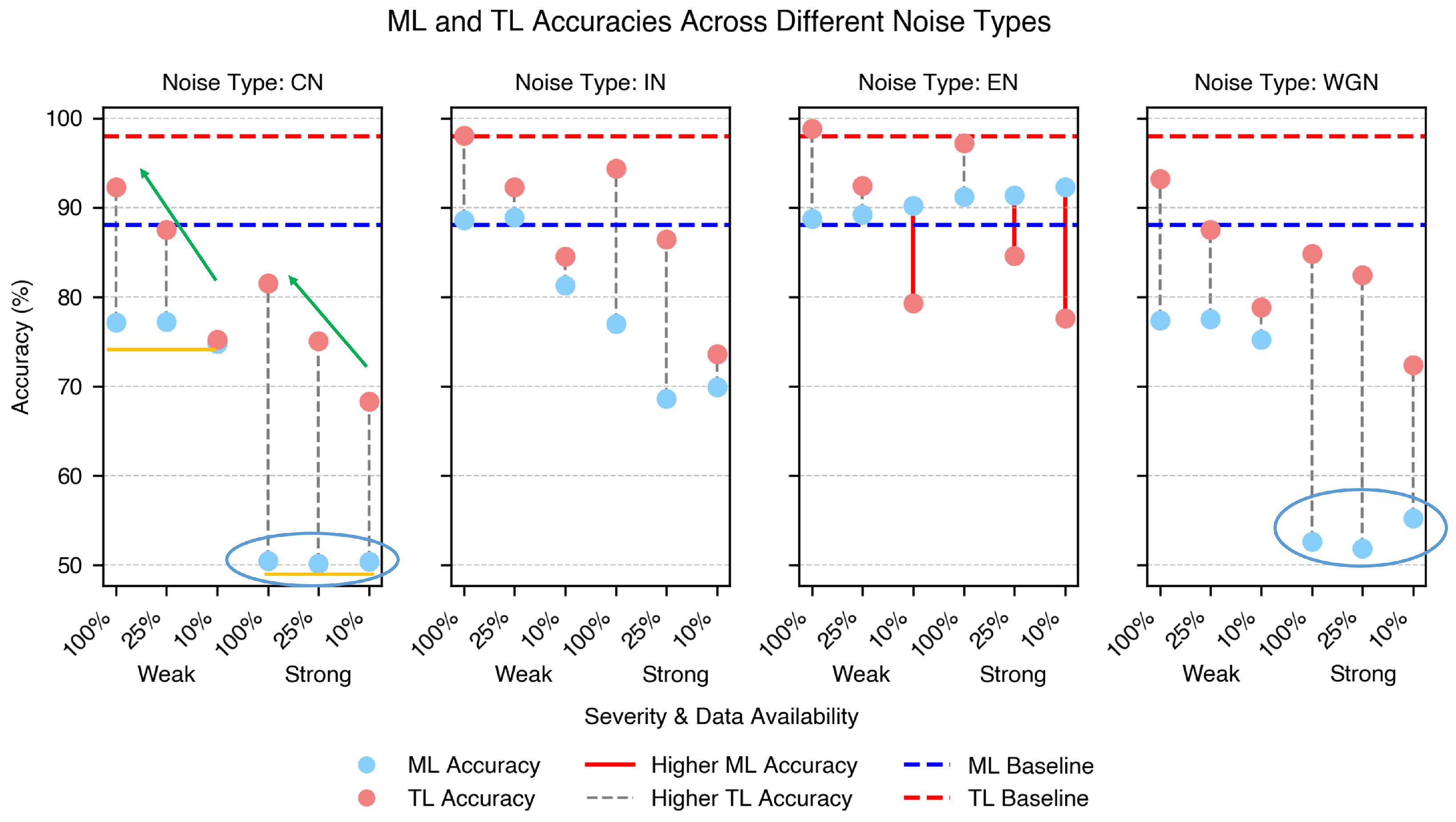
The classification accuracies for all source-to-target transfer scenarios are shown in Figure 7. For the baseline Scenario Zero, the ML accuracy is shown by the blue horizontal dashed line, and the TL accuracy is shown by the red dashed line.

Overall, the TL model achieved significantly higher classification accuracy than the ML model, with improvements exceeding 30% in some cases, such as in the strong CN scenario with 100% data availability. The grey dashed vertical lines indicate the accuracy difference between the ML and TL models within each scenario where TL performed better. There are three exceptional cases in which the ML model performs better than the TL model, marked by red vertical lines. These correspond to the EN scenarios. In these cases, the ML model performed better than the TL model, particularly under low data availability conditions.

The better performance of the ML model compared to that of the TL model in the presence of EN may be attributed to the distinct frequency-domain pattern of EN (Figure 5j). Since the ML model processes features extracted directly from the frequency domain after dimensionality reduction, this pattern might remain prominent in the input data, allowing the model to leverage it for classification. In contrast, the TL model transforms frequency-domain data into a common latent space to align the source and target distributions. This transformation may obscure or weaken the distinct characteristics of EN, making it less distinguishable and potentially reducing the classification performance. Nevertheless, since EN are easy to detect and remove through signal processing, these cases are not critical from a practical standpoint.

The weakest ML performance was observed in scenarios with strong WGN and CN, as highlighted by the light blue circles in Figure 7. The TL model significantly enhances the classification accuracy in these cases. Notably, the ML and TL models exhibit nearly identical performances for the WGN and CN. This finding was unexpected, as CN, which combines multiple noise types, was supposed to have a more substantial negative impact.

IN has a minimal effect on both ML and TL models compared to the baseline performance, particularly in its weak form when data availability is high. When 100% of the data are available, the TL model handles even strong IN effectively, whereas the ML model experiences a significant drop in accuracy.

Data availability plays a crucial role in TL model performance across all noise types, with increased data significantly improving the accuracy. Examples of this trend are highlighted by green arrows in Figure 7 CN. In contrast, the ML model remains largely unaffected by data availability, maintaining stable accuracy across different data volumes, as shown by the yellow horizontal lines in the same subfigure. This indicates that, in most scenarios, the TL model can achieve an accuracy comparable to that of the ML model with significantly less data. This advantage highlights the ability of the TL model to leverage domain adaptation for improved generalization, making it a viable approach in data-limited industrial applications.

Furthermore, the results suggest that the accuracy improvement of the ML model plateaued at a data availability level below 10%, indicating that additional data beyond this threshold did not contribute to further performance gains. Conversely, the TL accuracy continued to improve at 100% data availability, implying that TL models may achieve even higher accuracy with greater data availability.

The impact of noise severity on the model performance is evident across most noise types, where stronger noise generally leads to lower accuracy. However, EN is an exception, as model performance remains unaffected by the increase in noise levels.

For both the ML and TL models, Scenario Zero usually achieved the highest accuracy. However, the TL model surpasses the baseline of the ML model in several cases, demonstrating its effectiveness in transferring a model trained on lab-recorded data to an emulated workshop environment.

3.2. Classification Accuracy Improvement per Noise Type

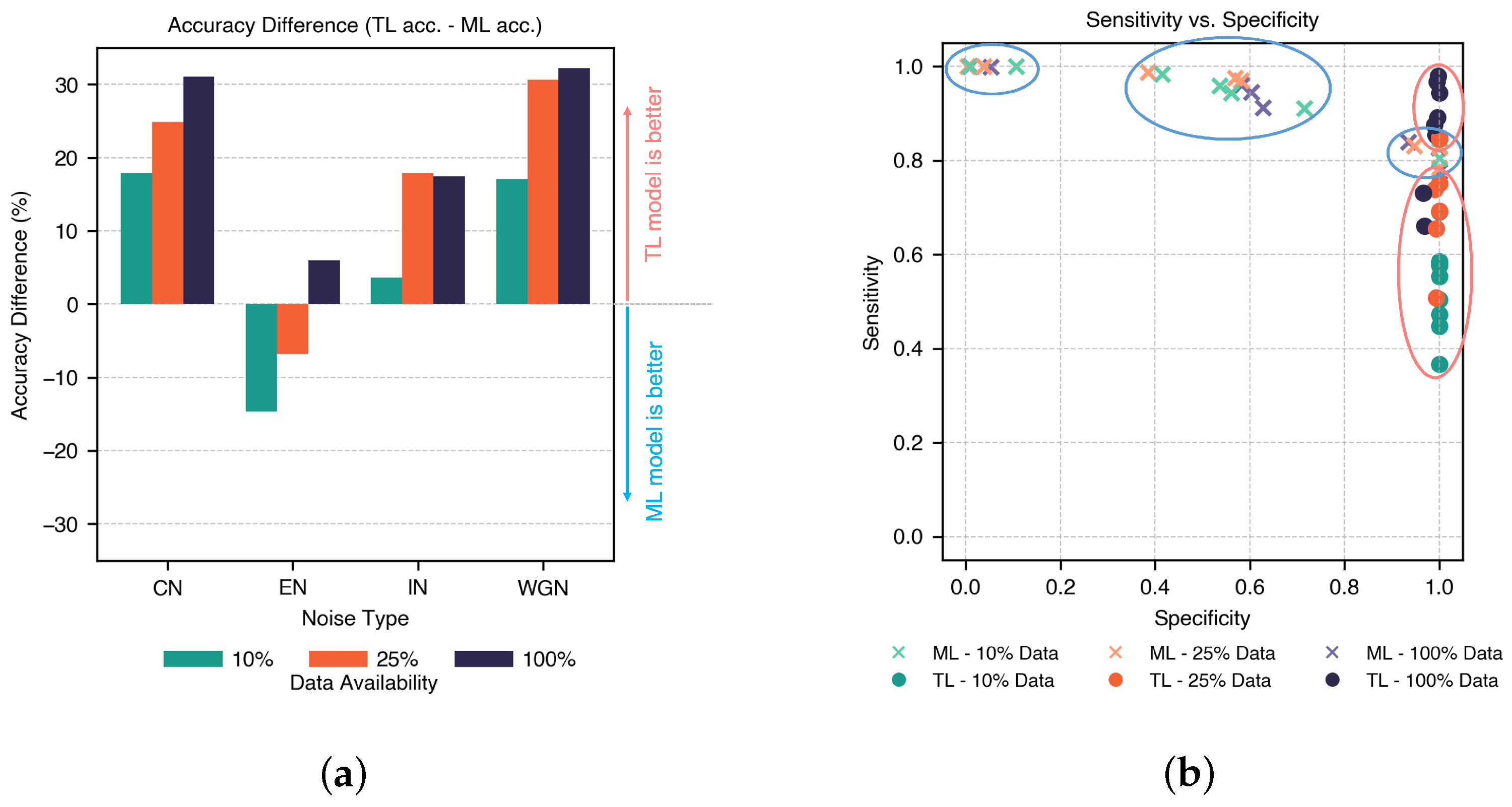
The accuracy differences between the TL and ML models for strong variants of all types of noises across different data availabilities are illustrated in Figure 8a, representing the range of TL accuracy minus ML accuracy. This difference is positive when TL outperforms ML, and negative when ML performs better.

The results indicate that TL consistently outperformed ML in most scenarios, except for EN under low data availability. The most substantial TL improvements were observed in scenarios with larger datasets affected by WGN and CN and reached above 30%. This suggests that TL benefits the most from greater data availability and complex noise environments. This highlights the ability of the TL to generalize under noisy conditions where ML struggles.

3.3. Sensitivity vs. Specificity

The results in Figure 6 indicate that the TL model consistently achieved high specificity across all scenarios, which means that it is more effective at correctly identifying true negative cases (absence of unbalance). In contrast, the ML model exhibits stronger sensitivity and is better at detecting true positive cases, particularly under specific noise conditions.

To further investigate this trade-off, Figure 8b compares the sensitivity and specificity of the ML and TL models across different scenarios. The color scheme represents data availability, with ML values shown as cross markers enclosed in blue ovals and TL values shown as circle markers in red ovals. Figure 8b illustrates that the ML model consistently achieved high sensitivity, but its specificity varied widely across scenarios without a clear pattern. In contrast, the TL model maintains high specificity, with sensitivity improving as data availability increases, as indicated by the upward trend of TL markers in blue compared to green, with orange in between. Notably, only a few ML cases achieved high specificity at the cost of a lower sensitivity.

3.4. Correct Predictions per Unbalance Level

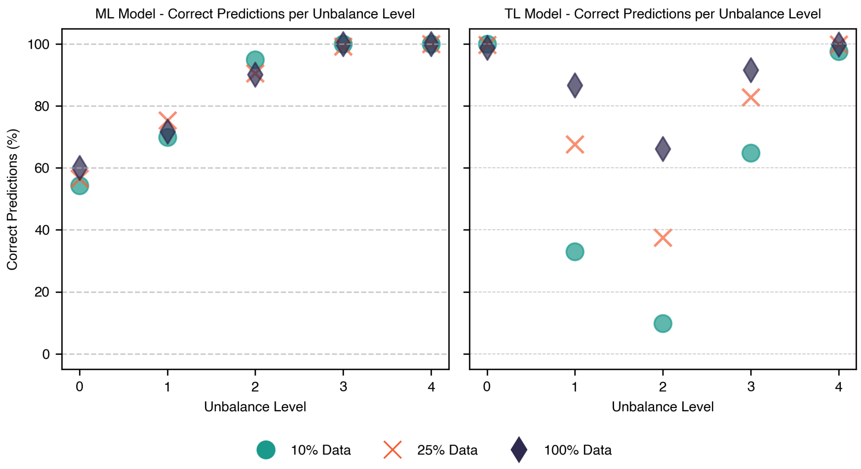
Expanding on the sensitivity and specificity analysis, Figure 9 provides a detailed comparison of the classification accuracy across different unbalance levels for both the ML and TL models. The y-axis represents the percentage of correctly classified samples per unbalance level under various data availability conditions. These values were calculated by dividing the number of correctly predicted samples for each unbalance level within the same data availability condition by the total number of samples in the group. Each unbalance level is represented by three points on the y-axis, corresponding to the high (100%), low (25%), and lowest (10%) data availability.

The ML model maintained over 60% accuracy across all unbalance levels and exceeded 90% for levels 2, 3, and 4. In contrast, the TL model exhibits greater variability, with accuracy dropping to approximately 10% for unbalance Level 3 under low data availability but improved significantly with more data, achieving up to a 60% increase. While the ML model reaches relatively stable accuracy levels across different data conditions, its overall accuracy is lower due to the high misclassification rate for balanced cases. This occurred because the dataset was balanced; the number of samples for Level 0 equaled the combined samples of all other levels, amplifying the impact of misclassified balanced cases on the overall ML accuracy.

These findings align with the sensitivity vs. specificity analysis and highlight the need for further fine-tuning the TL model to enhance performance in borderline unbalance conditions, especially under data constraints. One possible improvement is to treat each unbalance level separately through multi-class classification or domain adaptation techniques tailored to specific unbalance levels. This would allow the model to learn more precise decision boundaries and better capture small differences between unbalance levels, especially for early-stage faults like Level 1. In addition, future work could explore stratified sampling techniques to ensure balanced representation of all unbalance levels during training, and metric learning approaches (e.g., triplet loss or contrastive learning) to improve feature separability. Despite some limitations, the TL model consistently achieved a higher classification accuracy than the ML model, reinforcing its suitability for condition-based maintenance applications.

3.5. Correct Predictions per Recording Sample

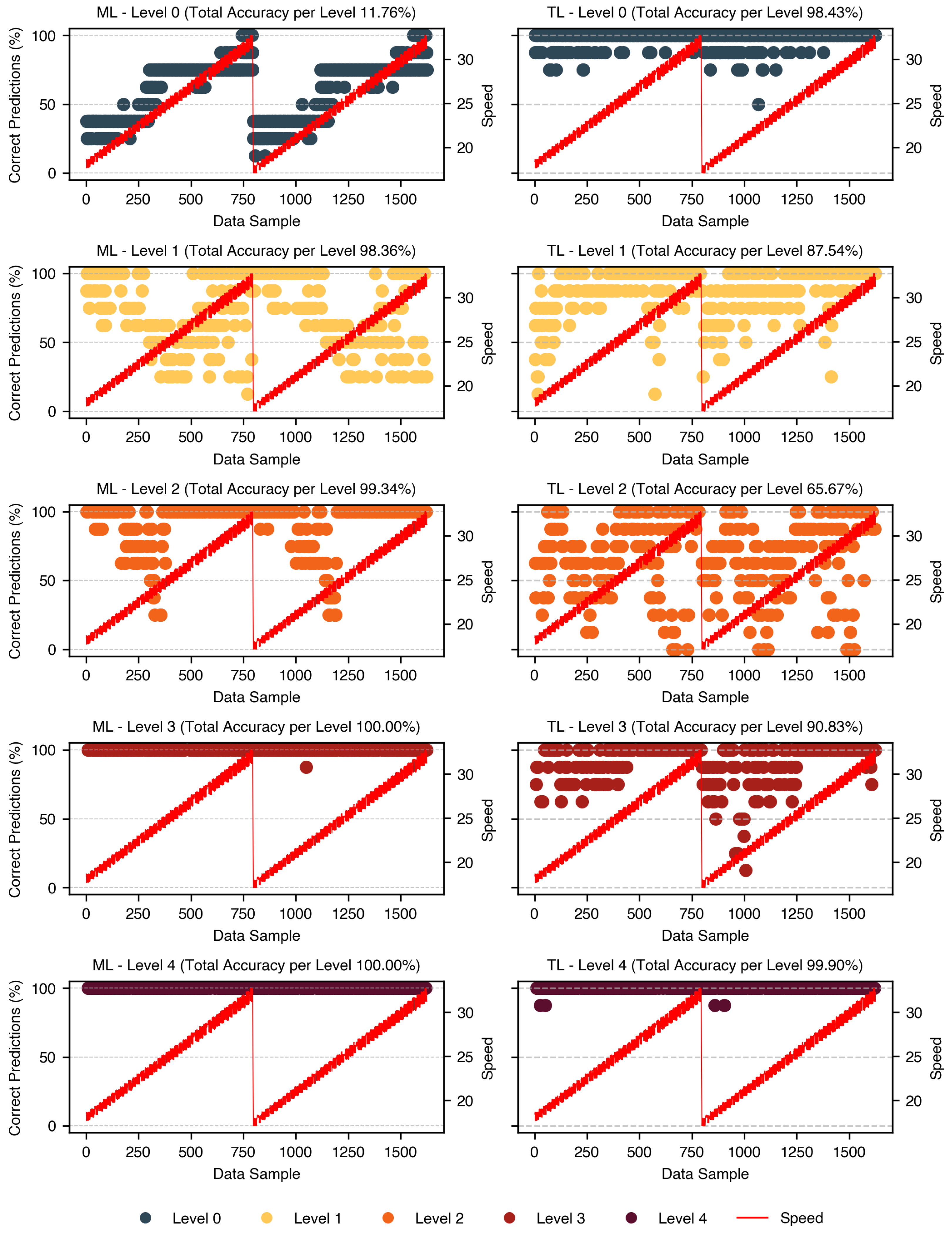
Understanding how classification performance varies across different operational speeds and unbalance levels is crucial for assessing the model’s effectiveness. Figure 10 illustrates the percentage of correct predictions per data sample across different speed levels for the scenarios with the highest data availability. These values were calculated separately for each unbalance level, providing a detailed comparison of model performances.

For the ML model, correct identification of the balanced class improved as speed increased, aligning with expectations. The Signal-to-Noise Ratio (SNR) decreases at higher speeds, making unbalance patterns more distinct and easier to detect. Additionally, unbalance effects become more pronounced at higher speeds due to increased centrifugal forces, further improving the pattern visibility and model learning. However, level 1 follows the opposite trend, with the accuracy decreasing as speed increases. This effect requires further investigation. Level 2 performs particularly poorly within the 1200–1400 RPM range but significantly improves beyond this threshold, suggesting a possible resonance effect. Levels 3 and 4 achieved near-perfect accuracy, maintaining close to 100% correct predictions across all speed levels.

For the TL model, balanced cases were consistently well classified across all speeds. Level 1 shows a positive correlation with speed, with accuracy increasing at higher speeds, whereas Level 2 remains relatively stable across different speed levels. Level 3 demonstrates a marked improvement beyond 1400 RPM, whereas Level 4 maintains high accuracy across all speeds with no significant impact from speed variations.

These findings highlight the strong influence of speed on the classification accuracy of the ML model, where higher speeds improve the detection of both balanced cases and severely unbalance levels. In contrast, the TL model demonstrated greater stability across speeds, with classification accuracy more dependent on unbalance levels than speed variations.

4. Conclusions

This study evaluated the ability of TL models to address the generalization challenges of traditional ML models when transferring AI models trained on lab-recorded data to an emulated workshop environment with varying operational conditions. The case study focuses on detecting rotor unbalance across different speed variations and provides insights into the strengths and limitations of traditional ML and TL models. The classification accuracy, sensitivity, and specificity were analyzed across multiple scenarios, considering the effects of data availability, noise type and severity, rotational speed variations, and different unbalance levels.

The results demonstrate that the TL model outperforms the ML model, particularly in source-to-target tasks with high data availability, achieving up to a 30% accuracy improvement in complex noise environments such as WGN and CN. While ML effectively detects unbalanced conditions, it often misclassifies balanced cases. TL maintains strong unbalance detection but struggles with mild unbalance levels, particularly under limited data conditions. The ML accuracy remains stable across different data availability levels, whereas TL showed continued improvement with more data.

This study also highlights the influence of noise type, severity, and speed variations. The WGN and CN presented the greatest challenges for both models, but TL exhibits greater robustness. ML benefits from higher speeds achieving better classification results for high RPM samples, while TL remains stable across different speed conditions, with accuracy primarily dependent on unbalance levels rather than speed.

The ML accuracy improvement curve plateaus below 10% data availability, with no further gains beyond this threshold. In contrast, TL accuracy continued to improve at 100% data availability, suggesting the potential for even higher performance with more data.

These findings emphasize the ability of the TL to generalize to noisy environments and adapt to complex conditions, reinforcing its potential for real industrial applications. It is important to highlight that classification accuracy alone is an insufficient metric for assessing real-world effectiveness. As demonstrated in this study, a comprehensive evaluation of model performance is crucial for enhancing the reliability and improving the diagnostic capabilities of TL models.

In terms of practical application, the proposed method is computationally efficient and suitable for real-time analysis using 1-second data segments, making it feasible for industrial settings where continuous monitoring may be constrained by operational limitations or sensor accessibility. However, the current model was trained on a single bearing geometry and fault type, which limits its generalizability to other use cases. To develop a broadly applicable system, future work should incorporate data from diverse bearing types and failure modes. While this study did not aim to build a general-purpose diagnostic tool, it provides a structured analysis of how key parameters influence TL performance.

The presented results were based on a case study of rotor unbalance identification through bearing vibration signals. However, the insights gained from this study can be used beyond this specific application. The findings on TL’s effectiveness and limitations in handling domain shift may offer valuable guidance for investigating other bearing failure modes, such as inner and outer race defects or rolling element damage. Additionally, these insights can contribute to more detailed studies on fault detection in other rotating machinery applications, including gearbox failures, motor faults, and similar industrial maintenance tasks where data scarcity and domain adaptation remain significant challenges. The proposed methodology can be applied to assess the impact of other influencing factors, such as outliers in the data and variations in the sensor placement, which affect the recorded data characteristics.

Future work should focus on improving the sensitivity of TL models, particularly for detecting mild unbalance levels. Exploring multi-class classification, where unbalance levels are treated as distinct categories rather than a single class, can provide a more detailed classification framework and improve detection accuracy. Examining the influence of sensor placement on model performance can provide valuable insights, particularly given practical constraints in industrial settings where optimal sensor positioning is not always feasible. Additionally, investigating tailored domain adaptation techniques and refined preprocessing strategies may further optimize the TL performance. Leveraging more advanced TL methodologies could further enhance model generalization and improve their applicability in real-world industrial settings.