Methodology for Implementing Monitoring Data into Probabilistic Analysis of Existing Embankment Dams

Abstract

Monitoring data provide valuable information on embankment dam behavior but are typically not integrated into a classical probabilistic safety assessment. This paper introduces a Bayesian-inspired methodology to directly integrate actual dam monitoring records into a Monte Carlo probabilistic safety assessment using a finite element framework, without recalibrating the original input parameters ‘distributions. After the baseline (unweighted) set of simulations is generated, the method assigns a weight coefficient to each simulation outcome based on the likelihood of matching monitoring data, effectively updating the baseline probabilistic analysis results. Therefore, such “weighted” analysis produces an updated probability distribution of the dam’s factor of safety (FS) that reflects both prior uncertainty of model parameters and actual monitoring data. To illustrate the approach, a case study of a rockfill triaxial test specimen is analyzed: a baseline probabilistic analysis yields a mean FS ~1.7, whereas the weighted analysis incorporating monitoring data reduces the mean FS to ~1.5 and narrows the variability. The weighted analysis suggests less favorable conditions than the baseline projections. This methodology offers a transparent, computationally tractable route for embedding monitoring evidence into reliability calculations, producing more reflective safety estimates of actual dam behavior.

1. Introduction

Embankment dams are hydraulic structures constructed from natural materials available near the construction site. Depending on the type of material used, they may be classified as earthfill dams (with either homogeneous or heterogeneous cross-sections) or rockfill dams. According to ICOLD data [1], there are over 58,000 high dams worldwide, of which approximately 75% fall into the category of embankment dams. The safety assessment of such dams is a critical issue due to the potentially catastrophic consequences that a failure could entail, both in terms of human lives and economic losses.

In the broadest sense, the failure of an embankment dam represents a catastrophic scenario in which the structure is unable to withstand the applied loads, leading to at least one of the following incidents: the uncontrolled release of reservoir water or a complete loss of structural integrity of the dam and/or its foundation.

It is clear that the embankment dams (due to their large size, complex geotechnical conditions, and the potentially catastrophic consequences of failure) are structures characterized by a very high level of risk. As outlined in Eurocode 7 [2], they fall under Geotechnical Category 3, which demands in-depth investigations and advanced engineering practices. ICOLD standards further highlight the necessity of ongoing monitoring and risk evaluation to ensure the safety and performance of these critical infrastructures.

ICOLD in its Bulletin 154 [3] states the following principle: “The fundamental dam safety objective is to protect people, property and the environment from harmful effects of mis-operation or failure of dams and reservoirs. Accordingly, a dam must have an acceptable level of safety at all times”. For that reason, one of the most important activities in dam-safety management, both for existing dams and during the design phase, is the continuous safety review. The ICOLD Bulletin 154 [3] states that the safety review must provide an answer to the question “Does the dam system conform to current regulatory requirements, current national and international standards and practices, and to current requirements with respect to acceptable and tolerable risk criteria?”.

Analyzing its behavior and assessing the safety of a dam rely on conducting computational simulations of relevant physical processes, which are most commonly performed using the finite element method (FEM). Material parameters that serve as an input for a FEM model are most often derived from two primary sources of known (measured) data: preliminary investigation and monitoring data. The preliminary investigation typically includes results from laboratory testing and in-situ experiments conducted during the design or investigation phases, which provide insight into the behavior of individual materials usually on a much smaller scale compared to the structure as a whole. Nevertheless, these tests are very useful, as they provide engineers with a certain understanding of material behavior in controlled conditions.

The long-term safety of a dam depends as much on systematic monitoring during its operation as on a sound design and construction. The data monitored on dams directly reflect the structure’s response to external actions, revealing both its overall displacements, and the changes in its internal seepage and stress–strain state. ICOLD Bulletin 154 [3] emphasizes that the operational phase poses the greatest safety challenge and therefore requires a structured management system in which monitoring data are collected (automatically or manually), checked and interpreted in a timely manner to support risk-informed decisions. Each monitoring scheme is unique, tailored to a particular dam of a particular structural type and foundation setting.

The dam’s response that is being captured by monitoring data is inherently stochastic. Recognizable trends within the dam’s behavior do exist, yet the complex interplay of variable external loads and the structure’s non-linear response mean that nominally similar conditions rarely yield identical readings. Further scatter in monitoring data arises from instrument precision limits, measurement error and data-handling noise. Consequently, the monitoring observations should be treated as random variables and described by appropriately assigned probability distributions, not as single deterministic values. Finally, not all types of monitoring data carry the same level of reliability or significance [4]. Certain instruments provide more accurate or consistent measurements than others, and some monitoring points are more critical due to their location or relevance to the dam’s behavior. As a result, the interpretation of monitoring data should consider the contextual importance of each measurement point.

Methods for the safety assessment can be deterministic and probabilistic, where these terms illustrate the treatment of model input variables in calculations. The deterministic approach is the traditional way of solving safety problems, where the computational parameters of materials and/or loads and hydraulic boundary conditions are defined as constant values. Many current design codes still prescribe deterministic safety criteria expressed through minimum factors of safety (FS). These requirements are rooted in long-standing engineering practice and empirical experience. Although widely used in design and evaluation, the global factor of the safety approach has inherent limitations: it neither distinguishes among different sources of uncertainty nor provides a direct estimate of failure probability.

By the second half of the twentieth century, the dam-engineering community recognized the need for a systematic treatment of uncertainty. The arrival of probability theory and structural reliability concepts opened the door to a broad family of probabilistic analysis methods [5]. These methods model the stochastic behavior of key variables and deliver measurable quantities such as the probability of failure (p_f) and the reliability index (β), which can be compared with target values specified in reliability-based standards. ISO guidelines [6] and Eurocodes [7] now define target β-values that structures must meet.

Numerous studies have expanded the reliability assessments of dam and slope stability by incorporating advanced probabilistic methods into conventional analysis frameworks [8,9,10,11,12,13,14,15,16,17,18,19,20,21], but these efforts generally overlook the incorporation of actual dam monitoring data. The problem of integrating the monitoring data into the analysis has been addressed theoretically in several works [22,23], in which it is either treated deterministically, or, in the case of a probabilistic attempt, by using full Bayesian updating. The examples of using the Bayesian updating approach have been reported for smaller or less-complex geotechnical systems such as landslides and rock slopes [24,25,26,27,28,29,30]. For large embankment dams, whose instrumentation produces high-dimensional stochastic data, a full Bayesian integration is very computationally challenging [31]. Several studies have explored techniques to reduce the computational burden, including surrogate modeling approaches or reduced-order models in geotechnical problems [17,28,29].

This paper introduces a methodology that implicitly integrates monitoring data, with their inherent stochastic character, directly into a Monte Carlo probabilistic safety assessment. Although this methodology is developed in the context of embankment dam safety, its applicability extends to other geotechnical systems where systematic long-term monitoring is implemented (e.g., the safety assessment of large natural or engineered slopes, in which surface displacement and pore pressures are monitored). In all geotechnical systems that contain monitoring data in the exploitation stage, the underlying mathematical framework for integrating this data into the Monte Carlo analysis remains valid.

The remainder of the paper presents the following:

• The review of the Monte Carlo simulation as the basis for the proposed methodology.
• The mathematical formulation of the proposed methodology for the integration of monitoring data into the probabilistic analysis.
• A case study that contrasts the unweighted analysis (which is, for the purpose of this paper, called baseline analysis) and the “weighted” analysis that incorporates monitoring data.

2. Baseline Monte Carlo Analysis

Conventional probabilistic dam safety analyses are typically based on model input parameter distributions established a priori from preliminary investigations and engineering judgement. Meanwhile, the long-term monitoring of dams generates large sets of measurements that capture the structure’s actual state and behavior throughout its service life. Incorporating these data into probabilistic models can therefore make safety estimates far more realistic and reliable. The challenge is that monitoring quantities (displacements, pore pressures, etc.) appear in the numerical workflow only as model outputs, not as inputs. Traditionally, they are introduced into a FEM analysis through the calibration of input parameters using the inverse process—back analyses. This is not a simple task, even if the monitoring data are simplified and treated deterministically.

Among the reliability-based methods, the Monte Carlo simulation (MCS) is the most transparent because it estimates failure probability by direct random sampling. The procedure consists of repeatedly sampling the random input variables in the safety analysis, solving the FEM model for each sampled set and counting the proportion of realizations in which a predefined failure criterion is met. If a large-enough set of simulations is used, the calculated failure probability is close enough to a theoretical failure probability.

For each input variable $X_j$ in the input vector $X$ a random sample ${\widehat{x}}_i$ is drawn, forming a sample vector $\widehat{x}$ for one simulation. A predefined limit-state function (LSF), usually written $G\left(\widehat{x}\right)=0$, is then evaluated. If $G\left(\widehat{x}\right)\le 0$, the structure is considered to have failed in that realization. This process, sampling a new $\widehat{x}$ and checking the LSF, is repeated N times. The failure probability p_f is defined as:

$$p_f={\displaystyle \frac{n\left(G\left(\widehat{x}\right)\le 0\right)}{N}}$$

(1)

where $n\left(G\left(\widehat{x}\right)\le 0\right)$ represents the number of simulations in which failure occurred [32]. Random draws are generated by the inverse-transform method, i.e., mapping a uniform variable u ∈ (0, 1) through the cumulative distribution of each input variable.

LSF $G\left(\widehat{x}\right)$ should be defined explicitly for every failure mode considered. Embankment dams are subject to three broadly recognized failure modes [3]: overtopping, internal erosion (piping) and global slope stability. While overtopping is normally treated as a hydraulic-capacity problem that is mitigated by the spillway design, the LSFs for piping and slope stability must be defined for a structural reliability assessment. They can be defined in the following way, assuming the FEM analysis is performed:

• For internal erosion (piping), the governing quantity is the maximum hydraulic gradient $i^{FEM}$ obtained from the seepage analysis model. Failure occurs once this gradient equals or exceeds the material specific critical value $i^{cr}$; therefore, LSF can be defined as $G\left(\widehat{x}\right)=i^{cr}-i^{FEM}$.
• For global stability, the relevant response in the FEM analysis is the shear-strength-reduction (SSR) factor of safety ${FS}^{SSR}$. Failure is triggered when the computed factor of safety drops to unity, hence $G\left(\widehat{x}\right)={FS}^{SSR}-1$.

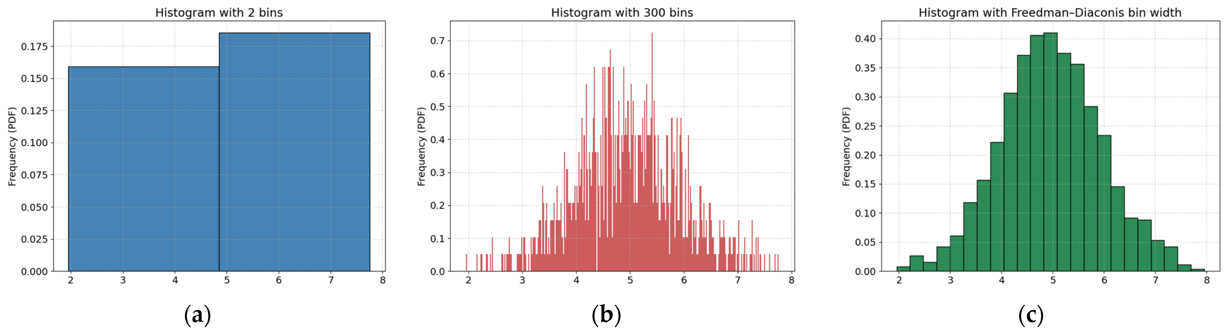
The set of outcomes is post-processed either (i) by assuming an analytic distribution and computing its parameters (for normal distribution that would be mean value μ and standard deviation σ), or, more generally, (ii) by building a histogram. The choice of histogram bin width governs the trade-off between bias and noise in the results—the Freedman–Diaconis rule [33] is a common rule that proposes adequate width.

Figure 1 contrasts two extreme binnings of a synthetic data set—one with very few wide bins and one with many narrow bins—alongside the histogram obtained with the Freedman–Diaconis bin width used in this study. The coarse-bin example shows how excessive smoothing can hide tail behavior and bias density estimates, while the over-refined example reveals the high random variability that arises when too little data fall into each bin. The Freedman–Diaconis (FD) width provides a balance: it is wide enough to suppress random noise yet narrow enough to preserve the essential shape of the distribution. Applying the same rule to our Monte Carlo output yields a stable PDF and ensures that subsequent uncertainty metrics are not artefacts of arbitrary bin selection.

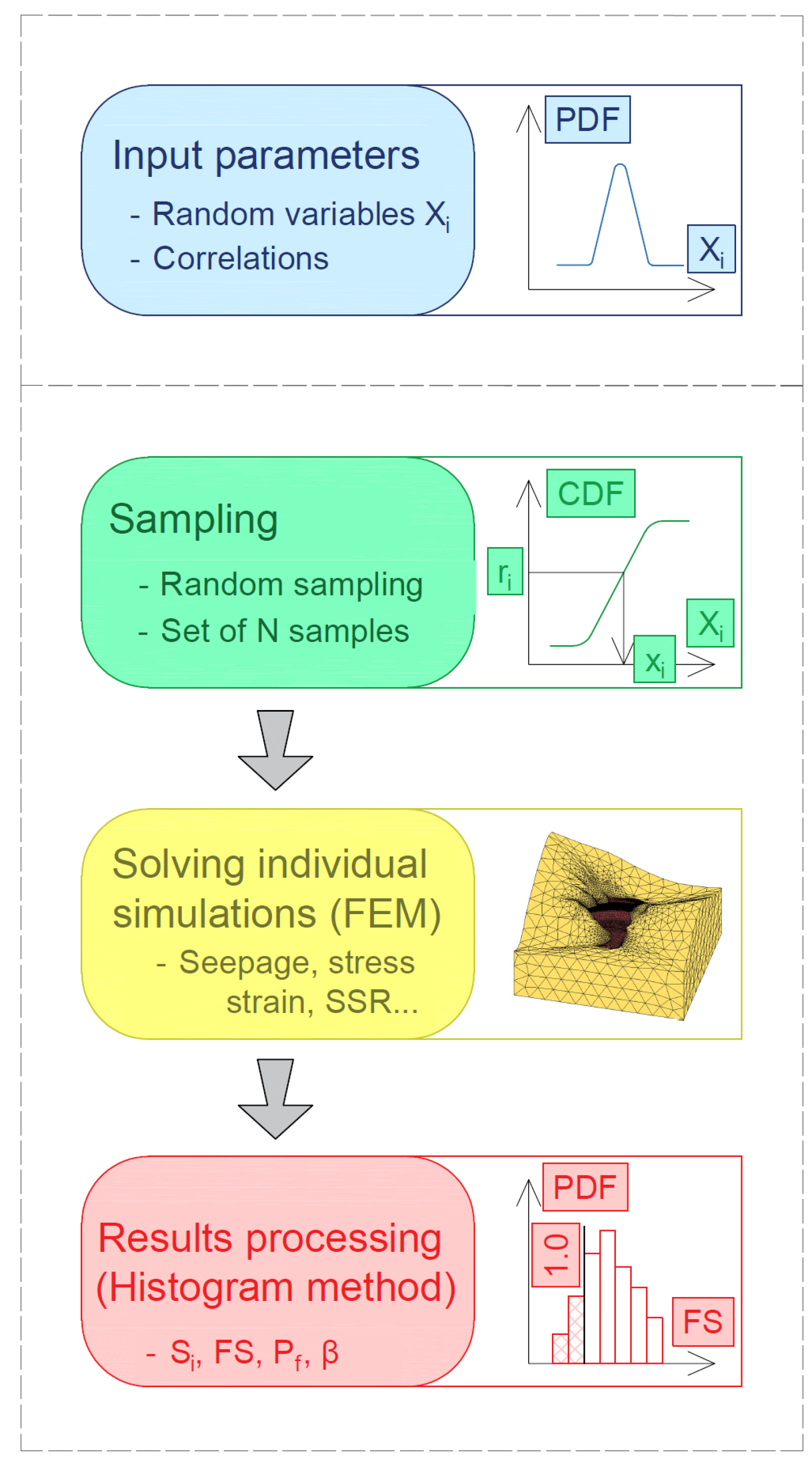
In the present study, a Monte Carlo analysis that uses the histogram method for post-processing constitutes the baseline probabilistic framework which is used as a reference for the proposed monitoring–weighted analysis concept. The flowchart for the baseline Monte Carlo analysis is shown in Figure 2.

The numerical stability of the analysis is verified through convergence plots of the resulting distribution parameters (μ and σ for normal distribution) versus N. If the change in results is negligible after increasing the number of simulations, it is considered that the convergence has been achieved.

3. Methodology Concept

This section introduces a methodology for integrating monitoring data directly into a Monte Carlo probabilistic safety assessment procedure. The key idea is to embed the monitoring data inside a Monte Carlo framework (Figure 2) by weighting each individual simulation according to how closely its predicted behavior matches the monitoring data. Simulations that are closer to the real structural behavior receive higher statistical weight, while those that deviate are suppressed. In effect, the distribution of the baseline Monte Carlo analysis results is “pulled” toward the measured behavior without any need to recalibrate the input parameters themselves. The idea is rooted in Bayesian probability theory [34]: in essence, information from monitoring records updates prior beliefs about system behavior. Although the procedure does not strictly follow a full Bayesian update—no explicit posterior parameter distributions are computed—the weighting step acts as an implicit Bayesian correction, markedly reducing uncertainty and yielding more trustworthy reliability estimates for embankment dams.

The variability of monitoring data must be modeled with care. Only validated, high-quality monitoring readings should enter the update. Any irregular data that misrepresent the structure’s behavior must be removed. Introducing such values into the analysis not only fails to improve the solution’s accuracy, but can produce results that either lie outside the baseline analysis range and prevent convergence entirely or yield overly broad distributions that render the computation uninformative.

It must be pointed out that the dam monitoring data is usually obtained under the operating conditions (far from the failure state). Therefore, analyses scenarios for which monitoring data are used must mirror the actual operating conditions in terms of both the loading history and hydraulic boundary conditions. If extreme design scenarios (such as the safety-evaluation earthquake) have not occurred during the dam’s life, monitoring records cannot validate them directly.

3.1. Mathematical Framework

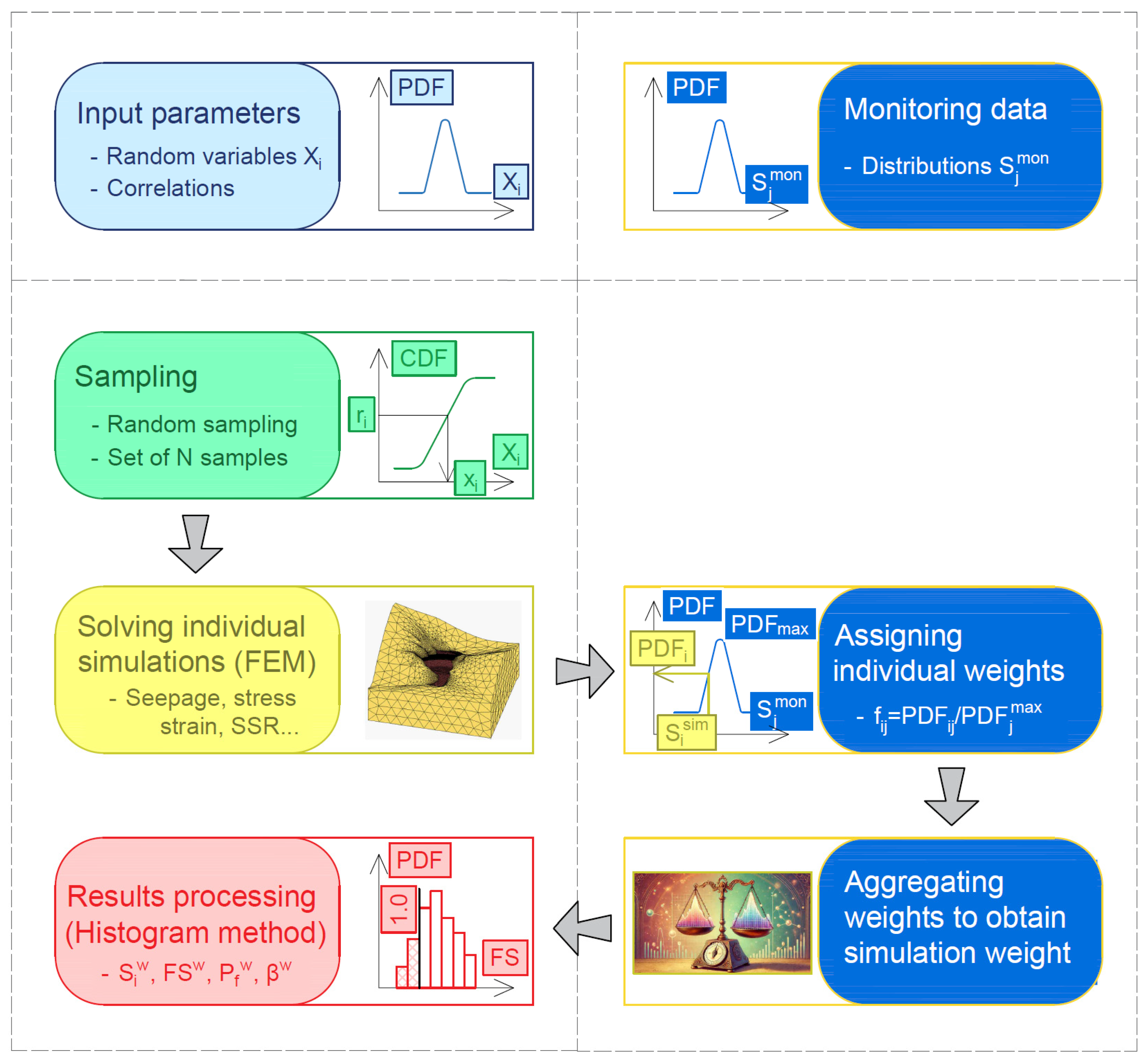
The distributions of monitoring data are denoted as ${S_j}^{mon}$, where $j=1, 2\dots n^{mon}$ represents individual measured quantities, with a total of $n^{mon}$. These distributions must be statistically defined and modeled before the calculation starts, as they represent input data for the probabilistic analysis, which can be referred to as a “weighted” probabilistic analysis. Modeling of the distribution functions of the monitoring data is also performed via a statistical analysis of the available measured quantities. The “weighted” analysis begins in the same way as the baseline analysis, with the sampling of input variables (N sampled combinations) for the computational model. Then, for each parameter combination, the FEM calculation is conducted.

After the calculation, results in each simulation are verified against corresponding monitoring data probability distributions. In this context, the calculation results $S_{ij}$ are being weighted (i = 1, 2, …, N represents a single simulation, and $j=1, 2\dots n^{mon}$ represents one of the results that have a monitoring data distribution). Results that better match the monitoring data ${S_j}^{mon}$ are given a higher impact by introducing weight coefficients $f_i$ for each simulation i. The coefficient $f_i$ is obtained by aggregating the individual weight coefficients $f_{ij}$, which correspond to individual expected distributions of monitoring data.

The procedure for calculating the individual weight coefficients $f_{ij}$ is described as follows:

• Once each FEM run is finished, the relevant response values $S_{ij}$—those matched by available monitoring data—are logged for every simulation i.
• Each result $S_{ij}$ is subsequently evaluated in the monitoring distribution ${S_j}^{mon}$ yielding a probability density ${PDF}_{ij}$, that quantifies how likely that simulation outcome is relative to the observed data.
• The individual weight coefficients $f_{ij}$ for each monitoring data distribution ${S_j}^{mon}$ are calculated as the ratio of the probability density of the simulation result ${PDF}_{ij}$ to the maximum probability density of the function ${S_j}^{mon}$, which is denoted as ${PDF}_{j,max}$:

$$f_{ij}={\displaystyle \frac{{PDF}_{ij}}{{PDF}_{j,max} }}·I_j^w$$

(2)

where the coefficient $I_j^w$ represents the importance weight of each expected distribution ${S_j}^{mon}$ (between 0 and 1). If all results have the same importance, $I_j^w=1$ is adopted for all values of j.

The total weight coefficient $f_i$ (which refers to simulation i) is obtained using the individual weight coefficients $f_{ij}$ by utilizing the chosen aggregation function [35]. The choice of method for combining individual weight coefficients depends on various factors that characterize the specific analysis, such as the complexity and cost of the FEM analysis, the number of monitoring individual distributions and the assigned importance coefficients. In this paper, the product of weights method, given by Equation (3), is chosen as an example. This method calculates the product of the individual weight coefficients within a single observed simulation.

$$f_i={\prod }_{j=1}^{n^{mon}}{f}_{ij}$$

(3)

Next, the histogram of the calculation results is created by considering the weight coefficients of the simulations $f_i$. The frequency of results ${F_k}^{weighted}$ for the observed bin k in the case of a weighted histogram is equal to the sum of the weight coefficients of those simulations whose solutions fall within the range of the bin, that is:

$${F_k}^{weighted}=\sum _{i=1}^{n_k}{f}_i$$

(4)

where $n_k$ represents the number of simulations whose solutions fall within the range of the bin. Weighted histograms take into account the weight coefficient of each simulation when calculating the frequency, which allows for a more accurate estimation of the probability density when the data vary significantly.

The probability density function $PDF\left(x_k\right)$ for the point $x_k$, located at the center of the observed bin k with the bin width h, is equal to:

$$PDF\left(x_k\right)\approx {\displaystyle \frac{1}{N^{weighted}h}}{F_k}^{weighted}={\displaystyle \frac{\sum _{i=1}^{n_k}{f}_i}{h·\sum _{i=1}^N{f}_i}}$$

(5)

where $N^{weighted}=\sum _{i=1}^N{f}_i$ represents the total sum of all weight coefficients.

After the histogram incorporating the weight coefficients is built, all descriptive statistics of the weighted dataset—mode, mean, variance, standard deviation and others—can be readily computed. Figure 3 illustrates the flowchart for performing the weighted probabilistic safety assessment that incorporates monitoring data into the Monte Carlo analysis.

3.2. Scope and Applicability

This section presents the observations and limitations related to the application of the proposed methodology. In Bayesian terms, the baseline Monte Carlo analysis constitutes the prior predictive portrait of dam behavior, summarizing everything believed plausible before new monitoring readings arrive. Monitoring data then enter as the likelihood the statistical measure of how strongly each simulated outcome agrees with the evidence actually captured in the field. The applicability and effectiveness of the proposed methodology is influenced by the relationship between the baseline analysis results (prior) and corresponding monitoring distributions (likelihood). Both the shape and range of these distributions influence the results of the weighted analysis (posterior) which is illustrated in Figure 4 and Figure 5. Moreover, since each simulation’s weight is taking a value between 0 and 1, the effective number of weighted simulations can never exceed the original sample size.

Figure 4 illustrates how the uniformly distributed baseline analysis results are transformed by weighting when the monitoring data follow, respectively, a uniform and a normal distribution. In both cases, the weighted histogram fills the entire overlapping range. Because the monitoring uncertainty covers exactly one-third of the baseline range, precisely one-third of the simulations are retained, and the weighted outcomes match the monitoring data distributions exactly. However, the individual weights are all equal to one for the uniform monitoring distribution, unlike for the normal where far fewer simulations “survive” the weighting unscaled.

Figure 5 depicts how weighting reshapes normally distributed baseline analysis results when the monitoring data are uniform and normal. If the monitoring distribution is uniform (Figure 5a), all simulation weights are equal to one, but only the tail of the normal baseline overlaps the monitoring range, so the weighted histogram consists of that portion of baseline analysis outcomes. When both the baseline and monitoring distributions are normal (Figure 5b), the weighted analysis results are confined to the region where the two normal distributions intersect, yielding a very small weighted simulation count.

Finally, for the weighting to yield meaningful results, the monitoring data distribution must overlap the baseline analysis results’ distribution (i.e., have non-zero probability in its domain). If the observed data lie entirely outside the prior range, the weighting produces zero for all simulation weights and the weighted analysis fails to converge.

Hence, the leverage of the proposed methodology lies in a healthy intersection of the two distributions: the prior must be broad enough to anticipate the range of monitoring outcomes, yet not so diffuse that the corrective influence of monitoring data is drowned in noise. Careful design of the baseline input parameter space and mindful examination of monitoring data and its uncertainty are therefore essential—otherwise, the proposed quasi-Bayesian update degenerates into either an uninformative repetition of the prior or an unstable posterior built on too few retained simulations.

4. Case Study—Safety Assessment of the Rockfill Specimen in Triaxial Test

4.1. Problem Description

Due to the simple and fully controlled boundary conditions, the triaxial test provides a suitable example for demonstrating the presented methodology. The core idea is to treat the triaxial test specimen as an analogue of the real structure whose safety is under investigation; thus, the complex three-dimensional stress distribution within a real structure (e.g., an embankment dam) is reduced to a single, fully controlled stress path that is easy to track and interpret. It should be noted that the real dams may exhibit complex interactions that cannot be captured by this analogy.

The aim is to assess the safety of the reference specimen subjected to a consolidated-drained (CD) triaxial test under the assumption that the test is interrupted at the chosen moment before the material specimen reaches its peak strength (in order to simulate the real structure’s operating conditions). The stress–strain behavior of the specimen is known (monitored) up to this moment and provides the basis for incorporating monitoring data into the probabilistic analysis.

The safety of the reference specimen is evaluated through a Monte Carlo analysis on a FEM model that reproduces the reference specimen test. In each simulation, the factor of safety (FS) is computed using the shear-strength-reduction (SSR) method once the simulated test loading sequence is complete.

Model material parameters are calibrated from the preliminary investigation, using a series of twelve independent triaxial tests. These tests were carried out at different confining stress levels because the eventual confinement for the reference specimen is unknown. The variability observed in the test results is used to define the statistical distributions of the input parameters for the MCS.

Within this compact yet representative example, the reference specimen’s safety at the stoppage point is assessed using two probabilistic approaches for comparison:

• Baseline probabilistic analysis: FS distribution based on nominal (prior) distributions of the input parameters.
• Weighted probabilistic analysis: FS distribution based on the baseline distributions adjusted in accordance with the available monitoring data (posterior).

4.2. Preliminary Investigation

The twelve triaxial tests used in this study to calibrate material parameters for the safety assessment of the reference specimen form part of a broader laboratory campaign on embankment materials undertaken for the ongoing dam project in Asia. All tests are carried out in the ISMGEO laboratory in Bergamo, Italy. The examined material is the rockfill that constitutes the dam slopes and protects the central clay core. The tests are run with four different values of confining cell pressure σ′₃: 250 kPa, 500 kPa, 1000 kPa and 2000 kPa (three samples for each σ′₃).

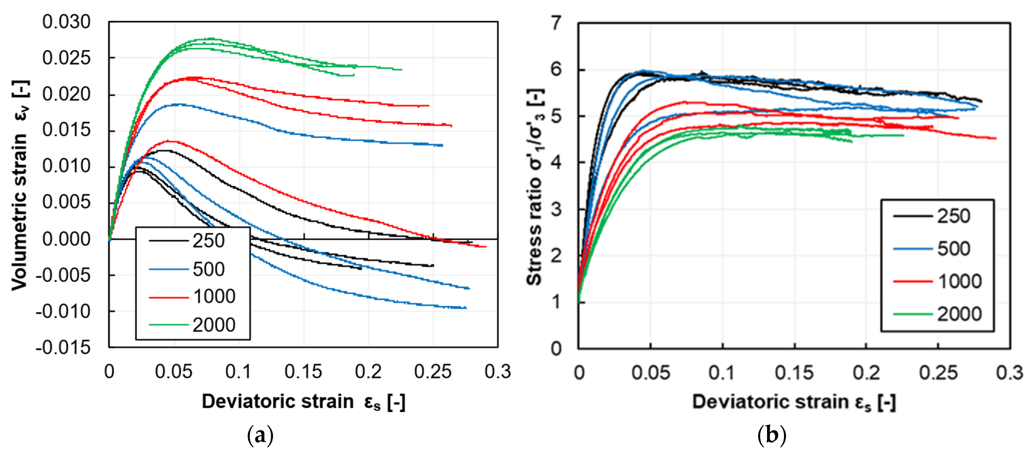
The deviatoric behavior observed in triaxial compression is presented in Figure 6. All specimens exhibit non-linear strain hardening from very small strains up to the peak strength. After the peak, the specimens tested at lower confining pressures show a slight tendency to soften.

The volumetric contraction occurs up to approximately the peak strength; after that, the material behavior becomes dilative, as shown in Figure 7. Samples tested at the lower confining pressures display more tendency for dilatancy. Although testing continues to ε_s ≈ 25%, not all specimens reach a constant-volume state.

Figure 7 also plots the stress ratio σ′₁/σ′₃ against the deviatoric strain, giving a clearer visual basis for comparing peak and constant-volume (CV) states. The difference between peak and CV stress ratios is clear at σ′₃ = 250 kPa and diminishes as the confining pressure rises, becoming almost imperceptible at σ′₃ = 2000 kPa.

The four test groups reveal how the material responds at different confinement levels. Key stress–strain characteristics—strength, stiffness and dilatancy—vary with σ′₃ as follows:

• Strength rises non-linearly with confining pressure; the σ′₁/σ′₃ ratio at failure decreases as σ′₃ increases (Figure 7).
• Stiffness increases with the higher confinement level (Figure 6).
• Dilatancy becomes less pronounced at higher stresses and is almost negligible for σ′₃ = 2000 kPa (Figure 7).

4.3. Monitoring Data

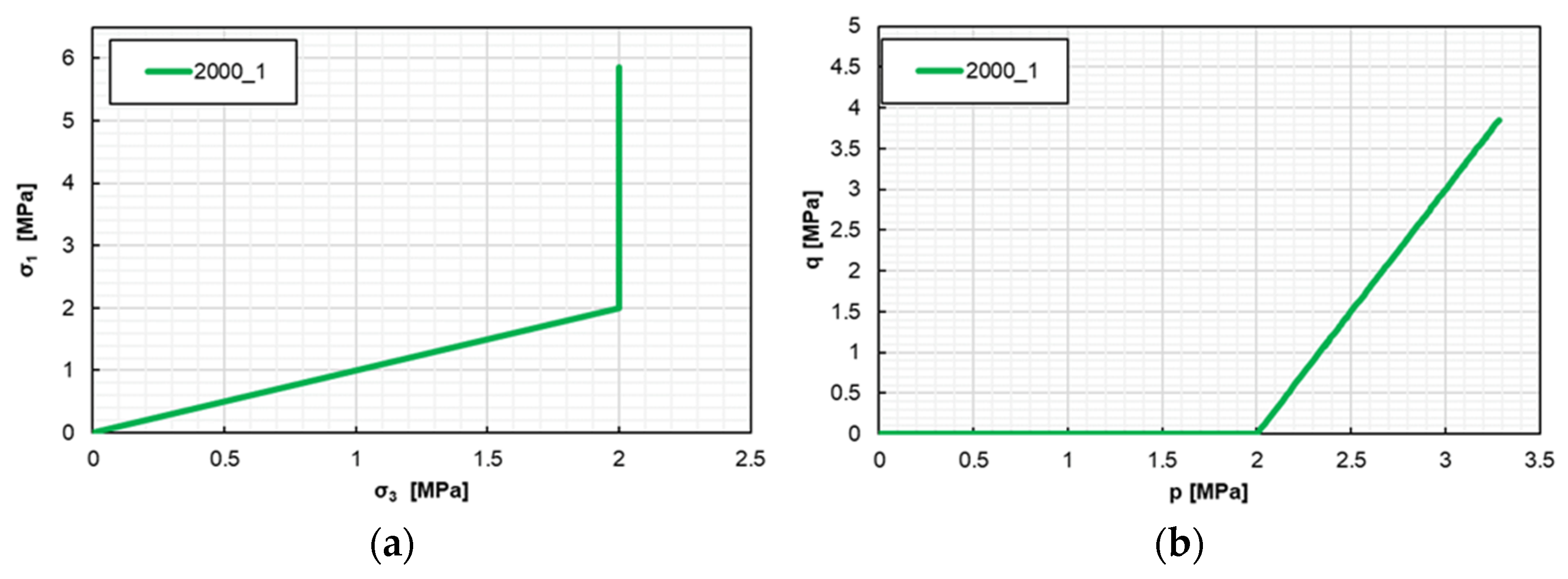
The monitoring data incorporated in this example correspond precisely to the stress–strain state of the reference specimen captured at the moment the triaxial test is halted, before the material reaches its peak strength. At the selected stopping point in the shearing phase, the confining stress is σ′₃ = 2000 kPa, while the axial stress has increased to σ′₁ ≈ 5860 kPa (Figure 8). At this point, the safety of the specimen is assessed. Before stopping the test, the specimen behaves as shown in Figure 9, with a final observed axial strain ε₁ = 2.45%.

The defined analysis scenario places the reference specimen in the high-confinement domain (σ′₃ = 2000 kPa), which is a random event and could not be anticipated when the investigation testing campaign was set for a broad range of possible stress states. Material parameters calibrated from the 12 test results cannot easily reproduce the actual response in one specific portion of the pre-defined broader range. Hence, in this scenario, the monitoring data play a crucial role: they steer the baseline safety analysis, which spans a broader spectrum of possible behaviors, toward the zone that reflects the actual material response.

4.4. Numerical Modeling

The safety assessment of the reference specimen is evaluated probabilistically by running a Monte Carlo analysis on a dedicated FEM model. Model inputs include material parameters and boundary conditions. While material parameters are considered as random variables, the boundary conditions are defined in the same way for each Monte Carlo simulation since they describe the monitored test conditions described in the previous chapter.

4.4.1. FEM Model Setup

The cylindrical triaxial reference specimen is idealized with an axisymmetric two-dimensional FEM model using Rocscience software RS2 [36], exploiting the specimen’s rotational symmetry and the symmetry of the loading conditions. Only one half of the sample is discretized: a square domain of the unit height and unit radius is meshed with one eight-noded quadratic element [37]. The symmetry axis is defined along the left-hand vertical boundary, where radial displacements are constrained, while the base is fully fixed in the vertical direction to mimic the actual test conditions. Figure 10 illustrates the model geometry and restraints.

The selected constitutive model is linear elastic: a perfectly plastic Mohr–Coulomb model, due to its simplicity, intuitive interpretation and wide practical use, especially in stability problems. The limitations of the Mohr–Coulomb model with respect to the actual material behavior are as follows: constant stiffness for different confining stress levels, constant dilation angle at different stress levels as well as a linear failure envelope.

The triaxial test loading procedure is reproduced in two sequential phases (Figure 11). During the isotropic compression phase, the model is subjected to equal radial and axial stresses, i.e., σ′₁ = σ′₂ = σ′₃ = 2000 kPa, applied as uniform pressure boundary conditions on the lateral and upper free surfaces. In the subsequent shearing phase of the test, confining (radial) stress σ′₂ = σ′₃ = 2000 kPa is held constant, whereas the axial stress is increased to the value σ′₁ = 5860 kPa.

Once the triaxial loading phase concludes, the FEM model retains the specimen’s current stress–strain state and exports it into the shear strength reduction (SSR) procedure. The SSR method then evaluates the factor of safety by gradually lowering the shear strength parameters by a trial factor F while keeping the external loads and boundary conditions fixed. The solver attempts to reach equilibrium with such reduced parameters. If the convergence is reached, the specimen is still stable at that strength level; if convergence fails or the incremental displacements increase excessively, it is considered that the failure has occurred at that reduction factor F. By successively increasing F, the analysis arrives at a critical value F_crit at which stability is lost. This value is reported as the factor of safety (FS), and it represents the margin by which the material’s shear strength could be uniformly scaled down before the reference specimen, in its current stress state, would collapse. Because the loading history is fixed and only strength is modified, the SSR procedure provides a consistent safety metric for every Monte Carlo simulation.

4.4.2. Material Parameters’ Calibration

To calibrate the parameters of a Mohr–Coulomb model, each of the twelve triaxial tests from the preliminary investigation is reproduced in the FEM environment using Rocscience software RS2 [36]. The model calibration is conducted under the following assumptions:

• Experimental results point to a non-cohesive material structure—expected for rockfill—so effective cohesion is neglected (c’ = 0). Strength is therefore controlled solely by the effective friction angle φ’.
• The value of φ’ is assigned according to the maximum axial stress σ′₁ attained in the test; any post-peak softening is ignored.
• An elastic modulus equal to the secant modulus E₅₀, measured at 50% of σ′₁^max on the σ′₁–ε₁ curve, is adopted. The secant modulus E₅₀ provides a balanced, single-value approximation of soil stiffness in the majority of the stress path of triaxial loading, especially in the part representing working stress levels (analogy with the real structure safety assessment).
• Poisson’s ratio (ν) and the dilation angle (ψ) are determined by least-squares optimization so that the model reproduces the observed dilatant behavior evident in the volumetric–axial strain curve.

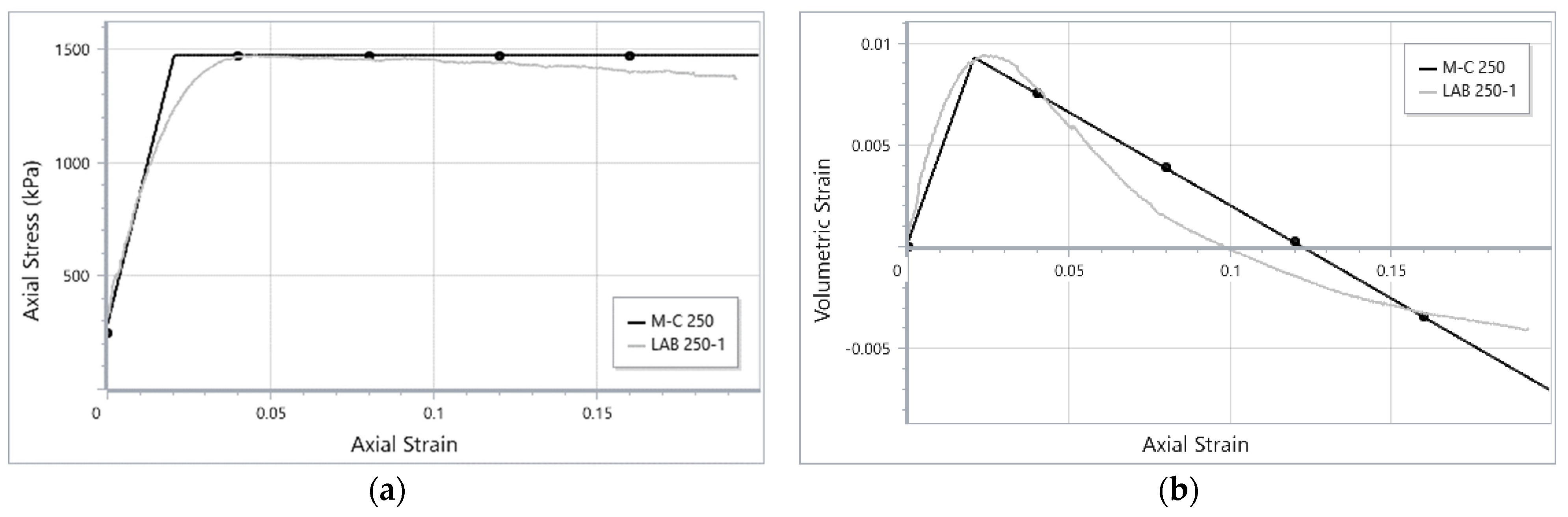
Figure 12 provides an example of the test recreation based on one of the triaxial tests from the preliminary investigation. The calibrated parameters are listed in

Table 1. Calibrated Mohr–Coulomb model parameters from 12 triaxial tests.

Sample No.	σ′3 (kPa)	φ’ (°)	E50 (MPa)	ψ (°)	ν (-)
1	250	45.2	58	2.5	0.28
2		45.4	66	2.3	0.24
3		45.5	48	2.0	0.25
4	500	45.5	105	3.4	0.27
5		45.2	87	2.8	0.30
6		42.6	65	0.9	0.21
7	1000	43.1	125	2.0	0.30
8		42.2	100	1.2	0.22
9		41.2	95	0.8	0.22
10	2000	40.2	155	0.5	0.22
11		40.3	145	0.9	0.22
12		41.0	160	0.8	0.21

. More details on the triaxial test recreation procedure are presented in [38].

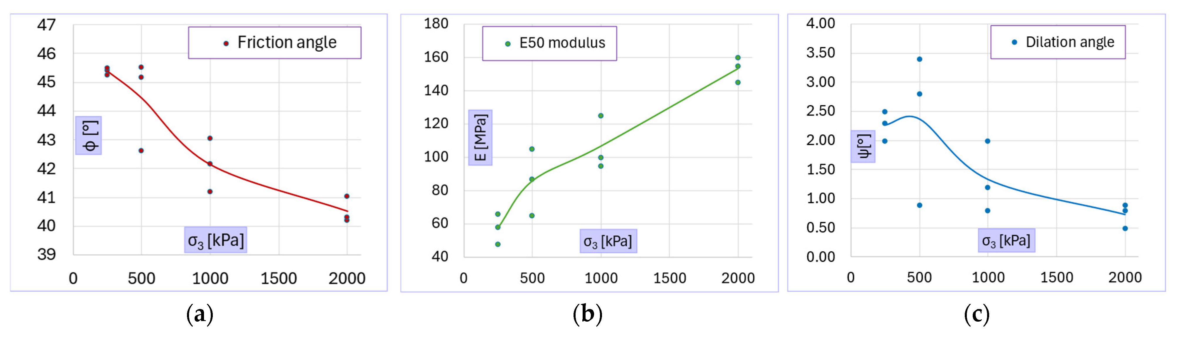
Figure 13 illustrates how the calibrated material parameters change with the confining stress level. In line with the behavior observed during testing, the calibrated parameters indicate a decrease of the effective friction angle (non-linear failure criterion), an increase in stiffness, and a reduction in dilatancy as the confinement level rises. Poisson’s ratio shows no clear dependence on stress level.

4.5. Variability Modeling

4.5.1. Mohr–Coulomb Parameters for FEM Model

The first step of the Monte Carlo analysis consists of modeling the variability of the input parameters, i.e., defining the functions that characterize their statistical distributions. In this case, the effective friction angle φ’ and the elasticity parameters (E, ν) are assumed to follow normal distributions, while the dilation angle ψ follows a gamma distribution (

Table 2. Input variables and parameters of assigned statistical distributions.

Variable	Distribution	Parameters 1
φ’ (°)	Normal	μ = 43.12, σ = 2.15
E (MPa)	Normal	μ = 100.8, σ = 38.54
ψ (°)	Gamma	α = 3.13, β = 0.54
ν (-)	Normal	μ = 0.25, σ = 0.03

¹ μ, σ are the mean and standard deviation of the normal laws; α, β are the shape parameters of the gamma law.

). The parameters of these distributions are derived from the twelve calibrated finite-element reconstructions of the laboratory tests and summarized in Table 2. For variables assumed to follow a normal distribution (φ’, E, ν), the mean and standard deviation are computed directly from the calibrated parameters’ dataset (Table 1). For the variable ψ modeled with a gamma distribution, the shape (α) and scale (β) parameters are calculated using the standard moment-based relations: α = ²/σ² and β = σ²/μ, where μ and σ represent the sample mean and standard deviation, respectively.

The trends displayed in Figure 13 imply that the key material parameters are not statistically independent, but exhibit systematic interrelations that must be preserved in any probabilistic assessment:

• Effective friction angle (φ’) vs. stiffness (E): As confinement increases, φ’ falls while E rises, yielding a pronounced negative correlation. Specimens with a lower elastic modulus consistently mobilize higher peak friction, whereas highly confined (and therefore stiffer) specimens mobilize a reduced φ’.
• Effective friction angle (φ’) vs. dilation angle (ψ): Both angles diminish with increasing confinement, resulting in a clear positive correlation where larger friction angles are accompanied by larger dilation angles, and vice versa.
• Stiffness (E) vs. dilation angle (ψ): Because E rises and ψ falls with confinement, these variables are negatively correlated.

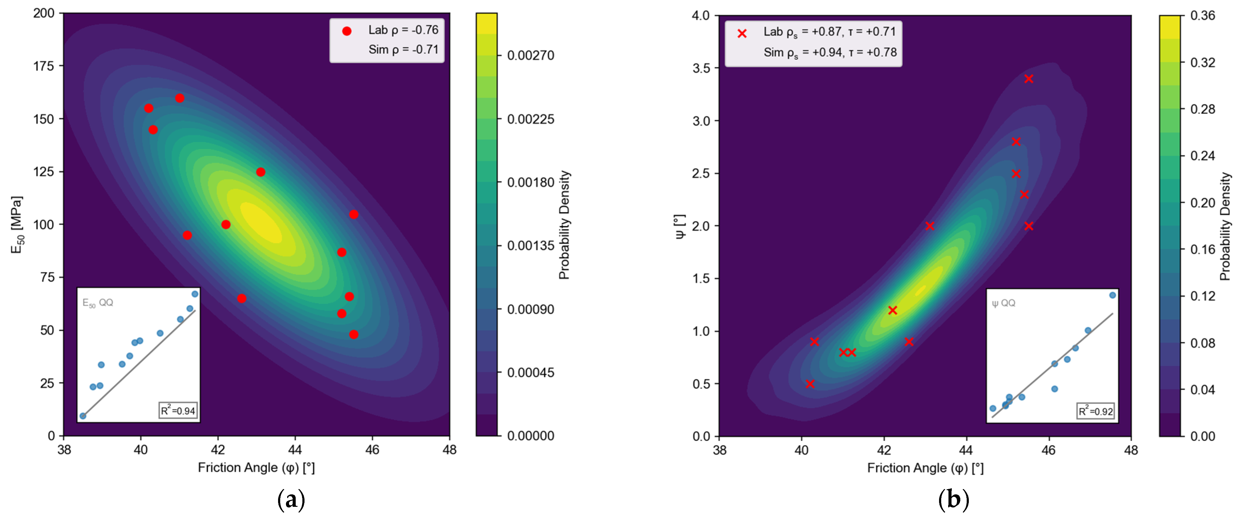
These couplings are captured by (i) a bivariate normal distribution for the φ’–E pair, and (ii) a Gaussian copula linking φ’ and ψ, which subsequently induces the appropriate secondary dependence between E and ψ. The correlation structure is introduced in the following way:

• φ’–E pair: A bivariate normal distribution is defined with a Pearson correlation coefficient [39] calculated from the laboratory data (Pearson ρ = −0.76).
• φ’–ψ pair: A Gaussian copula [40] links the variables in the following manner: φ’ is mapped to a uniform variate via its normal cumulative distribution, which is then transformed to ψ through the inverse gamma CDF (Spearman ρ_s = 0.87, Kendall τ = 0.71).

Introducing the parameters in this correlated form ensures that the Monte Carlo sampling considers the physically observed tendencies and yields a realistic spread of input combinations for the safety analysis (Figure 14). A 10,000-sample Monte Carlo set preserves the laboratory-obtained correlation metrics within close range (ρ = −0.71; ρ_s = 0.94; τ = 0.78). Quantile–quantile (QQ) diagnostics in Figure 14 confirm that both marginal fits and joint tails are adequately reproduced (all points stay close to the 45° line, R² > 0.9).

4.5.2. Monitoring Data

To embed the reference specimen monitoring records in the probabilistic framework, and be consistent with the proposed methodology formulation, the axial strain is treated as a synthetic, normally distributed variable rather than as a single fixed value, with a mean μ =2.45% and standard deviation σ = 0.002. The chosen—small but non-zero—standard deviation keeps the monitoring data distribution tightly centered on the actual measurement, while avoiding the numerical instability that a perfectly deterministic (σ = 0) “spike” would cause later, when weights are assigned. A stricter quasi-deterministic choice such as σ = 0.0002 would require about 10⁶ simulations to reach convergence, while σ = 0.002 leads to 10,000 simulations.

4.6. Probability Analysis Results

The Monte Carlo analysis—10,000 simulations of the triaxial test FE model—is carried out with the full correlation structure observed in the laboratory data (negative φ’–E and positive φ’–ψ links). Ten thousand input quadruples (φ’, E, ψ, ν) are generated using a Python script. These samples provide the stochastic basis for the subsequent Monte Carlo safety assessment. Histogram bin widths are selected with the FD rule and tested ±50% around that optimum bin width value. The resulting change in the estimated mean and standard deviation of obtained distributions is less than 0.3%, demonstrating that the bias–variance trade-off is negligible at the 10,000 sample size.

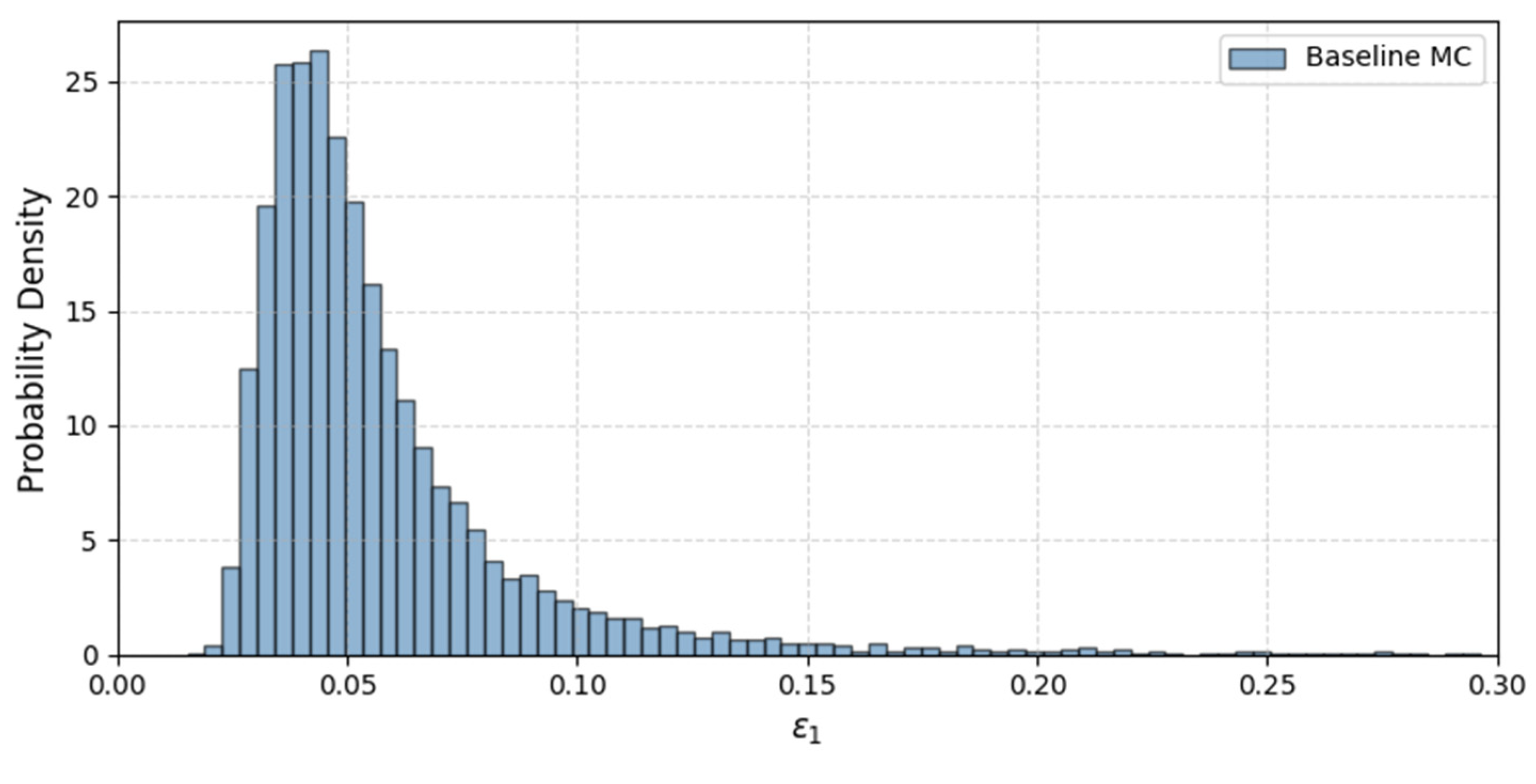
Figure 15 shows the baseline probability density function (PDF) of calculated axial strain ε₁ from the baseline Monte Carlo simulations. Most simulated strains lie below 0.20, although a small number exceed 0.25 owing to samples with very low elastic modulus E.

Figure 16 compares the ε₁ PDFs before and after weighting. For clarity, the plot trims the baseline curve at ε₁ > 0.10; the long right-hand tail (up to ε₁ ≈ 0.30) remains in the data set but is visually uninformative. After weighting, the ε₁ distribution localizes around the monitored value, demonstrating that the procedure pulls the simulation ensemble toward the observed behavior, which is confirmed by a very high Kullback–Leibler (KL) divergence [41] (≈2.9 nats) between baseline and weighted PDFs.

Regarding the factor of safety according to SSR, a baseline analysis yields the FS distribution with a mean μ = 1.69 and standard deviation σ = 0.11 (Figure 17). Introducing the monitoring data–normal distribution centered on the measured axial strain (ε₁ = 2.45%, σ = 0.002) and weighting each simulation accordingly shift the outcome markedly (KL divergence is registered ≈1.6 nats): the mean FS drops to μ = 1.48 and the spread narrows to σ = 0.08. The decrease in the mean value of FS from 1.7 in baseline to 1.5 in weighted analysis reflects that the lower friction angle is generally mobilized at the higher confinement level.

Although the baseline run comprises 10⁴ simulations, the weighting step reduces the weighted simulation count to only about 235 and effective sample size (ESS) [42] to ≈372 (Figure 17). The resulting histogram is therefore noticeably rougher than the baseline version.

5. Discussion

5.1. Convergence Observations—Number of Simulations

To determine how many simulations are required for numerical stability, the convergence of the mean and standard deviation of FS are examined for both baseline and weighted analyses. They are evaluated by performing 100 additional complete Monte Carlo analyses with logarithmically spaced sample sizes from 1 to 10⁶ and plotting μ and σ versus simulation count. Additionally, the KL (FS) convergence curve is created within the same numerical procedure.

Figure 18 displays the convergence curves for the mean and standard deviation of FS distribution. It indicates that 10,000 simulations are optimal: beyond this, μ and σ of the weighted analysis histogram no longer change appreciably. The baseline and weighted analysis do not converge with the same number of simulations. The computational cost of the weighted analysis depends on the effective subset of the nominal number of simulations that retain non-negligible weight after the monitoring data filter has been applied. This is referred to as the weighted simulation count (sum of all weights) $N^{weighted}$.

Figure 18 shows that the baseline Monte Carlo results stabilize with roughly 300 simulations, whereas the weighted analysis attains convergence only when the nominal simulation count is increased to about 10⁴. The disparity arises because, after weighting, those 10⁴ simulations contribute an effective count of just 235 (Figure 17), which is comparable to the 200 simulations that suffice for the unweighted case.

Figure 19 demonstrates that the KL divergence exhibits considerable variability at small sample sizes due to the insufficient population of the weighted histograms. Once the simulation count surpasses approximately 10⁴ simulations, the KL converges to a steady value of approx. 1.6 nats—a plateau that matches the reported KL value in Figure 17. Beyond this threshold, additional simulations yield negligible further change of KL divergence, signifying that the informational content conveyed by the monitoring data has been effectively exhausted.

The weighted simulation count $N^{weighted}$ is presented in Figure 20 against the standard deviation of the monitoring data (σ_mon), for four nominal simulation counts N. Four Monte Carlo sets of samples are created: a barely converging set of 200 simulations and three progressively larger sets of 10³, 10⁴ and 10⁵ samples. For each set, the complete weighted analysis is repeated 100 times while the monitoring standard deviation σ_mon is varied logarithmically from 0.0002 to 0.2 (0.1–99% ε_1,range from baseline MC analysis). For each σ_mon value, the weights are summed up to obtain the $N^{weighted}$. The whole described procedure is then repeated 50 times with different N samples in each of the four sets. This produces 50 values of the $N^{weighted}$ for each σ_mon. Figure 20 plots the mean of those 50 values as the solid curves and shades the regions covering ±2 standard deviations of $N^{weighted}$ distributions. The shaded envelopes therefore visualize the spread of $N^{weighted}$ that arises purely from the random selection of nominal simulations N.

When the monitoring standard deviation is roughly one percent (0.002) or more of the baseline spread, a nominal set of about 10⁴ Monte Carlo simulations already supplies several hundred effective draws, yielding a well-resolved posterior at a modest cost. If the monitoring span tightens to a few-tenths of a percent, however, the effective sample size collapses below the practical threshold of 200, and the posterior becomes noisy unless the nominal simulation count N is expanded by several orders of magnitude. The shaded ±2 σ envelopes indicate visually where the convergence is assured. When the shading remains narrow and entirely above the 200-simulation reference line, the effective sample size $N^{weighted}$ is essentially stable and the weighted analysis is converged. Where the shading widens appreciably (below 200-simulation line), the large dispersion in $N^{weighted}$ denotes practical non-convergence, indicating that a larger nominal simulation count N or a less restrictive σ_mon is necessary.

5.2. Influence of the Monitoring Data Span on Axial Strain ε₁ and Factor of Safety FS

In the weighted analysis, the measured axial strain (ε₁ = 2.45%) is represented by a normal distribution. Its standard deviation (σ) controls how strictly the weighting procedure steers the Monte Carlo analysis toward the monitored value. To quantify this effect, four different spans of axial strain distribution are examined, and a probabilistic analysis is rerun with N = 10⁶ simulations to ensure convergence even for very small (quasi-deterministic analysis) standard deviations (

Table 3. Monitoring data span definitions. The chosen ε_1,range is ~0.20, according to baseline MC results (Figure 15).

Monitoring Data	σ/ε1,range	σ (Absolute)	Qualitative Description
Quasi-det	0.1%	0.0002	quasi-deterministic
Tight	1%	0.002	narrow
Wide	10%	0.02	moderate
Very wide	100%	0.2	full baseline range

).

The probability–density curves in Figure 21 illustrate how the choice of monitoring-data span (σ) governs the influence of the weighting procedure:

• Quasi-deterministic span: The PDF collapses almost into a spike at ε₁ = 2.45%. Only a handful of simulations retain appreciable weight, confirming that an extremely narrow span drives the analysis toward a virtually deterministic match with the observation (extremely high KL = 5.4 nats confirms this), but at the cost of a very large number of simulations necessary to secure convergence.
• Tight span: The distribution remains centered reasonably close to the measured strain (KL = 2.9 nats still indicates a very strong pull), yet preserves a finite (small, but not negligible) spread. This span still filters out more than 98% of the baseline tail, providing a strong monitoring pull while needing only around 10⁴ simulations for reliable statistics.
• Wide span: The peak shifts only modestly toward the monitoring (KL = 0.3 nats); a residual right-hand tail survives. The monitoring data influence the results, but the baseline variability is far from eliminated.
• Very-wide span: The weighted curve is virtually indistinguishable from the baseline histogram (KL ≈ 0 indicates negligible information gain), demonstrating that an observation span comparable to the full baseline scatter leaves the analysis effectively unweighted.

Figure 21. Axial-strain ε₁ probability densities: baseline analysis versus weighted analyses with different monitoring spans. KL divergence values are presented in the legend.

Figure 21. Axial-strain ε₁ probability densities: baseline analysis versus weighted analyses with different monitoring spans. KL divergence values are presented in the legend.

Figure 22 mirrors the span trend for axial strain but now in terms of the factor of safety distributions.

As the monitoring data standard deviation contracts from “very-wide” to “quasi-deterministic”, the entire probability-density function of the factor of safety (FS) shifts leftward and tightens:

• Quasi-deterministic span: the green PDF peaks at μ ≈ 1.45 with the smallest spread, representing the strongest monitoring pull (KL = 1.99 nats) but achievable only with around a million-simulation analysis.
• Tight span: the red curve moves decisively (KL = 1.56 nats) into the lower FS regime (μ ≈ 1.48) and its variance drops by roughly one quarter; the results now reflect the lower effective friction angle mobilized at high confinement.
• Wide span: the purple curve shows a modest left shift (μ ≈ 1.62) and a slight narrowing; monitoring data begin to influence the FS estimate but the baseline analysis variability still dominates (confirmed by low KL = 0.13 nats).
• Very-wide span: the orange curve is practically indistinguishable from the blue baseline (KL ≈ 0); weighting is neutral when the monitoring span covers the full baseline analysis range.

Table 4. Effects of monitoring data span on FS statistical measures.

σ/ε1,range	μ (FS)	σ (FS)	KL (FS)
0.1%	1.45	0.06	1.99
1%	1.48	0.08	1.56
10%	1.62	0.10	0.13
100%	1.69	0.11	0

presents the effect of the monitoring data range on the FS statistics.

A narrow monitoring PDF distribution span lowers the estimated safety level (by up to 14% relative to the baseline μ = 1.69) and tightens its dispersion; these results reflect the variability of the (lower) effective friction angle mobilized at the high confinement. As the span widens, the results eventually revert to the baseline values.

Combined with the ε₁ results (Figure 21), it is confirmed that a 1% span offers the best compromise: it meaningfully updates the safety prediction (KL divergence is high for both ε₁ and FS), trims the variance and remains computationally tractable with 10⁴ simulations.

6. Conclusions

An original methodology for integrating the stochastic monitoring data into the Monte Carlo probabilistic safety assessment procedure without recalibrating the input parameters’ distributions has been presented. The concept of “weighted” simulations according to how closely they match the monitoring data has been introduced.

The described methodology was tested on a case study of CD triaxial testing of the rockfill material, with the idea that the triaxial test specimen mimics the real structure, whose safety is under investigation. Input variables for the baseline probabilistic analysis were based on material parameters calibrated from recreated laboratory tests in the FEM environment using the Mohr–Coulomb material model.

Based on the presented methodology and case study, the following conclusions can be made:

• Incorporating monitoring data systematically shifts results toward the behavior actually observed in the field and narrows their scatter. For the triaxial-test specimen, the mean factor of safety (FS) dropped from 1.69 to 1.48 and its standard deviation fell by roughly one-quarter after weighting, revealing a more conservative—and better defined—safety estimate.
• A meaningful overlap between baseline and monitoring distributions is essential. If the observed data lie completely outside the prior envelope, all weights collapse to zero and the analysis cannot converge; conversely, if monitoring uncertainty spans the entire prior envelope, the update is uninformative.
• The tighter the monitoring distribution, the stronger (and more localized) the update, but the larger the baseline sample required for convergence. Quasi-deterministic monitoring in the case study (σ ≈ 0.1% of baseline range) obtained best results but demanded the order of 10⁶ baseline simulations.
• Practical success depends on aligning monitoring uncertainty with prior variability. If the monitoring range is overly narrow, too few simulations receive meaningful weight and convergence falters; if it is excessively wide, the weights become nearly uniform, and the update adds little new information. The case study demonstrated this statement.
• Preserving correlations among input parameters is critical; otherwise, the weighting step may keep and even exaggerate physically impossible combinations. In the case study, embedding the negative φ′–E and positive φ′–ψ correlations ensured realistic parameter combinations and prevented uninformative weighting.
• The procedure remains computationally tractable for routine problems. With a monitoring standard deviation equal to ~1% of the baseline spread in the case study, 10,000 baseline simulations yielded ~200 effectively weighted simulations; these are sufficient for smooth posterior histograms and stable statistics.

The presented methodology offers a transparent and computationally tractable route for embedding monitoring data into routine engineering calculations, thus producing more realistic safety estimates of actual structural behavior. Although this methodology is developed in the context of embankment dam safety, it can be applied to other structural systems where systematic long-term monitoring is implemented. It must be pointed out that the structural monitoring data usually reflect the operating conditions (far from the failure state); therefore, analyses must mirror the actual operating conditions. If extreme design scenarios have not occurred during the observed period, monitoring records cannot validate them directly. However, there is potential to extend the proposed methodology to imaginary or extreme scenarios not yet observed during the dam’s service life, possibly using conditional modeling or extrapolation techniques. The presented investigation can lead to further research topics, as follows:

• The product of weights method presented in this study for calculating the overall simulation weight coefficient provides a decent option, especially if it is possible to execute a sufficiently large number of FEM simulations. However, other similar methods should be benchmarked as well, especially if they can lead to a smaller number of simulations.
• In problems where further statistical efficiency is required, two additional techniques are recommended: (i) parametric bootstrapping of the weighted sample, which tightens confidence intervals without additional FEM runs; and (ii) importance sampling aimed at the high-weight region.
• The estimation of the required simulation count given the desired precision of the weighted analysis should be further investigated.
• The presented methodology should be demonstrated in the case study of a real and more complex structure, such as an embankment dam.