Research on the SSUKF Integrated Navigation Algorithm Based on Adaptive Factors

Abstract

In complex environments, the application of traditional Kalman Filtering in GNSS/INS integrated navigation systems often encounters challenges such as filter divergence and accuracy degradation. This paper introduces the technique of Simplified Spherical Unscented Kalman Filtering (SSUKF) and, based on this, proposes an Adaptive Simplified Spherical Unscented Kalman Filtering (ASSUKF) integrated navigation method. This approach, built upon SSUKF, incorporates an adaptive filter that effectively utilizes residuals and innovation sequences to mitigate the divergence phenomenon during the filtering process. Furthermore, the system is capable of online estimation and dynamic adjustment of the statistical characteristics of measurement noise, leading to more accurate state estimation and significantly enhancing the adaptive capability of SSUKF. ASSUKF improves position accuracy in the latitude direction by 18.10% and in the longitude direction by 20.6%. For attitude error, ASSUKF performs exceptionally well. Specifically, the pitch angle error improves by 27.6% compared to UKF and by 27.1% compared to SSUKF. The roll angle error improves by 29.9% compared to UKF and by 20.1% compared to SSUKF. The heading angle error improves by 24.3% compared to SSUKF, validating the method’s substantial advantages in improving system accuracy and robustness, demonstrating its effectiveness and potential in complex environments.

1. Introduction

The Global Navigation Satellite System (GNSS), as a satellite-based positioning system, is widely applied in fields such as transportation, communications, and scientific research. The GNSS determines an object’s position, velocity, and time by receiving satellite signals, offering precise global positioning services without geographic constraints. It provides stable satellite signals in diverse environments, such as cities, oceans, and remote areas, enabling high-precision positioning [1]. However, despite its capability to provide decimeter-level or higher accuracy in open environments, the GNSS still faces some notable shortcomings and challenges in practical applications. Firstly, GNSS signals are easily affected by obstacles, interference, and multipath effects [2]. Particularly in urban canyons, tunnels, and densely wooded areas, signal transmission becomes unstable, significantly reducing positioning accuracy. In these environments, satellite signal transmission is severely restricted, preventing the system from delivering accurate location information. Furthermore, GNSS positioning accuracy can also degrade under extreme weather conditions.

To address these issues, the inertial navigation system (INS) has emerged as an important complement to the GNSS, serving as an autonomous navigation solution. The INS does not rely on external signals and uses built-in inertial sensors, such as accelerometers and gyroscopes, to measure an object’s acceleration and angular velocity, thereby calculating its position, velocity, and orientation [3]. Since INS operates independently of external signals, it can still provide reliable navigation information in GNSS-denied environments (such as underground, in tunnels, or within buildings). The INS is characterized by its high-frequency response, making it suitable for highly dynamic environments, and it can provide relatively high positioning accuracy over short periods. However, the main drawback of the INS is the accumulation of errors [4]. Over time, drift and noise from the inertial sensors lead to the gradual accumulation of system errors, which affects navigation accuracy. Therefore, relying solely on the INS for positioning results in a decline in accuracy over time, making it difficult to maintain high-precision navigation over extended periods.

To overcome the limitations of both the GNSS and INS, GNSS/INS integrated navigation technology has become a research focus in recent years [5]. By combining these two systems, their respective strengths can be fully utilized, compensating for the shortcomings of each when used independently. Specifically, the GNSS provides high-precision positioning information on a global scale but is limited in certain environmental conditions; the INS, on the other hand, can provide continuous navigation information when the GNSS is unavailable. By integrating the advantages of both, more accurate and stable navigation results can be achieved in complex environments.

In integrated navigation systems, data fusion algorithms play a crucial role. Their primary task is to effectively integrate data from different sensors (such as the GNSS, the INS, and visual sensors) to provide more accurate and reliable navigation information. Common data fusion algorithms include Kalman Filtering [6] (KF), Extended Kalman Filtering [7] (EKF), and Particle Filtering [8] (PF), which optimize the weighted fusion of sensor data to reduce noise effects and allow real-time updates in dynamic environments. However, Kalman Filtering requires precise mathematical models and accurate prior noise statistics, and when noise characteristics deviate from those expected, filtering accuracy may deteriorate or even diverge [9]. To address this issue, researchers have made numerous improvements to the Kalman Filtering algorithm [10]. Since standard Kalman Filtering is only applicable to linear systems and not to nonlinear ones, the Extended Kalman Filter (EKF) was proposed, which linearizes the state transition and observation equations of a nonlinear system using a first- or second-order Taylor expansion [11] for state estimation. Building on this, scholars proposed the Error-State Extended Kalman Filter [12] (ESEKF), which estimates the error in the state vector to reduce the impact of nonlinearity on the system, though this approach can be computationally intensive for high-dimensional systems or complex models.

Unscented Kalman Filtering (UKF) was firstly proposed by Julier and Uhlman in 1997 [13] and has gained widespread attention as a new filtering method in recent years [14]. Unlike EKF, UKF handles nonlinear systems more accurately through the “unscented transformation” rather than linearization. By using unscented transformation, UKF captures higher-order statistical information about the system state, providing higher estimation accuracy. However, UKF requires the computation of transformations and covariance matrices for multiple “sampling points,” which increases computational complexity and resource consumption [15]. Other researchers have proposed a model predictive-based unscented Kalman Filter (MP-UKF) to improve the adaptiveness of UKF [16]. To further improve the computational efficiency and accuracy of UKF, researchers proposed the Simplified Spherical Unscented Kalman Filter [17] (SSUKF). SSUKF is an improved version of UKF, designed to address the state estimation problem for high-dimensional nonlinear systems and optimize computational efficiency in certain application scenarios. This method simplifies some of the computational steps of UKF [18], incorporating spherical geometry features to improve both the algorithm’s accuracy and computational efficiency. In situations where measurements are unreliable, various adaptive Kalman filters have been developed for practical applications in different fields. Adaptive filters based on functional models and stochastic models are two adaptive filtering strategies, including multi-model-based adaptive estimation [19] and innovation-based adaptive estimation strategies [20]. Unlike the two strategies mentioned above, some researchers have developed an adaptive robust filter by introducing an adaptive factor estimation method [21]. This adaptive robust filter provides both adaptability and robustness and has been successfully applied in many applications [22,23]. However, these methods assume constant measurement noise characteristics and have high computational complexity. SSUKF typically relies on fixed-noise models and prior knowledge, making it unable to promptly perceive the characteristics of observational data in complex environments [24] (such as sensor noise, environmental changes, etc.), which limits its ability to provide sufficiently accurate estimates and can even lead to failure due to inaccurate prior assumptions. To address this issue, this paper proposes an Adaptive Simplified Spherical Unscented Kalman Filter (ASSUKF), which adjusts the noise covariance matrix using an adaptive factor based on the error in the state vector, resulting in more accurate state estimation. The proposed method can dynamically adjust the noise covariance matrix to adapt in real time to changes in the system state and environment, providing high-precision estimates even in environments with high uncertainty. Unlike traditional filtering methods that rely on fixed-noise models, ASSUKF can adaptively adjust based on actual observation data, suppressing filter divergence and demonstrating higher precision and robustness.

2. Nonlinear Model of the Integrated Navigation System

In the navigation process, the system’s dynamic model is often highly nonlinear. Therefore, accurately describing these dynamic processes and effectively estimating and compensating for errors becomes key to improving system accuracy. This study uses the nonlinear strapdown inertial navigation error equations and augments the error vector into the state variables of the SSUKF for estimation. The errors considered include attitude errors, velocity errors, and position errors, as well as gyroscope and accelerometer biases. Specifically, the state vector is represented as follows:

$$\begin{gathered} X=\left[\mathit{\varphi } \delta \mathit{v} \delta \mathit{r} \mathit{\epsilon } \nabla \right]=[\delta {\phi }_x,\delta {\phi }_y,\delta {\phi }_z,\delta v_x,\delta v_y,\delta v_z,\delta x, \\ \delta y,\delta z,\delta {gb}_x,\delta {gb}_y,\delta {gb}_z,\delta {ab}_x,\delta {ab}_y,\delta {ab}_z] \end{gathered}$$

The expressions for position, velocity, and attitude errors are as follows [25]:

$$\delta {\dot{\mathit{r}}}^n=-{\mathit{\omega }}_{en}^n\times \delta {\mathit{r}}^n+\delta \mathit{\theta }\times {\mathit{v}}^n+\delta {\mathit{v}}^n$$

(1)

$$\delta {\dot{\mathit{v}}}^n={\mathbf{C}}_b^n\delta {\mathit{f}}^b+{\mathit{f}}^n\times \mathit{\varphi }-\left(2{\mathit{\omega }}_{ie}^n+{\mathit{\omega }}_{en}^n\right)\times \delta {\mathit{v}}^n+{\mathit{v}}^n\times \left(2\delta {\mathit{\omega }}_{ie}^n+\delta {\mathit{\omega }}_{en}^n\right)+\delta {\mathit{g}}_p^n$$

(2)

$$\dot{\mathit{\varphi }}=-{\mathit{\omega }}_{in}^n\times \mathit{\varphi }+\delta {\mathit{\omega }}_{in}^n-\delta {\mathit{\omega }}_{ib}^n$$

(3)

In this study, the coordinate system used in the calculations is the East–North–Up (ENU) coordinate system. The symbols n, e, and i represent the navigation, Earth, and inertial coordinate systems, respectively. The strapdown inertial navigation system (INS) is selected as the primary fusion center, and GNSS-provided position information serves as the observation quantity. The Adaptive Simplified Spherical Unscented Kalman Filter (ASSUKF) is employed for filtering and fusion to output state error estimates and correct the accumulated errors in the inertial navigation system in real time.

Considering a nonlinear system state-space model with Gaussian-distributed process noise and measurement noise, the model can be represented as follows:

$$\left\{\begin{array}{c}{X}_k=f\left(X_{k-1}\right)+W_{k-1}\\ Z_k=H_k{X}_k+V_k\end{array}\right.$$

(4)

where $X_k$ represents the n-dimensional state vector at time step k, f(⋅) is the nonlinear function describing the state transition dynamics, $H_k$ is the measurement matrix at time step k, $Z_k$ is the mmm-dimensional measurement vector at time step k, and $W_{k-1}$ and $V_k$ represent the system process noise and measurement noise, respectively, both of which are zero-mean Gaussian white noise vectors. These noises are mutually uncorrelated. The statistical properties of the measurement noise $V_k$ are given by

$$E\left[{\mathit{V}}_k\right]=0,E\left[V_k{V_j}^T\right]={\mathit{R}}_k{\delta }_{kj}$$

(5)

where ${\delta }_{kj}$ is the Kronecker delta function, which is 1 when k = j and 0 otherwise.

3. INS/GNSS Integrated Navigation Algorithm Design

In a navigation system, the statistical characteristics of the process noise are time-varying. To improve the system’s robustness and accuracy, a noise estimator is introduced into the filtering algorithm. In this study, we combine the Simplified Spherical Unscented Kalman Filter (SSUKF) with a noise estimator, proposing the Adaptive Simplified Spherical Unscented Kalman Filter (ASSUKF) method, which can effectively adaptively adjust the statistical characteristics of the process noise, thereby improving the filtering performance.

Compared to the standard Unscented Kalman Filter (UKF), the SSUKF simplifies the process of generating sampling points and the nonlinear transformations during state estimation, reducing computational complexity and matrix operations. This enables the filtering algorithm to maintain high accuracy at a lower computational cost. This makes SSUKF more efficient and accurate for high-dimensional nonlinear systems.

3.1. The Specific Steps of the SSUKF Algorithm

Step 1: Initialize the State Vector $X_0$ and State Covariance Matrix $P_0$

Step 2: Calculate n + 2 Sampling Points

The process of generating sampling points is one of the core steps in the filtering algorithm. Using the spherical simplex construction method, we generate n + 2 sampling points, where n is the dimension of the system’s state vector. First, we calculate the weights ${\omega }_0$ and ${\omega }_1$, which determine the contribution of each sampling point in the computation. The formula for calculating the weights is as follows:

$${\omega }_0=1/(n+1),{\omega }_1=(1-{\omega }_0)/(n+1)$$

(6)

The sigma points of the spherical simplex are generated by constructing an orthogonal basis, and the distribution of the sampling points is determined by the geometric properties of the spherical simplex. Specifically, the distribution of the sampling points is as follows:

$$s=[0,-{\displaystyle \frac{1}{\sqrt{2}}},{\displaystyle \frac{1}{\sqrt{2}}}]$$

(7)

$$\left\{\begin{array}{c}{s}_1(:,i+1)=[s\left(:,i+1\right);-{\displaystyle \frac{1}{\sqrt{j(j+1)}}}]\\ s_1\left(:,j+2\right)=[{\mathbf{0}}_{j-1};-{\displaystyle \frac{j}{\sqrt{j(j+1)}}}]\end{array}i=1:j,j=2:n\right.$$

(8)

The parameters for generating the sigma points, denoted as s (with dimensions n × (n + 2)), and the weights $w$ are as follows:

$$s={\displaystyle \frac{s_1}{\sqrt{{\omega }_1}}} w=[{\omega }_0,{\omega }_1,\cdots {\omega }_1]$$

(9)

Step 3: Time Update

First, the state vector update is computed using the Cholesky decomposition method. Then, the sampling points are used to predict the state, resulting in an updated state vector $\mathit{Y}$. Finally, a weighted average of all the sampling points is computed to obtain the updated covariance matrix ${\mathit{P}}_{k/k-1}$. The specific formulas are as follows:

$${\mathit{X}}_{k/k-1}=X_0+chol\left(P_0\right)\cdot sk=1,\dots ,n+2$$

(10)

$$y={\omega }_0\cdot f\left(X_0\right) \mathit{Y}={[y,\dots ,y]}_{2n}$$

(11)

$$y=y+w\left(k\right)\cdot \mathit{Y}\left(:,k\right),k=2,\dots ,n+2$$

(12)

$${\mathit{P}}_{k/k-1}=\sum _{k=1}^{n+2}w\left(k\right)\cdot ({\mathit{Y}}_k-y){({\mathit{Y}}_k-y)}^T+{\Gamma }_k{Q}_k{\Gamma }_k^T$$

(13)

Step 4: Measurement Update

In this phase, we calculate the predicted measurement, ${\widehat{\mathit{Z}}}_{k/k-1},$ using the measurement matrix, $H_k$. The state vector is then updated based on the difference between the predicted measurement and the actual measurement. The key part of the measurement update is the calculation of the measurement covariance matrix, ${\mathit{P}}_{ZZ},$ and the covariance between the state and the measurements, ${\mathit{P}}_{XZ}$. These matrices are used to compute the Kalman gain, which is then applied to correct the state estimate based on the actual measurement data. The specific formulas are as follows:

$${\widehat{\mathit{Z}}}_{k/k-1}=H_k{\widehat{X}}_{k/k-1}$$

(14)

$${\mathit{P}}_{ZZ}=H_k{\mathit{P}}_{k/k-1}{H}_k^T+{\mathit{R}}_k$$

(15)

$${\mathit{P}}_{XZ}={\mathit{P}}_{k/k-1}{H}_k^T$$

(16)

Step 5: Filter Update

The filter update phase is the final step of the entire process, and its goal is to correct the state estimate based on the Kalman gain. First, the Kalman gain, ${\mathit{K}}_k,$ is calculated. Then, using the Kalman gain, the difference between the predicted state and the actual measurement is combined to update the system’s state estimate. Finally, the updated covariance matrix, ${\mathit{P}}_k,$ is computed. The specific formulas are as follows:

$${\mathbf{K}}_{\mathrm{k}}={\mathbf{P}}_{\mathrm{X}\mathrm{Z}}{\left({\mathbf{P}}_{\mathrm{Z}\mathrm{Z}}\right)}^{-1}$$

(17)

$${\widehat{\mathbf{X}}}_{\mathrm{k}}={\widehat{\mathbf{X}}}_{\mathrm{k}/\mathrm{k}-1}+{\mathbf{K}}_{\mathrm{k}}({\mathrm{Z}}_{\mathrm{k}}-{\widehat{\mathbf{Z}}}_{\mathrm{k}/\mathrm{k}-1})$$

(18)

$${\mathbf{P}}_{\mathrm{k}}={\mathbf{P}}_{\mathrm{k}/\mathrm{k}-1}-{\mathbf{K}}_{\mathrm{k}}{\mathbf{P}}_{\mathrm{k}/\mathrm{k}-1}{\mathbf{K}}_{\mathrm{k}}^{\mathrm{T}}$$

(19)

At this point, the basic process of SSUKF has been completed.

3.2. ASSUKF Algorithm Design

On this basis, the algorithm further introduces adaptive filtering operations to improve the accuracy and robustness of the filter. In Kalman Filtering, the measurement noise, ${\mathit{R}}_k,$ plays a crucial role. Specifically, ${\mathit{R}}_k$ is the covariance matrix in the observation equation, which describes the magnitude and correlation of the measurement errors. It determines how the filter balances the relationship between the previous state estimate and the new measurement data. Therefore, accurately estimating the value of ${\mathit{R}}_k$ is essential for improving the filter’s accuracy and stability.

In Equation (15), the variation in ${\mathit{R}}_k$ is unknown, and a fixed value is often used, which can lead to significant errors. To overcome this limitation, an innovation vector is introduced, and the calculation formula is as follows [18]:

$${\tilde{\mathrm{Z}}}_{\mathrm{k}/\mathrm{k}-1}={\mathrm{Z}}_{\mathrm{k}}-{\mathrm{H}}_{\mathrm{k}}{\widehat{\mathrm{X}}}_{\mathrm{k}/\mathrm{k}-1}={\mathrm{H}}_{\mathrm{k}}{\tilde{\mathrm{X}}}_{\mathrm{k}/\mathrm{k}-1}+{\mathrm{V}}_{\mathrm{k}}$$

(20)

The covariance matrix of the innovation vector is as follows:

$${\mathrm{S}}_{\mathrm{k}}=\mathrm{E}\left[{\tilde{\mathrm{Z}}}_{\mathrm{k}/\mathrm{k}-1}{\tilde{\mathrm{Z}}}_{\mathrm{k}/\mathrm{k}-1}^{\mathrm{T}}\right]={\mathrm{H}}_{\mathrm{k}}{\mathbf{P}}_{\mathrm{k}/\mathrm{k}-1}{\mathrm{H}}_{\mathrm{k}}^{\mathrm{T}}+{\mathbf{R}}_{\mathrm{k}}$$

(21)

By performing statistical analysis of the innovation vector, we can effectively estimate the actual measurement noise covariance. Next, we adjust the value of the measurement noise by introducing a matrix A. The matrix A is derived from the innovation vector and the state covariance matrix, ${\mathbf{P}}_{\mathrm{X}\mathrm{Z}}$, and is calculated as follows:

$$\mathrm{A}={\tilde{\mathrm{Z}}}_{\mathrm{k}/\mathrm{k}-1}{\tilde{\mathrm{Z}}}_{\mathrm{k}/\mathrm{k}-1}^{\mathrm{T}}-{\mathrm{H}}_{\mathrm{k}}{\mathbf{P}}_{\mathrm{X}\mathrm{Z}}$$

(22)

Then, we update the measurement noise covariance by detecting the diagonal elements of the matrix A. The update formula for the measurement noise covariance ${\mathbf{R}}_{\mathrm{k}}$ is given by [26]

$$\left\{\begin{array}{c}{\mathbf{R}}_{\mathrm{k}}\left(\mathrm{i}\mathrm{i}\right)=\min {\mathbf{A}}_{\mathrm{i}\mathrm{i}}<\min \\ {\mathbf{R}}_{\mathrm{k}}\left(\mathrm{i}\mathrm{i}\right)=(1-\mathsf{\beta }){\mathbf{R}}_{\mathrm{k}}\left(\mathrm{i}\mathrm{i}\right)+\mathsf{\beta }{\mathbf{A}}_{\mathrm{i}\mathrm{i}}{\mathrm{m}\mathrm{i}\mathrm{n}<\mathbf{A}}_{\mathrm{i}\mathrm{i}}<\max \\ {\mathbf{R}}_{\mathrm{k}}\left(\mathrm{ii}\right)=\max {\mathbf{A}}_{\mathrm{i}\mathrm{i}}>\mathrm{m}\mathrm{a}\mathrm{x}\end{array}\right.$$

(23)

where ${\mathbf{R}}_{\mathrm{k}}\left(\mathrm{i}\mathrm{i}\right)$ represents the diagonal elements of the measurement noise covariance, ${\mathbf{A}}_{\mathrm{i}\mathrm{i}}$ is the diagonal element of the innovation vector’s covariance matrix, and $\mathsf{\beta }$ is the adaptive factor that determines the rate of noise update. The min is taken as 0.01 times ${\mathbf{R}}_{\mathrm{k}}$ and the max is 100 times ${\mathbf{R}}_{\mathrm{k}}$. To prevent overly fast updates, the update rule for $\mathsf{\beta }$ is as follows:

$$\mathsf{\beta }={\displaystyle \frac{\mathsf{\beta }}{\mathsf{\beta }+\mathrm{b}}}$$

(24)

where b is a constant used to control the rate of change in the adaptive factor, and in this study, b = 0.5. By iterating Equations (23) and (24) in the filter, the measurement noise covariance matrix, ${\mathit{R}}_k,$ obtained from Equation (23) is substituted into Equation (15) to replace the originally fixed measurement noise covariance matrix.

4. Simulation Experiment

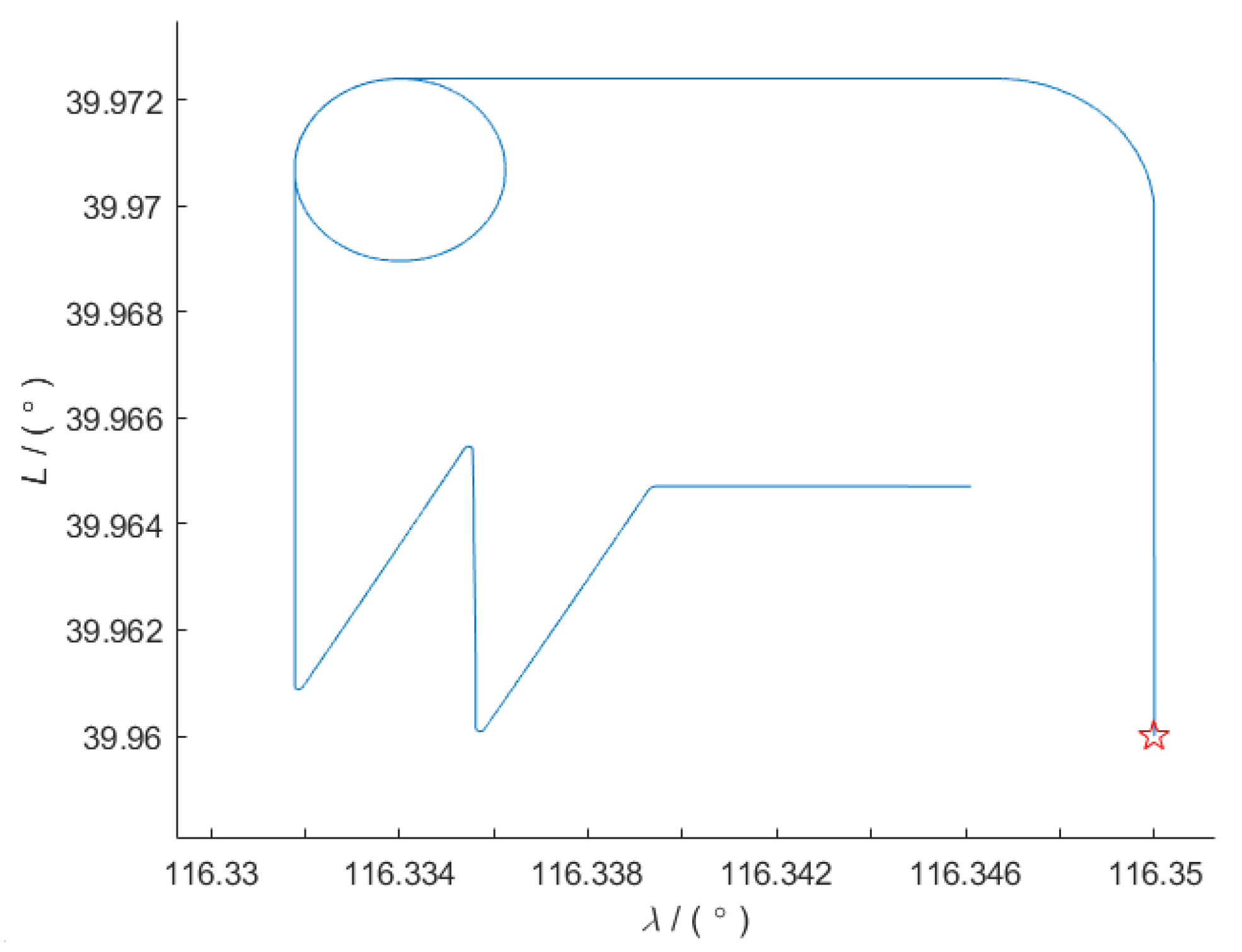
To validate the algorithm proposed in this paper, a trajectory is designed that includes various typical operating states, such as straight driving, acceleration, slow turns, sharp turns, and circular motion. The total duration of the trajectory is 1066 s, and the actual trajectory is shown in Figure 1’s trajectory chart, with the starting point marked by a red star. To ensure comprehensive validation, the designed trajectory covers various common navigation scenarios. At 300 s, GNSS data is corrupted with a 10 s error and 2 times the measurement variance, and at 500 s, GNSS data is corrupted with a 50 s error and 3 times the measurement variance. This is intended to test the algorithm’s robustness and accuracy in different dynamic environments.

The algorithm in this paper uses the “East–North–Up” (ENU) coordinate system. The initial position is 39.96° (N), 116.35° (E), and 45 m; the initial pitch, roll, heading angles, and velocity are all 0. The inertial navigation data frequency is 100 Hz, and the GNSS observation frequency is 1 Hz. The initial three-dimensional position errors are 2 m, 2 m, and 5 m, and the three-dimensional attitude angle errors are [1°, 1°, 10°]. The three-dimensional velocity error is 0.1 m/s, and the GNSS measurement variance is [1, 1, 3]. The parameters of the inertial measurement unit are shown in

Table 1. Main sensor parameters.

Sensor	Bias	Random Walk
Gyroscope	$0.3°/\mathrm{h}$	$0.01°/\sqrt{\mathrm{h}}$
Accelerometer	$100 \mathsf{\mu }\mathrm{g}$	$5 \mathsf{\mu }\mathrm{g}/\sqrt{\mathrm{H}\mathrm{z}}$

.

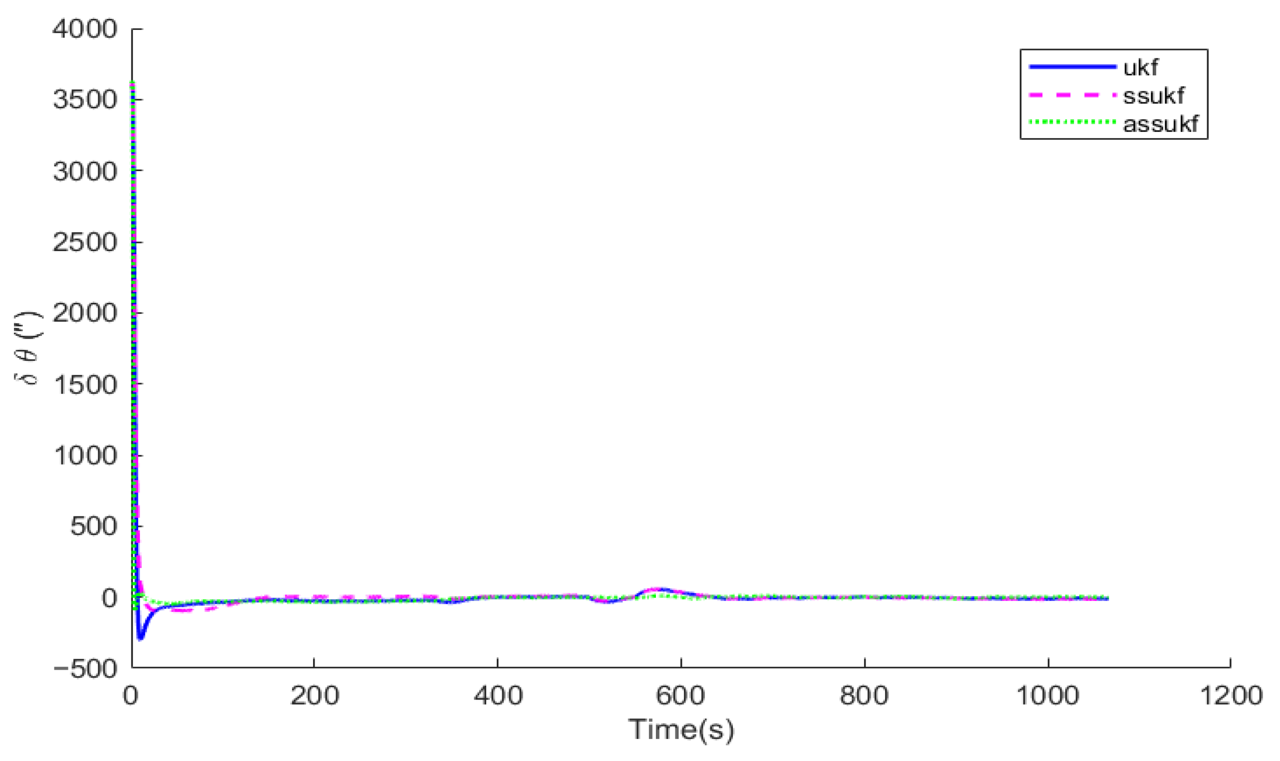
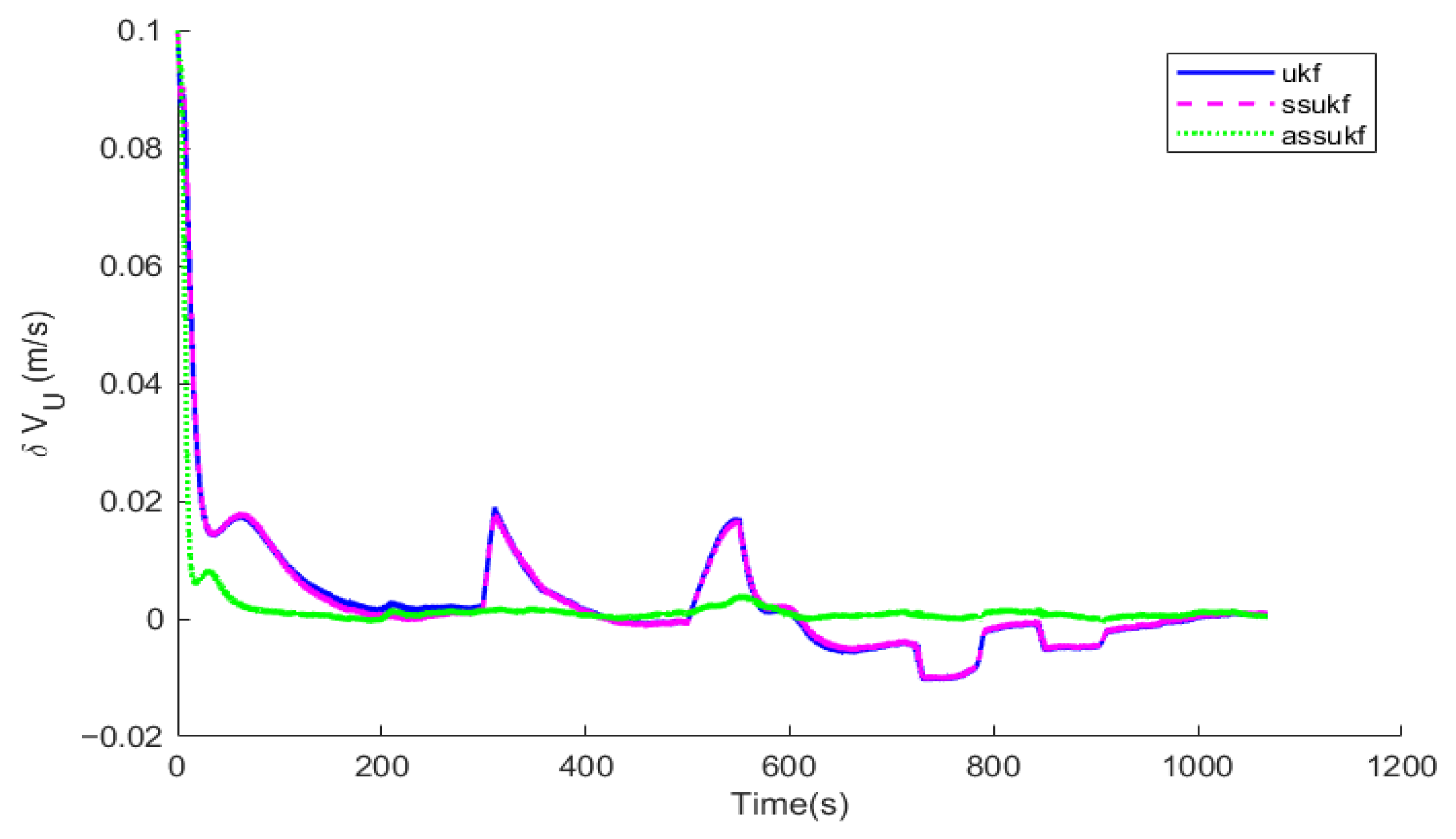
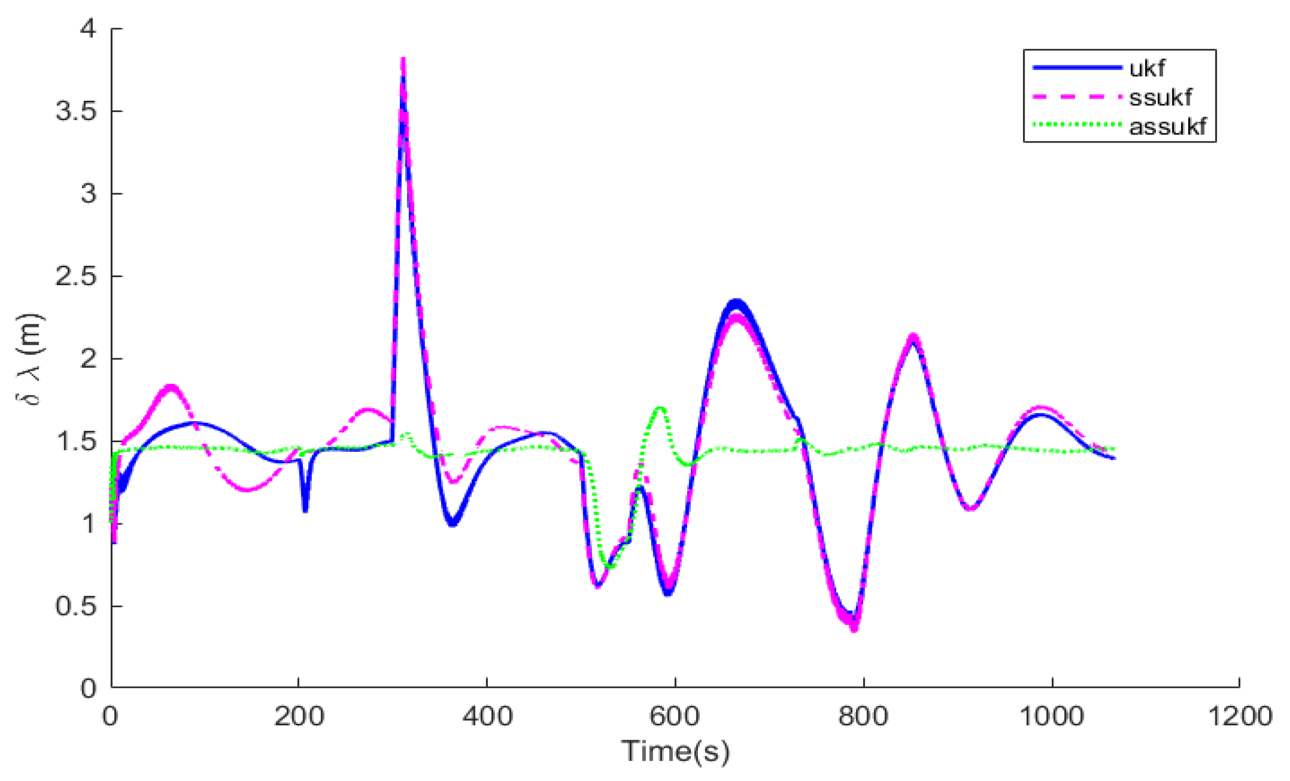
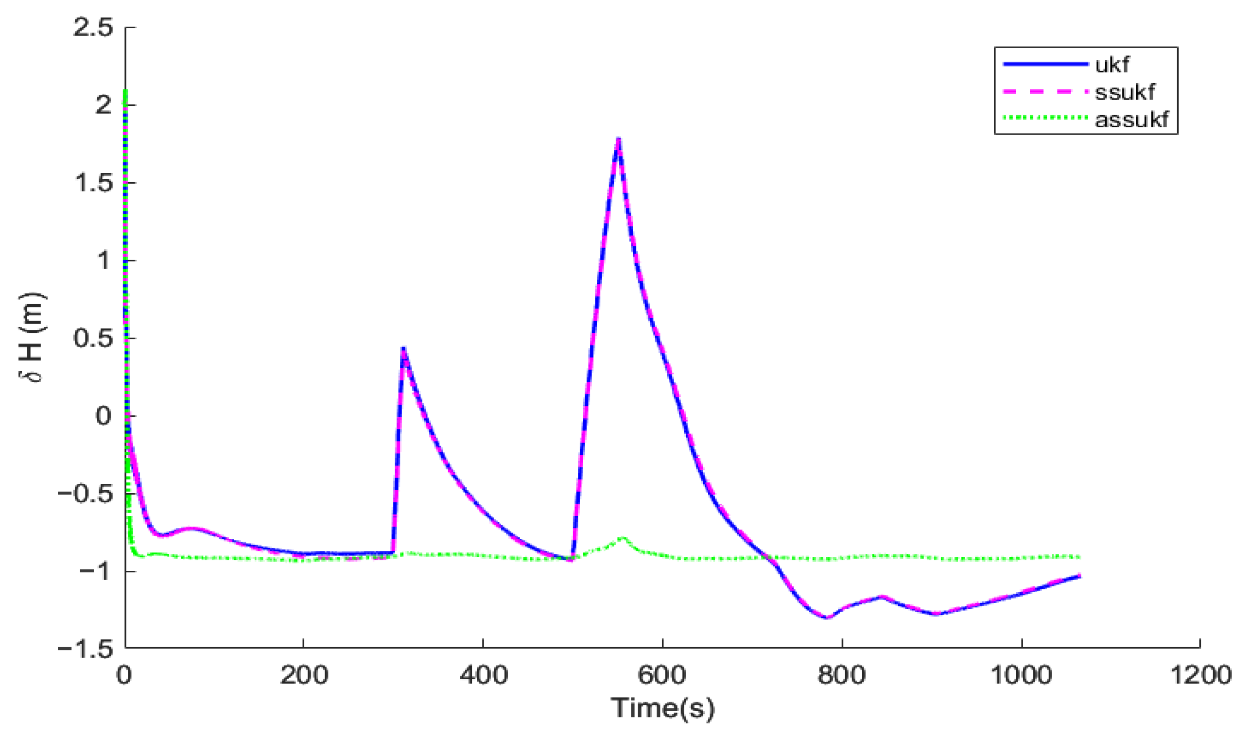
Under the same simulation conditions, the same set of IMU and GNSS simulation data are selected to perform simulations for the Unscented Kalman Filter (UKF), the Simplified Spherical Unscented Kalman Filter (SSUKF), and the Adaptive Simplified Spherical Unscented Kalman Filter (ASSUKF) proposed in this paper. The algorithms’ running times are compared, and corresponding comparison curves of attitude error, velocity error, and position error are plotted.

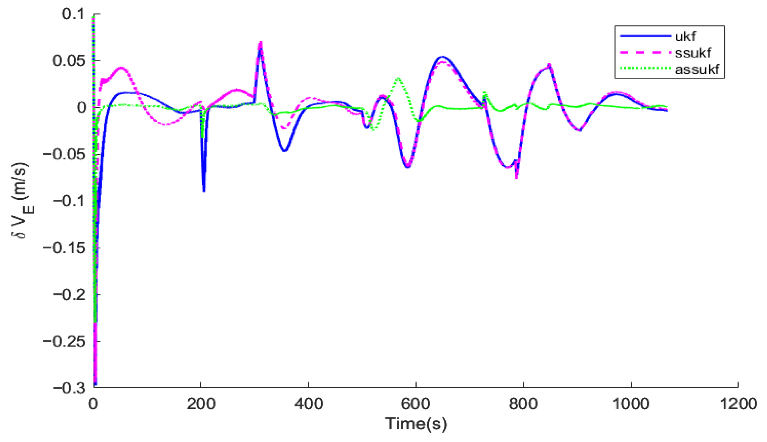
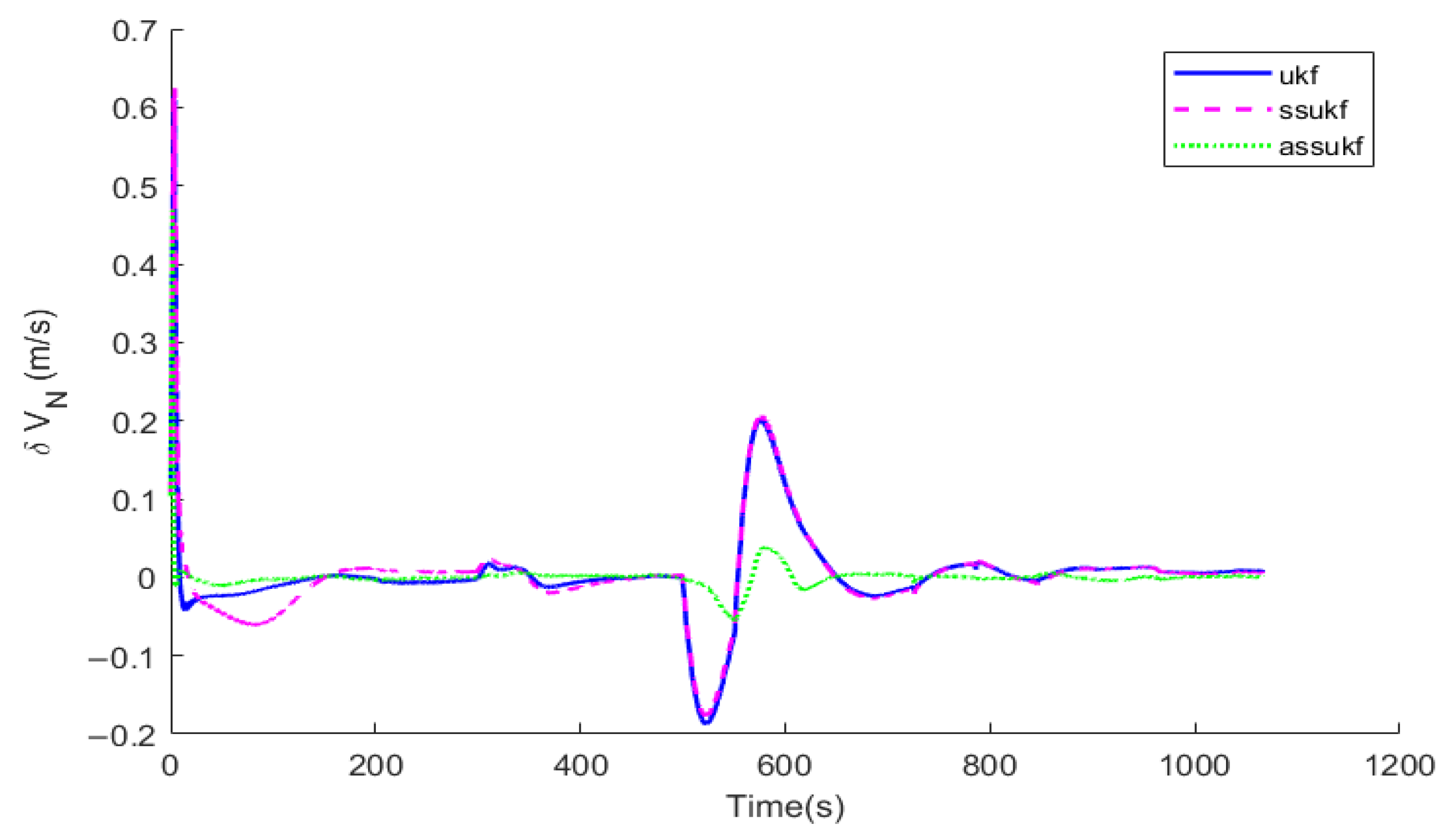
As can be seen from Figure 2, Figure 3, Figure 4, Figure 5, Figure 6, Figure 7, Figure 8, Figure 9 and Figure 10, in terms of attitude, velocity, and position, ASSUKF exhibits smaller errors and more stable fluctuations, with overall performance superior to the other two methods. Different measurement errors were set at 300 s and 500 s, causing fluctuations at these specific time points for all three methods. Among them, the attitude error shows relatively minor fluctuations, while the three-axis velocity error fluctuates at 300 s and 500 s but gradually converges, with ASSUKF showing significantly smaller fluctuations and faster convergence. The larger fluctuations in velocity errors during the remaining time are due to filtering errors caused by the measurement data. From these points, it can also be observed that ASSUKF effectively identifies and corrects these errors, ensuring the accuracy of the filtering process. Similar fluctuations are seen in the position error, but ASSUKF provides a smoother result with smaller errors, indicating that ASSUKF can maintain stable estimation results in complex dynamic environments and significantly reduce the error magnitude. Compared to the standard UKF, ASSUKF demonstrates stronger adaptability and robustness.

The standard UKF, due to its lack of noise estimation capability, cannot promptly and accurately perceive changes in GNSS measurement noise, leading to significant deviations in the filter’s estimation results when such changes occur. In contrast, ASSUKF, by introducing an adaptive noise estimation mechanism, can continuously monitor and precisely estimate changes in GNSS measurement noise. The adaptive factor enables ASSUKF to dynamically adjust the noise covariance matrix based on real-time observational data, thereby better adapting to different noise environments. Through this mechanism, ASSUKF not only effectively handles dynamic noise variations but also maintains high-precision state estimation under various complex environmental conditions, significantly reducing navigation errors.

To further validate the reliability of the results and avoid errors caused by random factors in a single trial, we conducted ten independent trials, each using the same parameter settings. For each trial, the measurement errors followed the same distribution. We then compiled the relevant experimental results and averaged the outcomes of the ten trials.

Table 2. Comparison of root mean square errors (RMSE) for different algorithms.

Filter	Position Error/m			$\mathbf{Velocity} \mathbf{Error}/\mathbf{m}\cdot {\mathbf{s}}^{-1}$			Attitude Error/(″ ″ ′)
	$∆\mathit{L}$	$∆\mathit{\lambda }$	$∆\mathit{H}$	$∆{\mathit{V}}_{\mathit{E}}$	$∆{\mathit{V}}_{\mathit{N}}$	$∆{\mathit{V}}_{\mathit{U}}$	$∆\mathit{\theta }$	$\mathbf{∆}\mathsf{\gamma }$	$∆\mathit{\psi }$
UKF	1.04	1.78	2.31	0.093	0.077	0.012	132.4	190.4	76.4
SSUKF	1.06	1.82	2.32	0.093	0.079	0.012	131.5	167.0	152.6
ASSUKF	0.86	1.43	2.24	0.092	0.074	0.007	95.9	133.5	115.5

, comparison of root mean square errors (RMSEs) for different algorithms, shows the Root Mean Square Error (RMSE) of the navigation results for the three methods. In terms of position error, UKF and SSUKF have similar accuracy, while ASSUKF, with the addition of adaptive filtering, effectively handles abnormal noise and significantly improves accuracy. Specifically, ASSUKF improves position accuracy in the latitude direction by 18.10% and in the longitude direction by 20.6%. Regarding velocity error, the velocity estimation capabilities of the three methods are relatively similar, with good accuracy. For attitude error, ASSUKF performs exceptionally well. Specifically, the pitch angle error improves by 27.6% compared to UKF and by 27.1% compared to SSUKF. The roll angle error improves by 29.9% compared to UKF and by 20.1% compared to SSUKF. The heading angle error improves by 24.3% compared to SSUKF but is slightly worse than UKF. By comparing the RMSEs of UKF, SSUKF, and ASSUKF, it is clear that the proposed ASSUKF significantly outperforms both UKF and SSUKF in terms of position and attitude accuracy. The introduction of the adaptive factor effectively improves the filtering accuracy of the integrated navigation system, ensuring that the system provides more accurate and reliable navigation results in complex dynamic environments.

Another important metric for evaluating the algorithm is its running efficiency. While the UKF is relatively simple in implementation, it requires direct handling of the covariance matrix and its inversion operations, which results in higher computational complexity, especially when dealing with high-dimensional systems or environments with significant noise variations. This makes UKF’s run time noticeably longer, particularly when the state dimension is large. In contrast, SSUKF and ASSUKF use the spherical simplex sampling strategy, which effectively reduces numerical instability and memory consumption. These methods improve running efficiency while maintaining high accuracy.

Table 3. Comparison of running times for different algorithms.

Filter	UKF	SSUKF	ASSUKF
Running Time (s)	48.90	23.53	23.20

, comparison of running times for different algorithms, shows the running times of the three algorithms.

5. Conclusions

In response to the issue of the standard UKF algorithm requiring precisely known prior statistical information about measurement noise, this paper conducts an in-depth analysis of the limitations of traditional algorithms and proposes a UKF algorithm based on an adaptive factor. This algorithm introduces an adaptive mechanism that can estimate changes in measurement noise in real time and dynamically adjust the noise covariance matrix. It ensures accurate and real-time estimation of measurement noise changes while maintaining efficiency, avoiding the issues of filter divergence or accuracy degradation caused by inaccurate noise estimation. The simulation results show that ASSUKF improves accuracy by 18.10% in the latitude direction and 20.6% in the longitude direction. In terms of attitude errors, ASSUKF improves the pitch angle error by 27.6% compared to UKF and by 27.1% compared to SSUKF. The roll angle error is improved by 29.9% compared to UKF and by 20.1% compared to SSUKF. The heading angle error is improved by 24.3% compared to SSUKF. These results demonstrate the excellent filtering performance of ASSUKF. Although ASSUKF performs excellently in simulations, it lacks validation with real-world data. Its performance in practical applications may be influenced by various factors. In the future, it would be beneficial to collect data from real-world environments to verify the stability and robustness of the proposed algorithm in complex settings.