A Planer Moving Microphone Array for Sound Source Localization

Abstract

Sound source localization (SSL) equips service robots with the ability to perceive sound similarly to humans, which is particularly valuable in complex, dark indoor environments where vision-based systems may not work. From a data collection perspective, increasing the number of microphones generally improves SSL performance. However, a large microphone array such as a 16-microphone array configuration may occupy significant space on a robot. To address this, we propose a novel framework that uses a structure of four planar moving microphones to emulate the performance of a 16-microphone array, thereby saving space. Because of its unique design, this structure can dynamically form various spatial patterns, enabling 3D SSL, including estimation of angle, distance, and height. For experimental comparison, we also constructed a circular 6-microphone array and a planar 4 × 4 microphone array, both capable of rotation to ensure fairness. Three SSL algorithms were applied across all configurations. Experiments were conducted in a standard classroom environment, and the results show that the proposed framework achieves approximately 80–90% accuracy in angular estimation and around 85% accuracy in distance and height estimation, comparable to the performance of the 4 × 4 planar microphone array.

1. Introduction

With the recent advent of sound source localization (SSL) technology, it has been used in many different terminals, such as those pertaining to radars, headsets, service robots, and so on. In daily life, SSL could supplementarily assist audio conception for vision-driven applications [1]. However, when people talk about hearing ability, they are usually referring to direction recognition ability. Distance estimation is much less emphasized, since the human auditory system cannot estimate distance as accurately as direction [2,3]. This is especially true for scenarios relating to indoor human and robot interaction at dawn, at dusk, and in the evening, when the lighting conditions are not sufficient for distance estimation, meaning direction estimation is severely degraded due to the sole reliance on visualization.

SSL provides robots with an ability to hear from humans and know where the orders are coming from [1]. In the field of conventional SSL, many researchers have explored the relationships between various acoustic cues, discussing aspects such as spectral variance [2], inter-time difference (ITD), inter-level difference (ILD) [4], time difference of arrival (TDOA) [5], and the direct power-to-reverberant power ratio (DRR) [6]. For huge microphone arrays, beamforming-based methods have been developed. In beamforming-based methods, a beamformer is constructed by the steered response power with phase transform (SRP-PHAT) to sum the generalized cross-correlation phase transform (GCC-PHAT) [7]. SRP-PHAT improves the ability to remain robust against reverberant noise by utilizing the fault tolerance of multiple microphones. Considering the huge calculation load, SRP-PHAT has been optimized by numerous researchers [7,8]. Subspace-based methods like multiple signal classification (MUSIC) represent other famous SSL methods. The MUSIC method decomposes the received signal covariance matrix into one called signal subspace and one called noise subspace and uses the orthogonality of the two spaces to find the peak of planar direction of the sound source [9,10,11,12,13,14]. Similarly to SRP-PHAT, MUSIC requires a large amount of computation sources. At the same time, it requires a large-volume microphone array to ensure the SSL accuracy [15].

In addition to single-sound source localization, spatial spectrum processing [16,17,18] and time–frequency (TF) processing is effective when dealing with multi-target sound source localization. TF processing methods can localize the direction of multiple sound sources and count the total number of sound sources. These TF processing methods assume that, at most, one source is dominant over the others in the TF domain, factoring in the sparse property of speech signals. This assumption, also called the W-disjoint orthogonal (WDO) assumption [18], can simplify multiple-source localization on broadband to single-source localization in individual TF bins.

However, when these algorithms are applied to a multiple-microphone array, around 16 microphones and a huge volume are required to ensure excellent performance. Special headsets have been designed for noise cancellation, as evidenced by [19,20,21], wherein researchers built a healthcare headset for children with autism spectrum disorder. These kinds of structures are hard to integrate practically in service robots. The researchers then derived solutions based on two perspectives: the first focused on building a smaller microphone array, while the second focused on building an active microphone array.

The key idea behind making an active microphone array is to collect more data for processing. Before designing an active microphone array, first, researching human head rotation’s impact on sound source collection is essential. In [22], H. Chen et al. investigate the performance robustness of an active headrest with virtual microphones against head rotation in a pure-tone-diffracted diffuse sound field. Similarly, to gain insight into the passive rotation of sound sources, in [23,24,25], the researchers focused on how acoustic factors can be estimated from sound sources rotating around signal receivers. Then, considering the rise in prominence of unmanned aerial systems (UASs), they drew conclusions based on noise generated from propellers rotating. In [26], M. Heydari et al. found that the UAS noise increases with pitch angles and the propellers’ rotating velocity, but an irregular trend with vehicle speed was also shown.

In addition to conducting research on the passive rotation of sound sources, researchers have also built active microphone arrays for acoustic research. In [27], Y. Wakabayashi et al. built a circular microphone array and rotated it to a certain degree to ensure optimized sound collection. In addition, they developed an interpolation algorithm so that they could collect virtual data, focusing on sound collected before and after rotation. In [24], Gala D. et al. directly used a linear rotating microphone array mounted on an unmanned vehicle. In [25], Zhong. et al. mounted a binaural microphone on a service robot for SSL. The linear microphone array featured in this study is always rotating and collecting data for a machine learning network to predict where the speaker is. With moving [28,29] and rotating microphone arrays [30,31] collecting more data, the proposed system could not only form a linear array pattern but also form other special patterns to carry out 2D to 3D localization. In [32,33,34], indoor 3D sound source localization is accomplished by fixing microphones to walls and the corners of rooms while a four-planar moving microphone structure occupies a much smaller space. Providing height information could also enrich data or evidence for speech recognition. For example, a child and an adult would speak at different levels in a relatively dark room at nightfall. Height information would have better performance than pure vision judgement [35,36].

Although the active microphone arrays mentioned above fulfilled their expectations, these arrays generally require a huge volume and lack the ability for height localization. That is to say, their SSL ability is 2D-based, not 3D-based. For this reason, this work proposes a four-planar moving microphone structure (FPMMS) to mimic a 16-microphone array, which has much smaller volume.

A validation experiment was conducted in a normal classroom. For a fair comparison, we also built a 4 × 4 microphone array, a circular 8-microphone array, and a 1 × 4 microphone linear array as contrast groups. Since FPMMS can move in planar, the arrays in the contrast groups can all rotate around their centers to collect more data. This work describes results in terms of angular estimation accuracy, horizontal distance estimation accuracy, and vertical height estimation accuracy.

The remainder of this paper is structured as follows: Section 2 introduces the FPMMS and describes the procedure carried out to build it. In Section 3, the FPMMS is compared with a linear rotating microphone array, a circular rotating microphone array, and a 16-microphone array. Finally, Section 4 presents the conclusions drawn from our research.

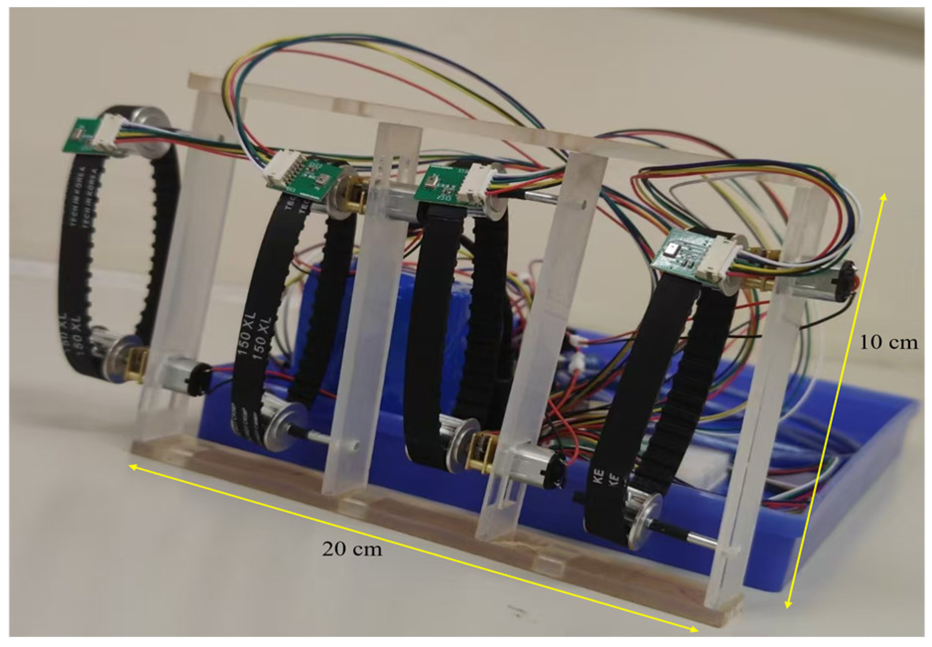
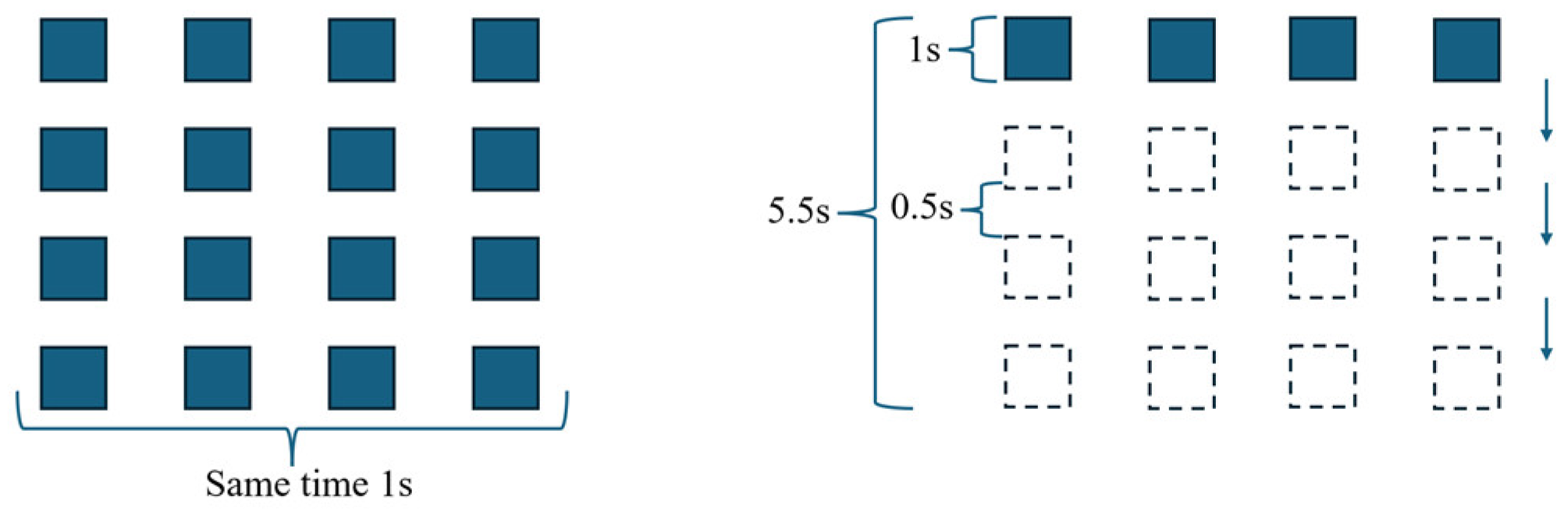
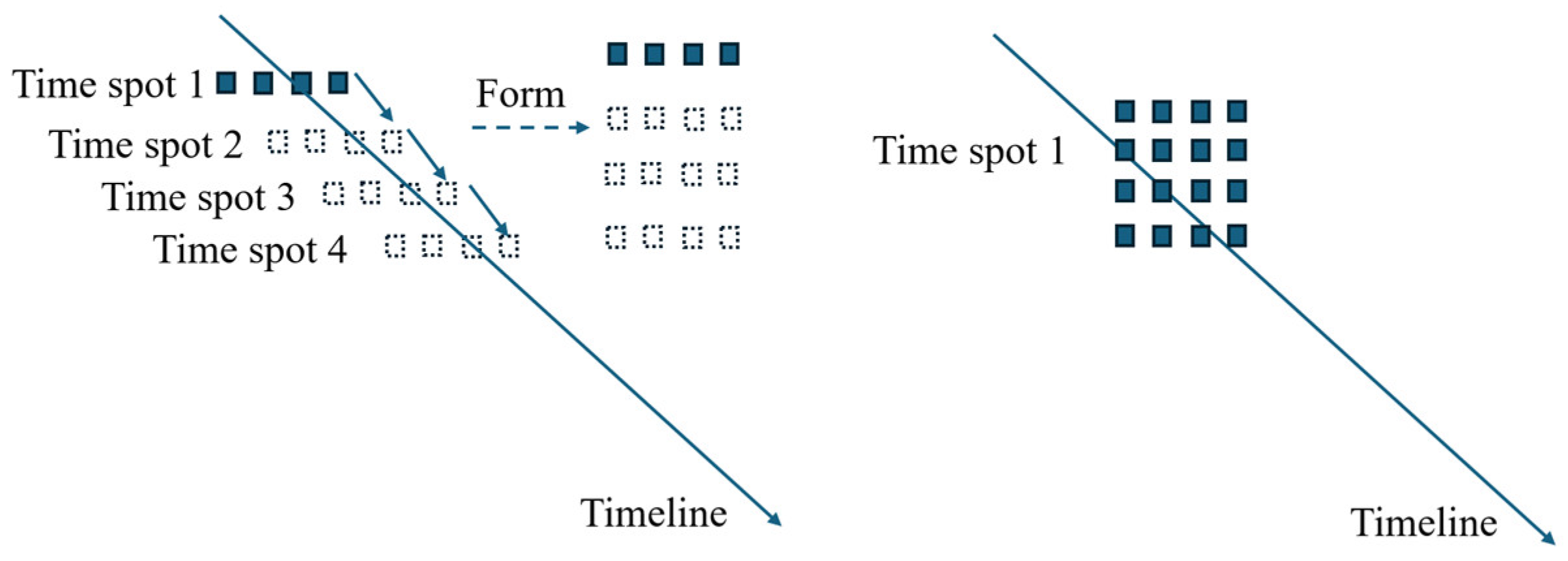
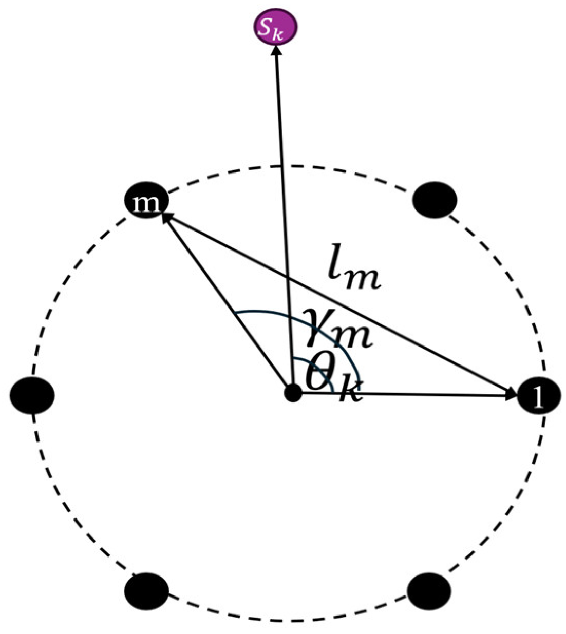
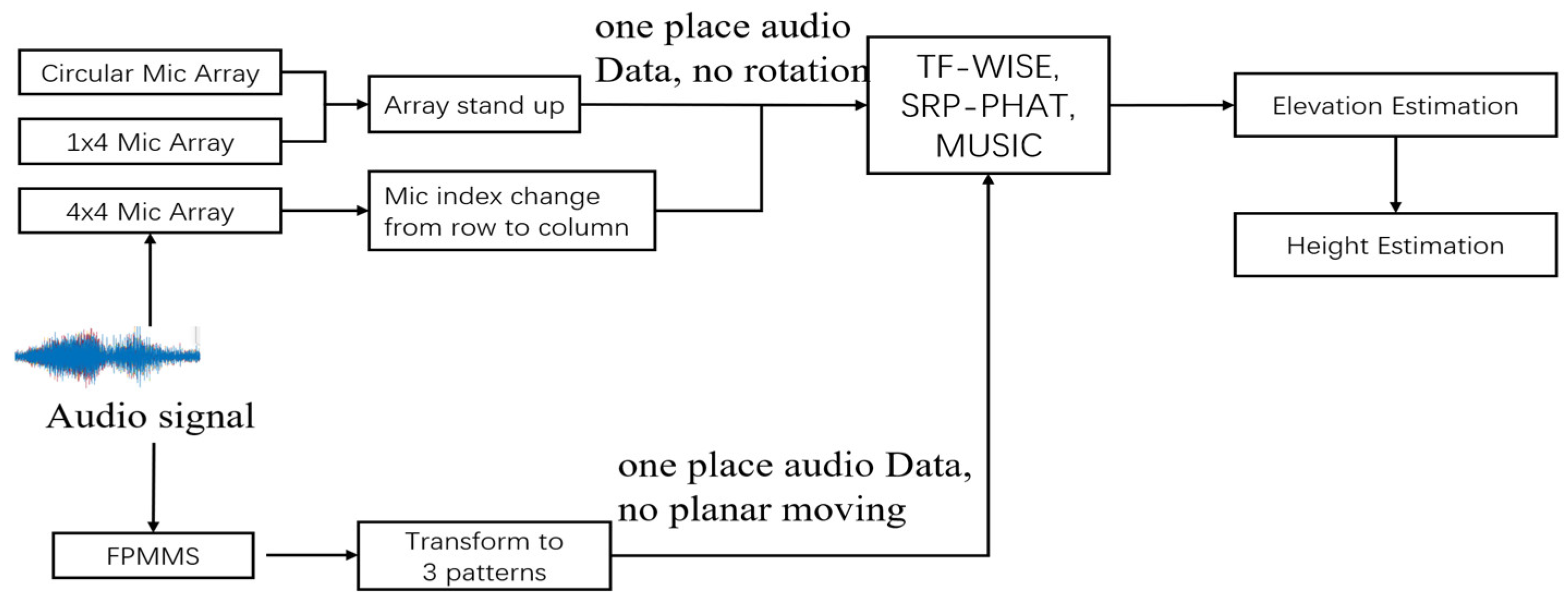
2. Introduction to the FPMMS and Building Procedure

As stated in the Introduction, we set out to develop an active microphone array. The key idea behind this structure is to collect more data for analysis and save space, since usual microphone arrays occupy a lot of space [37,38]. Considering that the structure was to be mounted on to the head of a service robot, we designed the following structure.

As Figure 1 displays, four MEMS microphones are placed separately on four conveyor belts, and four conveyor belts are driven separately by four small motors. The inter-mic distance is 6.67 cm. An Arduino circuit controls motor movement and direction. Thus, we could write scripts to move each microphone to any place precisely in the range of frame. The procedure required for the FPMMS to mimic a 16-microphone array is displayed in the flow chart below.

Figure 2 describes the audio data collected at each time spot, which are merged by the time index and not overlaid together. Figure 3 more specifically displays the procedure timeline. As shown on the right of Figure 3, a 4 × 4 microphone array collects data in 1 s (16-channel data). As shown on the left of Figure 3, the FPMMS comprises a 4-time, 1 s, 4-channel data collection structure.

Starting with angle estimation, we will gradually show the theory behind the FPMMS 3D SSL procedure. The signal received by the $m_{th}$ microphone in FPMMS can be modelled as follows:

$$x_m\left(t\right)={\sum }_{k=1}^K{\alpha }_{m,k}{s}_k\left(t-{\tau }_{m, {\theta }_k}\right)+{\upsilon }_m\left(t\right)$$

(1)

Here, $m\in \{\mathrm{1,2},\dots ,M\}$ is the microphone index number. For FPMMS, $M=4$. For the circular microphone array, $M=6$. For the 4 × 4 microphone array, $M=16.$ $k$ is the sound source index, and $K=2,3,4,5$. $s_k\left(t\right)$ is the sound uttered from the $k_{th}$ sound source. ${\tau }_{m, {\theta }_k}$ denotes the delay from the $k_{th}$ sound source to the $m_{th}$ microphone induced by ${\theta }_k$. ${\theta }_k$ is the horizontal angle observed from the top side in an anticlockwise manner. ${\upsilon }_m\left(t\right)$ is the assumed uncorrelated additive ambient noise received by the $m_{th}$ microphone. ${\alpha }_{m,k}$ represents the propagation attenuation factor from the $k_{th}$ sound source to the $m_{th}$ microphone.

Applying short-time Fourier transformation (STFT) to Equation (1), the signal in the $m_{th}$ microphone can be modelled in the time–frequency (TF) domain:

$$X_m\left(n,f\right)={\sum }_{k=1}^K{\alpha }_{m,k}{S}_k\left(n,f\right)e^{-j{\omega }_f{\tau }_{m, {\theta }_k}}+V_m(n,f)$$

(2)

where $n$ is the time frame index number, $f$ is the frequency band index number, and ${\omega }_f$ is the angular frequency of the $f_{th}$ frequency band. $X_m\left(n,f\right)$, $S_k\left(n,f\right)$, $V_m(n,f)$ denote the STFT coefficients of $x_m\left(t\right)$, $s_k\left(t\right)$, ${\upsilon }_m\left(t\right)$.

Since the array discussed herein requires synthesis of the signals received from the microphone for latter processing, Equation (2) can be rewritten into a vector form:

$$x\left(n,f\right)={\sum }_{k=1}^K{S}_k\left(n,f\right)\mathit{e}(f, {\theta }_k)+\mathit{v}(n,f)$$

(3)

Here,

$$x\left(n,f\right)={\left[X_1\left(n,f\right),X_2\left(n,f\right),\dots ,X_M\left(n,f\right)\right]}^T,$$

$$v\left(n,f\right)={\left[V_1\left(n,f\right),V_2\left(n,f\right),\dots ,V_M\left(n,f\right)\right]}^T,$$

$$e\left(f,{\theta }_k\right)={\left[{\alpha }_{1,k}{e}^{-j{\omega }_f{\tau }_{1, {\theta }_k}},\dots ,{\alpha }_{M,k}{e}^{-j{\omega }_f{\tau }_{M, {\theta }_k}}\right]}^T$$

The ${\alpha }_{m,k}$ is assumed to be identical and represented by $\alpha$. For all the microphone arrays, we chose the first microphone as the reference. The steering vector can be written as

$$e\left(f,{\theta }_k\right)=\alpha e^{-j{\omega }_f{\tau }_{1, {\theta }_k}}\times {[1,e^{-j{\omega }_f{(\tau }_{2, {\theta }_k}-{\tau }_{1, {\theta }_k})},\dots ,e^{-j{\omega }_f{(\tau }_{M, {\theta }_k}-{\tau }_{1, {\theta }_k})}]}^T$$

(4)

For all linear microphone arrays, including the FPMMS, 1 × 4 microphone array, 4 × 4 microphone array, and the circular microphone array, the relative time delay can be calculated as follows:

$${\tau }_{m, {\theta }_k}-{\tau }_{1, {\theta }_k}={\displaystyle \frac{d_{m,{\theta }_k}-d_{1,{\theta }_k}}{c}}$$

(5)

$d_{m,{\theta }_k}$ is the distance from the $k_{th}$ source to the $m_{th}$ microphone, and $d_{1,{\theta }_k}$ is the same for the $1_{st}$ reference microphone. $c$ is the sound speed. The only special adjustment for the circular microphone array is as follows:

$${\displaystyle \frac{d_{m,{\theta }_k}-d_{1,{\theta }_k}}{c}}={\displaystyle \frac{l_m\sin ({\gamma }_m/2-{\theta }_k)}{c}}$$

(6)

$l_m$, as shown in Figure 4, is the distance in the circular microphone array between the $m_{th}$ microphone and the $1_{st}$ reference microphone. ${\gamma }_m$ denotes the angle of the $m_{th}$ microphone to the $1_{st}$ reference microphone with respect to the center of the circle. For practical applications, ${\gamma }_m$ and $l_m$ can be calculated by the following geometrical relationships:

$${\gamma }_m=(m-1){\displaystyle \frac{2\pi }{M}}$$

(7)

$$l_m=2rcos\left({\displaystyle \frac{{\gamma }_m-\pi }{2}}\right)$$

(8)

Here, $r$ is the radius of the circular microphone array.

As shown in the flow chart, the four-time-collected data form together as a whole vector $\mathit{x}\left(n,f\right)$ and is sent to a TF-WISE algorithm [36] for multiple-sound source angular estimation.

For planar distance estimation, since the distance from the sound source to microphone $L$ is much smaller than ${\displaystyle \frac{2d^2}{\lambda }}$, $d$ is the inter-mic distance, and $\lambda$ is the wavelength. Thus, the near-field model is chosen [39,40]. Figure 5 depicts the procedure for the planar distance estimation model:

Here, $s$ is the sound source. The TF-WISE algorithm [41] gives time lag information, supposing that ${\tau }_{1, {\theta }_2},{\tau }_{1, {\theta }_3}$ represent the time lag between the first microphone (reference microphone), second microphone, and third microphone. The following relationships are formed:

$${\tau }_{1, {\theta }_2}={\displaystyle \frac{r_2-r_1}{c}}$$

(9)

$${\tau }_{1, {\theta }_3}={\displaystyle \frac{r_3-r_1}{c}}$$

(10)

where $r_1, r_2, r_3$ are the distances from the sound source to the microphones, and $c$ represents sound speed. Utilizing the law of cosines,

$$r_2^2=r_1^2+d^2+2r_{1}dcos{\theta }_1$$

(11)

$$r_3^2=r_1^2+{4d}^2+4r_{1}dcos{\theta }_1$$

(12)

${\tau }_{1, {\theta }_2}$, ${\tau }_{1, {\theta }_3}$, $d$, and $c$ are estimated or known values. Using Equations (1)–(4), $r_1, r_2, r_3$ and ${\theta }_1$ can be calculated. It should be clear that for angular estimation based on TF-WISE, the angle/geometry is for the center of the microphone array, while the ${\theta }_1$ here is the angle estimation for the reference microphone.

As for height estimation, we still utilize a near-field model. Apart from the first pattern, which will be discussed later, the remaining two patterns only have two microphones for time lag estimation, while distance estimation needs at least three microphones. The situation is simplified to the far field here, meaning that only the angle in the vertical surface can be estimated. Thus, we utilize the angle and distance estimated previously, fixing the sound source on the vertical axis. The FPMMS should only give a vertical surface angle $\phi$ estimation, and then, height estimation can be calculated with the following scheme.

Here, $H$ is the vertical height estimation. In Figure 6, $h$ is the known height of the microphone array mounted on the robot. $r$ is the result of previous planar distance estimation. $\phi$ denotes the angle estimated using the TF-WISE algorithm by different patterns of FPMMS, introduced below.

$$H=h+r\times \arctan \left(\phi \right)$$

(13)

We know that the perfect situation would involve one linear microphone array being vertical to the ground to estimate angles for height calculation [42] and parallel to the ground to estimate angles for distance estimation. The focus of this work is to find a balance between microphone array size and the array’s data collection quality. If we add a structure for FPMMS patterns completely vertical to the ground that occupy much more space can be formed. Thus, we proposed three patterns and tested them with respect to height estimation.

Apart from forming a linear microphone array to mimic a 16-microphone array, FPMMS can also form the following patterns.

In Figure 7, Figure 8 and Figure 9, these patterns are designed to carry out height estimation. For instance, in Figure 8a, we may utilize collected sound data to facilitate angle estimation, and then, the FPMMS would take the form shown in Figure 8b. Again, we could obtain another angle estimation; then, an average estimated angle would be used. With the estimated average angle combining the former direction and distance estimations, the height of the sound source can be calculated using Equation (13).

For different patterns, the inputs $\mathit{x}\left(n,f\right)$ are formed differently:

$${\mathit{x}}_{pattern1-pair1}\left(n,f\right)=[X_1\left(n,f\right),X_4\left(n,f\right)]$$

(14)

$${\mathit{x}}_{pattern1-pair2}\left(n,f\right)=[X_2\left(n,f\right),X_3\left(n,f\right)]$$

(15)

$${\mathit{x}}_{pattern2-pair1}\left(n,f\right)=[X_1\left(n,f\right),X_2\left(n,f\right)]$$

(16)

$${\mathit{x}}_{pattern2-pair2}\left(n,f\right)=[X_3\left(n,f\right),X_4\left(n,f\right)]$$

(17)

$${\mathit{x}}_{pattern3-pair1}\left(n,f\right)=[X_1\left(n,f\right),X_2\left(n,f\right)]$$

(18)

$${\mathit{x}}_{pattern3-pair2}\left(n,f\right)=[X_3\left(n,f\right),X_4\left(n,f\right)]$$

(19)

In the experiment, we tested the performance of the different patterns shown in Figure 7, Figure 8 and Figure 9. In the next section, we describe three further experiments. Each experiment corresponds to one of the following factors: direction estimation, planar distance estimation, and height estimation.

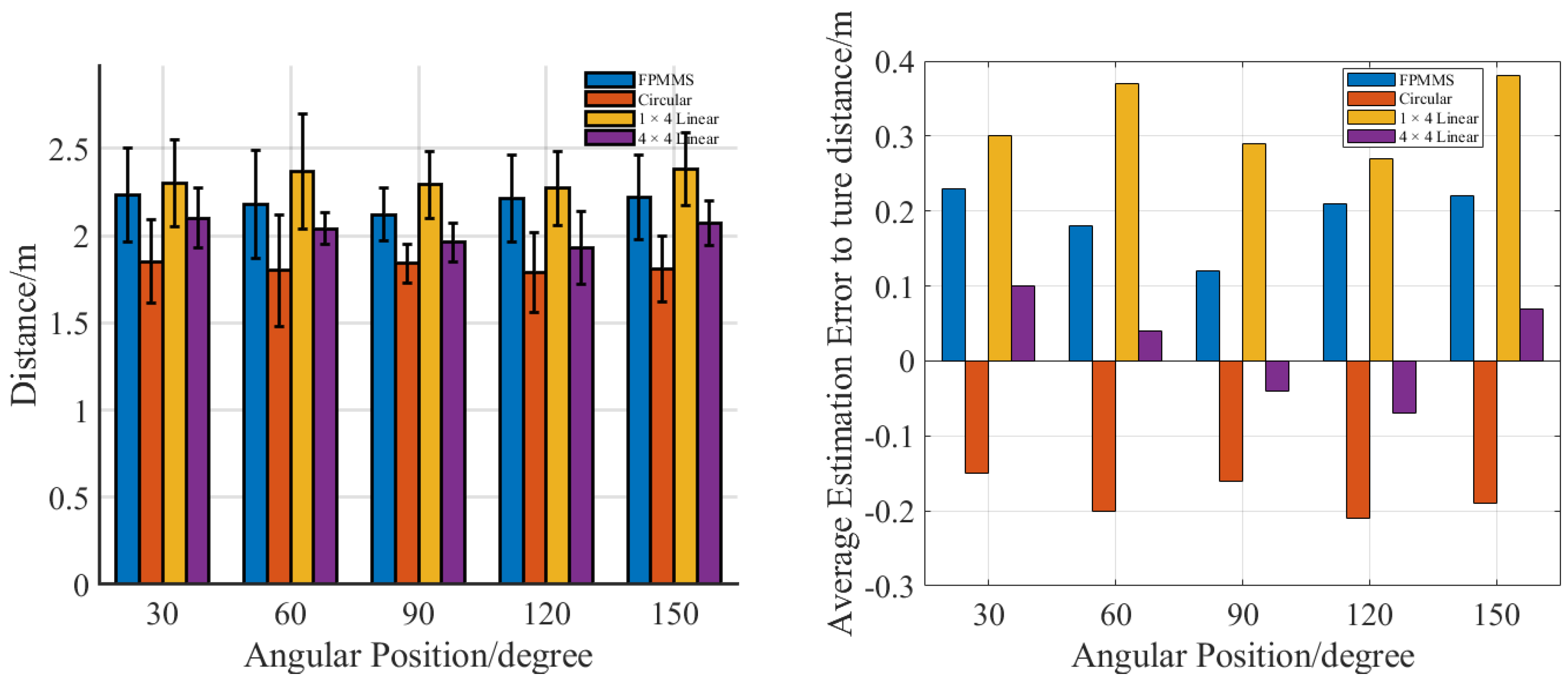
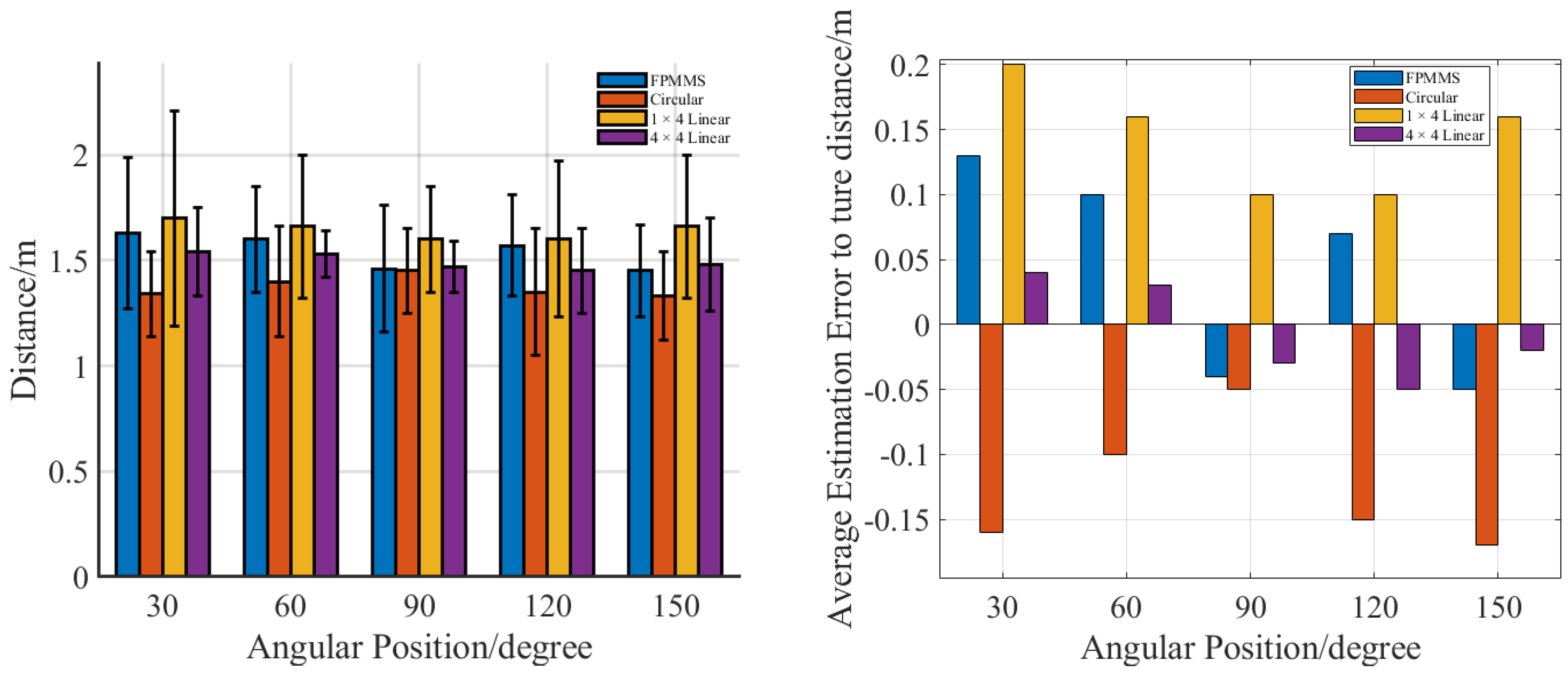
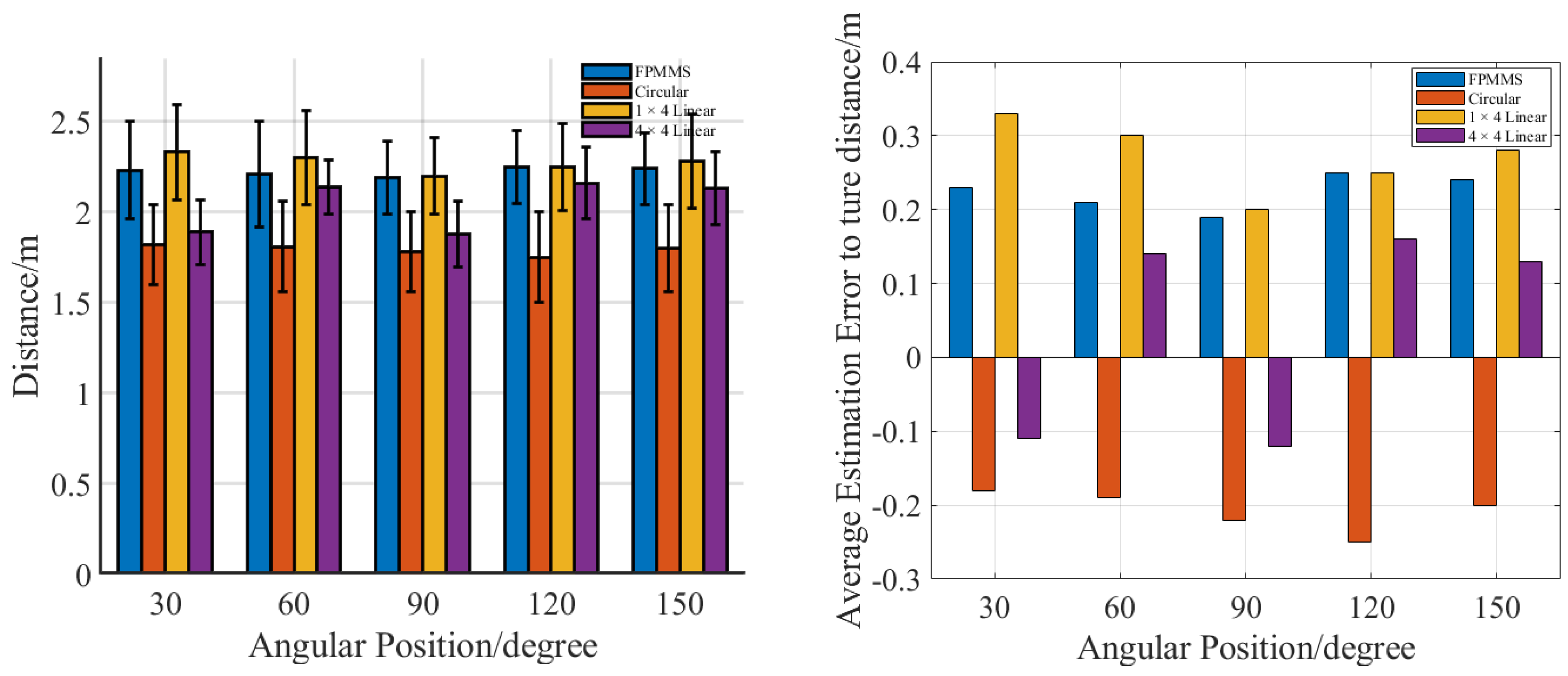
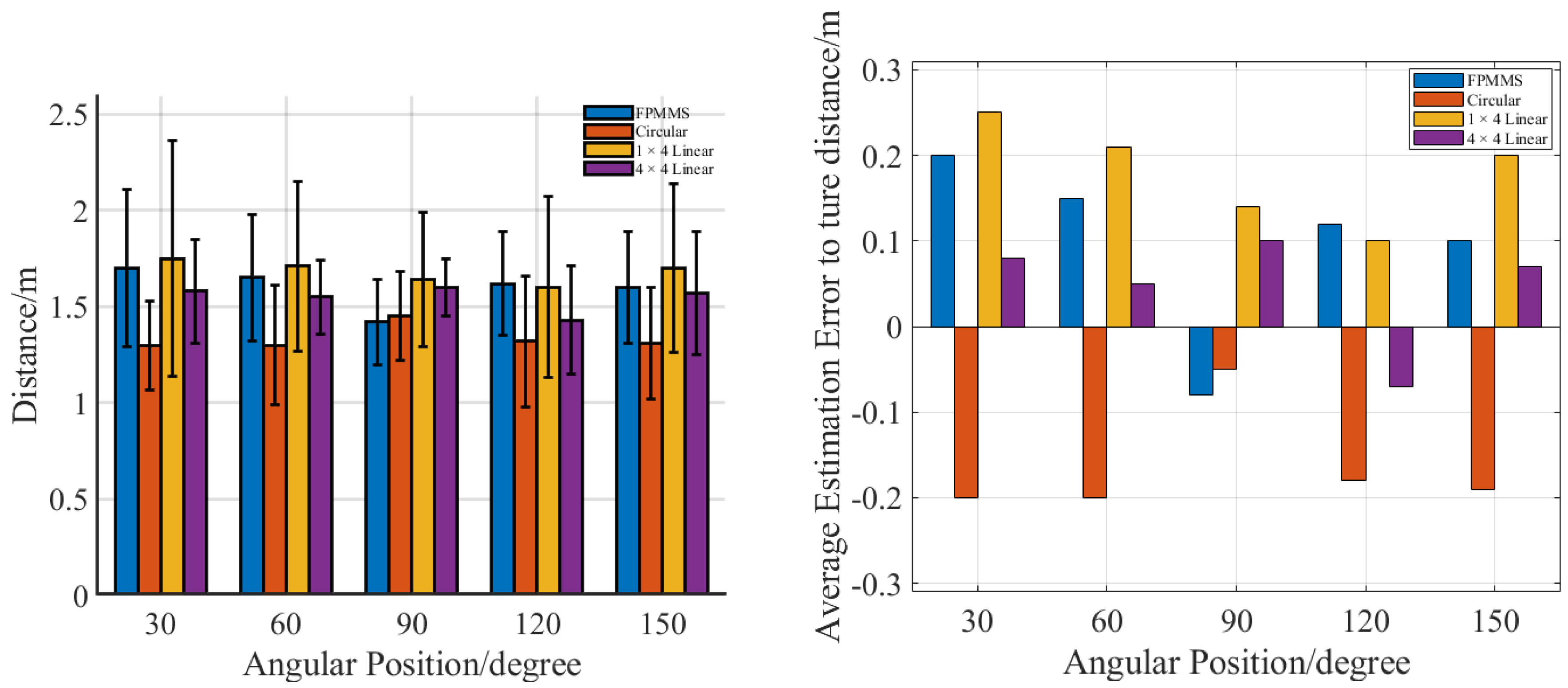
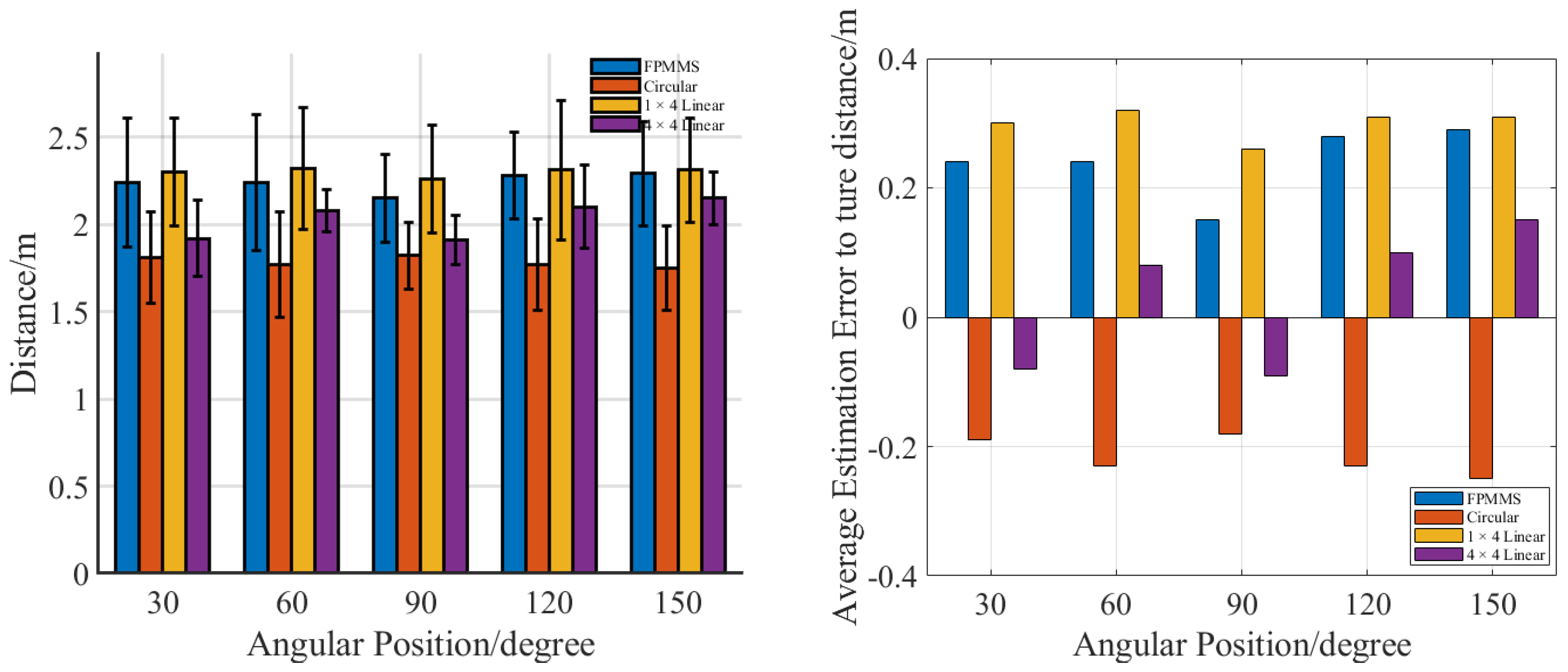
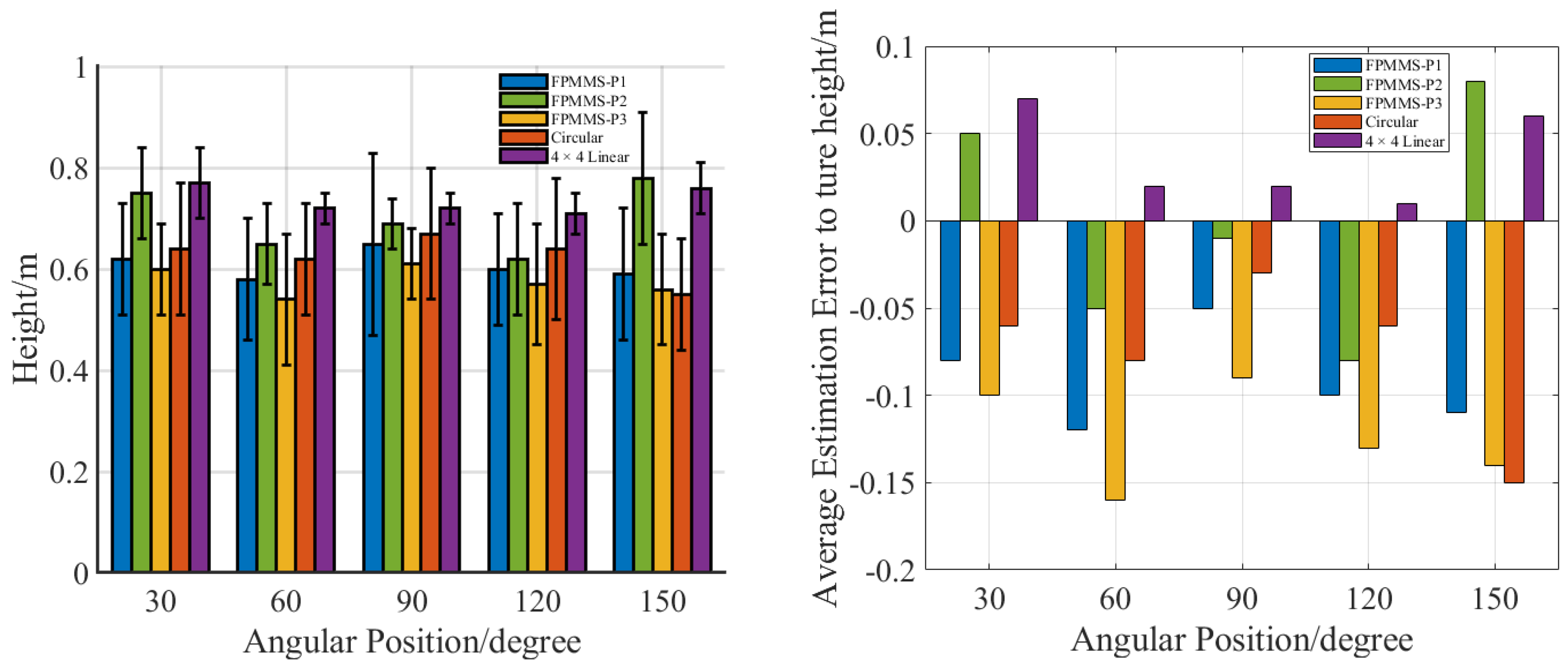
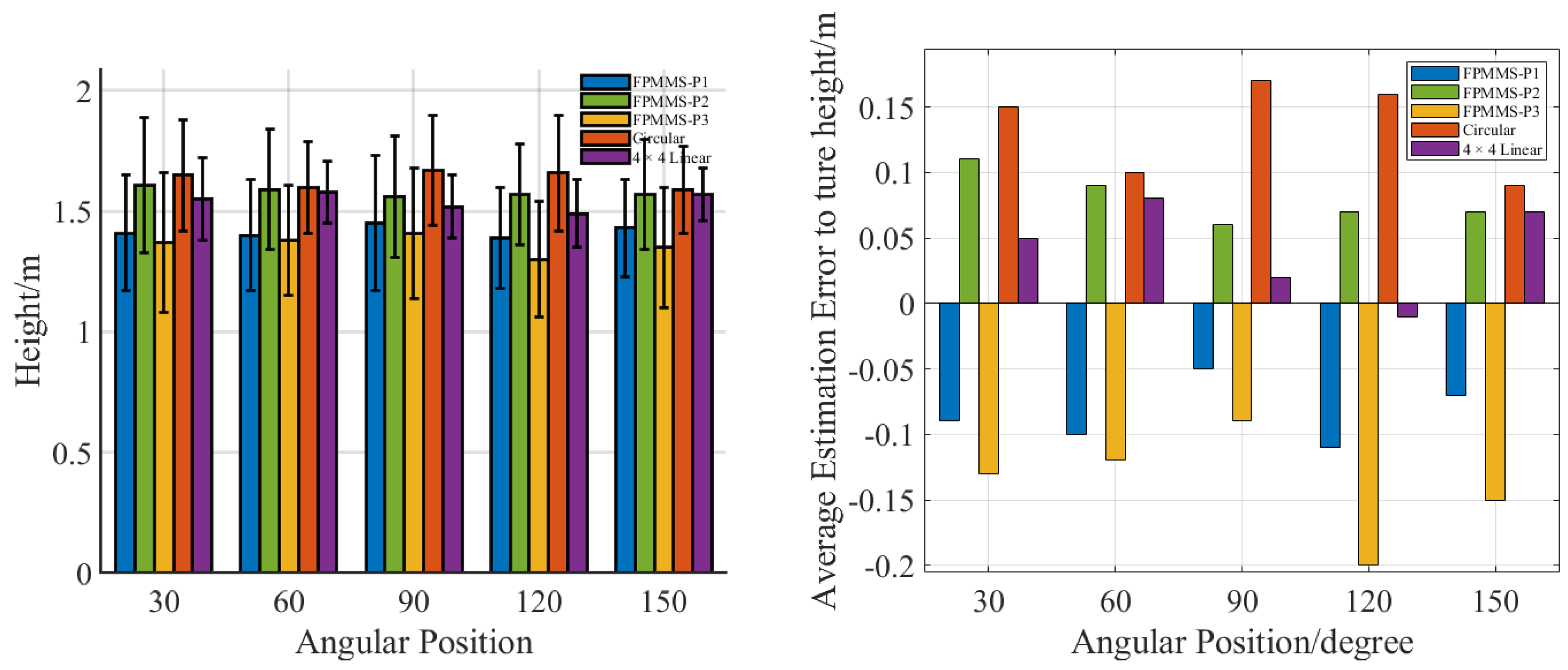
3. Experiment and Results

In this section, we describe an experiment conducted to compare the performance of FPMMS with a 1 × 4 linear rotation microphone array, a circular rotation microphone array, and a 4 × 4 rotation microphone array (summarized as the contrast groups). We also build the microphone array displayed in Figure 10 (left). In addition to the different active microphone arrays used for comparison, we also used three major SSL algorithms—TF-WISE, SRP-PHAT, and MUSIC—to assess the performance of the active microphone arrays. The signal used for the experiment was derived from the LibriSpeech dataset [43,44,45,46,47].

Three experiments, one each for azimuth, distance, and height, were conducted in one normal classroom, as depicted in Figure 10. The classroom was 8 m long, 10 m wide, and 3 m high. Each experiment was conducted in a very common classroom environment, with $T_{60}=240 \mathrm{m}\mathrm{s}$ and $SNR=15 \mathrm{d}\mathrm{B}$. In addition, for each experiment, we developed a corresponding flow chart to explain the procedures for direction, distance, and height estimation.

In Figure 11, the 1 × 4 microphone array uses one row of the 4 × 4 microphone array. The radius of the circular microphone array is 10 cm. The length of the 4 × 4 microphone array is 20 cm, and the height of the 4 × 4 microphone array is 15 cm, where the horizontal inter-mic distance is about 6.67 cm, and the vertical inter-mic distance is 5 cm.

All motors are synchronously controlled by high- and low-level clock signals emitted by the Arduino board, i.e., PWM-based control was used. Before the experiment, the speed of the conveyor belt with the matching gear under the maximum PWM power was measured (with the microphone installed). Based on this, the durations for which the high and low levels were required for translation and rotation were set. Continuous movement and sound acquisition would increase internal noise pollution. Due to the fixed timing control, the time interval positions of the microphone movement in the audio could be calculated from the sampling and timing, allowing them to be cut out. The Arduino board generates high-/low-level clock signals for PWM-based control. The Arduino’s internal clock and the configured baud rate (command transmission frequency) were also considered. This experiment used 9600 baud serial communication.

For the number of angle directions at the same distance, we chose K targets from five directions to form a multiple-sound source scenario. K is 2 and 3 here. For the angle directions at different distances, we picked K targets, but no direction was focused on; rather, we picked both 1.5 m and 2 m as the target at the same time. K was 2, 3, 4, or 5 for different distance cases. For the FPMMS, the movement time was 0.5 s, and the stationary time was 1 s, always facing directly forward relative to the robot. For the 1 × 4 and 4 × 4 microphone arrays, 0° was set as facing directly forward (robot front). The rotation angles, from left to right, were −15°, 0°, and 15°, with a rotation control time of 0.1 s and a stationary time of 1 s. For the circular microphone array, 0° was set with the first reference mic aligned to the robot’s front. The rotation angles, from left to right, were −15°, 0°, and 15°, with a rotation control time of 0.1 s and a stationary time of 1 s.

The first experiment focused on estimating the angle of multiple targets in multiple directions. The FPMMS result was compared with the ones derived from the contrast groups. FPMMS was mounted on a robot at a height of 1 m from the floor. The directions of the targets were 30°, 60°, 90°, 120°, and 150°. Sound sources were set at two different distances, 1.5 m and 2 m. Thus, unlike in [21], wherein the authors set only one distance, our multi-target system was more complex. Figure 12 depicts the procedure of the experiment.

The direction estimation results are shown below. The figures denote the gaps between each microphone array estimation result and the ground truth directions.

In Figure 13, Figure 14, Figure 15, Figure 16, Figure 17, Figure 18, Figure 19, Figure 20, Figure 21, Figure 22, Figure 23 and Figure 24, the horizontal axes represent location distances, and the polar axes are in degrees. From the results, we can see that, in angular estimation, FPMMS generally makes estimations that are much closer to the actual performance of a 16-microphone array than other forms of active microphone array. At 90°, FPMMS performs better than at other angles. The accuracy at a distance of 1.5 m is generally better than that at a distance of 2 m. FPMMS works better in all five directions and two distances than the 1 × 4 linear rotating microphone array. Regarding the different SSL algorithms, the TF-WISE group generally performs better, though it is not as useful in scenarios that feature fewer targets. When the number of targets is around three, four, or five, TF-WISE displays its advantages. In addition, the number of microphones affects each SSL algorithm’s recognition ability. In theory, TF-WISE, MUSIC, and SRP-PHAT can recognize “k − 1” number of targets. “k” is the number of microphones. Indeed, FPMMS moves four times, and the others rotate three times. Sometimes, the FPMMS and 1 × 4 linear microphone array can recognize all targets but do not always succeed. Thus, below are reference tables showing the success rates of the FPMMS, the 1 × 4 linear microphone array, and the circular microphone array in recognizing all targets. The 4 × 4 microphone array had almost no failures and started with a three-target scenario.

From

Table 1. Three-target estimation success rate table.

Target Number = 3	TF-WISE	MUSIC	SRP-PHAT
FPMMS	98%	95%	93%
Circular Array	100%	100%	100%
1 × 4 Microphone Array	90%	86%	88%

,

Table 2. Four-target estimation success rate table.

Target Number = 4	TF-WISE	MUSIC	SRP-PHAT
FPMMS	86%	78%	80%
Circular Array	98%	95%	94%
1 × 4 Microphone Array	78%	68%	72%

and

Table 3. Five-target estimation success rate table.

Target Number = 5	TF-WISE	MUSIC	SRP-PHAT
FPMMS	75%	70%	71%
Circular Array	85%	80%	78%
1 × 4 Microphone Array	64%	63%	62%

, we can ascertain that the circular microphone array has a huge advantage over the others because it has six microphones. The FPMMS enables greater data collection, meaning it shows better performance than the 1 × 4 linear microphone array, and its performance is not far behind that of the circular microphone array.

The second FPMMS experiment focused on distance estimation for SSL. From the 2D polar localization view, the first experiment gave us an angle estimation $\mathit{\phi }$, and we used the same data collected by microphones in pairs/groups, as stated in Section 3, to facilitate planar distance estimation. Thus, no tables showing success rates are needed here. Figure 12 shows the procedure of this experiment.

In Figure 25, Figure 26, Figure 27, Figure 28, Figure 29 and Figure 30, the horizontal axes represent different angles, and the vertical axes represent distance. Each bar is the average estimated distance, with variation from each form of microphone array. As can be seen from the figures comparing estimation error to true distance, FPMMS is not much better than the other microphone arrays, but it is the closest to matching the 4 × 4 linear microphone array’s performance. Still, the TF-WISE algorithm has a relatively better performance in terms of variance and estimation error.

Finally, our third experiment was focused on height estimation. The general procedure is depicted in Figure 31. Here, the FPMMS was applied to a robot placed a height of 1 m above the floor. However, the contrast group microphone arrays were placed horizontally, making a height estimation comparison impossible. Also, the rotating action is in planar, making no difference. Thus, for a fair comparison, we manually put arrays in the contrast group in the vertical direction. The speaker heights were set to 0.7 m and 1.5 m because, usually, the person’s height minus 10 cm to 20 cm is the height of the mouse. To mimic children and adults, 0.7 m and 1.5 m could also be appropriate choices. The results are shown below:

In Figure 32, Figure 33, Figure 34, Figure 35, Figure 36 and Figure 37, FPMMS-P2 (pattern 2, “Acute Triangle”) generally shows height estimation results nearest to the 4 × 4 (16) linear microphone array. Also, in Figure 23, FPMMS-P2 is shown to perform better than the other patterns. The circular array is just behind FPMMS-P2 in terms of performance. Comprehensively considering the results, we believe that the microphone pairs in the “Ba Zi” pattern have two special features: First, unlike pattern 1, the microphone pairs in the “Ba Zi” pattern form the line closer to the pure vertical line, which means that angle estimation is more precise. Second, although the microphone pairs in pattern 3 form an oblique line at the same degree, the two lines formed with the “Ba Zi” pattern are in inverse-degree lines, which can further cancel the effect of the oblique line problem. In height estimation, the three SSL algorithms did not display many differences in estimation performance, since the nature of this target-based task was simple, with there only being a single target. The TF-WISE SSL algorithm has relatively lower estimation variance.

In summary, the proposed FPMMS’ performance ranked second when compared alongside the active microphone arrays in terms of direction, distance, and height estimation. Compared to the other structures, FPMMS uses fewer microphones and less space, which is what we hoped for.

For utmost clarity in displaying each array structure combination and SSL algorithm, we suggest using a trend map. A trend map was used in this study to show the average estimation error (vertical axis), and the horizontal axis shows the space value for each microphone array used for collecting sound data. Specifically, the better the performance, the closer that array structure will be to the top left corner. Each microphone array structure considers the operation space. For instance, the circular microphone array needs vertical rotation to ensure it can stand up for height estimation; thus, the operation space calculation would include the trajectory length.

The results are shown in Figure 38. Usually, if an array structure has a superior ability to find the correct balance between estimation accuracy and operation space needed, the closer it will be to the bottom left corner.

4. Conclusions

When applying SSL algorithms with huge computation complexity, the size of the applied microphone array can increase, severely affecting the robot/structure’s ability to acquire high-quality audio. Focusing on data collection, in this paper, we proposed a four-planar moving microphone structure to achieve our aim of creating a space-saving SSL system. This kind of active planar microphone array structure can consider the total amount of data, microphone size, and 3D SSL ability simultaneously.

By comparing the proposed FPMMS with a linear rotating 1 × 4 microphone array, a circular rotating 6-microphone array, and a 16-microphone array, we found that the proposed structure displays good performance in angular estimation and planar distance estimation, and benefits can be yielded from its ability to form special patterns, The proposed FPMMS also performs well in vertical height estimation. Generally, the FPMMS could achieve about 80–90% of the SSL estimation accuracy of the 16-microphone array.

For practical usage, the sound source moving speed and service robot moving speed should both be considered because of the Doppler effect, TDOA estimation error, and the signal correlation problem. In this study, we gave a theory derivation as a reference based on the scenario described above. First, the Doppler effect would not be severe since relative speed and speech frequencies are low. Second, in our experiments, the aperture of the FPMMS was around 0.21 m, the microphone moving time duration was 0.5 s, and the distance between the sound source and the FPMMS was 1.5 m or 2 m. The relative speed causing a TDOA change is

$${\tau }_{max}={\displaystyle \frac{0.21 \mathrm{m}}{343 \mathrm{m}/\mathrm{s}}}\approx 0.00061 \mathrm{s}$$

(20)

$$\Delta d=0.5 \mathrm{s}\times v$$

(21)

$$∆\tau ={\displaystyle \frac{\Delta d\times cos\theta }{c}}$$

(22)

${\tau }_{max}$ is the maximum TDOA change that can be tolerated by the FPMMS design parameters. $∆\tau$ is the change in TDOA. $\theta$ is the angle between the sound source and microphone array. $\Delta d$ is the sound source moving distance, and $v$ is moving speed. $c$ is the sound speed. Suppose an extreme situation, wherein $\theta$ is zero degrees; then, the maximum speed of the sound source is around 0.05 m/s for a sound source frequency of 500 hz. Even if the parameters are not so extreme, for example, 45 degrees, the maximum speed of the sound source can be 0.07 m/s. The robot speed limitation is the same.

This result indicates that time duration severely limits the relative speed between the sound source and the robot. If considering a movement-based scenario, researchers need to use better motors to reduce the moving time duration. For instance, with better motor control, a moving duration of 0.1 s, and a sound source in the range of 30–60 degrees relative to the structure, the relative speed can be 0.53 m/s.

The correlation problem caused by relative speed can be similarly analyzed. The phase change caused by the sound source movement should be less than π/2:

$${\displaystyle \frac{2\pi f\times ∆d}{c}}<{\displaystyle \frac{\pi }{2}}$$

(23)

$f$ is the signal frequency. Consider the speech signal frequency range, 200 hz–2 khz. The relative sound moving speed limitation can be 0.343–3.43 m/s, for reference. Finally, the FPMMS is a framework proposed to achieve an optimal balance between data collection amount and microphone array size. Researchers, through using smaller motors, better MEMS microphones, and stronger PCBs, could build a more practical FPMMS for use in service robots.

References

1. Zhang, S.; Yang, Y.; Chen, C.; Zhang, X.; Leng, Q.; Zhao, X. Deep learning-based multimodal emotion recognition from audio, visual, and text modalities: A systematic review of recent advancements and future prospects. Expert Syst. Appl. 2024, 237, 121692. [Google Scholar] [CrossRef]
2. Zahorik, P. Direct-to-reverberant energy ratio sensitivity. J. Acoust. Soc. Am. 2002, 112, 2110–2117. [Google Scholar] [CrossRef] [PubMed]
3. Zahorik, P.; Brungart, D.S.; Bronkhorst, A.W. Auditory distance perception in humans: A summary of past and present research. ACTA Acust. United Acust. 2005, 91, 409–420. [Google Scholar]
4. Rafaely, B. Analysis and design of spherical microphone arrays. IEEE Trans. Speech Audio Process. 2005, 13, 135–143. [Google Scholar] [CrossRef]
5. Azaria, M.; Hertz, D. Time delay estimation by generalized cross correlation methods. IEEE Trans. Acoust. Speech Signal Process. 1984, 32, 280–285. [Google Scholar] [CrossRef]
6. Schwarz, A.; Kellermann, W. Coherent-to-Diffuse Power Ratio Estimation for Dereverberation. IEEE/ACM Trans. Audio Speech Lang. Process. 2015, 23, 1006–1018. [Google Scholar] [CrossRef]
7. Do, H.; Silverman, H.F. SRP-PHAT methods of locating simultaneous multiple talkers using a frame of microphone array data. In Proceedings of the 2010 IEEE International Conference on Acoustics, Speech and Signal Processing, Dallas, TX, USA, 14–19 March 2010; pp. 125–128. [Google Scholar]
8. Do, H.; Silverman, H.F.; Yu, Y. A real-time SRP-PHAT source location implementation using stochastic region contraction (SRC) on a large-aperture microphone array. In Proceedings of the 2007 IEEE International Conference on Acoustics, Speech and Signal Processing—ICASSP ’07, Honolulu, HI, USA, 15–20 April 2007; pp. 121–124. [Google Scholar]
9. Hogg, A.O.T.; Neo, V.W.; Weiss, S.; Evers, C.; Naylor, P.A. A polynomial eigenvalue decomposition music approach for broadband sound source localization. In Proceedings of the 2021 IEEE Workshop on Applications of Signal Processing to Audio and Acoustics (WASPAA), New Paltz, NY, USA, 17–20 October 2021; pp. 326–330. [Google Scholar]
10. Wei, L.; Choy, Y.S.; Cheung, C.S.; Chu, H.K. Comparison of tribology performance, particle emissions and brake squeal noise between Cu-containing and Cu-free brake materials. Wear 2021, 466–467, 203577. [Google Scholar] [CrossRef]
11. Choy, Y.S.; Huang, L. Drum silencer with shallow cavity filled with helium. J. Acoust. Soc. Am. 2003, 114, 1477–1486. [Google Scholar] [CrossRef]
12. Yang, C.; Sun, L.; Guo, H.; Wang, Y.; Shao, Y. A fast 3D MUSIC method for near-field sound source localization based on the bat algorithm. Int. J. Aeroacoustics 2022, 21, 98–114. [Google Scholar] [CrossRef]
13. Zhen, H.S.; Cheung, C.S.; Leung, C.W.; Choy, Y.S. A comparison of the emission and impingement heat transfer of LPG-H2 and CH4-H2 premixed. Int. J. Hydrog. Energy 2012, 37, 10947–10955. [Google Scholar] [CrossRef]
14. Choy, Y.S.; Huang, L.; Wang, C. Sound propagation in and low frequency noise absorption by helium-filled porous material. J. Acoust. Soc. Am. 2009, 126, 3008–3019. [Google Scholar] [CrossRef] [PubMed]
15. Salvati, D.; Drioli, C.; Foresti, G.L. Acoustic source localization using a geometrically sampled grid SRP-PHAT algorithm with max pooling operation. IEEE Signal Process. Lett. 2022, 29, 1828–1832. [Google Scholar] [CrossRef]
16. Schmidt, R.O. Multiple emitter location and signal parameter estimation. IEEE Trans. Antennas Propag. 1986, 34, 276–280. [Google Scholar] [CrossRef]
17. Roy, R.; Kailath, T. ESPRIT-estimation of signal parameters via rotational invariance techniques. IEEE Trans. Acoust. Speech Signal Process. 1989, 37, 984–995. [Google Scholar] [CrossRef]
18. Zhao, Q.; Swami, A. A Survey of Dynamic Spectrum Access: Signal Processing and Networking Perspectives. In Proceedings of the 2007 IEEE International Conference on Acoustics, Speech and Signal Processing—ICASSP ‘07, Honolulu, HI, USA, 15–20 April 2007; pp. IV-1349–IV-1352. [Google Scholar] [CrossRef]
19. Kwong, T.C.; Yuan, H.L.; Mung, S.W.Y.; Chu, H.K.; Lai, Y.Y.C.; Chan, C.C.H.; Choy, Y.S. Intervention technology of aural perception controllable headset for children with autism spectrum disorder. Sci. Rep. 2025, 15, 5356. [Google Scholar] [CrossRef]
20. Kwong, T.C.; Yuan, H.-L.; Mung, S.W.Y.; Chu, H.K.H.; Chan, C.C.H.; Lun, D.P.K.; Yu, H.M.; Cheng, L.; Choy, Y.S. Healthcare headset with tuneable auditory characteristics control for children with Autism spectrum disorder. Appl. Acoust. 2024, 218, 109876. [Google Scholar] [CrossRef]
21. Chen, H.; Huang, X.; Zou, H.; Lu, J. Research on the Robustness of Active Headrest with Virtual Microphones to Human Head Rotation. Appl. Sci. 2022, 12, 11506. [Google Scholar] [CrossRef]
22. Gao, K.; Kuai, H.; Jiang, W. Localization of acoustical sources rotating in the cylindrical duct using a sparse nonuniform microphone array. J. Sound Vib. 2025, 596, 118699. [Google Scholar] [CrossRef]
23. Ma, W.; Bao, H.; Zhang, C.; Liu, X. Beamforming of phased microphone array for rotating sound source localization. J. Sound Vib. 2020, 467, 115064. [Google Scholar] [CrossRef]
24. Ning, F.; Zheng, W.; Hou, H.; Wang, Y. Separation of rotating and stationary sound sources based on robust principal component analysis. Chin. J. Aeronaut. 2025. In Press. [Google Scholar] [CrossRef]
25. Heydari, M.; Sadat, H.; Singh, R. A Computational Study on the Aeroacoustics of a Multi-Rotor Unmanned Aerial System. Appl. Sci. 2021, 11, 9732. [Google Scholar] [CrossRef]
26. Wakabayashi, Y.; Yamaoka, K.; Ono, N. Rotation-Robust Beamforming Based on Sound Field Interpolation with Regularly Circular Microphone Array. In Proceedings of the ICASSP 2021—2021 IEEE International Conference on Acoustics, Speech and Signal Processing (ICASSP), Toronto, ON, Canada, 6–11 June 2021; pp. 771–775. [Google Scholar] [CrossRef]
27. Gala, D.; Lindsay, N.; Sun, L. Multi-Sound-Source Localization Using Machine Learning for Small Autonomous Unmanned Vehicles with a Self-Rotating Bi-Microphone Array. J. Intell. Robot. Syst. 2021, 103, 52. [Google Scholar] [CrossRef]
28. Zhong, X.; Sun, L.; Yost, W. Active binaural localization of multiple sound sources. Robot. Auton. Syst. 2016, 85, 83–92. [Google Scholar] [CrossRef]
29. Moore, A.H.; Lightburn, L.; Xue, W.; Naylor, P.A.; Brookes, M. Binaural Mask-Informed Speech Enhancement for Hearing AIDS with Head Tracking. In Proceedings of the 2018 16th International Workshop on Acoustic Signal Enhancement (IWAENC), Tokyo, Japan, 17–20 September 2018; pp. 461–465. [Google Scholar] [CrossRef]
30. Wang, Z.; Zou, W.; Su, H.; Guo, Y.; Li, D. Multiple Sound Source Localization Exploiting Robot Motion and Approaching Control. IEEE Trans. Instrum. Meas. 2023, 72, 7505316. [Google Scholar] [CrossRef]
31. An, I.; Son, M.; Manocha, D.; Yoon, S.-E. Reflection-Aware Sound Source Localization. In Proceedings of the 2018 IEEE International Conference on Robotics and Automation (ICRA), Brisbane, QLD, Australia, 21–25 May 2018; pp. 66–73. [Google Scholar] [CrossRef]
32. Sesyuk, A.; Ioannou, S.; Raspopoulos, M. A Survey of 3D Indoor Localization Systems and Technologies. Sensors 2022, 22, 9380. [Google Scholar] [CrossRef]
33. Mandal, A.; Lopes, C.V.; Givargis, T.; Haghighat, A.; Jurdak, R.; Baldi, P. Beep: 3D indoor positioning using audible sound. In Proceedings of the Second IEEE Consumer Communications and Networking Conference, 2005, CCNC, Las Vegas, NV, USA, 6 January 2005; pp. 348–353. [Google Scholar] [CrossRef]
34. Potamianos, G.; Neti, C.; Luettin, J.; Matthews, I. Audio-visual automatic speech recognition: An overview. Issues Vis. Audio-Vis. Speech Process. 2004, 22, 23. [Google Scholar]
35. Afouras, T.; Chung, J.S.; Senior, A.; Vinyals, O.; Zisserman, A. Deep Audio-Visual Speech Recognition. IEEE Trans. Pattern Anal. Mach. Intell. 2022, 44, 8717–8727. [Google Scholar] [CrossRef]
36. Abdelkareem, M.A.A.; Jing, X.; Eldaly, A.B.M.; Choy, Y. 3-DOF X-structured piezoelectric harvesters for multidirectional low-frequency vibration energy harvesting. Mech. Syst. Signal Process. 2023, 200, 110616. [Google Scholar] [CrossRef]
37. Huang, L.; Choy, Y.S.; So, R.M.C.; Chong, T.L. Experimental studies on sound propagation in a flexible duct. J. Acoust. Soc. Am. 2000, 108, 624–631. [Google Scholar] [CrossRef]
38. Kumar, L.; Hegde, R.M. Near-Field Acoustic Source Localization and Beamforming in Spherical Harmonics Domain. IEEE Trans. Signal Process. 2016, 64, 3351–3361. [Google Scholar] [CrossRef]
39. Shu, T.; He, J.; Dakulagi, V. 3-D Near-Field Source Localization Using a Spatially Spread Acoustic Vector Sensor. IEEE Trans. Aerosp. Electron. Syst. 2022, 58, 180–188. [Google Scholar] [CrossRef]
40. Yang, B.; Liu, H.; Pang, C.; Li, X. Multiple Sound Source Counting and Localization Based on TF-Wise Spatial Spectrum Clustering. IEEE/ACM Trans. Audio Speech Lang. Process. 2019, 27, 1241–1255. [Google Scholar] [CrossRef]
41. Behar, V.; Kabakchiev, H.; Garvanov, I. Sound source localization in a security system using a microphone array. In Proceedings of the Second International Conference on Telecommunications and Remote Sensing—Volume 1: ICTRS, Virtual, 5–6 October 2020; pp. 85–94, ISBN 978-989-8565-57-0. [Google Scholar] [CrossRef]
42. Sun, X.; Feng, J.; Zhong, L.; Lu, H.; Han, W.; Zhang, F.; Akimoto, R.; Zeng, H. Silicon nitride based polarization-independent 4 × 4 optical matrix switch. Opt. Laser Technol. 2019, 119, 105641. [Google Scholar] [CrossRef]
43. Panayotov, V.; Chen, G.; Povey, D.; Khudanpur, S. LibriSpeech: An ASR corpus based on public domain audio books. In Proceedings of the 2015 IEEE International Conference on Acoustics, Speech and Signal Processing (ICASSP), South Brisbane, QLD, Australia, 19–24 April 2015; pp. 5206–5210. [Google Scholar] [CrossRef]
44. Rashid, J.; Teh, Y.W.; Memon, N.A.; Mujtaba, G.; Zareei, M.; Ishtiaq, U.; Akhtar, M.Z.; Ali, I. Text-Independent Speaker Identification Through Feature Fusion and Deep Neural Network. IEEE Access 2020, 8, 32187–32202. [Google Scholar] [CrossRef]
45. Saleem, N.; Gunawan, T.S.; Kartiwi, M.; Nugroho, B.S.; Wijayanto, I. NSE-CATNet: Deep Neural Speech Enhancement Using Convolutional Attention Transformer Network. IEEE Access 2023, 11, 66979–66994. [Google Scholar] [CrossRef]
46. Saleem, N.; Gunawan, T.S.; Shafi, M.; Bourouis, S.; Trigui, A. Multi-Attention Bottleneck for Gated Convolutional Encoder-Decoder-Based Speech Enhancement. IEEE Access 2023, 11, 114172–114186. [Google Scholar] [CrossRef]
47. Hong, Q.-B.; Wu, C.-H.; Wang, H.-M. Decomposition and Reorganization of Phonetic Information for Speaker Embedding Learning. IEEE/ACM Trans. Audio Speech Lang. Process. 2023, 31, 1745–1757. [Google Scholar] [CrossRef]
Figure 1. Image of FPMMS with size information.
Applsci 15 06777 g001
Figure 2. Procedure of FPMMS mimicking a 16-microphone array. The squares with a deep blue color represent real MEMS microphones. The comparative 16-microphone array collects data at same time as the FPMMS, in a duration of 1 s, and the FPMMS collects data 4 times faster with a planar moving interval of 0.5 s. The arrows depict the data group connecting each other following timeline.
Applsci 15 06777 g002
Figure 3. Timeline depicting two different procedures. The longer arrow represents timeline, and the smaller arrows depict the data group connecting each other following timeline.
Applsci 15 06777 g003
Figure 4. Interpretation of circular microphone array geometrical relationships.
Applsci 15 06777 g004
Figure 5. Near-field model for distance estimation.
Applsci 15 06777 g005
Figure 6. Description of height estimation procedure. The left side of the figure shows the top view of the microphone array and sound source setting. The right side of the figure is an A-A’ cross-sectional side view of the microphone array and sound source setting.
Applsci 15 06777 g006
Figure 7. Diagonal pattern form of FPMMS. The left and right patterns are two different diagonal patterns. (a,b) are two symmetric patterns that FPMMS can form individually.
Applsci 15 06777 g007
Figure 8. “Acute Triangle” and inverse “Acute Triangle” pattern forms of FPMMS. The lines connecting two MEMS microphones show that the two microphones are paired for subsequent height estimation. (a,b) are two symmetric patterns that FPMMS can form individually.
Applsci 15 06777 g008
Figure 9. Parallel line pattern forms of FPMMS. The lines connecting two MEMS microphones mean the two microphones are paired for subsequent height estimation. (a,b) are two symmetric patterns that FPMMS can form individually.
Applsci 15 06777 g009
Figure 10. (Left) Schematic of experiment setting (normal classroom) and real image from experiment. (Right) FPMMS is mounted on service robot and collects data from the speaker at 60 ° ,   2 m distance.
Applsci 15 06777 g010
Figure 11. Real image of the circular microphone array and 4 × 4 microphone array.
Applsci 15 06777 g011
Figure 12. The flow chart of the first and second experiments. The audio signal is multi-channel; Thus, the Audio signal part would be overlapped by different colors. The small black dots represent microphones on circular mic array and linear mic array. The four deep blue squares represent collected four microphone data at time spot 1. The dash squares following the timeline represent data collected after planar moving of FPMMS.
Applsci 15 06777 g012
Figure 13. TF-WISE angular estimation results derived from an experiment featuring 2 sound sources (at angles of 30 ° ,   60 ° ,   90 ° ,   120 ° ,   a n d   150 ° ; distances of 1.5 m (a) and 2 m (b); and a height of 1.5 m). The error between the estimated sound source angles and the true sound source angles is also shown.
Applsci 15 06777 g013
Figure 14. TF-WISE angular estimation results derived from an experiment featuring 3 sound sources (at angles of 30 ° ,   60 ° ,   90 ° ,   120 ° ,   a n d   150 ° at distances of 1.5 m (a) and 2 m (b) and a height of 1.5 m). The error between the estimated sound source angles and the true sound source angles is also shown.
Applsci 15 06777 g014
Figure 15. TF−WISE angular estimation results derived from using 4 sound sources at angles of 30 ° ,   60 ° ,   90 ° ,   120 ° ,   a n d   150 ° ; distances of 1.5 m and 2 m; and a height of 1.5 m. We picked four locations from ten candidates. The error between the estimated sound source angles and the true sound source angles at distances of 1.5 m (a) and 2 m (b) is also shown.
Applsci 15 06777 g015
Figure 16. TF-WISE angular estimation results derived from experiments featuring 5 sound sources at angles of 30 ° ,   60 ° ,   90 ° ,   120 ° ,   a n d   150 ° ; distances of 1.5 m and 2 m; and a height of 1.5 m. We picked five locations from ten candidates. The error between the estimated sound source angles error and the true sound source angles at distances of 1.5 m (a) and 2 m (b) is also shown.
Applsci 15 06777 g016
Figure 17. MUSIC angular estimation results derived from experiments featuring 2 sound sources at angles of 30 ° ,   60 ° ,   90 ° ,   120 ° ,   a n d   150 ° ; distances of 1.5 m (a) and 2 m (b); and a height of 1.5 m. The error between the estimated sound source angles and the true sound source angles is also shown.
Applsci 15 06777 g017
Figure 18. MUSIC angular estimation results derived from an experiment featuring 3 sound sources at angles of 30 ° ,   60 ° ,   90 ° ,   120 ° ,   a n d   150 ° ; distances of 1.5 m (a) and 2 m (b); and a height of 1.5 m. The error between the estimated sound source angles and the true sound source angles is also shown.
Applsci 15 06777 g018
Figure 19. MUSIC angular estimation results derived from an experiment featuring 4 sound sources at angles of 30 ° ,   60 ° ,   90 ° ,   120 ° ,   a n d   150 ° ; distances of 1.5 m and 2 m; and a height of 1.5 m. We picked four locations from ten candidates. The error between the estimated sound source angles and the true sound source angles at distances of 1.5 m (a) and 2 m (b) is also shown.
Applsci 15 06777 g019
Figure 20. MUSIC angular estimation results derived from an experiment featuring 5 sound sources at angles of 30 ° ,   60 ° ,   90 ° ,   120 ° ,   a n d   150 ° ; distances of 1.5 m and 2 m; and a height of 1.5 m. We picked five locations from ten candidates. The error between the estimated sound source angles and the true sound source angles at distances of 1.5 m (a) and 2 m (b) is also shown.
Applsci 15 06777 g020
Figure 21. SRP-PHAT angular estimation results derived from an experiment featuring 2 sound sources at angles of 30 ° ,   60 ° ,   90 ° ,   120 ° ,   a n d   150 ° ; distances of 1.5 m (a) and 2 m (b); and a height of 1.5 m. The error between the estimated sound source angles and the true sound source angles is also shown.
Applsci 15 06777 g021
Figure 22. SRP-PHAT angular estimation results derived from an experiment using 3 sound sources at angles of 30 ° ,   60 ° ,   90 ° ,   120 ° ,   a n d   150 ° ; distances of 1.5 m (a) and 2 m (b); and a height of 1.5 m. The error between the estimated sound source angles and the true sound source angles is also shown.
Applsci 15 06777 g022
Figure 23. SRP-PHAT angular estimation results derived from an experiment using 4 sound sources at angles of 30 ° ,   60 ° ,   90 ° ,   120 ° ,   a n d   150 ° ; distances of 1.5 m and 2 m; and a height of 1.5 m. We picked four locations from ten candidates. The error between the estimated sound source angles and the true sound source angles at distances of 1.5 m (a) and 2 m (b) is also shown.
Applsci 15 06777 g023
Figure 24. SRP-PHAT angular estimation results derived from an experiment using 5 sound sources at angles of 30 ° ,   60 ° ,   90 ° ,   120 ° ,   a n d   150 ° ; distances of 1.5 m and 2 m; and a height of 1.5 m. We picked five locations from ten candidates. The error between the estimated sound source angles and the true sound source angles at distances of 1.5 m (a) and 2 m (b) is also shown.
Applsci 15 06777 g024
Figure 25. TF-WISE results regarding planar distance estimation at angles of 30 ° ,   60 ° ,   90 ° ,   120 ° ,   a n d   150 ° ; a distance of 1.5 m; and a height of 1.5 m. The lower part shows the intuitive estimation error relative to the true distance.
Applsci 15 06777 g025
Figure 26. TF-WISE results regarding planar distance estimation at angles of 30 ° ,   60 ° ,   90 ° ,   120 ° ,   a n d   150 ° ; a distance of 2 m; and a height of 1.5 m. The lower part shows the intuitive estimation error relative to the true distance.
Applsci 15 06777 g026
Figure 27. MUSIC results regarding planar distance estimation at angles of 30 ° ,   60 ° ,   90 ° ,   120 ° ,   a n d   150 ° ; a distance of 1.5 m; and a height of 1.5 m. The lower part shows the intuitive estimation error relative to the true distance.
Applsci 15 06777 g027
Figure 28. MUSIC results of planar distance estimation at angles of 30 ° ,   60 ° ,   90 ° ,   120 ° ,   a n d   150 ° ; a distance of 2 m; and a height of 1.5 m. The lower part shows the intuitive estimation error relative to the true distance.
Applsci 15 06777 g028
Figure 29. SRP-PHAT results of planar distance estimation at angles of 30 ° ,   60 ° ,   90 ° ,   120 ° ,   a n d   150 ° ; a distance of 1.5 m; and a height of 1.5 m. The lower part shows the intuitive estimation error relative to the true distance.
Applsci 15 06777 g029
Figure 30. SRP-PHAT results of planar distance estimation at angles of 30 ° ,   60 ° ,   90 ° ,   120 ° ,   a n d   150 ° ; a distance of 2 m; and a height of 1.5 m. The lower part shows the intuitive estimation error relative to the true distance.
Applsci 15 06777 g030
Figure 31. A flow chart of the third experiment. For FPMMS, signals from different pattern pairs were used for height estimation. The audio signal is multi-channel; Thus, the Audio signal part would be overlapped by different colors.
Applsci 15 06777 g031
Figure 32. TF-WISE sound sources for vertical height estimation at angles of 30 ° ,   60 ° ,   90 ° ,   120 ° ,   a n d   150 ° ; a distance of 1.5 m; and a height of 0.7 m. The lower part shows the intuitive estimation error relative to the true distance.
Applsci 15 06777 g032
Figure 33. TF-WISE sound sources for vertical height estimation at angles of 30 ° ,   60 ° ,   90 ° ,   120 ° ,   a n d   150 ° ; a distance of 1.5 m; and a height of 1.5 m. The lower part shows the intuitive estimation error relative to the true distance.
Applsci 15 06777 g033
Figure 34. MUSIC sound sources for vertical height estimation at angles of 30 ° ,   60 ° ,   90 ° ,   120 ° ,   a n d   150 ° ; a distance of 1.5 m; a height of 0.7 m. The lower part shows the intuitive estimation error relative to the true distance.
Applsci 15 06777 g034
Figure 35. MUSIC sound sources for vertical height estimation at angles of 30 ° ,   60 ° ,   90 ° ,   120 ° ,   a n d   150 ° ; a distance of 1.5 m; and a height of 1.5 m. The lower part shows the intuitive estimation error relative to the true distance.
Applsci 15 06777 g035
Figure 36. SRP-PHAT sound sources for vertical height estimation at angles of 30 ° ,   60 ° ,   90 ° ,   120 ° ,   a n d   150 ° ; a distance of 1.5 m; and a height of 0.7 m. The lower part shows the intuitive estimation error relative to the true distance.
Applsci 15 06777 g036
Figure 37. SRP-PHAT sound sources for vertical height estimation at angles of 30 ° ,   60 ° ,   90 ° ,   120 ° ,   a n d   150 ° ; a distance of 1.5 m; and a height of 1.5 m. The lower part of the graph shows the error between the estimated and true distances.
Applsci 15 06777 g037
Figure 38. Azimuth, distance, and height average estimation error percentage, alongside values for active microphone array operation space.
Applsci 15 06777 g038