Design and Study of a New Wave Actuator for a Boat

Abstract

The design and analysis of a new wave actuator for boats is presented in this paper. The wave actuator is installed beneath the boat hull and converts the hydrodynamic forces generated by rising waves on the boat into translational thrusting forces. The wave actuator consists of a flexible water tank, revolving springs, and inlet/outlet nozzles to enable passive wave-driven thrust generation without intermediate energy conversion. The compressed water in the tank of the wave actuator is expelled by the wave pressure exerted on the actuator, and the water thrust out of the nozzles propels the boat forward. The dynamics and hydrodynamics of the new wave actuator are newly modelled using second-order differential equations in this paper. The hydrodynamics of the boat with the wave actuator is mathematically analyzed, and the energy conversion capability of the wave actuator is analyzed. The results demonstrate that at a wave frequency of 0.3 Hz, the system achieves a cruising speed of 6.098 m/s and a high energy conversion efficiency of 67.9%. These findings highlight the actuator’s potential for efficient and sustainable marine propulsion in regular sea conditions.

1. Introduction

In recent years, the maritime industry has increasingly turned its attention to renewable energy sources such as wave, wind, and solar power to enhance boat propulsion and onboard energy systems [1,2]. Among these, wave energy stands out as a particularly abundant and sustainable resource, readily available in the vast oceanic environment [3,4]. This potential has sparked a wave of innovative designs aimed at harnessing the mechanical power of ocean waves for practical applications. Researchers and engineers have developed experimental devices that capture energy from the longitudinal and transverse motions of sea waves, effectively converting mechanical vibrations into usable electrical power [3,5,6]. These advancements are driven by the need to reduce reliance on fossil fuels, lower carbon emissions, and address the energy demands of modern vessels, from propulsion to auxiliary systems like sensors and navigation equipment.

For instance, a wave-powered vehicle employs a float connected to a submerged swimmer equipped with fins that oscillate with wave motion, propelling the craft forward while enabling remote navigation and data collection [7]. Similarly, piezoelectric energy harvesters leverage ocean wave energy by deforming piezoelectric materials under wave-induced mechanical stress, generating electric current to power ocean-monitoring sensors. These harvesters operate through various excitation mechanisms, including direct coupling, frequency-increasing, flow-induced vibration, and multi-mechanism composites [8,9]. Another approach involves a wave-driven boat that uses fins mimicking a whale’s tail to produce passive thrust without a motor, offering an elegant biomimetic solution [10]. Meanwhile, a flapping-foil wave-powered vessel converts wave energy into propulsion through submerged foils that flap in response to a wave-induced hull motion. The oscillatory motion of these foils drives a permanent magnet tubular linear generator, producing electricity and coupling hull dynamics with foil response to harness wave energy for both thrust and onboard power [11].

Hydrofoils, with their dual-front and single-rear foil configurations, lift a vessel’s center of gravity to reduce drag and enhance performance [12]. The wave glider, a hybrid system, uses wave energy to oscillate a finned underwater component for thrust, supplemented by solar panels on its float for additional power [13,14]. Inside boats, heaving oscillators convert relative motion into electricity via a power take-off system, with minimal impact on seakeeping and performance variation, based on speed, wave angle, and system settings [15,16]. A novel multi-degree-of-freedom kinetic energy harvester powers shipborne wireless sensors by converting the surge, roll, sway, and pitch motions of small fishing boats into electrical energy. This device uses a ball rod, sliding bearing, and slider body to transform these motions into the swinging of a mass ball, which drives the slider body. Magnetic forces then induce oscillations in a piezoelectric beam, generating electricity [17]. Another system captures a yacht’s wave-induced oscillations (heave, pitch, roll) using a linear generator, where a mass shifts with wave motion, moving a magnetic cursor through stator coils to induce current via electromagnetic induction [18].

Despite significant advancements, challenges remain for wave-powered boat technology. Existing fully wave-powered boats often achieve low speeds, and systems that convert wave energy into electricity typically rely on complex setups with limited efficiency, resulting in substantial energy losses. Additionally, while some designs show improved adaptability to varying flow conditions, they frequently depend on external power sources, limiting their practicality. To overcome these limitations, our study introduces a novel wave actuator that directly harnesses wave forces to generate thrust, distinguishing it from conventional designs. Unlike previous approaches, our proposed actuator integrates a flexible water tank, inlet and thrusting outlet nozzles, solenoid valves, and a revolving spring. As rising waves compress the tank, water is expelled through the thrusting outlet nozzle, propelling the boat forward. This direct conversion of wave energy into thrust eliminates intermediate steps, simplifies the system, and maximizes efficiency by minimizing energy losses. Our wave actuator represents a significant departure from existing designs, offering a simple, energy-efficient solution for wave-powered propulsion. By leveraging wave forces directly, it addresses the shortcomings of current technologies and provides a promising pathway for practical, sustainable maritime applications. The main contributions of the present manuscript are as follows:

(1)

Introducing a novel wave actuator that utilizes hydrodynamic forces from waves to generate propulsion.

(2)

Developing a new hydrodynamic model based on second-order differential equations to analyze the performance of the wave actuator.

(3)

Demonstrating, through simulations, the superior actuating performance and energy conversion efficiency of the proposed system in various sea conditions.

The remainder of this paper is organized as follows: Section 2 presents the mathematical modeling of the wave actuator, including the equations of boat motion under wave excitation. Section 3 details computer simulations evaluating the boat’s thrusting performance with the proposed actuator. Section 4 offers conclusions and discusses future implications.

2. Mathematical Modeling of Wave Actuator

Boats usually move in a straight line at a constant ratio of motion amplitude to wave amplitude and phase difference between motion and wave as shown in Figure 1. By combining the results from different waves, we can create motion in regular waves. A “regular wave” is a wave with consistent amplitude, period, wavelength, and direction, making it predictable and uniform over time and space. This type of wave is often used in modeling and simulations for its simplicity compared to the irregular waves found in real ocean conditions [19,20].

The system is linear, so wave motion is a combination of body motion in still water and forces limited by the waves. Mechanical forces and moments from harmonic vibrations on smooth liquid surfaces limit excitation wave forces. The vertical motion of the boat follows Newton’s second law.

$${\displaystyle \frac{d}{dt}}\left(\rho \nabla ·\dot{z}\right)=\rho \nabla ·\ddot{z}=F_h+F_e$$

(1)

where

• $\rho$ is the density of water (kg/m³);
• $\nabla$ is the volume of displacement of the body (m³);
• $F_h$ is the hydromechanical force in the z-direction (N);
• $F_e$ is the exciting wave force in the z-direction (N).

2.1. Hydromechanical Modeling

First, the wave dynamics are analyzed to understand how wave forces apply to the boat’s bottom. A free decay of the boat motion in still water is analyzed. After an upward vertical displacement, the boat is released, allowing the motions to die out freely. The characteristics of the vertical motion of the boat are determined by the solid mass of the boat and the hydromechanical loads on the boat. Applying Newton’s second law to the heaving boat:

$$F_h=-\mathrm{a}\ddot{z}-b\dot{z}-cz$$

(2)

where

• $\ddot{z},\dot{z},z$ is the boat motion (m/s², m/s, m);
• $a$ is the hydrodynamic mass coefficient of the boat (Ns²/m = kg);
• $b$ is the hydrodynamic damping coefficient of the boat (Ns/m = kg/s);
• $c$ is the restoring spring coefficient of the boat (N/m = kg/s²).

Vertical oscillation of the boat caused by waves can be expressed in the following form:

$$\begin{gathered} z=z_0\sin \omega t \\ \dot{z}={\displaystyle \frac{dz}{dt}}=z_0\omega \cos \omega t \\ \ddot{z}={\displaystyle \frac{d\dot{z}}{dt}}=-z_0{\omega }^2\sin \omega t \end{gathered}$$

(3)

The hydrodynamic mass, also known as added mass, is a coefficient that represents the extra mass of water moved by the boat as it oscillates in waves. This added mass creates a standing wave pattern around the boat without losing energy. To calculate it, the strip theory method is used, which involves dividing the submerged part of the boat into thin sections (or strips) along its length. The added mass is then determined by summing up the contributions from each section, as shown in the following equation [21]:

$$A_{ij}={\int }_{-L/2}^{L/2}{\mu }_{ij}dx\Rightarrow a=A_{33}={\int }_{-L/2}^{L/2}{A}_{33}^{\left(2D\right)}(y,z)dx$$

(4)

where

• ${\mu }_{ij}=A_{33}^{\left(2D\right)}=4.75\rho {\left(2L\right)}^2$ is the added mass coefficients of 2D bodies;
• $L$ is the length of the boat (m).

Similarly, the damping coefficient, which accounts for energy loss due to water resistance, is calculated by integrating the damping contributions of these sections along the boat’s length as follows:

$$B_{ij}={\int }_{-L/2}^{L/2}{\lambda }_{ij}dx\Rightarrow b=B_{33}=2v\left(m+a\right) with v=0.2$$

(5)

where $m$ is the solid mass of the boat (kg).

For a boat floating freely on water, the restoring force—acting like a “spring”—only applies to its up-and-down motion, known as heave motion. This restoring effect helps the boat return to its balanced position after being displaced by waves. The strength of this restoring force is calculated using the following equation:

$$\mathrm{T}\mathrm{h}\mathrm{e} \mathrm{h}\mathrm{e}\mathrm{a}\mathrm{v}\mathrm{e} \mathrm{o}\mathrm{s}\mathrm{c}\mathrm{i}\mathrm{l}\mathrm{l}\mathrm{a}\mathrm{t}\mathrm{i}\mathrm{o}\mathrm{n}:c=\rho g{A}_{wl}$$

(6)

where

• $A_{wl}$ is the water plane area (m²).

2.2. Equation of Boat Motion Excited by Wave Forces

The wave ordinate, wave orbital motion velocity and acceleration are as follows [22]:

$$\begin{gathered} \zeta =A_0\sin \left(\omega t-k\xi \right) \\ \dot{\zeta }=\omega A_0\cos \left(\omega t-k\xi \right) \\ \ddot{\zeta }=-{\omega }^2{A}_0\sin \left(\omega t-k\xi \right) \end{gathered}$$

(7)

where

• $A_0,\omega$ is the amplitude and frequency of wave;
• $k,\xi$ is the wavenumber and the position along the wave propagation direction.

Using Equation (7), the wave exciting force is expressed by the following:

$$F_e=a\ddot{\zeta }+b\dot{\zeta }+c\zeta =\overline{F_e}\sin (\omega t-{\delta }_e)$$

(8)

where

$$\overline{F_e}=A_0\sqrt{{\left({\int }_0^L\left(\rho gB-{\omega }^{2}a\right)\cos k\xi d\xi \right)}^2+{\left(\omega {\int }_0^L\mathrm{b}\cos k\xi d\xi \right)}^2}$$

(9)

$${\delta }_e=-\arctan \left({\displaystyle \frac{\omega {\int }_0^{L}b\cos k\xi d\xi }{{\int }_0^L\left(\rho gB-{\omega }^2\mathrm{a}\right)\cos k\xi d\xi }}\right)$$

(10)

$B$ is the beam of the boat (m).

We study how a boat moves when affected by waves in deep water. For deep-water waves that travel steadily and repeat consistently, the steepest wave slope is about $H/\lambda \approx 0.1412$, where $H$ is the wave height and $\lambda$ is the wavelength. This means the wave height is roughly one-seventh (1/7) of the wavelength, typically ranging from 0.1 to 3 m, with a slope less than 0.1412. When the boat is stationary (forward speed $V=0$) or facing waves from the side (${\phi }_{wave}={90}^o\mathrm{o}\mathrm{r}{270}^o$), the frequency of the waves as seen by the boat (${\omega }_e$) matches the actual wave frequency ($\omega$).

The frequency of encounters, as shown in Figure 2, can be calculated as follows:

$${\omega }_e=\omega -{\displaystyle \frac{{\omega }^2}{g}}V\cos {\phi }_{wave}(deep water)$$

(11)

where

• ${\omega }_e$ is the frequency of encounter;
• ${\phi }_{wave}$ is the wave angle;
• $V$ is the initial speed of the boat.

Figure 2. Frequency of encounter.

Figure 2. Frequency of encounter.

2.3. The Relative Boat and Wave Dynamics

Equation $m\ddot{z}=F_h+F_e$ can be written as $m\ddot{z}-F_h=F_e$. Then, the solid mass term and hydromechanics loads on the left-hand side and the exciting wave loads on the right-hand side provide the equation of motion for this heaving boat in waves. From Equations (2) and (8), we can deduce:

$$\begin{gathered} \left(m+a\right)\ddot{z}+b\dot{z}+cz=a\ddot{\zeta }+b\dot{\zeta }+c\zeta \\ \Rightarrow m\ddot{z}=a\left(\ddot{\zeta }-\ddot{z}\right)+b\left(\dot{\zeta }-\dot{z}\right)+c\left(\zeta -z\right)=F_w \end{gathered}$$

(12)

where

• $F_w$ is the total wave force applied on the boat;
• $a,b,c$ is the hydrodynamic coefficient;
• $\ddot{z},\dot{z},z$ is the boat motion;
• $\ddot{\zeta },\dot{\zeta ,}\zeta$ is the wave motion.

2.4. Modeling of the Wave Actuator

After exploring the action of vertical wave forces on the bottom of the boat, the transformation of the vertical wave forces into power to propel the boat forward using the designed new wave actuator is analyzed. The wave actuator, as proposed in this paper, consists of a flexible water tank, inlet and outlet nozzles, and a revolving spring. It is engineered to be mounted on the underside of the boat’s hull, as illustrated in Figure 3. During an upward wave motion, the flexible water tank expels compressed water through the outlet nozzle, generating thrust to drive the boat. In the downward phase of the wave, the springs within the actuator rotate the tank to draw in water, producing damping effects due to the flexible material and rapid water flow. The simulation in the paper assumes that the output nozzle should be in water. Figure 3 is only an illustration of the system.

With Equation (12), we can calculate the total wave force applied on the boat. In this regard, the dynamic model for the structure of a boat with a wave actuator can be expressed as a second-order differential equation with springs and a damper.

$$F_w=b_t{\dot{z}}_t+c_t{z}_t+F_r$$

(13)

where

• ${\dot{z}}_t,z_t$ is the velocity and position of bottom plate of water tank (m/s, m);
• $b_t{\dot{z}}_t$ is the damping force (N);
• $c_t{z}_t$ is the spring force (N);
• $F_r$ is the propulsion force through the nozzle (N).

The Bernoulli theorem can also be applied to the measurement of flow rate. The passage of an incompressible fluid through the constriction is assumed. The increase in kinetic energy as the velocity increases from $V_1$ to $V_2$ is derived from the pressure energy of the fluid; the pressure drops from $P_1$ to $P_2$. Since there is no change in height, and equation can be rearranged to give the following:

$${\displaystyle \frac{{V_2}^2}{2}}-{\displaystyle \frac{{V_1}^2}{2}}={\displaystyle \frac{P_1-P_2}{\rho }}$$

(14)

The volumetric flow rate $Q=V_1{A}_1=V_2{A}_2$. Therefore, by rearrangement,

$$V_1={\displaystyle \frac{V_2{A}_2}{A_1}}$$

(15)

Substituting for $V_1$ gives

$${\displaystyle \frac{{V_2}^2}{2}}-{\displaystyle \frac{{V_2}^2{(A_2/A_1)}^2}{2}}={\displaystyle \frac{P_1-P_2}{\rho }}$$

(16)

Therefore,

$$V_2=\sqrt{{\displaystyle \frac{2{(P}_1-P_2)}{\rho (1-{(A_2/A_1)}^2)}}}⟹Q=V_2{A}_2=A_2\sqrt{{\displaystyle \frac{2{(P}_1-P_2)}{\rho (1-{(A_2/A_1)}^2)}}}$$

(17)

This derivation neglects the correction of kinetic energy loss due to the non-uniformity of flow in both cross sections and the frictional degradation of energy during passage through the constriction. This is expressed by the introduction of a numerical coefficient, $c_{\mathrm{d}\mathrm{i}\mathrm{s}\mathrm{c}\mathrm{h}\mathrm{a}\mathrm{r}\mathrm{g}\mathrm{e}}$, known as the coefficient of discharge (Figure 4) as the following:

$$c_{\mathrm{d}\mathrm{i}\mathrm{s}\mathrm{c}\mathrm{h}\mathrm{a}\mathrm{r}\mathrm{g}\mathrm{e}}={\displaystyle \frac{Q}{A_2\sqrt{\frac{2∆P}{\rho \left(1-{\left(\frac{A_2}{A_1}\right)}^2\right)}}}}$$

(18)

where

• $c_{\mathrm{d}\mathrm{i}\mathrm{s}\mathrm{c}\mathrm{h}\mathrm{a}\mathrm{r}\mathrm{g}\mathrm{e}}$ is the discharge coefficient through the constriction (dimensionless).
• $Q$ is the volumetric flow rate of fluid through constriction (volume per time).
• $∆P$ is the pressure drop across constriction (force per area).

Figure 4. Discharge coefficient through the nozzle.

Figure 4. Discharge coefficient through the nozzle.

The value of $c_{\mathrm{d}\mathrm{i}\mathrm{s}\mathrm{c}\mathrm{h}\mathrm{a}\mathrm{r}\mathrm{g}\mathrm{e}}$ depends on the conditions of flow and the shape of the constriction. For a well-shaped constriction (notably circular cross-section), it would vary between 0.95 and 0.99 for turbulent flow. The value is much lower in laminar flow because the kinetic energy correction is larger. Values of the coefficient of discharge are given in the preceding paragraph. The diverging section or diffuser is designed to induce a gradual return to the original velocity. The damping coefficient $\left(bt\right)$ for the water tank is the loss of discharge coefficient calculated as follows [23]:

$$bt=\left(1-c_{\mathrm{d}\mathrm{i}\mathrm{s}\mathrm{c}\mathrm{h}\mathrm{a}\mathrm{r}\mathrm{g}\mathrm{e}}\right)Q\rho$$

(19)

We considered the bottom plate of the flexible water tank to be very thin and assumed that it had no mass. Therefore, $m\ddot{z}\approx 0$. The spring coefficient of the installed springs is the design element. The spring design depends on wave periods, while damping depends on the flexible material and high-speed water flow friction through the small outlet nozzle. The stiff flexible tank material creates more friction, with average and maximum forces applied during up-wave and crest periods, respectively. The motion of the water in the tank is modeled using the second-order differential equations and continuity equations. In Equation (13), the water propulsion force due to compression in the water tank, $F_r$ can be expressed as follows:

$$F_r={\displaystyle \frac{1}{2}}\rho A_2{V_r}^2$$

(20)

where $\rho$ is the density of the water, $A_2$ is the area of the front of the boat, and $V_r$ is the velocity of the water propulsion force from the outlet nozzle. Using the continuity equation, the following equation can be obtained:

$$Q=A_1{V}_1=A_2{V}_r,and V_1={\dot{z}}_t$$

(21)

where

• $A_1$ is the water tank cross-section (plane parallel to the water surface);
• $V_1$ is the bottom plate velocity in the z direction;
• $A_2$ is the nozzle area;
• $V_r$ is the flow velocity from nozzle.

From Equations (21) and (20), we can solve Equation (13) with two unknowns: bottom plate velocity $V_1$ and flow force from the nozzle $F_r$.

$$F_w=b_t{\dot{z}}_t+c_t{z}_t+{\displaystyle \frac{1}{2}}\rho A_2{\left({\displaystyle \frac{A_1{\dot{z}}_t}{A_2}}\right)}^2$$

(22)

where $V_r$ is the velocity of the water at the nozzle, $A_1$ is the area of the bottom of the tank, and $A_2$ is the nozzle cross-section. The form of drag depends on the drag coefficient $c_d$ and the waterline area is $A_{wl}$. The skin friction depends on the friction coefficient $c_f$ and the wetted area $A_{wt}$.

$$F_r=F_d+F_f$$

(23)

Equivalent from Equation (23)

$${\displaystyle \frac{1}{2}}\rho A_2{V_r}^2={\displaystyle \frac{1}{2}}\rho c_d{A}_{wl}{V}_{drag}\left|V_{drag}\right|+{\displaystyle \frac{1}{2}}\rho c_f{A}_{wt}{V_{drag}}^2$$

(24)

and [24]

$$c_f={\displaystyle \frac{0.075}{{{(\log }_{10}\left(Re\right)-2)}^2}};Re={\displaystyle \frac{VL}{\nu }}$$

(25)

Solving Equation (24) yields the expression for $V_{drag}$ as follows [25]:

$$V_{drag}=\sqrt{{\displaystyle \frac{A_2{V_r}^2}{c_d{A}_{wl}+c_f{A}_{wt}}}}$$

(26)

2.4.1. Average Cruise Speed of the Boat

Ideal conditions are applied for convenience in formulating mathematical equations, ignoring energy dissipation due to friction and heat generation. We divided it into two phases in a wave cycle: the highest part of the wave, called the crest, and the lowest part called the trough. The wave force $F_w$ is averaged over half a period at the wave crest, which is equivalent to the mean force $F_w$. During the half-cycle of the wave crest from $tA$ to $tB$, using the acceleration as the second derivative of the difference between the wave position and the boat position, the product of the boat’s mass and the acceleration is the wave force $F_w$ (the concentrated force). We considered the division between the wave force derivative and the time subtraction $tA$ and $tB$ as the mean force $F_w$. The wave force $F_w$ is a concentrated force for two reasons: the wave parameters indicate that this is a short wave, not considering the wave shape that affects the wet area value of the boat, and which do not consider the variation in the wave force based on the position of the boat.

$$F_w={\displaystyle \frac{{\int }_{t_A}^{tB}ma dt}{∆t}}$$

(27)

where acceleration is

$$a={\displaystyle \frac{d^2(\zeta -z)}{{dt}^2}}$$

(28)

$\zeta$ is the wave position equation, $z$ is the boat’s position, $tA$ is the start time, and tB is the end time. During the downward phase of the wave, the current velocity $V_r$ becomes zero. The average force value during the wave-up phase on the left side of Figure 5 is expressed using Equation (27). The average velocity over one period of wave cycle as presented in Figure 6 is expressed in Equation (29).

$$Mean V_{drag}={\displaystyle \frac{1}{T}}{\int }_0^T{V}_{drag}\left(t\right)dt$$

(29)

where

• $V_{drag}$ is the velocity at time $t$.
• $T$ is the period of regular waves, determined by the frequency $f$.

Figure 5. Force analysis for half a wave cycle.

Figure 5. Force analysis for half a wave cycle.

Figure 6. Mean $V_{drag}$ during half a wave cycle.

Figure 6. Mean $V_{drag}$ during half a wave cycle.

2.4.2. Wave Energy Conversion Efficiency

Figure 7 illustrates how the efficiency of converting wave power into usable thrust depends on the design and size of the wave actuators. This efficiency relates to factors like the thrust produced for boat propulsion, as well as the wave characteristics such as wavelength, force, and height, which are expressed in Equation (32). Efficiency reflects how much wave power is transformed into useful work with minimal waste, while power measures how effectively the wave force is harnessed [26,27].

$$P={\displaystyle \frac{W}{t}}={\displaystyle \frac{1}{∆\mathrm{t}}}{\int }_0^T{F}_w\zeta dt$$

(30)

where $F_w$ is the wave force and $\zeta$ is the wave motion over time $T$. The power absorbed and converted into thrust through the nozzle is given by the following:

$$P_c={\displaystyle \frac{1}{∆\mathrm{t}}}{\int }_0^T{F}_r{z}_{t}dt$$

(31)

where $F_r$ is the propulsion force and $z_t$ is the motion of the water tank’s bottom plate. The wave power conversion efficiency is defined as the ratio of the absorbed power ($P_c$) to the total wave power ($P$). This efficiency shows how effectively the wave actuator captures power from ocean waves. It can be calculated using the following:

$$\eta ={\displaystyle \frac{P_c}{P·L}}$$

(32)

These efficiency values are presented in a table, alongside details about the actuator’s size (the boat’s length $L$, dimensionless), wave conditions, and operating principles. The results indicate that efficiency depends on both the system’s design and its dimensions, with statistical methods used to analyze these relationships across different simulation conditions of wave actuator designs.

3. Computer Simulation of the Ship Thrusting Performance of the Wave Actuator

3.1. Simulation Conditions

Wave characteristics such as height, period, and spectrum vary depending on wind and swell conditions. The simulation is conducted with a significant wave height of 1.25 m, meeting the condition $H/\lambda <0.1412$, to assess and evaluate the performance of the wave actuator. The simulation using MATLAB R2021 is conducted with input parameters from

Table 1. Parameters of boat used in the simulation.

Boat Parameters	Unit		Tank Parameters	Unit
Length of waterline, $L$	m	7.13	Length of tank, $Lt$	m	5.00
Beam of waterline, $B$	m	2.26	Beam of tank, $Bt$	m	2.00
Boat draft, $d$	m	0.50	Height, $Ht$	m	0.50
Deck height, $H$	m	1.06	Nozzle radius, $r$	m	0.10
Weight of boat displacement, $We$	kg	4397.932	Damping coefficient, $bt$	Ns/m	20–25
Added mass coefficient, $a$	Ns2/m	607.377	Spring coefficient, $ct$	N/m	20–40
Damping coefficient, $b$	Ns/m	2002.124
Restoring spring coefficient, $c$	N/m	162194.42
Initial velocity of boat, $V$	m/s	2.06–4.12

. The boat’s structure, including the flexible water tank, two types of nozzles and system placement, is presented in Figure 8, and the states of the flexible water tank during up-wave and down-wave phases are described in Figure 9 and Figure 10, respectively. During the up-wave phase, the output nozzle propels the water as the input nozzle closes, and during down-wave phase, the opposite operation occurs. Rising waves press the tank bottom plate such that the water inside of the tank is propelled through the output nozzle, which generates thrust for the boat. During the down-wave phase, the compressed spring is restored such that the water tank expands, and outside water is sucked into the tank through the input nozzle while the output nozzle is closed.

Equations (4)–(6) are used to calculate the added mass coefficient ($a$), damping coefficient ($b$), and spring coefficient ($c$) of the boat in the heaving direction while in still water. Table 1 presents the boat and tank parameters used in the simulation, including length on waterline ($L$), beam ($B$), draft ($d$), and the weight of boat displacement ($We$), which represents the weight of the boat displaced by the waves.

3.2. Simulation Results and Discussions

The first paragraph of this section describes the main parameters that will change in each simulation case.

Table 2. Parameters of waves used in the simulation.

Wave Parameters	Unit	Case 1	Case 2	Case 3	Case 4
Frequency, $\omega$	Hz	0.4	0.3	0.2	0.2
Wave height, $wh$	m	1.25	1.25	1.25	1.25
Wave angle	deg	180	180	180	180
Damping coefficient of tank, $bt$	Ns/m	20	20	20	25
Spring coefficient of tank, $ct$	N/m	20	20	20	40
Initial velocity of boat, $V$	m/s	2.06	2.06	2.06	4.12

presents each case’s wave parameters used for simulation. The main focus of this study is the calculation of the wave force acting on the boat (Equation (27)), which is derived from the formation of the intersected area—overlap between the wave and the boat’s motion profile. The wave frequency (expressed in Hz) is the number of waves passing a fixed point in a given time. We conducted simulations for different wave frequencies from 0.4 Hz to 0.2 Hz. For Case 1 and Case 2, 0.4 Hz and 0.3 Hz, respectively, and for Cases 3 and 4 being the same, 0.2 Hz. 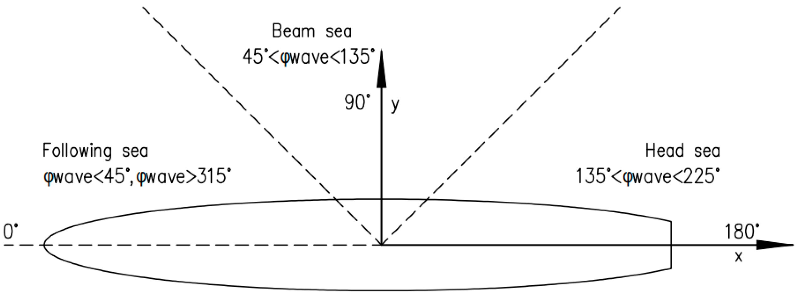The wave height is set to be the same in all four cases at 1.25 m, meeting the conditions outlined in Section 2.2 with the wave slope being less than 0.1412, and compatible with the frequencies mentioned above. The wave angle is set to 180 degrees in all four cases, representing the boat moving against the wave flow. The conditions are arbitrarily selected to evaluate the wave actuator’s performance. The tank coefficients are reiterated here for a more detailed description. Both the damping and spring coefficients are set to 20 in Cases 1, 2, and 3, while in Case 4, the damping coefficient is 25, and the spring coefficient is 40. They are tuned through trial and error. The boat’s initial velocity (Equation (11)) is 4.12 m/s for Case 4 and 2.06 m/s for the remaining three cases.

This paragraph introduces the types of simulation parameters and explains the reasons for their selection. In this study, the boat’s weight is fixed. Therefore, in Cases 1 and 4, the most influencing parameter affecting the force on the boat is the wave frequency (from 0.4 to 0.2 Hz), assuming that more wave crests will generate greater force on the wave actuator. The next influencing parameter is the boat’s initial velocity (2.06–4.12 m/s); the faster the boat, the more wave crests it encounters. Also, other important ones are the tank’s damping coefficient (from 20 to 25) and spring coefficient (from 20 to 40). These are the four parameters affecting the performance of the wave actuator. Considering the above, the following four simulation cases were conducted.

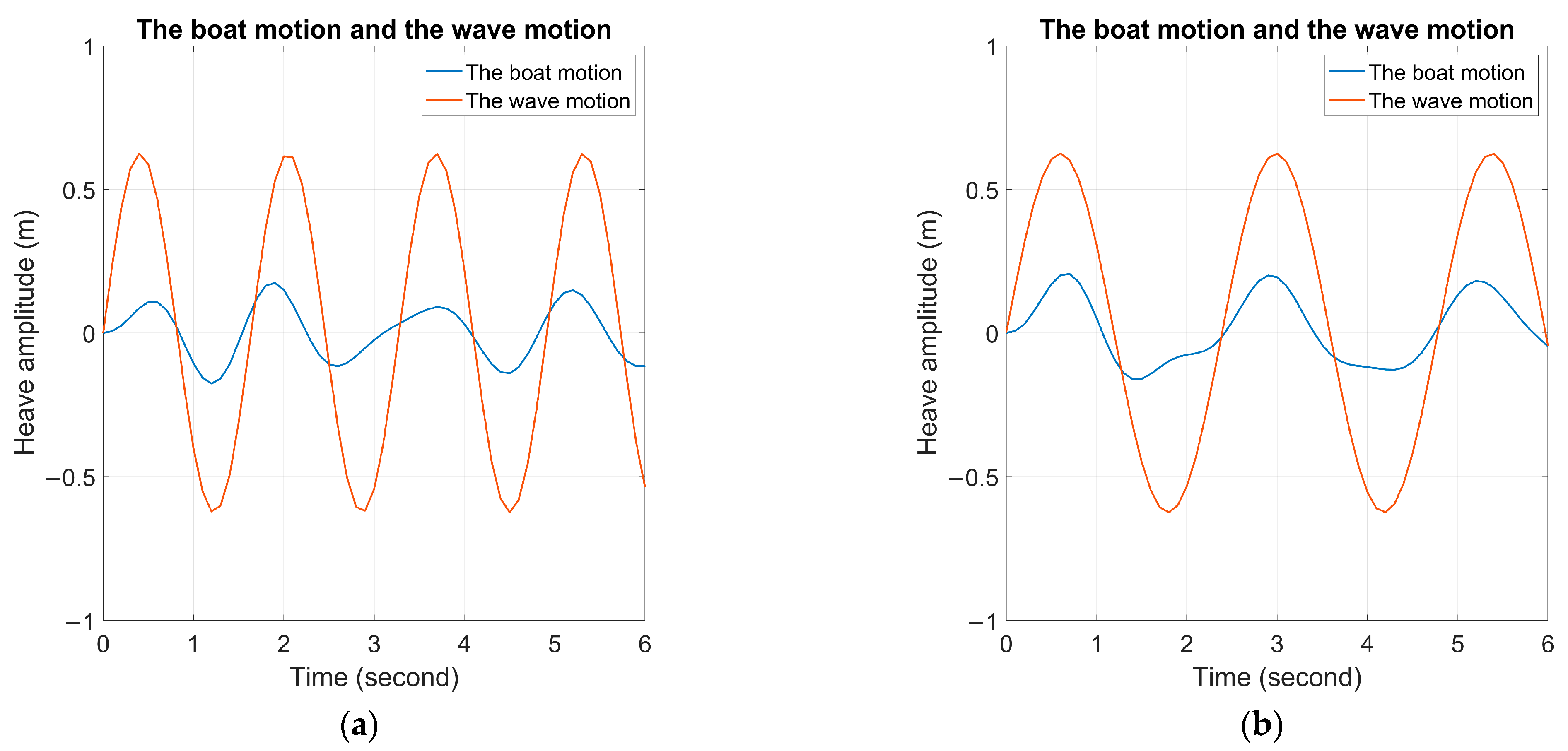
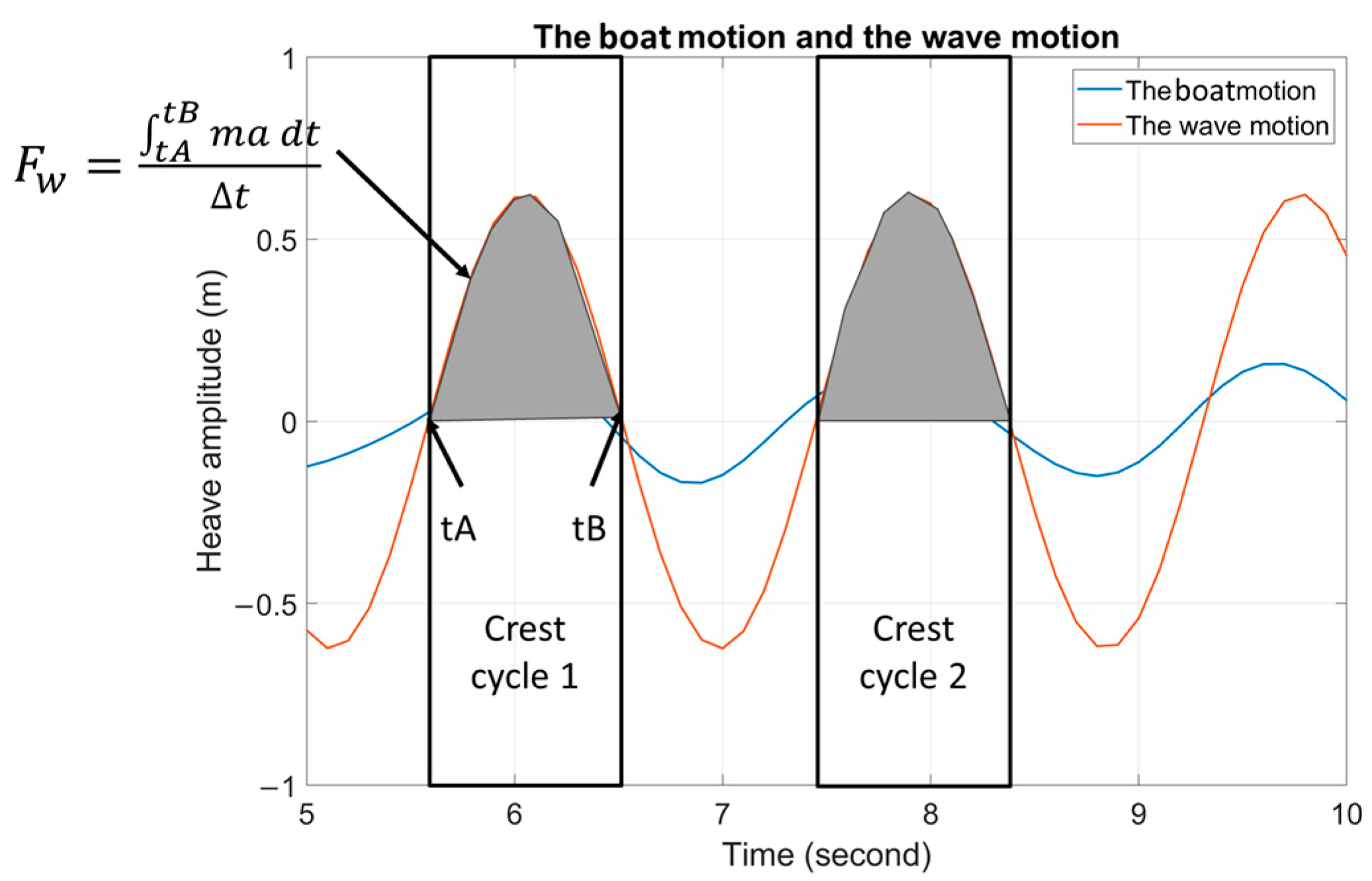
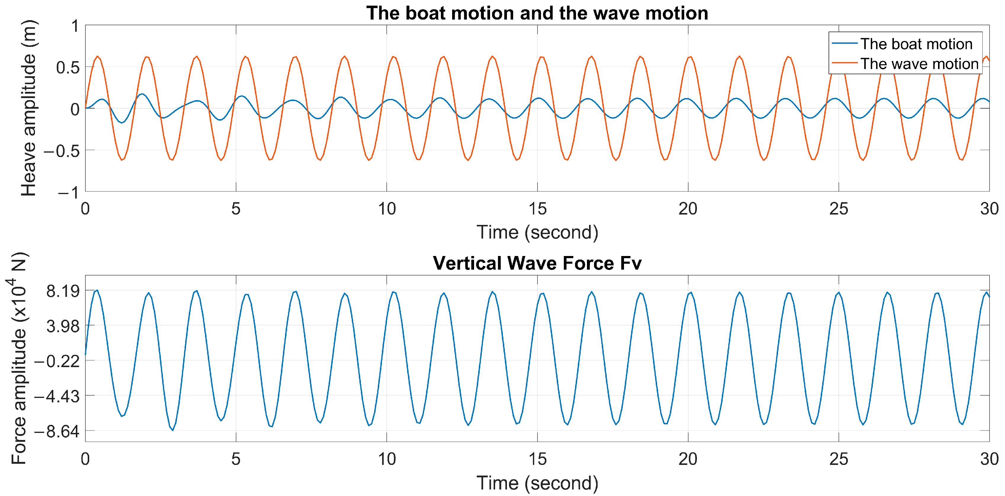
Before presenting the simulation results, here is a list of the information that will appear. In the graphs for all four cases, the orange line represents wave amplitude, and the blue line represents boat motion in the upper frame. Also, in all the vertical wave force figures, the lower frame shows the force amplitude, and the blue line represents the force over time acting on the wave actuator. These graphs assess the performance and behavior of the wave actuator under various wave conditions affecting the boat. The simulation results in all the tables in the four cases present the key information. The simulation parameters are reiterated, with the differences between the cases highlighted. The number of cycles refers to the upper half of the cycle shown in the amplitude graph. The calculated results for $P_c$ (Equation (31)), $P$ (Equation (30)), and $Mean{V}_{drag}$ (Equation (29)) are presented corresponding to each cycle. At the bottom of the table, the $Cruisespeed=1/M\sum _{i=1}^M{\left(Mean{V}_{drag}\right)}_i$, which represents the average speed achieved over 30 s of simulation. Here, $M$ denotes the total number of wave cycles considered in the simulation, and ${\left(Mean{V}_{drag}\right)}_i$ is the average velocity during the i-th wave cycle. The table also presents the corresponding efficiency values $\eta$ as defined in Equation (32). A time-domain simulation is conducted to evaluate the wave actuator’s performance under regular waves, while considering velocity and displacement constraints. The MATLAB code is employed to examine the interaction between the simulated boat motion and wave motion, as well as to analyze the wave force exerted on the boat over time.

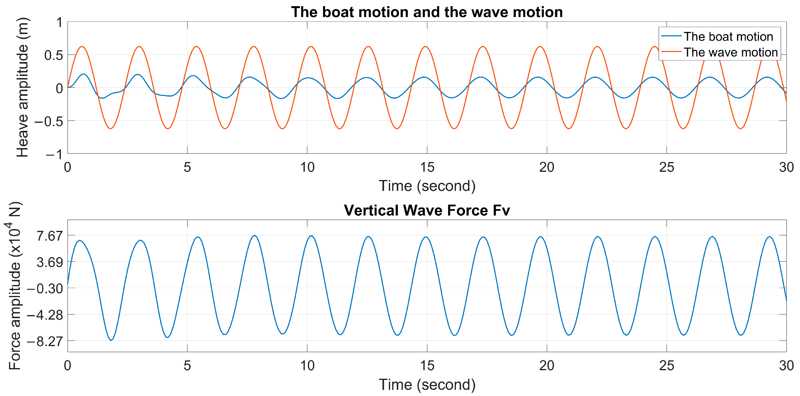
In Case 1, the boat had a damping coefficient of 20, a spring coefficient of 20, an initial speed of 2.06 m/s, and a wave angle of 180°. The simulation included displacement and velocity limits, suggesting that increasing wave amplitudes or draft size could improve wave energy conversion efficiency as depicted in Figure 11 and Table 3. A higher draft makes the boat more resistant to undulation, and changes to the boat’s initial velocity limit had little impact.

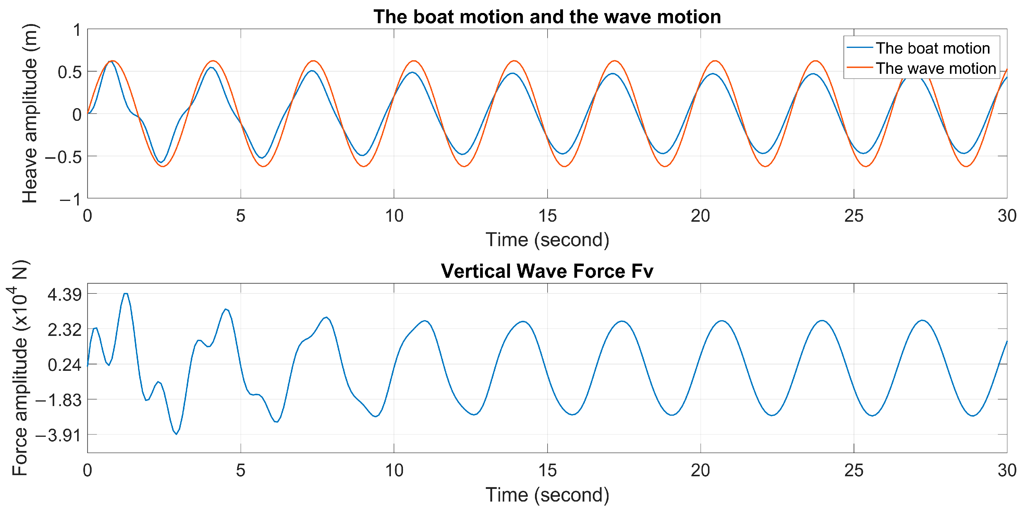
In Case 2, from Figure 12 and Table 4, it can be observed that the frequency for calculating the total force on the boat is adjusted, and similar to Case 3 (Table 5), reducing wave frequency decreased wave energy conversion. The simulation results for Case 4 did not fully meet expectations, as shown in Table 6. The simulation results for Case 4 did not fully meet expectations, as shown in Table 6.

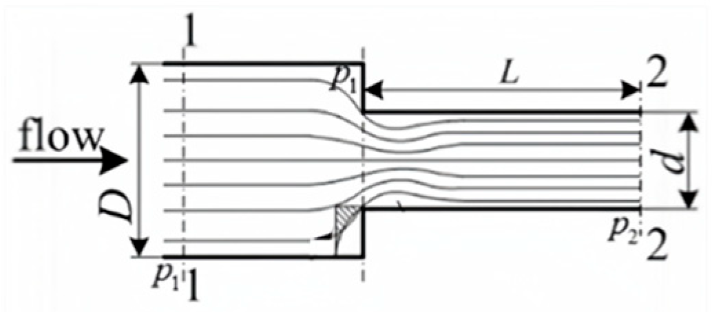
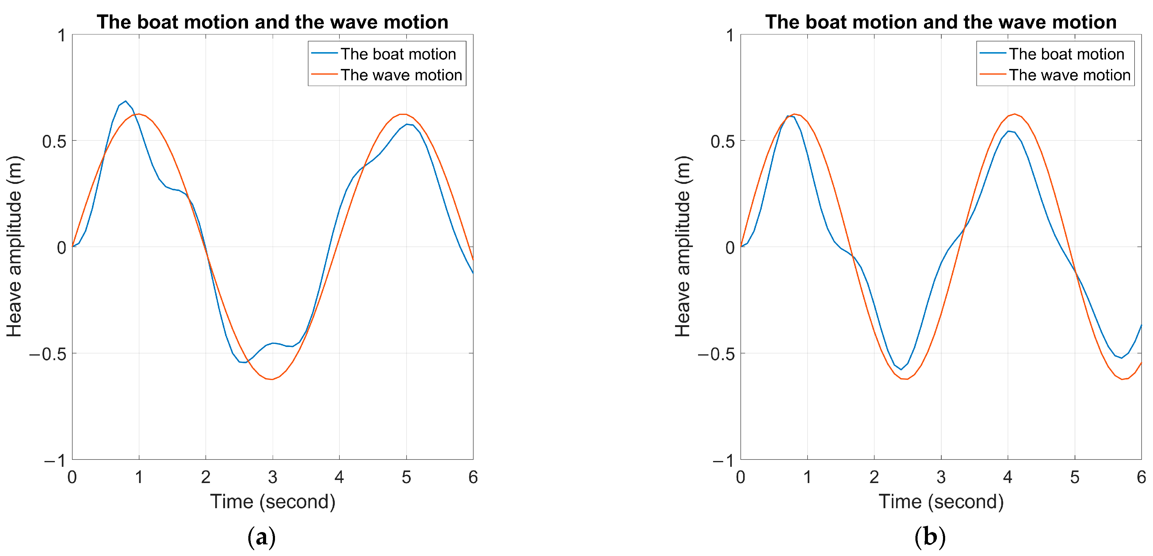
All waves have different speeds according to their wavelength. The wavelength ($wl$) is calculated using: $wl=g{T}^2/2\pi$, where $g=9.8\mathrm{m}/{\mathrm{s}}^2$ and $T$ is the wave period in seconds. Wavelength is inversely proportional to the frequency of the wave: waves with higher frequencies have shorter wavelengths, while waves with lower frequencies have longer wavelengths. Compared to Case 1, the wavelength in Cases 3 and 4 is much longer due to the reduced wave frequency. This is clearly illustrated in Figure 13 and Figure 14. The variation in boat motion and wave motion is not large, unlike Case 1.

In all cases, the oscillations of the waves and the boat both stabilized after about 5 s. As shown in Table 7 for comparison, Case 1 had a $Cruisespeed$ of 4.312 m/s and $\eta$ of 63.3% with wave angle of 180°. Case 2 had the highest $Cruisespeed$ of 6.098 m/s and $\eta$ of 67.9% with a frequency of 0.3 Hz, indicating good wave energy exploitation. Longer wave periods are expected to produce better results. However, in Case 3, $Cruisespeed$ and $\eta$ decreased significantly (4.768 m/s and 38.8%). Case 4 had a slight increase in $Cruisespeed$ and $\eta$ (5.233 m/s and 49.5%) due to changes in initial velocity and tank coefficients, but Case 2 was more efficient. Wave analysis and boat behavior are influenced by wave frequency and phase.

• Case 1

Figure 11. Amplitude graph for Case 1.

Figure 11. Amplitude graph for Case 1.

Table 3. Results of simulation for Case 1.

bt = 20.0; ct = 20.0; V = 4.0; Frequency = 0.4 Hz
	Cycle: 1	Cycle: 2	Cycle: 3	Cycle: 4	Cycle: 5	Cycle: 6
$P_c$ (W)	9621.81	17,842.5	24,538.2	33,914.2	39,691	48,778.2
$P$ (W)	83,259	87281	83,610.3	87,881.9	84,215.3	86,393.9
$Mean V_{drag}$ (m/s)	4.282	4.329	4.3	4.323	4.308	4.323
	Cycle: 7	Cycle: 8	Cycle: 9	Cycle: 10	Cycle: 11	Cycle: 12–15
$P_c$ (W)	54,813.3	64,200.2	69,229.9	76,613.4	81,309.9	85,393.9
$P$ (W)	84,992.1	87,717.9	86,426.4	88,394.4	90,070.8	94,692
$Mean V_{drag}$ (m/s)	4.311	4.313	4.312	4.316	4.315	4.316
$Cruise speed$: 4.312 m/s				$\eta$: 63.3%

Table 3. Results of simulation for Case 1.

bt = 20.0; ct = 20.0; V = 4.0; Frequency = 0.4 Hz
	Cycle: 1	Cycle: 2	Cycle: 3	Cycle: 4	Cycle: 5	Cycle: 6
$P_c$ (W)	9621.81	17,842.5	24,538.2	33,914.2	39,691	48,778.2
$P$ (W)	83,259	87281	83,610.3	87,881.9	84,215.3	86,393.9
$Mean V_{drag}$ (m/s)	4.282	4.329	4.3	4.323	4.308	4.323
	Cycle: 7	Cycle: 8	Cycle: 9	Cycle: 10	Cycle: 11	Cycle: 12–15
$P_c$ (W)	54,813.3	64,200.2	69,229.9	76,613.4	81,309.9	85,393.9
$P$ (W)	84,992.1	87,717.9	86,426.4	88,394.4	90,070.8	94,692
$Mean V_{drag}$ (m/s)	4.311	4.313	4.312	4.316	4.315	4.316
$Cruise speed$: 4.312 m/s				$\eta$: 63.3%

• Case 2

Figure 12. Amplitude graph for Case 2.

Figure 12. Amplitude graph for Case 2.

Table 4. Results of simulation for Case 2.

bt = 20.0; ct = 20.0; V = 4.0; Frequency = 0.3 Hz
	Cycle: 1	Cycle: 2	Cycle: 3	Cycle: 4	Cycle: 5
$P_c$ (W)	22,925.9	33,895.2	44,202.3	53,611.8	62,404
$P$ (W)	79,094.3	81,552.3	81,651.2	80,870.6	80,703
$Mean V_{drag}$ (m/s)	6.127	6.042	6.06	6.1	6.12
	Cycle: 6	Cycle: 7	Cycle: 8	Cycle: 9	Cycle: 10–11
$P_c$ (W)	71,576.6	78,523.3	80,348.3	80,355.8	80,335.9
$P$ (W)	82,948.6	86,387.9	94,915.6	105,155	115,362
$Mean V_{drag}$ (m/s)	6.115	6.107	6.102	6.102	6.103
$Cruisespeed$: 6.098 m/s				$\eta$: 67.9%

Table 4. Results of simulation for Case 2.

bt = 20.0; ct = 20.0; V = 4.0; Frequency = 0.3 Hz
	Cycle: 1	Cycle: 2	Cycle: 3	Cycle: 4	Cycle: 5
$P_c$ (W)	22,925.9	33,895.2	44,202.3	53,611.8	62,404
$P$ (W)	79,094.3	81,552.3	81,651.2	80,870.6	80,703
$Mean V_{drag}$ (m/s)	6.127	6.042	6.06	6.1	6.12
	Cycle: 6	Cycle: 7	Cycle: 8	Cycle: 9	Cycle: 10–11
$P_c$ (W)	71,576.6	78,523.3	80,348.3	80,355.8	80,335.9
$P$ (W)	82,948.6	86,387.9	94,915.6	105,155	115,362
$Mean V_{drag}$ (m/s)	6.115	6.107	6.102	6.102	6.103
$Cruisespeed$: 6.098 m/s				$\eta$: 67.9%

• Case 3

Figure 13. Amplitude graph for Case 3.

Figure 13. Amplitude graph for Case 3.

Table 5. Results of simulation for Case 3.

bt = 20.0; ct = 20.0; V = 4.0; Frequency = 0.2 Hz
	Cycle: 1	Cycle: 2	Cycle: 3
$P_c$ (W)	2923.52	4407.67	5248.25
$P$ (W)	16,700.1	16,544.7	14,413.7
$Mean V_{drag}$ (m/s)	4.787	4.7	4.822
	Cycle: 4	Cycle: 5	Cycle: 6
$P_c$ (W)	7055.82	8132.06	9455.58
$P$ (W)	15,930.3	15,679.1	16,583
$Mean V_{drag}$ (m/s)	4.76	4.771	4.768
$Cruise speed$: 4.768 m/s		$\eta$: 38.8%

Table 5. Results of simulation for Case 3.

bt = 20.0; ct = 20.0; V = 4.0; Frequency = 0.2 Hz
	Cycle: 1	Cycle: 2	Cycle: 3
$P_c$ (W)	2923.52	4407.67	5248.25
$P$ (W)	16,700.1	16,544.7	14,413.7
$Mean V_{drag}$ (m/s)	4.787	4.7	4.822
	Cycle: 4	Cycle: 5	Cycle: 6
$P_c$ (W)	7055.82	8132.06	9455.58
$P$ (W)	15,930.3	15,679.1	16,583
$Mean V_{drag}$ (m/s)	4.76	4.771	4.768
$Cruise speed$: 4.768 m/s		$\eta$: 38.8%

• Case 4

Figure 14. Amplitude graph for Case 4.

Figure 14. Amplitude graph for Case 4.

Table 6. Results of simulation for Case 4.

bt = 25.0; ct = 40.0; V = 8.0; Frequency = 0.2 Hz
	Cycle: 1	Cycle: 2	Cycle: 3	Cycle: 4
$P_c$ (W)	4542.35	7497.1	10,408.998	13,265.786
$P$ (W)	27,125.891	27,643.309	28,221.379	28,631.233
$Mean{V}_{drag}$ (m/s)	5.428	5.33	5.259	5.212
	Cycle: 5	Cycle: 6	Cycle: 7	Cycle: 8
$P_c$ (W)	16,118.897	18,764.279	21,223.052	23,432.669
$P$ (W)	29,268.216	29,821.467	30,550.743	31,532.541
$Mean{V}_{drag}$ (m/s)	5.183	5.163	5.144	5.141
$Cruisespeed$: 5.233 m/s			$\eta$: 49.5%

Table 6. Results of simulation for Case 4.

bt = 25.0; ct = 40.0; V = 8.0; Frequency = 0.2 Hz
	Cycle: 1	Cycle: 2	Cycle: 3	Cycle: 4
$P_c$ (W)	4542.35	7497.1	10,408.998	13,265.786
$P$ (W)	27,125.891	27,643.309	28,221.379	28,631.233
$Mean{V}_{drag}$ (m/s)	5.428	5.33	5.259	5.212
	Cycle: 5	Cycle: 6	Cycle: 7	Cycle: 8
$P_c$ (W)	16,118.897	18,764.279	21,223.052	23,432.669
$P$ (W)	29,268.216	29,821.467	30,550.743	31,532.541
$Mean{V}_{drag}$ (m/s)	5.183	5.163	5.144	5.141
$Cruisespeed$: 5.233 m/s			$\eta$: 49.5%

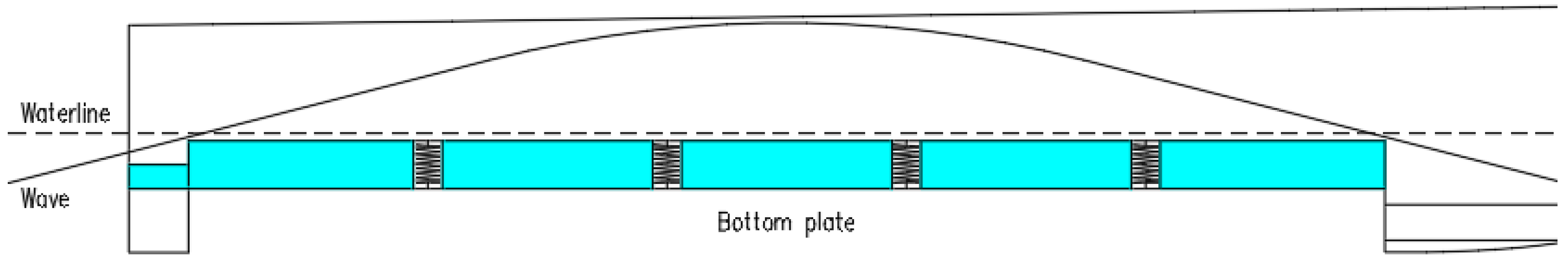
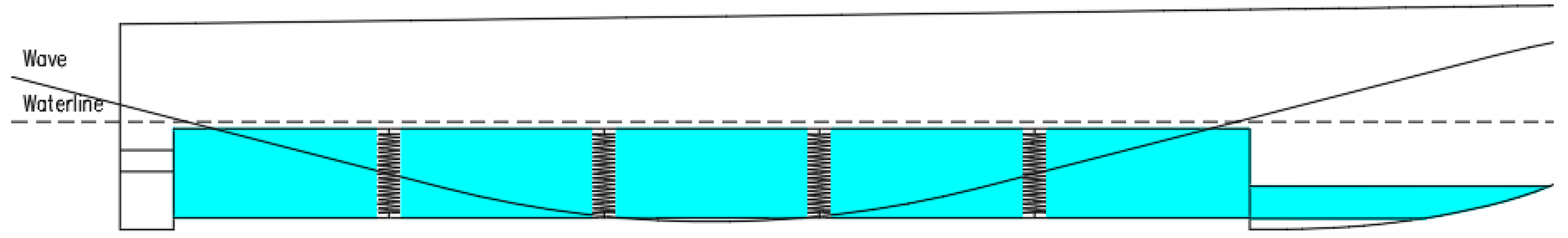
The wave energy conversion potential is highest in Case 2. Referring to Figure 5, the larger intersected area between the boat and wave motion implies more energy. In Case 1, the crests are too closely spaced due to high wave frequency, while Cases 3 and 4, the wavelengths are extended due to low wave frequency. Case 2 emerges as the optimal choice. In Case 2, the difference between the crest of the boat motion and the crest of the wave is the greatest, resulting in the highest pressure on the wave actuator out of the four cases.

Table 7. Simulation results.

	$\mathit{C}\mathit{r}\mathit{u}\mathit{i}\mathit{s}\mathit{e} \mathit{S}\mathit{p}\mathit{e}\mathit{e}\mathit{d}$ (m/s)	$\mathit{\eta }$ (%)
Case 1	4.312	63.3
Case 2	6.098	67.9
Case 3	4.768	38.8
Case 4	5.233	49.5

Table 7. Simulation results.

	$\mathit{C}\mathit{r}\mathit{u}\mathit{i}\mathit{s}\mathit{e} \mathit{S}\mathit{p}\mathit{e}\mathit{e}\mathit{d}$ (m/s)	$\mathit{\eta }$ (%)
Case 1	4.312	63.3
Case 2	6.098	67.9
Case 3	4.768	38.8
Case 4	5.233	49.5

Figure 15 and Figure 16 present the intersected area during the first 6 s of simulation for all four cases. Wave frequency is reduced from 0.4 to 0.2 Hz in all simulations. Tank coefficients and initial velocity are changed only in Case 4 to demonstrate the feasibility of increasing the input. As shown in Figure 15, the wave period has increased, allowing the system more time to convert wave energy. In Case 1, absorbed wave energy during one-cycle transition phase is smaller than in Case 2 ($P_c$ in Case 1 = 9621.806 W and $P_c$ in Case 2 = 22925.896 W). During the bullish wave phase, the area between the orange and blue lines is larger in Case 2 than Case 1.

To evaluate the prediction and simulation, we compare Cases 2 and 3, aiming to exploit the waves better with longer periods. Case 3 has a much larger wave period than Case 2, resulting in a smaller area between the orange and blue lines during the rising phase, as the boat moves with waves close to each other. The absorbed wave energy in Case 3 is converted in a shorter period ($P_c$ in Case 2 = 22925.896 W and $P_c$ in Case 3 = 2923.522 W). In 30 s of simulation, Case 2 has more cycles, resulting in a higher $\eta$ due to the wave crest applying more force on the tank bottom.

The absorbed wave energy at the transition phase of one cycle in Case 3 is smaller than in Case 4 ($P_c$ in Case 3 = 2923.522 W and $P_c$ in Case 4 = 4542.350 W). The increase in the tank coefficient has little effect on the final cruise speed result. However, doubling the boat’s initial speed from 2.06 m/s to 4.12 m/s, the cruising speed only increased from 4.8 m/s to 5.2 m/s, so this design parameter is not energy efficient.

4. Conclusions

A novel design for a wave actuator for boats is presented in this paper. The wave actuator is installed beneath the boat hull and converts the hydrodynamic forces generated by rising waves on the boat into translational thrusting forces. The compressed water in the tank of the wave actuator is expelled by the exerted wave pressure on the actuator, and the water thrust out of the nozzles propels the boat forward. The dynamics and hydrodynamics of the new wave actuator are presented using the second-order differential equation in this paper. Based on the modeling of the wave actuator, the analyses of the energy conversion capacity of the wave actuator are performed.

Computer simulations are performed to evaluate the performance of the new wave actuator for the boat. The simulations are carried out based on specific boat conditions and corresponding sea environments, as the following: the boat has a waterline length of 7.13 m, the waterline width is 2.26 m, the draft is 0.5 m, and the weight of boat displacement is 4397.9 kg. In four cases of simulation for regular waves, the wave frequency ranges are 0.4–0.2 Hz, the wavelength ranges are from 9.758 to 39.033 m, the wavenumber ranges are from 0.644 to 0.161, the wave height is 1.25 m, and the wave amplitude is 0.625 m. Of the four cases, the best result is observed in Case 2, where the wave frequency is 0.3 Hz, the water tank has a damping coefficient of 20, the spring coefficient is 20, and the boat speed is 2.06 m/s. Calculating the intersected area between the boat motion path and wave motion is significant. The 0.3 Hz frequency shows that the intersected area is the most suitable, avoiding the overly intense wave interactions that reduced conversion efficiency in Case 1, while also preventing the smallest area seen in the synchronized boat and wave motion in Case 3. Additionally, Case 4 is rejected because the low initial velocity means that the wave energy is purely converted into propulsion without the need for additional thrust from other engines. The most influential factors are wave frequency and initial velocity, which are clearly observed from the amplitude graph, where wave peaks clearly depict energy conversion capability.

In Case 2, the boat achieves a cruise speed of 6.098 m/s with 67.9% wave-to-propulsion efficiency. However, this warrants further analysis, as the design and equations were developed and simulated under idealized conditions. The intersected area suggests that the wave force acting on the boat is perfectly converted with no energy loss. The nozzle is assumed to achieve maximum efficiency, focusing only on the nozzle radius without describing the water flow path shape. Nonetheless, this high efficiency highlights the actuator’s potential for effectively harnessing wave energy for boat propulsion.

While this study presents a novel wave actuator system with promising theoretical performance, it is important to acknowledge its limitations. Due to the unique design of the actuator, there are no directly comparable systems or published results available for validation. Experimental data are currently unavailable, and the study relies on numerical simulations to demonstrate the feasibility of the concept. Our current work focuses on regular waves as an initial step to establish a clear theoretical foundation for the actuator’s dynamics and energy conversion capabilities. Future work will extend this analysis to more complex conditions and include experimental validation in a controlled environment, such as a wave tank, to confirm the practical applicability of the actuator. In particular, CFD simulations will be conducted to replicate fluid–structure interactions under realistic operating scenarios [28]. These simulations will refer to heave decay tests [29], as demonstrated in recent computational studies of floating sub-platforms, to better characterize hydrodynamic damping effects. Additionally, the model will be refined based on experimental findings to improve its accuracy and reliability. These steps will further strengthen the validity of the proposed system and pave the way for its real-world implementation.