Abstract
In order to solve the problems of low tracking accuracy of in-orbit satellites by ground stations and slow processing speed of satellite target tracking images, this paper proposes an orbital satellite regional tracking and prediction model based on graph convolutional networks (GCNs). By performing superpixel segmentation on the satellite tracking image information, we constructed an intra-frame superpixel seed graph node network, enabling the conversion of spatial optical image information into artificial-intelligence-based graph feature data. On this basis, we propose and build an in-orbit satellite region of interest prediction model, which effectively enhances the perception of in-orbit satellite feature information and can be used for in-orbit target prediction. This model, for the first time, combines intra-frame and inter-frame graph structures to improve the sensitivity of GCNs to the spatial feature information of in-orbit satellites. Finally, the model is trained and validated using real satellite target tracking image datasets, demonstrating the effectiveness of the proposed model.
1. Introduction
With continuous space activities, space situational awareness (SSA) has become a key research project in nations with space technologies, which can persistently track the non-space cooperation targets persistently by active laser detecting system in Earth stations [1,2]. In the space environments of low Earth orbit, the existing technologies for orbital correction in practice can effectively compensate the cumulative long-duration interferences on satellites from space perturbation forces, but the sudden disturbance caused by perturbation force will reduce the tracking precision of ground tracking systems [3,4]. Therefore, research on high-bandwidth instantaneous orbit perception and tracking correction techniques for the random orbital deviations of in-orbit satellites has become a central focus in SSA.
In order to improve the SSA performance of detecting systems, the current practice in astronomical observation institutions is to increase the optical antenna aperture of satellite–ground laser-detecting systems, which improves the echo detecting power for satellite targets. For example, the McDonald Observatory in Texas, USA, employed a telescope with an optical aperture of 0.76 m [5]; the Zimmerwald Observatory in Switzerland constructed a telescope with an optical aperture of 1.2 m [6]; the optical ground station of the European Space Agency in Tenerife, Spain, was equipped with a telescope that has an optical aperture of 1 m [7]; the Zi Jinshan Observatory in Shanghai, China, is equipped with a telescope whose optical aperture is 1.5 m [8]. Changchun Observatory of the National Astronomical Observatories uses a telescope with an optical aperture of 1 m [9]. However, referring to the theories of classical applied optics, when simply increasing the aperture of the optical antenna, the focal length will increase in the optical systems, thereby reducing the detecting field of view. Therefore, while improving the aperture of the optical antenna, imaging detectors with larger imaging surface size (such as CCD CMOS) should be adopted to maintain the range of the detecting field of view [10]. Benefiting from the development of semiconductor imaging detectors, imaging detector products with large image surface sizes have been gradually enriched. The method that realizes high robust target sensing and tracking by combining the large-aperture optical antenna with the large-image surface size imaging detector has become a development trend to improve the SSA capability of on-orbit targets [11]. However, further increasing the size of imaging detectors results in a nonlinear growth of tracking image data; hence, the image data processing capability of the existing tracking systems cannot meet the real-time technical requirements.
In recent years, methods achieving highly robust target tracking by deep learning on spatiotemporal context information have been proposed [12,13,14]. The Convolutional Long Short-Term Memory (ConvLSTM) network combined the spatial awareness of convolutional neural networks with the temporal memory characteristics of LSTM, effectively modeling dynamic changes in image sequences. It was particularly suitable for spatiotemporal data modeling tasks [15]. However, its complex architecture and large number of parameters resulted in high training costs, and it suffered from the vanishing gradient problem when processing long sequences.The 3D Convolutional Neural Network (3D-CNN) captured variations across both temporal and spatial dimensions using three-dimensional convolution, offering a compact structure and high inference efficiency [16]. It was well suited for short-term motion prediction tasks. Nonetheless, its inherent fixed time window limited its adaptability to variable-length sequence prediction, and its modeling capacity was constrained in long-term prediction tasks. U-Net Recurrent Prediction integrated the classic encoder–decoder structure of U-Net with a temporal recurrence mechanism to achieve target prediction [17]. It offered advantages such as a lightweight model, ease of training, and deployment, making it suitable for resource-constrained environments. However, due to the lack of explicit temporal sequence modeling, this method had certain limitations in capturing target motion trends. Optical Flow explicitly modeled displacement information of targets through the optical flow field, offering strong physical interpretability and being well suited for rigid targets or static background scenarios [18]. However, the performance of this method was highly dependent on the quality of optical flow estimation, and its prediction accuracy degraded significantly in the presence of occlusion, complex deformation, or low-contrast regions. Pix2Pix GAN, as a type of conditional generative adversarial network, performed well in preserving image structure and edge details, generating high-quality images [19]. It was particularly suitable for scenarios requiring high visual fidelity. However, the GAN training process itself was relatively unstable, and the generated results were sensitive to training strategies and loss function weight settings.
Compared with the aforementioned traditional spatiotemporal modeling methods, graph convolutional networks (GCNs) demonstrated unique advantages in modeling target motion trends. Unlike convolution-based models such as ConvLSTM and 3D-CNN, which relied on fixed grid structures, GCNs naturally adapted to non-Euclidean data structures, making them particularly suitable for dynamic graph structures constructed from centroid trajectories extracted from sequential mask images. This graph-based representation explicitly modeled inter-frame structural dependencies, effectively enhancing the model’s ability to capture temporal continuity of the target. Furthermore, spatiotemporal graph convolutional networks (ST-GCNs), by decoupling temporal and spatial modeling, exhibited stronger performance in modeling long-term dependencies compared to U-Net recurrent structures. In contrast to optical flow methods—which could only handle apparent motion between two frames and lacked predictive capability—GCNs enabled future trend prediction based on multiframe graph structures, expanding both the depth and foresight of modeling. Compared with generative adversarial networks such as Pix2Pix GAN, GCNs did not rely on pixel-level aligned data, and could effectively model using sparse yet robust graph structures (e.g., centroids or edge features), thereby reducing computational overhead and enhancing generalization. More importantly, GCNs offered strong model interpretability: their explicit adjacency relationships intuitively reflected inter-frame motion linkages, while also supporting multimodal feature fusion at the node level (e.g., velocity, category, optical flow), granting high extensibility and flexibility. As a result, GCN-based methods for target prediction and tracking had attracted increasing attention [20,21,22].
Although existing GCN methods had been widely applied in areas such as action recognition, multiobject tracking, and traffic prediction, direct application to LEO satellite imagery targets acquired from ground stations posed adaptation challenges. Satellite images typically had low frame rates, small targets, and blurry edges, while GCNs required robust graph structures and were prone to underfitting. Due to the high speed of satellite target movement and large inter-frame displacements, GCNs—being sensitive to “node locality”—often suffered from collapsed graph connectivity and unstable training.
To address these challenges, we proposed a novel Intra-Inter Graph Convolutional Network (I²-GCN) for tracking LEO satellite targets. This framework simultaneously learned intra-frame and inter-frame graph structures to systematically capture the spatiotemporal evolution of the target. By integrating both intra-frame and inter-frame graph features, the proposed model effectively improved tracking robustness and communication efficiency. In other words, this study introduced a new predictive tracking method at the algorithmic level, which contributed to resolving control-related issues and provided valuable insights for the future development of space-air target tracking systems. In other words, a new tracking target prediction method at the algorithm level was applied to improve the problem in the control field, providing a reference for the future development of space and space target tracking system.
In order to verify the feasibility of this method, continuous tracking experiments on space targets was conducted at the Changchun Observatory of the National Astronomical Observatory Chinese Academy of Sciences (CAS) and real space target tracking image data was acquired to build a dataset.
2. Related Work
2.1. The Acquisition of Raw Data
Relying on the Changchun Artificial Satellite Observation Station of the National Astronomical Observatories, Chinese Academy of Sciences, we conducted a series of continuous acquisition and tracking experiments for the Starlette satellite, which operates in an orbit with an altitude of approximately 813–821 km and an orbital period of about 105 min [23]. As a low Earth orbit (LEO) satellite, Starlette was probably affected by different perturbations such as the non-spherical gravity from the Earth, tides, three-body perturbation, solar radiation pressure, and atmospheric drag on its orbit resulting in long-term accumulation errors and short-term random errors [24]. At present, the long-term accumulated error of the track prediction system through the ground station has been calibrated, but the short-term random error still presents a challenge to the robustness of the tracking system.
As shown in Figure 1, the on-orbit target tracking system of the ground station was composed of track forecasting system, laser transmitting system, echo receiving system, servo control system, and computer processing system. The laser transmitting system was equipped with a nanosecond laser whose wavelength and power were, respectively, 532 nm, 30 W as the transmitting source and a refracting optical antenna with a diameter of 20 cm. The receiving system adopted an optical antenna with aperture of 1 m, and the optical signal received by the optical antenna was divided into two beams through the spectroscope, which were, respectively, received by the single photon detector and the low-light-level camera. The control system was driven by independent azimuth and pitch direct drive motors with a maximum rotation rate of 5 degrees/s. The pointing accuracy was 1 arcsec, and the pointing accuracy after stellar calibration was about 5 arcsec.
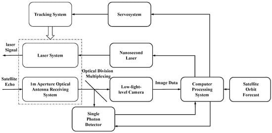
Figure 1.
Satellite tracking system diagram.
Firstly, with the telescope guided by the ground station tracking the satellite according to the satellite forecast, a directional high-energy laser beam was emitted into space by the laser emitting system, which was reflected back to the ground station by the angle reflector of the satellite as the echo light signal. Then, through the 1 m aperture optical antenna, the echo light signal was effectively focused on the photosurface of the low-light-level camera. The tracking image data of the satellite target was obtained after the above process.
The original image data of the on-orbit target continuous tracking image was integrated to construct a dataset. Specifically, the original image data consisted of more than 3000 images, among which 1000 continuous tracking image data of different time periods were selected as the dataset (some images were shown in Figure 2). The dataset covers a variety of features in the actual satellite target tracking, including target acquisition, target deviation, target miss, and so on. We used 500 consecutive images as the training set to train the I²-GCN predictive tracking model, and another 500 images as the test set for model validation.
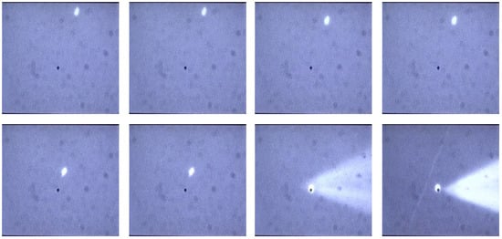
Figure 2.
Satellite target image.
2.2. Elaboration of Problems
During the missions of on-orbit target tracking observation at Earth stations, on the one hand, the time window in which the target satellite is observed is limited to less than 10 min because of the zenith angle and observational environments. If the target satellite misses, the time window is wasted for recapture. The mentioned situation indicated that on-orbit target tracking systems required higher robustness. On the other hand, the echo signals only occupied an extremely small portion of the detection target surface in a large detector, and a large amount of computing resources were wasted in repetition of collecting, transmitting and processing redundant information, which seriously affected the improvement in the bandwidth of the tracking system. Therefore, there is a great engineering significance in developing a tracking algorithm with high robustness and high bandwidth for the target tracking mission of on-orbit satellites.
3. Model Structure
In this paper, we propose an orbital satellite region tracking prediction model based on graph convolutional networks (GCNs). Figure 3 illustrates the overall framework of the proposed model. The model consists of four parts: preprocessing of satellite target video frames, construction of intra-frame and inter-frame graph structures (Section 3.1 and Section 3.2), spatiotemporal prediction model for spatial targets (Section 3.3), and the model training module.
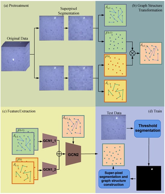
Figure 3.
I²-GCN Overall framework of model.
During the preprocessing stage, we use the Simple Linear Iterative Clustering (SLIC) method to perform superpixel segmentation on two consecutive frames of the images. In the graph structure construction stage, we use the superpixel seeds from the segmentation as graph nodes. The intra-frame graph structure (intra-frame adjacency matrix) is established based on the principle that adjacent nodes are connected. Then, the inter-frame graph structure (inter-frame adjacency matrix) is constructed by connecting all superpixel nodes that exceed the segmentation threshold between two frames.
Next, we built a feature extraction model composed of two layers of graph convolutions. The first layer consists of two sets of graph convolution structures, taking the tracking target features and the intra-frame adjacency matrix as inputs. The second layer accepts the concatenated results of the two sets of GCN outputs from the first layer and the inter-frame adjacency matrix as input, ultimately outputting the predicted superpixel node features, which are then reconstructed into an image.
During model training, we treat the video frames from the third frame onward as the control group. The threshold segmentation results of the control group images are used for superpixel segmentation, with the pixel values of the superpixel seeds serving as the expected output of the model, used to train the proposed GCN model.
3.1. Data Preprocessing
To enable prediction of the target’s positional region, it was necessary to extract the target areas from the dataset. We applied the SLIC superpixel segmentation method to perform superpixel processing on the original image data [25]. In this method, K-means clustering was used for center sampling and the image was segmented into different pixel blocks with the cluster center as the seed point. The superpixel replaced the original pixel level data, which significantly reduced the computational amount of the subsequent processing [26]. Through the superpixel segmentation method, the region of interest (ROI) of the tracked target was marked. Meanwhile, for subsequent visualization analysis, we retained the feature matrix of each pixel block and the positional information of each superpixel block. The superpixel segmentation result S could be expressed as follows:
where n was the number of superpixel blocks after image segmentation, () was the superpixel segmentation function, U was the original image data, was the superpixel graph of a single image, and N was the nth superpixel obtained by applying function () to the segmentation of U. To ensure that the output size of the model matched the original size, it was necessary to store the relevant information in . Therefore, could be expressed as follows:
where n was the index of the superpixel block, was the average brightness value of the pixels in the nth superpixel block, and was the set of positions of all the pixels that made up the nth superpixel block. The SLIC method used in this paper performed superpixel segmentation of the satellite target’s continuous tracking image data at multiple scales. To better validate the model’s performance, five scales were used for superpixel segmentation of the target image, namely, . Some of the results of the superpixel segmentation are shown in Figure 4.
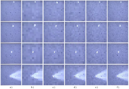
Figure 4.
The results of different scale superpixel segmentation: (a) Raw image; (b) The result of superpixel segmentation scale 100; (c) The result of superpixel segmentation scale 196; (d) The result of superpixel segmentation scale 256; (e) The result of superpixel segmentation scale 324; (f) The result of superpixel segmentation scale 1024.
3.2. Construct Graph Structure
3.2.1. Construct Intra-Frame Graph Structure
Research shows that models based on planar convolutions, such as CNN, RNN, and LSTM, could be applied to target detection tasks. However, directly processing images as primary data when extracting spatial and temporal features increased the overall computational load of the model. Moreover, the large number of parameters posed significant challenges to the storage space of some terminal devices. Therefore, when the input data volume was large or when the system had strong real-time requirements, the computational time overhead was significantly increased. As a result, we adopted the lower computational cost approach of graph convolution to build the target tracking model. We used the superpixel segmentation results to construct the graph structure for the tracked target, with the superpixel seeds serving as the nodes of the graph. We constructed the graph structure for each frame in the target tracking video in the same manner. The process could be expressed as follows:
where was the graph structure computed for the mth frame of video I, represented the superpixel segmentation result of the mth frame of the target tracking video, () was the graph structure construction function, and M was the total number of frames in the target tracking video.The graph structure consisted of the adjacency matrix, degree matrix, and feature matrix, and could be expressed in the following form:
where A represented the adjacency matrix between the intra-frame nodes, and its calculation process could be expressed as follows:
Here, indicated that superpixel block was spatially adjacent to superpixel block , and, correspondingly, indicated that the two superpixel blocks were not spatially adjacent. D was the degree matrix of the nodes, and its calculation process could be expressed as follows:
was the feature matrix of the graph nodes in the mth frame. We used the average brightness of all superpixel blocks in the mth frame as the threshold, and constructed the feature matrix using the binarized segmentation result. Its calculation process could be expressed as follows:
was obtained using Equation (3), while was independently calculated for each frame and remained fixed within that frame. This statistical approach ensured that the inter-frame adjacency criteria were consistent, data-dependent, and repeatable across the entire dataset.
At this point, we had completed the construction of the intra-frame graph structure. In the first layer of the proposed model, we used a graph convolutional network in combination with the intra-frame graph structure to calculate the regions of the target within the frame. The specific computation process of the model was detailed in Section 3.3. The superpixel segmentation method was used to convert the original image data into graph structure data. This data type not only captured the spatial relationships of the tracked target but also contained the inherent features of the image data, while also reducing the computational overhead.
3.2.2. Construct Inter-Frame Adjacency Matrix
In target tracking tasks, methods that utilize the temporal sequence of image sequences to assist in tracking the target have been widely applied. For example, the inter-frame differencing method and the inter-frame differencing multiplication method were used to improve the tracking target detection accuracy by extracting and processing inter-frame information from the sequence of images. On the other hand, context-based algorithms utilized the changing patterns of the target object’s shape and motion attributes over time to complete the target tracking task. This approach is mainly suitable for application scenarios that required high tracking accuracy and robustness. Graph convolutional networks could aggregate the neighbor information of nodes and extract the features of those nodes. In the previous section, we constructed the intra-frame adjacency matrix for the tracked target using superpixel blocks as nodes, thus extracting the spatial features of the tracked target. However, in addition to identifying the current spatial position of the target object, the model also needed to predict the possible future spatial positions of the target object. Therefore, it was necessary to use a graph structure to represent the relationship of the target object’s motion direction across consecutive frames. To distinguish it from the previously introduced concept of the “intra-frame adjacency matrix”, we referred to the adjacency matrix that describes the target object’s motion direction information as the “inter-frame adjacency matrix”. The corresponding graph structure was called the “inter-frame graph structure”. Therefore, based on the definition of the graph structure, the inter-frame graph structure could be expressed as follows:
where represented the inter-frame graph structure composed of the superpixels from the th frame and the tth frame image, and was the inter-frame adjacency matrix that constituted . Its calculation process could be expressed as follows:
where was the ith superpixel block in the th frame, was the jth superpixel block in the tth frame, and the connection criterion between and could be expressed as follows:
Here, and , respectively, represented the average brightness of all superpixels in the th frame and the tth frame. As shown in Equations (14) and (15), if the brightness of the nth superpixel block in the th frame was greater than the average brightness of that frame, and the brightness of the ith and jth superpixel blocks in the tth frame was also greater than the average brightness of that frame, then the elements in the ith and jth columns of the nth row of the inter-frame adjacency matrix were assigned a value of 1.
represented the inter-frame degree matrix composed of the superpixels from the th frame and the tth frame image. could be obtained from , and its calculation process is referred to in Equation (8).
represented the inter-frame feature matrix between the th and tth frames. Unlike the calculation method of the intra-frame feature matrix, the inter-frame feature matrix was not directly expressed by the intra-frame superpixel information. Instead, it was the result of applying graph feature extraction to the graph structures of the adjacent two frames, followed by a concatenation operation. It could be expressed as follows:
Here, and were the first part of the graph feature extraction functions in the model, and we would detail this section in Section 3.3.
3.3. Construct Spatiotemporal Prediction Model
We designed an orbital satellite region tracking prediction model composed of two parts using graph convolutional networks. In the first part of the model, we designed two graph neural networks, each with two layers of graph convolutions. Accordingly, we input the intra-frame graph structure data of two adjacent frames into each graph neural network with two layers of graph convolutions, then concatenated the two output results to obtain the final output of the first part of the network. Thus, the feature extraction process of one of the graph neural networks in the first part could be expressed as follows:
where W was the graph convolution kernel. was the graph convolution function, and could be expressed as follows:
where ,, I was the identity matrix, and F was the feature matrix, as shown in Equation (10).
The second part of the model consisted of a two-layer graph convolutional network, and the computation process is referred to in Equations (17)–(19). Unlike the previous section, we used the inter-frame graph structure as the input to the second part of the model, as described in Section 3.2.2. The detailed structure of the model that predicted the third frame based on information from two consecutive frames is shown in Table 1.

Table 1.
The specific structure of the model.
3.4. Visualization of Graph Features
In our GCN-ROI prediction and tracking model, the prediction features of the output target ROI could be fed back to the control system for closed-loop tracking.
In our model, the predicted target region of interest features were output and could be fed back to the control system for closed-loop tracking. To demonstrate the prediction results and facilitate subsequent result analysis, we combined the superpixel information to restore the model’s output position prediction vectors into images. We refer to this process as “visualization of graph features”. Algorithm 1 shows the pseudocode for the process of visualizing graph features. We constructed a function called preamention to process each set of data.
| Algorithm 1: Visualization of graph features. |
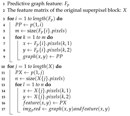 |
4. Experimental Results and Analysis
The dataset used in this study was constructed based on continuous satellite target tracking image data acquired from the Changchun Artificial Satellite Observation Station of the National Astronomical Observatories, Chinese Academy of Sciences. The dataset consisted of 1000 consecutive satellite tracking images, all resized to a resolution of 256 × 256. A total of 50% of the dataset was used as the training set, and the remaining 50% was used as the test set. In this section, we quantitatively and qualitatively evaluate the performance of the proposed model.
4.1. Train
As graph neural networks (GCNs) rely on the topological structure of graphs to propagate information, different superpixel scales directly determine the “graph resolution” and the “complexity of the adjacency graph”, thereby affecting the model’s representation capacity and convergence. Therefore, we conducted a comprehensive ablation study. First, we transformed the training set—composed of real satellite target tracking images—into graph structures using five different segmentation scales: 100, 196, 256, 324, and 1024, and saved the corresponding superpixel information. Then, we applied the algorithm described in Section 3.2 to compute the inter-frame adjacency matrices for all the graph-structured data. Finally, we input the graph structure data and inter-frame adjacency matrices into our designed multilayer graph convolutional neural network for deep learning.
In addition, as the GCN model proposed in this study follows a supervised learning framework, the region-of-interest labels required during the training phase were generated heuristically. Specifically, we first performed binary mask processing on each frame of the image. In the resulting mask images, the foreground target regions appeared as bright areas (white), while the background remained black. Next, the images were segmented into multiple superpixel regions based on brightness thresholds. Superpixels with brightness values higher than the average were identified as target regions and used to construct the training labels. The dimension of each training label was N × 1.
To evaluate the accuracy of the automatically generated labels, we randomly selected 100 image–mask pairs from the training set for manual inspection. The review was conducted by two researchers familiar with image preprocessing and superpixel segmentation. The results showed that over 95% of the samples were highly consistent with the expected target regions. Approximately 5% of the samples exhibited minor errors such as boundary deviation or multitarget interference. To maintain automation and reproducibility in the labeling process, these samples were retained for training.
For the test set, in order to ensure the objectivity and accuracy of model evaluation, manually annotated mask images were used as ground-truth labels. The manual annotation process involved pixel-level delineation of the target regions by trained researchers, producing high-quality “gold standard” labels. All performance evaluation metrics reported in this paper(such as IoU, Dice, SSIM, and RMSE) were calculated based on these manually annotated labels in the test set.
Considering the stochastic nature of the algorithm, we trained multiple I²-GCN prediction models using different numbers of epochs: 50, 100, 200, 500, and 1000. The mean squared error (MSE) was adopted as the loss function, with Adam as the optimizer and a learning rate of 0.001. Our model was validated on a validation set consisting of 500 real satellite target tracking images. The visualized output of the validation set is shown in Figure 5, where we used a difference heatmap to compare the predicted images with the ground-truth mask images.
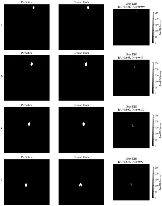
Figure 5.
Visual comparison between predicted target masks and ground truth annotations for four representative test samples. For each case (a–d), the left column shows the predicted binary mask, the middle column shows the corresponding ground truth, and the right column shows the pixel-wise difference (Gray Diff) along with the calculated Intersection over Union (IoU) and Dice coefficient. These examples demonstrate the model’s prediction accuracy under different target sizes and locations.
4.2. Model Evaluation and Predictive Assessment
Structure similarity (SSIM) [27] and correlation coefficient (CC) [28] were chosen to evaluate the proposed model. SSIM measures the overall similarity of two images by comparing their correlation in brightness, contrast, and structure.
where t was the true image data of the tracking target, p was the image data predicted by the model, and , , , , and were the statistics of t and p, which represented mean, variance, and covariance. and were area constants which were 0.01 and 0.03, respectively.
CC measured the correlation between two sets of data by calculating the cosine of the angle between them in their sample space. It was defined as follows:
where and were the standard deviations of the graph features predicted by the model and the real target graph features, respectively. The use of a joint evaluation method based on SSIM and CC could comprehensively assess the model’s performance in terms of structural preservation and pixel-level consistency, helping to identify different types of distortions and improving the accuracy of the evaluation.
Then, to assess the accuracy and fit of the predicted model results from different perspectives, root mean squared error (RMSE) [29] and R-square (R²) [30] were used for joint evaluation. RMSE is an indicator that measures the average difference between the predicted values and the actual values. It was obtained by calculating the average deviation of corresponding pixels between the original image data and the visualized graph feature image data processed in Section 3.4. The calculation formula was
where m and n were the height and width of the image, and and represented the pixel values at position in the original and predicted images, respectively. R² was used to assess the strength of the relationship between the predicted values and the actual values. It was obtained by calculating the ratio of the residual sum of squares to the total sum of squares between the images. The calculation formula was
where was the average value of all the pixels in image . In satellite image target prediction and tracking, RMSE could quantify the model’s prediction error, while R² reflected the model’s ability to explain the changes in the target’s position. By combining both, a more comprehensive evaluation of the model’s performance could be achieved.
Finally, to quantitatively evaluate the region overlap accuracy between the predicted images and the ground-truth masks, we adopted two classical metrics: intersection over union (IoU) and the Dice coefficient. IoU measures the ratio between the intersection and the union of the predicted and ground-truth regions. It is mathematically defined as
Here, P denoted the predicted image output by the model, and T denoted the image data from the validation set. Compared to IoU, the Dice coefficient (also known as a variant of the F1-score) placed greater emphasis on the relative proportion of the intersection area. It was defined as
In this study, the two metrics were used as complementary indicators to comprehensively characterize the model’s performance in region localization and boundary reconstruction.
4.3. Analysis of Experimental Results
The hardware system used in our experiments was DDR4 2666 MHz 16 GB memory, and the software environment included Python 3.9, GPU version of PyTorch 2.5, and CUDA 11.8.
4.3.1. Ablation Study
We obtained multiple trained models using different superpixel scales and epochs. To validate the effectiveness of the proposed tracking compensation method, we conducted a series of ablation experiments.
First, we used the SSIM and CC metrics from Section 4.2 to evaluate all the models.
In Figure 6a, the results of comparing the structural similarity between the predicted images generated by models with different superpixel scales and epoch settings and the test set images are presented. From these comparisons, it could be observed that as the superpixel scale increased, the structural similarity between the predicted and test images generally showed an upward trend. However, this trend was neither linear nor absolute. For instance, under a superpixel scale of 324, the outputs from models trained with different epochs did not significantly outperform those obtained at a superpixel scale of 256 in terms of structural similarity. This indicated that, under certain conditions, increasing the superpixel scale did not always lead to improvements in structural similarity, which might also be affected by model training stability and other factors.
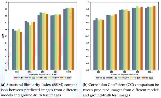
Figure 6.
Quantitative evaluation of prediction results using SSIM (a) and CC (b) metrics.
As shown in the linear correlation coefficient comparison results in Figure 6b, the correlation coefficient between the predicted images and the test set images generally increased with higher superpixel scales. However, for models with superpixel scales of 256, 324, and 1024, the growth trend of the correlation coefficient was relatively flat.
Additionally, for both SSIM and CC metrics, performance under the same superpixel scale tended to stabilize as the number of training epochs increased.
To further evaluate the impact of superpixel scale on the performance of the I²-GCN model, we recorded the MSE loss convergence curves during training under different superpixel scales (100, 196, 256, 324, and 1024), as illustrated in Figure 7. Among these, the model with a superpixel scale of 324 achieved the lowest final MSE loss and exhibited the smoothest convergence curve, indicating excellent prediction stability. In contrast, the model with a superpixel scale of 1024 maintained a relatively high loss throughout the training process, which may have resulted from over-segmentation leading to sparse graph structures, or the limited capacity of the graph neural network to model complex spatial relationships.
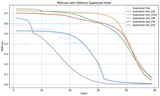
Figure 7.
The MSE loss of models trained with different superpixel scales (100, 196, 256, 324, and 1024).
These findings indicated that a moderate number of superpixels (e.g., 256–324) could achieve an effective balance between spatial resolution and modeling stability, thereby enhancing the performance of I²-GCN in target prediction and tracking tasks.
Finally, this study evaluated the model’s prediction error using root mean squared error (RMSE) and R-squared (R²) metrics under different superpixel scales. As shown in the Figure 8, with increasing superpixel scale, RMSE exhibited a downward trend, while R² continued to rise. When the number of superpixels was 100 and 196, the model struggled to capture local dynamic details due to the coarse segmentation, resulting in high RMSE and low R². As the number increased to 256 and 324, the model performance improved significantly, with RMSE decreasing to a lower level and R² rising above 0.8. Notably, at a superpixel scale of 1024, R² reached its highest value, indicating that the model almost completely captured the target’s changing trend. However, RMSE showed a slight increase, suggesting that over-segmentation may introduce noise or detail interference.

Figure 8.
Comparison of RMSE and R² for models under different superpixel scales.
To validate the effectiveness of the I²-GCN model in satellite target prediction and tracking tasks, we conducted a comparative study with existing state-of-the-art methods. These models included ConvLSTM (based on CNNs), 3D-CNN (utilizing three-dimensional convolutional networks), U-Net (with a fully symmetric architecture), Pix2Pix (based on conditional GAN), and the Farneback optical flow method combined with SimpleUNet. To adapt these models for satellite target prediction and tracking, we made necessary modifications. All models were trained using the labeled satellite target tracking image dataset constructed in this study, with the number of training epochs set to 50.
We evaluated all models using the six metrics defined in Section 4.2. Table 2 presents the quantitative comparison between our method and the five baseline approaches. The results show that the proposed I²-GCN model performed excellently across all six metrics. In particular, the RMSE dropped to 7.92—the lowest among all models—while the R² reached 0.8649, indicating the strongest explanatory power of the predicted output with respect to the variations in the ground-truth images.
Table 2.
Performance comparison of different experimental methods.
4.3.2. Overhead Time
In the space target tracking missions, the overall efficiency was determined by the bandwidth of tracking systems. Therefore, in this section, the time overhead of the model was analyzed.
We tested the impact of different segmentation scales and epoch settings on the time cost of the model, as shown in Table 3. It was observed that higher segmentation precision led to increased time cost, with a significant rise when the superpixel scale reached 1024. In contrast, under the same segmentation scale, the variation in the number of epochs did not result in significant changes in time consumption.
Table 3.
Time cost under different segmentation scales and epochs (ms).
The proposed I²-GCN model directly processed the graph-structured data generated from superpixel segmentation, resulting in very low computational cost. According to measurements of floating point operations per second (FLOPS), the model required only 1.59 MFLOPS. However, it should be noted that the superpixel segmentation process required for graph construction introduced some computational overhead.
In practical applications, the superpixel segmentation process could be integrated into CMOS imaging modules equipped with FPGA hardware, enabling direct output of graph-structured data through hardware acceleration and avoiding the loss of computational resources. Additionally, the visualization and feature fusion processes were primarily intended for experimental analysis. In real-world deployment, the spatial target features could be directly fed back to the tracking system as compensation, without consuming bandwidth.
Experimental results demonstrated that the proposed I²-GCN-based target prediction and tracking method achieved both high computational efficiency and accuracy. Nonetheless, although increasing segmentation precision improved prediction accuracy, it also significantly increased the time cost. Therefore, in practical applications such as prediction–tracking–compensation systems, different prediction models should be selected based on actual requirements and resource constraints.
5. Conclusions and Future Work
This paper applied the GCN algorithm to the task of orbital satellite region tracking and prediction. For the first time, a combination of intra-frame and inter-frame graph structures was used, allowing the graph convolutional network to perform spatiotemporal prediction tasks. This approach solved the issue of reduced computational efficiency in target tracking models based on CNN networks due to data redundancy.
The proposed algorithm was tested at the Changchun Observatory of the National Astronomical Observatory, Chinese Academy of Sciences, and the impact of different superpixel segmentation scales on the performance of the proposed model was verified. The results showed that the model significantly improved both the tracking accuracy and bandwidth. Our algorithm not only increased the data processing speed but also significantly improved the bandwidth and tracking accuracy of the tracking system.
The orbital satellite region tracking model proposed in this paper provides an efficient and robust solution for satellite target tracking, but there is still room for further research and optimization. For example, during the process of constructing graph structure data, we only used the SLIC method. In the future, more efficient and accurate superpixel segmentation methods could be explored to further reduce computational costs. Similarly, in terms of model construction, increasing the depth of graph convolution layers could be considered to capture more complex spatiotemporal features, thereby improving tracking accuracy.
In the future, we will also incorporate tracking data for satellites with different orbits and types, expand the training dataset, and improve the model’s generalization capability.
Author Contributions
Conceptualization, S.W. and Y.M.; methodology, S.W.; software, R.W.; validation, Y.J.; formal analysis, X.D.; investigation, M.I.; resources, Y.M.; data curation, G.W.; writing—original draft preparation, S.W.; writing—review and editing, X.D.; visualization, M.I. and J.L.; supervision, Y.M.; project administration, X.D.; funding acquisition, Y.M. All authors have read and agreed to the published version of the manuscript.
Funding
This research was funded by the Natural Science Foundation Project of Jilin Province (20240101300JC).
Institutional Review Board Statement
Not applicable.
Informed Consent Statement
Not applicable.
Data Availability Statement
The dataset used in this study is subject to a confidentiality agreement and cannot be shared. However, the core model architecture and training configuration files are available at: https://github.com/ws874694232/I2-GCN-architecture (accessed on 2 June 2025).
Conflicts of Interest
The authors declare no conflicts of interest.
References
- Cohen, G.; Afshar, S.; Morreale, B.; Bessell, T.; Wabnitz, A.; Rutten, M.; van Schaik, A. Event-based Sensing for Space Situational Awareness. J. Astronaut. Sci. 2019, 66, 125–141. [Google Scholar] [CrossRef]
- Verspieren, Q. The United States Department of Defense space situational awareness sharing program: Origins, development and drive towards transparency. J. Space Saf. Eng. 2020, 8, 86–92. [Google Scholar] [CrossRef]
- Li, J.; Yang, Z.; Luo, Y. Intention inference for space targets using deep convolutional neural network. Adv. Space Res. 2025, 75, 2184–2200. [Google Scholar] [CrossRef]
- Kumar, R.; Singh, R.; Chinnappan, A.K.; Appar, A. Simulation of the orbital decay of a spacecraft in low Earth orbit due to aerodynamic drag. Aeronaut. J. 2022, 126, 565–583. [Google Scholar] [CrossRef]
- Wilkinson, M.; Schreiber, U.; Prochazka, I.; Moore, C.; Degnan, J.; Kirchner, G.; Zhongping, Z.; Dunn, P.; Shargorodskiy, V.; Sadovnikov, M.; et al. The next generation of satellite laser ranging systems. J. Geod. 2019, 93, 2227–2247. [Google Scholar] [CrossRef]
- Rodriguez-Villamizar, J.; Cordelli, E.; Schildknecht, T. The stare and chase observation strategy at the Swiss Optical Ground Station and Geodynamics Observatory Zimmerwald: From concept to implementation. Acta Astronaut. 2021, 189, 352–367. [Google Scholar] [CrossRef]
- Rattenbury, N.J.; Ashby, J.; Bennet, F.; Birch, M.; Cater, J.E.; Ferguson, K.; Giggenbach, D.; Grant, K.; Knopp, A.; Knopp, M.; et al. Update on the german and australasian optical ground station networks. Int. J. Satell. Commun. Netw. 2025, 43, 147–163. [Google Scholar] [CrossRef]
- Wu, Z.; Zhang, H.; Deng, H.; Long, M.; Cheng, Z.; Zhang, Z.; Meng, W. The progress of laser ranging technology at Shanghai Astronomical Observatory. Geod. Geodyn. 2019, 10, 492–498. [Google Scholar] [CrossRef]
- Liang, Z.; Dong, X.; Ibrahim, M.; Song, Q.; Han, X.; Liu, C.; Zhang, H.; Zhao, G. Tracking the space debris from the Changchun Observatory. Astrophys. Space Sci. 2019, 364, 201. [Google Scholar] [CrossRef]
- Li, K.; Wan, G.; Cheng, G.; Meng, L.; Han, J. Object detection in optical remote sensing images: A survey and a new benchmark. Isprs J. Photogramm. Remote Sens. 2020, 159, 296–307. [Google Scholar] [CrossRef]
- Zhang, H.; Liu, H.; Xu, W.; Lu, Z. Large aperture diffractive optical telescope: A review. Opt. Laser Technol. 2020, 130, 106356. [Google Scholar] [CrossRef]
- Zhang, K.; Zhang, L.; Liu, Q.; Zhang, D.; Yang, M.H. Fast Visual Tracking via Dense Spatio-Temporal Context Learning; Springer International Publishing: Berlin/Heidelberg, Germany, 2014. [Google Scholar] [CrossRef]
- Yuan, D.; Chang, X.; Li, Z.; He, Z. Learning Adaptive Spatial-Temporal Context-Aware Correlation Filters for UAV Tracking. Acm Trans. Multimed. Comput. Commun. Appl. 2022, 18, 1–18. [Google Scholar] [CrossRef]
- Li, J.; Wang, J.; Liu, W. Moving Target Detection and Tracking Algorithm Based on Context Information. IEEE Access 2019, 7, 70966–70974. [Google Scholar] [CrossRef]
- Kim, J.; Choo, H.; Jeong, J. Self-Attention (SA)-ConvLSTM Encoder-Decoder Structure-Based Video Prediction for Dynamic Motion Estimation. Appl. Sci. 2024, 14, 11315. [Google Scholar] [CrossRef]
- Liu, Y.; Wang, C.; Xu, S.; Zhou, W.; Chen, Y. Multi-weighted graph 3D convolution network for traffic prediction. Neural Comput. Appl. 2023, 35, 15221–15237. [Google Scholar] [CrossRef]
- Zhang, Z.; Xue, W.; Liu, Q.; Zhang, K.; Chen, S. Learnable Diffusion-Based Amplitude Feature Augmentation for Object Tracking in Intelligent Vehicles. IEEE Trans. Intell. Veh. 2024, 9, 4749–4758. [Google Scholar] [CrossRef]
- Sormoli, M.A.; Dianati, M.; Mozaffari, S.; Woodman, R. Optical Flow Based Detection and Tracking of Moving Objects for Autonomous Vehicles. IEEE Trans. Intell. Transp. Syst. 2024, 25, 12578–12590. [Google Scholar] [CrossRef]
- Zhao, X.; Yu, H.; Bian, H. Image to Image Translation Based on Differential Image Pix2Pix Model. CMC-Comput. Mater. Contin. 2023, 77, 181–198. [Google Scholar] [CrossRef]
- Zhang, Y.; Zheng, L.; Huang, Q. Multi-object tracking based on graph neural networks. Multimed. Syst. 2025, 31, 89–101. [Google Scholar] [CrossRef]
- Su, M.; Ni, P.; Pei, H.; Kou, X.; Xu, G. Graph Feature Representation for Shadow-Assisted Moving Target Tracking in Video SAR. IEEE Geosci. Remote Sens. Lett. 2025, 22, 4004905. [Google Scholar] [CrossRef]
- Wei, L.; Zhu, R.; Hu, Z.; Xi, Z. UAT:Unsupervised object tracking based on graph attention information embedding. J. Vis. Commun. Image Represent. 2024, 104, 104283. [Google Scholar] [CrossRef]
- Lejba, P.; Schillak, S. Determination of station positions and velocities from laser ranging observations to Ajisai, Starlette and Stella satellites. Adv. Space Res. 2011, 47, 654–662. [Google Scholar] [CrossRef]
- Zou, K.; Hao, Z.; Feng, Y.; Meng, Y.; Hu, N.; Steinhauer, S.; Gyger, S.; Zwiller, V.; Hu, X. Fractal superconducting nanowire single-photon detectors working in dual bands and their applications in free-space and underwater hybrid LIDAR. Opt. Lett. 2023, 48, 415–418. [Google Scholar] [CrossRef]
- Achanta, R.; Shaji, A.; Smith, K.; Lucchi, A.; Fua, P.; Suesstrunk, S. SLIC Superpixels Compared to State-of-the-Art Superpixel Methods. IEEE Trans. Pattern Anal. Mach. Intell. 2012, 34, 2274–2281. [Google Scholar] [CrossRef] [PubMed]
- Prakash, J.; Kumar, B.V. An Extensive Survey on Superpixel Segmentation: A Research Perspective. Arch. Comput. Methods Eng. 2023, 30, 3749–3767. [Google Scholar] [CrossRef]
- Bakurov, I.; Buzzelli, M.; Schettini, R.; Castelli, M.; Vanneschi, L. Structural similarity index (SSIM) revisited: A data-driven approach. Expert Syst. Appl. 2022, 189, 116087. [Google Scholar] [CrossRef]
- Humphreys, R.K.; Puth, M.T.; Neuhaeuser, M.; Ruxton, G.D. Underestimation of Pearson’s product moment correlation statistic. Oecologia 2019, 189, 1–7. [Google Scholar] [CrossRef]
- Khalid, S.; Goldenberg, M.; Grantcharov, T.; Taati, B.; Rudzicz, F. Evaluation of Deep Learning Models for Identifying Surgical Actions and Measuring Performance. JAMA Netw. Open 2020, 3, e201664. [Google Scholar] [CrossRef]
- Rights, J.D.; Sterba, S.K. R-squared Measures for Multilevel Models with Three or More Levels. Multivar. Behav. Res. 2023, 58, 340–367. [Google Scholar] [CrossRef]
Disclaimer/Publisher’s Note: The statements, opinions and data contained in all publications are solely those of the individual author(s) and contributor(s) and not of MDPI and/or the editor(s). MDPI and/or the editor(s) disclaim responsibility for any injury to people or property resulting from any ideas, methods, instructions or products referred to in the content. |
© 2025 by the authors. Licensee MDPI, Basel, Switzerland. This article is an open access article distributed under the terms and conditions of the Creative Commons Attribution (CC BY) license (https://creativecommons.org/licenses/by/4.0/).