Abstract
Seismic signal processing often relies on general convolutional neural network (CNN)-based models, which typically focus on features in the time domain while neglecting frequency characteristics. Moreover, down-sampling operations in these models tend to cause the loss of critical high-frequency details. To this end, we propose a feedback information distillation network (FID-N) in the non-subsampled contourlet transform (NSCT) domain to remarkably suppress seismic noise. The method aims to enhance denoising performance by preserving the fine-grained details and frequency characteristics of seismic data. The FID-N mainly consists of a two-path information distillation block used in a recurrent manner to form a feedback mechanism, carrying an output to correct previous states, which fully exploits competitive features from seismic signals and effectively realizes the signal restoration step by step across time. Additionally, the NSCT has an excellent high-frequency response and powerful curve and surface description capabilities. We suggest converting the noise suppression problem into NSCT coefficient prediction, which maintains more detailed high-frequency information and promotes the FID-N to further suppress noise. Extensive experiments on both synthetic and real seismic datasets demonstrated that our method significantly outperformed the SOTA methods, particularly in scenarios with low signal-to-noise ratios and in recovering high-frequency components.
1. Introduction
Oil and gas resources are not only the cornerstone of social and economic development but also the guarantee of national security. With the construction of the national digital detection network, the observation methods and technologies of the new Internet of Things are gradually being applied, which basically realizes the digitization, networking, and integration of seismic monitoring and exploration, and the ability to carry out seismic monitoring and exploration has been greatly improved. The application of digital technology provides rich first-hand data for seismic scientific research and lays a good foundation for explanations and predictions of seismic exploration. Noise attenuation is crucial to obtain high-quality data from the seismic signals that are collected with geophone sensing equipment and networks. But these are usually badly interfered with and distorted by noises in seismic exploration. This has an important impact on oil and gas exploration. Therefore, this paper aimed to obtain high-quality seismic data to delicately portray the subsurface geological structure and make a more reliable geological interpretation.
While acquiring seismic data, the reflected seismic signals are recorded together with incoherent noise by geophones. These noises seriously interfere with real seismic data and produce distortion in seismic exploration. Therefore, noise suppression remains a pivotal step for obtaining high-quality seismic signals that can reliably inform oil and gas exploration decisions. Currently, many algorithms for seismic noise suppression, e.g., the first seismic denoising approach [1], denoising approaches based on the transform domain [2,3,4] and sparse transform [5,6,7,8], learning-based approaches [9,10], and other types of methods [11,12,13,14], have been developed. In fact, random noise, which is the most common seismic noise, can penetrate the whole time domain, severely distorting and interfering with real seismic data. Since the seminal random noise suppression method introduced by Canales [1], multiple refinements and alternative techniques have emerged, including empirical mode decomposition (EMD)-based approaches, sparse transform-based approaches, variational mode decomposition techniques, and fast dictionary learning-based approaches [10]. Chen and Ma [4] proposed an f-x empirical mode decomposition-based algorithm, where the random noise is removed by using predictive filtering. Chen and Fomel [6] presented a new EMD-seislet transform-based algorithm for removing the random noise from seismic data. Liu et al. [7] reported a variational mode decomposition approach to suppress seismic random noise. In fact, a widely used and effective method of seismic random noise suppression algorithms is based on the multi-scale geometric analysis sparse transform. Zhang et al. [2] built a wavelet transform-based denoising algorithm with an improved seismic data resolution. Neelamani et al. reported a curvelet transform-based random noise attenuation method [3], and various subsequent variants [8,12] also achieved satisfactory results. Lin [14] suggested a seismic random noise suppression method based on the decomposition performed by three-dimensional (3D) steerable pyramids. Notably, Genovese et al. [15] extended the potential of wavelet analysis in seismic applications by employing circular harmonic wavelets for the generation and analysis of non-stationary ground motions.
With the increasing use of current social intelligence, more and more fields are introducing artificial intelligence and deep learning (DL) algorithms [16,17,18,19,20,21,22,23,24,25,26] to solve related problems, including seismic denoising. Zhang et al. [27] implemented the automatic identification and localization of geological faults based on machine learning and deep learning methods, respectively. Cao et al. [28] used a modified depth confidence network to identify carbonates from logging data and also used the network to process seismic data to obtain additional information. Huang et al. [29] designed a big data platform that combined convolutional neural networks and different machine learning models to increase the recognition accuracy of faults. Olivier et al. [30] reported a sparse weighting-based matrix decomposition method to use supervised machine learning to separate active interference signals from coherent background noise sources. Jia et al. [31] proposed an intelligent Monte Carlo machine learning method based on support vector regression for the intelligent interpolation processing of seismic data. Zhang et al. [32] designed a U-Net deep neural network model for denoising seismic data, with good denoising results. Mai et al. [33] proposed a deep residual seismic denoising model, which overcomes the limitation of the number of network layers in deep learning algorithms. Compared with previous shallow neural networks, the seismic signal features are learned more adequately, and the noise suppression is better. Fang et al. [34] presented a CNN with a dual residual structure, which allows arbitrary combinations between two operators of different layer pairing operations to extract richer features and helps improve denoising performance. Yu [35] made improvements to a DnCNN by using a form of null convolution in its convolution kernel to increase the field of perception of seismic data, which can both efficiently denoise and protect the effective signal. In order to attenuate seismic random noise, Sang et al. [36] constructed a novel unconventional algorithm based on a proximal classifier with consistency (PCC) in the transform domain. To simultaneously suppress coherent and incoherent seismic noises, this group suggested another deep neural network-based seismic denoising approach [37,38]. The group suggested that it is feasible to draw on its emerging disciplinary field approach to address relevant problems in the geophysical domain. Moreover, Liu et al. [26] proposed an unsupervised learning method that utilizes end-to-end convolutional neural networks for seismic image denoising, aiming to learn the features of effective signals and suppress unpredictable random noise. Li et al. [39] simulated synthesized images with different resolutions and noise levels as the training set and combined the L1 loss and the multi-scale structural similarity loss to improve the perceptual quality of the original data. Chang et al. [40] employed Fourier domain adaptation to achieve domain transfer. First, they replaced the amplitude spectrum of synthetic seismic data with the amplitude spectrum of real seismic data for feature space mapping. Then, the network model was transferred and trained using synthetic seismic data to improve its performance on real seismic data. Min et al. [41] proposed a dual-encoder U-Net to exploit the details and edge information of data, using a main decoder for high-resolution recovery and an edge decoder for edge contour monitoring with the aim of improving the resolution of noisy seismic data and maintaining data fidelity.
The DL models mentioned earlier are applied in many different scenarios for seismic data reconstruction, including synthetic and field datasets. However, most of them only consider the seismic features in the time domain when training the DL models, which ignores the frequency information of seismic data, i.e., the multi-scale features of seismic data. Additionally, the prevalent use of pooling operations within CNN-based models, intended to expand receptive fields, often inadvertently compromises the detailed seismic reflection features, adversely affecting the data reconstruction accuracy. For the above challenges, this paper proposes a new DL-based denoising algorithm in the non-subsampled contourlet transform (NSCT) domain to effectively suppress seismic noise, particularly for seismic data with a low signal-to-noise ratio (SNR). This network avoids building models and assumptions because a huge training set is used for training, raw data are employed as inputs, and the desired clean data are the corresponding outputs. The present work has the following contributions:
- (1)
- This paper proposes a new feedback information distillation network (FID-N) that mainly consists of a two-path information distillation (ID) block used in a recurrent manner to form a feedback mechanism, with the advantage of sharing the weights of each iterative block during the procedure, and fully exploits features from seismic signals and effectively restores the noisy seismic signals step by step.
- (2)
- Noise suppression is formulated to predict the NSCT coefficients to further remove noise with the FID-N while preserving more details compared with spatial-domain algorithms.
- (3)
- Our scheme was verified with synthetic and real seismic data and demonstrated both qualitatively and quantitatively that the denoised data obtained with our method had higher SNR values and richer useful information compared with those obtained with other cutting-edge methods, especially for high-frequency low-SNR data.
2. Related Work
Seismic data acquisition, essential for oil and gas exploration, often faces the challenge of noise interference. The most common form of seismic noise is random noise, which can penetrate the entire time domain and significantly distort real seismic data. Over the years, numerous noise suppression techniques have been developed to mitigate such interference and enhance seismic data quality.
Traditional methods, such as transform-domain-based approaches and sparse transforms, have been widely used for seismic denoising. Some early work by Canales [1] introduced a random noise suppression technique, which was further refined with methods like empirical mode decomposition (EMD) [4], wavelet transforms [2], and curvelet transforms [3]. These techniques have demonstrated their ability to suppress random noise, but they often struggle with more complex, non-stationary noise types.
More recent advancements in seismic denoising have leveraged machine learning and deep learning (DL) techniques. Several studies have explored the use of DL for seismic signal restoration. For example, Zhang et al. [32] proposed a U-Net deep neural network for seismic data denoising, achieving significant improvements in noise removal. Similarly, Mai et al. [33] introduced a deep residual seismic denoising model, which surpassed traditional shallow neural networks in learning seismic features and reducing noise. Other work, such as that by Fang et al. [34], utilized CNNs with dual residual structures to improve feature extraction and denoising performance. Li et al. [42] used the self-attention mechanism in the moving window to effectively suppress random seismic noise based on the Swin Transformer model in 2D seismic data denoising, thus improving the signal-to-noise ratio.
Despite the success of these methods, many existing approaches still focus predominantly on the time-domain features of seismic signals, neglecting frequency-domain information. This oversight often leads to suboptimal performance, particularly when dealing with seismic data characterized by low signal-to-noise ratios (SNRs). To address this, recent research has emphasized the importance of multi-scale feature extraction and the incorporation of frequency-domain information. For example, Liu et al. [26] developed an unsupervised learning method for seismic image denoising using convolutional neural networks, while Chang et al. [40] proposed a Fourier-domain adaptation technique to enhance the performance of seismic models on real data. Chen et al. [43] used the Swin Transformer and a multi-scale channel attention enhancement U-Net to improve seismic denoising, addressing complex noise in synthetic and in situ seismic data. Zhang et al. [44] used an adaptive time–frequency denoising method to solve source-related seismic noise, dynamically optimizing the threshold curve to effectively suppress high-amplitude noise and improve signal recovery.
This paper builds upon these advancements by proposing a novel feedback information distillation network (FID-N) that operates in the NSCT domain. This method aims to effectively suppress seismic noise, especially in low-SNR conditions, by utilizing a two-path information distillation block in a recurrent manner. The feedback mechanism in the FID-N allows for iterative denoising, leveraging the strengths of each stage to improve the data quality progressively.
3. Proposed Method
Firstly, the structure of our FID-N will be described. Secondly, the designed two-path ID block will be briefly introduced, and lastly, the NSCT domain prediction will be proposed.
3.1. Architecture for FID-N Seismic Denoising Network
As shown in Figure 1, the proposed FID-N has two modules: a signal shallow feature extraction (SSFE) module and a feedback module that has iterativeness and corrects the input of the system by rerouting the output in each loop. The feedback module contains a two-path information distillation module (IDB) that can distill more useful information based on collecting as much information as possible. The FID-N can be unfolded as a set of temporally ordered iterations ranked from 1 to T. T represents the number of iterations over which the FID-N unfolds and processes temporal information in a sequence.
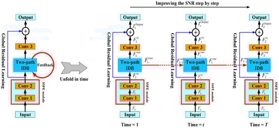
Figure 1.
Architectural diagram of our FID-N network. Red and blue arrows denote the feedback and global residual skip connections, respectively.
Inspired by [45], our proposed network is optimized with L1 loss. Given the noisy seismic signals and clean seismic signals , the FID-N loss function is given by
where denotes a weight factor that quantifies the importance or relevance of the output generated in the t-th iteration in the context of the iterative process. This factor can be used to adjust the influence of the t-th iteration’s output on the subsequent computations or final results. represents the parameter of the FID-N. Following [45], = 1 for each iteration, representing that the contribution of each output is equal.
Specifically, double convolution layers (“Layer-1” and “Layer-2”, respectively) are utilized to perform SSFE on noisy seismic signals. The first layer captures the initial features, and the second layer refines them, improving feature extraction. The extracted shallow feature in the t-th iteration is calculated by
where and are convolution operations of Layer-1 and Layer-2, respectively. The shallow features are then used as the input to the two-path IDB.
In the two-path IDB, the hidden state of the previous iteration is fed back to the t-th iteration and the shallow features . represents the output of the two-path IDB:
where represents the operation of our proposed two-path IDB as well as the actual feedback process. More details of the two-path IDB can be found in Section 3.2. Integrally, to obtain the feature maps in the t-th iteration, global residual learning is used in this work, which can be formulated as
where and H3 denotes the convolution operation of ‘Conv 3’ in Figure 2.
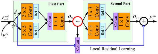
Figure 2.
Two-path information distillation block (IDB).
Each convolutional layer in our FID-N has 64 filters. This paper obtains, in total, T denoised seismic data after T iterations.
In Figure 1, the SSFE module consists of two convolutional layers with 3 × 3 and 5 × 5 convolutional kernels, with a stride of 1. Conv 3 is the convolutional layer with 3 × 3 convolutional kernels. Table 1 shows the SSFE structure.

Table 1.
Structure of signal shallow feature extraction.
3.2. Two-Path Information Distillation Block (IDB)
Figure 2 shows the designed two-path IDB that consists of two parts to take advantage of short- and long-path features, respectively. This two-path network differs from the information distillation network (IDN) model because it is constructed in every part and different paths use different convolutional kernels. Therefore, our algorithm can adaptively measure the features of the short and long paths at different scales.
As shown in Figure 2, the inputs of the first part in the t-th iteration are and . This paper obtains the following fusion:
where denotes the concatenation of and . is a 1 × 1 convolutional layer composite function. So, the output of the first part is
where denotes the ReLU function [46]; , , and are the functions of 1 × 1, 3 × 3, and 5 × 5 convolutional layers in , respectively; and stands for the concatenation of the feature maps by various convolutional kernels. Then, the concatenation of the 64-dimensional (64D) feature maps of and the input are conducted in the channel dimension as Equation (7):
where S represents the slicing operation. As shown in Figure 2, except for the feature fusion layer, which employs 128 filters, all other convolutional layers are designed with 64 filters. Thus, we extract 64-dimensional feature maps from the 128-dimensional features generated by feature fusion. By combining the current 64-dimensional features with the previous , this process can be viewed as retaining short-path (SP) information. Subsequently, the remaining 64-dimensional features are used as the input for the second part to extract long-path (LP) information:
where , , and are the functions of 1 × 1, 3 × 3, and 5 × 5 convolutional layers in the second part, respectively. In the last, this paper expresses the aggregation of the input information, the SP information, and LP information by
For the 1 × 1 convolution kernel, it is only 1 × 1 in size, so it does not need to consider the relationship between pixels and surrounding pixels. It is mainly used to adjust the number of channels, linearly combining pixel points in different channels. Then, non-linear operations are performed, thus completing the functions of dimension increase and dimension decrease.
3.3. NSCT Prediction
Although wavelet transforms (WT) [47] (e.g., Daubechies wavelet, symlets, and coiflets) have been widely applied in signal processing, they exhibit significant limitations. On the one hand, a WT primarily processes single-channel data and demonstrates an insufficient capability to characterize directional features within two-dimensional or higher-dimensional spaces, making it difficult to effectively capture multi-dimensional signals with singularities and their spatial correlations. On the other hand, conventional multi-scale decomposition methods often employ subsampling operations to adjust the directional responses of filters, yet this approach induces high-frequency aliasing effects, leading to the resolution degradation of raw data and severely compromising the preservation of high-frequency details that are critical for deep learning denoising. To address these technical challenges, this study adopts the non-subsampled contourlet transform (NSCT) [48] to construct a multi-scale decomposition framework for seismic data. As a multi-scale and multi-directional image transformation technique, the NSCT overcomes the dimensional constraints of traditional methods through its directional representation system. Inheriting and extending the multi-scale analytical framework of the shearlet transform [49], the NSCT employs a cascaded structure comprising a non-subsampled pyramid filter bank (NSPFB) and a non-subsampled directional filter bank (NSDFB). This architecture achieves K-level decomposition, generating a low-frequency (LF) sub-band and multiple high-frequency (HF) sub-bands that retain the original image dimensions, thereby effectively capturing the edge and texture information in the images. For a given seismic image, the contourlet affine system can be formally defined as
where represents a set of basis functions, and it satisfies the condition that belongs to the space, where j, l, and k represent the scale, direction, and translation parameters, respectively. Matrices A and S are both 2 × 2 invertible matrices, and they satisfy . Matrix A is an anisotropic matrix that dominates the scaling characteristics of the contourlet transform; matrix S is responsible for controlling the direction of the contourlet transform. According to the standard, ; or . Based on these settings, the contourlet transform function can be expressed as follows:
where , , and . NSCT decomposition consists of two main parts: multi-scale decomposition and multi-direction decomposition. The multi-scale decomposition is achieved through the non-subsampled Laplacian pyramid transform, while the multi-direction decomposition is completed by combining various shear filters.
In the seismic data processing of the NSCT, although the normalization of preprocessing and the thresholding of post-processing bring a certain computational overhead, this overhead is relatively small and is crucial to improving the overall processing effect. Normalization ensures the consistency of the input data in scale, reduces the deviation introduced by data amplitude differences, and, thus, enhances the sensitivity and stability of the NSCT to the seismic characteristics of different scales. Thresholding effectively suppresses low-intensity noise while retaining key seismic information and further optimizes the denoising performance. Figure 3 presents a schematic diagram of the NSCT, which divides the two-dimensional data into frequency sub-bands as shown in the lower left corner of Figure 3. Specifically, the first part of Figure 3 is the structure of the non-subsampled Laplacian pyramid transform that ensures multi-scale characteristics; the second part is the NSDFB that provides directionality. In summary, the NSCT can preserve more details of seismic signals and maintain richer edge and contour structure deformations during the decomposition process.
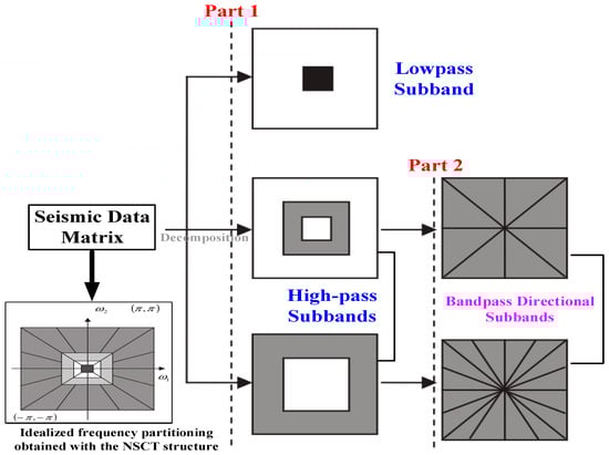
Figure 3.
NSCT diagram for 2D seismic data.
Figure 4 shows an example of the NSCT decomposition of noisy seismic data, resulting in multiple high-frequency sub-bands, each of which represents different high-frequency details in certain common directions. By summing these high-frequency sub-bands element-wise, a full-directional high-frequency sub-band is obtained, which can characterize both the global shape and local edge details of the seismic data simultaneously.
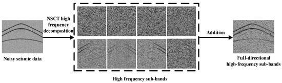
Figure 4.
Schematic diagram of NSCT high-frequency decomposition.
As shown in Figure 5, the seismic noise suppression problem is formulated as NSCT coefficient prediction to further remove noise by the FID-N while preserving more structural detail information compared with spatial-domain methods. This paper mentions that the NSCT can be an easy but effective tool for improving performance and can be used in various seismic noise-suppressing networks.
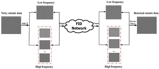
Figure 5.
Coefficient prediction in NSCT domain.
4. Experimental Results and Analysis
The present work qualitatively and quantitatively demonstrated the superior performance of our algorithm with experiments by comparing three popular contrasting algorithms, the wavelet transform [47], curvelet transform [3] and shearlet transform [49] seismic denoising algorithms, and six deep learning-based algorithms, the VDSR-based [16], MSRN-based [17], IDN-based [18], USRNET-based [22], TSAN-based [25], and D2UNet-based [41] data recovery algorithms, which were used for seismic data denoising in this paper.
4.1. Seismic Datasets and Experimental Details
To verify the performance of our algorithm, examples of hyperbolic events-synthesized signals were utilized, and the synthetic data generated with 150 traces and a 1 ms sampling interval are presented in Figure 6a. The Ricker wavelet is expressed by
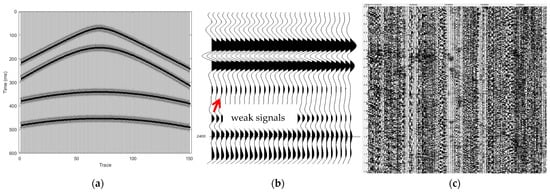
Figure 6.
(a) Original synthesized signals, (b) forward model, and (c) background noise.
The basic data for the experiments were synthesized seismic signals of 150 traces at a 1000 Hz sampling frequency with linear features, curvilinear features, different dip angles, and fault events. Figure 6a presents an example of the prepared records. In addition, we collected and obtained forward model data from 12 wells, including very weak effective signals, which aimed to verify the effectiveness of the proposed method for weak signal mining. Figure 6b presents an example of the forward models. This paper rotated the synthetic data and forward models by 45°, 90°, 135°, 180°, 270°, and 360°, and then added white Gaussian random noise and linear noise of various levels into the rotated synthetic data, as well as the original data, to generate additional expanded versions, which verified the effectiveness of the proposed method in removing random noise and linear noise simultaneously. Meanwhile, we added real background noise (Figure 6c) collected from unexcited seismic sources into the rotated forward models, as well as the original forward data, which verified the effectiveness of the proposed method for mining weak signals submerged in strong background noise. In total, 80% of the data were utilized as training sets, while the remaining data were adopted as testing sets. During the training process, the batch size was 64, and the initial learning rate was 10−4 for each layer and halved every 50 epochs. The experimental process was located in the HP 7920 series tower server, equipped with an NVIDIA RTX3090 graphics card, which can simultaneously process a large amount of noisy seismic data.
4.2. Comparison with State-of-the-Art (SOTA) Methods
In this subsection, the performance of the proposed algorithm on synthetic seismic data and forward models is evaluated, respectively. To improve comparability, all algorithms were trained using the same training set. The denoised data were justified quantitatively by using the evaluation metric of the peak signal-to-noise ratio (PSNR) [50]. Table 2 and Table 3 present the PSNR values (dB) for comparison with other state-of-the-art methods; values in bold font indicate optimal values. As shown in the tables, the PSNR values resulting from the deep learning-based methods were higher by a large margin quantitatively compared with the traditional methods, such as the wavelet, curvelet, and shearlet transform-based seismic denoising algorithms, especially with higher noise levels. Particularly, our method performed better in denoising with a higher PSNR value. Figure 7 and Figure 8 present the qualitative comparison results on the synthetic data and forward model data. Figure 7a shows the original synthetic data, and Figure 7b shows the data after adding white Gaussian random noise and linear noise. Figure 7c, Figure 7e and Figure 7g are the results processed by the shearlet algorithm, USRNET, and our method, respectively; Figure 7d,f,h are the corresponding eliminated noises. It is obvious that the resulting data of our method were closer to the original data, obtaining excellent qualitative results. Furthermore, Figure 8a shows a forward model of well data. We added real background noise to the forward model, as shown in Figure 8b. Figure 8c, Figure 8d and Figure 8e show the results processed by the IDN, the USRNET, and our method, respectively. We can see that our method achieved better results that were closer to the original forward model, and the weak signals were effectively restored compared with the other two methods.
Table 2.
Comparison of PSNR values on synthetic data for various algorithms.
Table 3.
Comparison of PSNR values for different methods on synthetic seismic data.
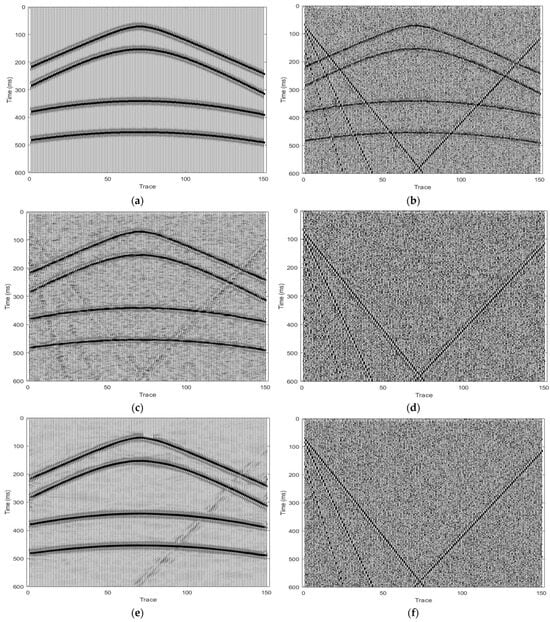
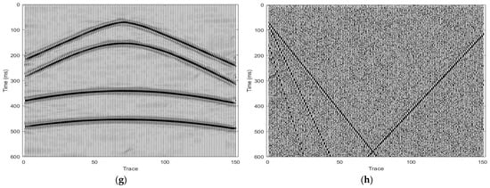
Figure 7.
Comparison of denoising results. Original (a) and noisy (b) synthetic data and denoised results processed by shearlet algorithm (c), USRNET (e), and our method (g), respectively. The corresponding eliminated noises are plotted in (d,f,h), respectively.
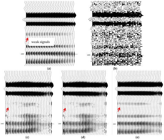
Figure 8.
Comparison of denoising results. Original forward model (a) and noisy forward model (b) and denoised results (c–e) processed by IDN, USRNET, and our method, respectively.
Next, we focus on evaluating the performance of our method on real seismic data. The FID-N worked well in low-SNR conditions, improving the signal quality by reducing noise and preserving important features. Figure 9 presents the processed comparison results of the original real seismic data with a low SNR. It can be seen that the effective signals processed by the commercial software were very limited due to noise. After denoising by our method, the effective signals became clearer. Figure 9b,c show the results processed by the commercial software and our method at high frequencies. For 40–80 Hz and 60–120 Hz, the results processed by the commercial software were not ideal, and our method could highlight the effective signals. On the contrary, the effective signals obtained by our method were obviously outstanding, improving the high-frequency SNR of the real seismic data. The FID-N preserved high-frequency details effectively, which are essential for detecting fine geological features. Furthermore, we processed the migrated profile data obtained by the seismic data processing flow, as shown in Figure 10. The red dashed line denotes the focusing target layer, under which the reservoir weak signal exists. However, the processing result of the commercial software was not obvious in terms of performance. We can clearly see that the result processed by our method presented more weak seismic signals and was better than that of the IDN, which provides significant contributions to the prediction of oil and gas reservoirs.
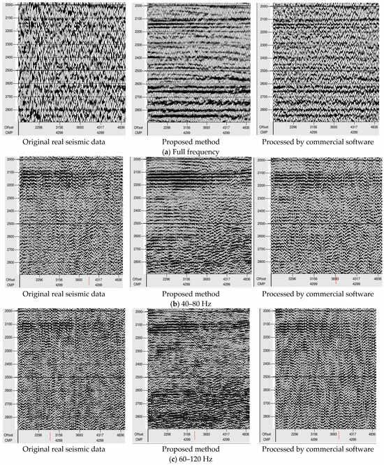
Figure 9.
Comparison of results processed by commercial software and our method for original real seismic data with a low SNR.
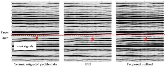
Figure 10.
Comparison of results processed by IDN and our method for seismic migrated profile data.
4.3. Ablation Studies
In this subsection, we first investigate the impact of iteration T in our FID-N network. As shown in Table 4, we found consistent performance improvements as the T value increased for synthetic data and forward model data. Considering the trade-off between accuracy and speed, we adopted T = 9 to construct the FID-N, which was used in the experiments. Second, we investigated the impact of our two-path information distillation block (IDB) and single-scale feature extraction. As shown in Table 5, we can see that our two-path IDB worked consistently better than single scaling. Furthermore, we evaluated the impact of the NSCT decomposition level on our FID-N’s performance. Since there were more high-frequency levels of decomposition and more directions, the overhead of the network increased accordingly. Therefore, we only discussed the decomposition of high-frequency levels within three. Considering the network overhead, we selected the results of NSCT decomposition at three levels. Table 6 shows the PSNR values corresponding to different high-frequency levels of NSCT decomposition. Obviously, with the increase in the decomposition level and the number of decomposition directions, the learned detailed information was richer, and the PSNR values increased accordingly.
Table 4.
Average PSNR values on synthetic data and forward models under different iterations T.
Table 5.
Comparison of average PSNR values on synthetic data and forward models for single-scale feature extraction and our two-path information distillation block (IDB).
Table 6.
Average PSNR values for different high-frequency levels of decomposition based on our FID-N.
5. Conclusions
We propose a novel CNN-based algorithm, FID-N, specifically designed to suppress seismic noise. Our method introduces several key innovations: (1) the use of a feedback structure combined with a two-path ID block, which significantly enhances the seismic denoising performance by effectively exploiting the inherent features of seismic signals; (2) the integration of an NSCT, which allows the network to retain fine-grained information from noisy seismic data, further improving denoising outcomes. The experimental results demonstrate that the FID-N consistently outperformed the SOTA methods, achieving higher PSNR values, particularly in scenarios with low SNR values. This highlights the superiority of our method, especially in preserving weak signals that are critical in seismic data analysis. Future work will focus on extending the FID-N to handle other types of noise and improving real-time processing capabilities.
Author Contributions
K.C., G.Z. and Q.R.: conceptualization, analysis, and framework construction. C.T. and L.W.: writing—review and editing, and investigation. S.H., H.L. and H.Y.: methodology, validation, and visualization. All authors have written, revised, and improved this paper. All authors have read and agreed to the published version of the manuscript.
Funding
This work was supported by the Major Science and Technology Project of PetroChina Company Limited (grant no. 2023ZZ16YJ04).
Institutional Review Board Statement
Not applicable.
Informed Consent Statement
Not applicable.
Data Availability Statement
The original contributions presented in the study are included in the article, further inquiries can be directed to the corresponding author.
Acknowledgments
We acknowledge all supporting organizations.
Conflicts of Interest
Authors Kang Chen, Cong Tang, Qi Ran, Long Wen, Song Han, Han Liang and Haiyong Yi were employed by PetroChina Southwest Oil & Gasfield Company. The remaining author declares that the research was conducted in the absence of any commercial or financial relationships that could be construed as a potential conflict of interest.
References
- Canales, L.L. Random noise reduction. In Proceedings of the 54th Annual International Meeting, Atlanta, GA, USA, 2 December 1984. [Google Scholar]
- Zhang, J.H.; Lu, J.M. Application of wavelet transform in removing noise and improving resolution of seismic data. J. Univ. Pet. Ed. Nat. Sci. 1997, 31, 1975–1981. [Google Scholar]
- Neelamani, R.; Baumstein, A.; Gillard, D.; Hadidi, M.; Soroka, W. Coherent and random noise attenuation using the curvelet transform. Lead. Edge 2008, 27, 240–248. [Google Scholar] [CrossRef]
- Chen, Y.; Ma, J. Random noise attenuation by f-x empirical mode decomposition predictive filtering. Geophysics 2014, 79, V81–V91. [Google Scholar] [CrossRef]
- Wang, B.; Wu, R.S.; Chen, X.; Li, J. Simultaneous seismic data interpolation and denoising with a new adaptive method based on treamlet transform. Geophys. J. Int. 2015, 201, 1182–1194. [Google Scholar] [CrossRef]
- Chen, Y.; Fomel, S. EMD-seislet transform. In Proceedings of the 85th SEG Annual International Meeting, New Orleans, LA, USA, 18–23 October 2015. [Google Scholar]
- Liu, W.; Cao, S.; Chen, Y.; Zu, S. An effective approach to attenuate random noise based on compressive sensing and curvelet transform. J. Geophys. Eng. 2016, 13, 135–145. [Google Scholar] [CrossRef]
- Liu, W.; Cao, S.; Chen, Y. Application of variational mode decomposition in random noise attenuation and time frequency analysis of seismic data. In Proceedings of the EAGE 78th Annual International Conference and Exhibition, Vienna, Austria, 30 May–2 June 2016. [Google Scholar]
- Beckouche, S.; Ma, J.W. Simultaneous dictionary learning and denoising for seismic data. Geophysics 2014, 79, A27–A31. [Google Scholar] [CrossRef]
- Zhou, Z.; Wu, J.; Bai, M.; Yang, B.; Ma, Z. Fast dictionary learning based on data-driven tight frame for 3-D seismic data denoising. IEEE Trans. Geosci. Remote Sens. 2024, 62, 5904510. [Google Scholar] [CrossRef]
- Bonar, D.; Sacchi, M. Denoising seismic data using the nonlocal means algorithm. Geophysics 2012, 77, A5–A8. [Google Scholar] [CrossRef]
- Yuan, Y.H.; Wang, Y.B.; Liu, Y.K.; Chang, X. Non-dyadic curvelet transform and its application in seismic noise elimination. Chin. J. Geophys. 2013, 56, 1023–1032. [Google Scholar]
- Zhou, Q.B.; Gao, J.H.; Wang, Z.G.; Li, K.X. Adaptive variable time fractional anisotropic diffusion filtering for seismic data noise attenuation. IEEE Trans. Geosci. Remote Sens. 2016, 54, 1905–1917. [Google Scholar] [CrossRef]
- Lin, C. Suppression of random noise in seismic data based on 3D Steerable Pyramid decomposition. Prog. Geophys. 2018, 33, 1081–1087. [Google Scholar]
- Genovese, F.; Palmeri, A. Wavelet-based generation of fully non-stationary random processes with application to seismic ground motions. Mech. Syst. Signal Process. 2025, 223, 111833. [Google Scholar] [CrossRef]
- Kim, J.; Lee, J.K.; Lee, K.M. Accurate image super-resolution using very deep convolutional networks. In Proceedings of the IEEE Conference on Computer Vision and Pattern Recognition (CVPR), Las Vegas, NV, USA, 26–30 June 2016. [Google Scholar]
- Li, J.C.; Fang, F.M.; Mei, K.F.; Zhang, G. Multi-scale residual network for image super-resolution. In Proceedings of the European Conference on Computer Vision (ECCV), Munich, Germany, 8–14 September 2018. [Google Scholar]
- Hui, Z.; Wang, X.M.; Gao, X.B. Fast and accurate single image super-resolution via information distillation network. In Proceedings of the IEEE Conference on Computer Vision and Pattern Recognition (CVPR), Salt Lake City, UT, USA, 18–23 June 2018. [Google Scholar]
- Wang, L.; Li, D.; Zhu, Y.S.; Tian, L.; Shan, Y. Dual Super-Resolution Learning for Semantic Segmentation. In Proceedings of the Computer Vision and Pattern Recognition, Seattle, WA, USA, 13–19 June 2020. [Google Scholar]
- Mustaqeem; Kwon, S. CLSTM: Deep feature-based speech emotion recognition using the hierarchical ConvLSTM network. Mathematics 2020, 8, 2133. [Google Scholar] [CrossRef]
- Sajjad, M.; Kwon, S. Clustering-based speech emotion recognition by incorporating learned features and deep BiLSTM. IEEE Access 2020, 8, 79861–79875. [Google Scholar]
- Zhang, K.; Gool, V.; Timofte, R. Deep unfolding network for image superresolution. In Proceedings of the IEEE/CVF Conference on Computer Vision and Pattern Recognition (CVPR), Seattle, WA, USA, 13–19 June 2020. [Google Scholar]
- Marco, P.; Marco, V.; Adrian, H. Attention-Based Multi-Reference Learning for Image Super-Resolution. In Proceedings of the International Conference on Computer Vision, Montreal, QC, Canada, 10–17 October 2021. [Google Scholar]
- Xie, W.B.; Song, D.H.; Xu, C.; Xu, C.J.; Zhang, H.; Wang, Y. Learning frequency-aware dynamic network for efficient super-resolution. In Proceedings of the International Conference on Computer Vision, Montreal, QC, Canada, 10–17 October 2021. [Google Scholar]
- Zhang, J.; Long, C.; Wang, Y.; Piao, H.; Mei, H.; Yang, X.; Yin, B. A two stage attentive network for single image super-resolution. IEEE Trans. Circuits Syst. Video Technol. 2022, 32, 1020–1033. [Google Scholar] [CrossRef]
- Liu, N.; Wang, J.; Gao, J.; Chang, S.; Lou, Y. NS2NS: Self-learning for seismic image denoising. IEEE Trans. Geosci. Remote Sens. 2022, 60, 1–13. [Google Scholar] [CrossRef]
- Zhang, C.; Frogner, C.; Araya-Polo, M. Machine-learning based automated fault detection in seismic traces. In Proceedings of the Conference of 76th EAGE Conference and Exhibition, Amsterdam, NL, USA, 19 June 2014. [Google Scholar]
- Cao, J.; Wu, S.; He, X. Gas reservoir identification basing on deep learning of seismic-print characteristics. In Proceedings of the AGU Fall Meeting, San Francisco, CA, USA, 12–16 December 2016. [Google Scholar]
- Huang, L.; Dong, X.; Clee, T.E. A scalable deep learning platform for identifying geologic features from seismic attributes. Lead. Edge 2017, 36, 249–256. [Google Scholar] [CrossRef]
- Olivier, G.; Chaput, J.; Borchers, B. Using supervised machine learning to improve active source signal retrieval. Seismol. Res. Lett. 2018, 89, 1023–1029. [Google Scholar] [CrossRef]
- Jia, Y.; Yu, S.; Ma, J. Intelligent interpolation by Monte Carlo machine learning. Geophysics 2018, 83, 83–97. [Google Scholar] [CrossRef]
- Zhang, P.L.; Li, Y.; Zhang, T.T. Study of seismic data denoising based on U-Net deep neural network. Met. Mine 2020, 1, 200–208. [Google Scholar]
- Mai, H. Research on Seismic Data Denoising Based on Deep Residual Network; China University of Petroleum: Beijing, China, 2019. [Google Scholar]
- Fang, W.Q.; Li, Z.M. Random noise attenuation in seismic data based on dual residual networks. Chin. J. Eng. Geophys. 2021, 18, 44–50. [Google Scholar]
- Yu, K. Research on Seismic Data Denoising Method Based on Symmetric Dilated Convolution Neural Network; Chengdu University of Technology: Chengdu, China, 2020. [Google Scholar]
- Sang, Y.; Sun, J.G.; Meng, X.F.; Peng, Y.F.; Jin, H.B. Seismic random noise attenuation based on PCC classification in transform domain. IEEE Access 2020, 8, 30368–30377. [Google Scholar] [CrossRef]
- Sang, Y.; Sun, J.G.; Gao, D.C.; Wu, H. Noise attenuation of seismic data via deep multiscale fusion network. Wirel. Commun. Mob. Comput. 2021, 2021, 6612346. [Google Scholar] [CrossRef]
- Sang, Y.; Yu, B.W.; Wang, Q.J.; Yin, S.S. Suppressing seismic coherent and incoherent noise via deep neural network. In Proceedings of the International Conference on Smart Internet of Things, Jeju, Republic of Korea, 1 August 2021. [Google Scholar]
- Li, J.; Wu, X.; Hu, Z. Deep learning for simultaneous seismic image super-resolution and denoising. IEEE Trans. Geosci. Remote Sens. 2022, 60, 5901611. [Google Scholar] [CrossRef]
- Chang, D.; Zhang, G.; Yong, X.; Gao, J.; Wang, Y.; Wang, W. Deep learning using synthetic seismic data by Fourier domain adaptation in seismic structure interpretation. IEEE Geosci. Remote Sens. Lett. 2022, 19, 8030705. [Google Scholar] [CrossRef]
- Min, F.; Wang, L.; Pan, S.; Song, G. D2UNet: Dual decoder U-Net for seismic image super-resolution reconstruction. IEEE Trans. Geosci. Remote Sens. 2023, 61, 5906913. [Google Scholar] [CrossRef]
- Li, F.; Liu, H.; Wang, W.; Ma, J. Swin transformer for seismic denoising. IEEE Geosci. Remote Sens. Lett. 2024, 21, 7501905. [Google Scholar] [CrossRef]
- Chen, J.; Chen, G.; Li, J.; Du, R.; Qi, Y.; Li, C.F.; Wang, N. Efficient seismic data denoising via deep learning with improved MCA-SCUNet. IEEE Trans. Geosci. Remote Sens. 2024, 62, 5903614. [Google Scholar] [CrossRef]
- Zhang, H.; Yang, J.; Huang, J.; Wang, W. An Adaptive Time-Frequency Denoising Method for Suppressing Source-Related Seismic Strong Noise. IEEE Trans. Geosci. Remote Sens. 2024, 62, 5908410. [Google Scholar] [CrossRef]
- Zamir, A.R.; Wu, T.L.; Sun, L.; Shen, W.B.; Shi, B.E.; Malik, J.; Savarese, S. Feedback networks. In Proceedings of the IEEE Conference on Computer Vision and Pattern Recognition (CVPR), Honolulu, HI, USA, 21 July 2017. [Google Scholar]
- Glorot, X.; Bordes, A.; Bengio, Y. Deep sparse rectifier neural networks. In Proceedings of the Artificial Intelligence and Statistics (AISTATS), Fort Lauderdale, FL USA, 11–13 April 2011. [Google Scholar]
- Mallat, S. A Wavelet Tour of Signal Processing: The Sparse Way; Academic Press: Cambridge, UK; New York, NY, USA, 2008. [Google Scholar]
- Labate, D.; Lim, W.Q.; Kutyniok, G.; Weiss, G. Sparse multidimensional representation using shearlets. In Proceedings of the Society of Photo-Optical Instrumentation Engineers (SPIE), Wavelets XI, Bellingham, WA, USA, 17 September 2005. [Google Scholar]
- DaCunha, A.L.; Zhou, J.; Do, M.N. The nonsubsampled contourlet transform: Theory, design, and applications. IEEE Trans. Image Process. 2006, 15, 3089–3101. [Google Scholar] [CrossRef]
- Wang, Z.; Bovik, A.C.; Sheikh, H.R.; Simoncelli, E. Image quality assessment: From error visibility to structural similarity. IEEE Trans. Image Process. 2004, 13, 600–612. [Google Scholar] [CrossRef] [PubMed]
Disclaimer/Publisher’s Note: The statements, opinions and data contained in all publications are solely those of the individual author(s) and contributor(s) and not of MDPI and/or the editor(s). MDPI and/or the editor(s) disclaim responsibility for any injury to people or property resulting from any ideas, methods, instructions or products referred to in the content. |
© 2025 by the authors. Licensee MDPI, Basel, Switzerland. This article is an open access article distributed under the terms and conditions of the Creative Commons Attribution (CC BY) license (https://creativecommons.org/licenses/by/4.0/).