Abstract
Underwater radiated noise power estimation is crucial for the quantitative assessment of noise levels emitted by ships and underwater vehicles. This paper therefore proposes a maximum likelihood estimation method for determining the power of underwater radiated noise. The method establishes the probability density function of the hydrophones array received data and derives the minimum variance unbiased estimation of the power through theoretical analysis under the maximum likelihood criterion. Numerical simulations and experimental data demonstrate that this method can significantly reduce the influence of ambient noise on estimation results and improve the estimation accuracy under low signal-to-noise ratio conditions, outperforming commonly used beamforming-based estimation methods. In addition, the estimation variance achieves the Cramér–Rao lower bound, which is consistent with theoretical derivation. When the source position is unknown, this method can simultaneously localize the sound source and estimate its power by searching for the maximum value within a specified region.
1. Introduction
With the rapid expansion of global shipping trade, ocean noise levels continue to rise annually [1,2,3,4,5]. Substantial research indicates that underwater radiated noise poses a significant threat to marine life, particularly marine mammals [6,7,8]. It can interfere with essential behaviors such as navigation, communication, and foraging. Prolonged exposure to elevated noise levels may also cause hearing damage and even cause fatalities in marine life. To mitigate these impacts of ocean noise pollution on marine ecosystems, the International Maritime Organization and various nations have implemented regulations limiting the radiated noise levels from marine vessels [9,10,11]. Consequently, measuring the radiated noise of ships and underwater vehicles prior to delivery is essential to assess whether their noise levels comply with design requirements and regulatory standards [12,13,14,15,16]. As a fundamental physical characteristic, the power of radiated noise provides the basis for calculating other quantities that describe the characteristics of underwater radiated noise, such as the source level, source band level, and source spectral level [17].
Due to cost and operational constraints, early measurements of underwater radiated noise predominantly employed single hydrophone systems, where the received sound pressure level was corrected via acoustic propagation loss to deduce the source level of the underwater radiated noise [18,19,20,21,22]. However, as underwater radiated noise levels decline while the ocean ambient noise level increases year by year, the Signal-to-Noise Ratio (SNR) of data received by a single hydrophone has progressively declined, leading to a gradual inability to meet measurement accuracy requirements [23,24,25,26]. To address this issue, methods based on hydrophone arrays have been developed that leverage the spatial directivity and array gain to reduce the influence of ambient noise on radiated noise measurements, thereby improving measurement accuracy [27,28,29]. Nevertheless, these methods typically assume plane-wave acoustic propagation, which differs from the actual shallow-water waveguide environment, leading to degraded performance on radiated noise power estimation in practical applications. Subsequently, a radiated noise measurement method based on conventional Matched-Field Processing (MFP) is proposed, which calculates the channel transfer function from the sound source to each element of the array via acoustic field models, exploiting multipath signals for improved accuracy [30]. However, this method remains susceptible to ambient noise effects under low SNR conditions. For such scenarios, a denoising method is used to estimate the signal covariance matrix prior to beamforming, effectively improving measurement accuracy [17,31,32].
Maximum Likelihood Estimation (MLE) is one of the most fundamental and widely used parameter estimation methods in statistics [33,34]. Its core principle is to find the parameter value that maximizes the probability of the observed data. This paper applies it to the measurement of underwater radiated noise and proposes a maximum likelihood estimation method for underwater radiated noise power. Unlike conventional methods for radiated noise measurement based on array signal processing, the proposed method firstly establishes the probability density function of the received data under the assumption of white Gaussian noise. Subsequently, an estimation of the radiated noise power, which conforms to the maximum likelihood criterion, is derived and validated as the minimum variance unbiased estimation. Compared to conventional radiated noise measurement methods, the proposed MLE is the optimal estimation, providing the optimal estimation accuracy for the underwater radiated noise power.
The rest of the paper is organized as follows. Section 2 introduces the receiving data model with a Vertical Linear Array (VLA). Section 3 reviews several common radiated noise power estimation methods based on beamforming. Section 4 establishes the probability density function of the array-received data and develops the MLE method, and Section 5 derives the Cramér–Rao Lower Bound (CRLB). In Section 6, the effects of different parameters on MLE performance are investigated through numerical simulations, with performance comparisons against the methods introduced in Section 3. Section 7 further validates the practical efficacy of MLE using experimental data. Finally, Section 8 provides a summary.
2. Data Model
Assuming that the underwater radiated noise source can be approximated as a point source, and considering the effects of shallow-water sound propagation, the time-domain data received by a single hydrophone can be expressed as the convolution of the channel impulse response and the radiated noise [35]:
where denotes convolution, represents the radiated noise at a distance of 1 m from the source, denotes the channel impulse response from the source to the hydrophone at the position , and represents the ambient noise received by the hydrophone. In this study, it is assumed that both the radiated noise and the ambient noise are characterized as white Gaussian noise and are mutually independent.
By segmenting the received time-domain data and applying the Discrete Fourier Transform (DFT), the frequency-domain received data is obtained and expressed as
where denotes the time-segment index, denotes the signal frequency, , and represent the DFTs of the hydrophone data , the underwater radiated noise , and the ambient noise , respectively, and is the channel transfer function from the radiated noise source to the hydrophone at frequency .
In practice, an array composed of multiple hydrophones is employed for data acquisition, thereby achieving beamforming gain to enhance the SNR of the received data. For an M-element hydrophone array, the received data can be expressed as
where the subscript . indicates the index of each hydrophone.
Due to the influence of the ocean channel, the signal power received by various array hydrophones may vary. Consequently, the SNR of the array received data is defined by utilizing the average power of the received signal and the ambient noise across the entire array as
where denotes the square of the norm of a vector, represents the power of the radiated noise, and represents the average power of the ambient noise received by the M-element array.
3. Beamforming-Based Power Estimation Methods
For comparison, the commonly used beamforming-based power estimation methods for underwater radiated noise are first reviewed. First, the beamforming is performed to the array received data, and the output signal is expressed as [35]
where is a simplified notation of , denotes the weighting vector, and the superscript represents the conjugate transpose. Then the beamforming output power is expressed as
In Equation (6), denotes the covariance matrix of the received data, where is the expectation operator, is the covariance matrix of the received radiated noise, and is the covariance matrix of the ambient noise. The approximation means that the power of ambient noise is negligible, which is reasonable when the SNR of the beamforming output is high. So the power of the radiated noise is given by
3.1. Conventional Beamforming
Under the far-field assumption, the estimated channel transfer function and the weighting vector can be expressed as
where denotes the reference hydrophone index, is the distance between the reference hydrophone and the sound source, is the wavenumber, is the inter-element spacing, and is the bearing angle of the source relative to the array. Substituting Equation (8) to Equation (7) yields the Conventional BeamForming (CBF) estimate of radiated noise power
3.2. Near-Field Focused Beamforming
In the near-field, the estimated channel transfer function and the weighting vector can be expressed as
where is the distance between the m-th hydrophone and the source. Substituting Equation (10) to Equation (7), the radiated noise power estimate with Near-field Focused BeamForming (NFBF) is given by
3.3. Matched-Field Processing
For matched-field processing, the weighting vector is typically represented as the normalized form of the channel transfer function:
where denotes the norm of a vector. Substituting the weighting vector to Equation (7), the power estimate with MFP is expressed as [30]
3.4. RPCA-Based Denoising Approach
Since the derivation of Equation (6) neglects the influence of ambient noise, the measurement error becomes significant when the beamforming output SNR is low. Consequently, denoising methods can be applied first to suppress the ambient noise before estimating the radiated noise power. The Robust Principal Component Analysis (RPCA) method can be used to estimate the signal covariance matrix and the noise covariance matrix simultaneously. The optimization formulation can be expressed as [31]
where and denote the nuclear norm and the norm, respectively, denotes the regularization parameter, and means the matrix is a positive semi-definite matrix. Then substituting the estimated signal covariance matrix into Equation (11), the radiated noise power estimate is expressed as
4. Maximum Likelihood Estimation Method
Differing from beamforming-based approaches, this section introduces a radiated noise power estimation method based on probability density maximization. Since the array elements are mutually independent, the signal received by the array follows a joint normal distribution. In the complex domain, the Probability Density Function (PDF) is expressed as [36]
where denotes the determinant of a matrix.
For the received independent and identically distributed frequency snapshots, the corresponding joint PDF is
For the matrix , it can be transformed into
where is the identity matrix. For the rank-1 matrix in Equation (18), it has only one non-zero eigenvalue . Additionally, since the sum of all eigenvalues of a matrix equals its trace, it follows that
where denotes the trace of a matrix. Moreover, as the determinant of a matrix is equal to the product of all its eigenvalues, then
According to the matrix inversion lemma, the inverse of the matrix can be expressed as
Substituting Equations (20) and (21) into Equation (17), and additionally, to facilitate computations, Equation (17) is represented in logarithmic form as
In Equation (22),
where denotes the sampling covariance matrix of the received data.
To find the parameter that maximizes Equation (22), by substituting Equation (23) into Equation (22) and taking the partial derivative of the resulting expression with respect to the parameter [36], one obtains
By setting Equation (24) as equal to 0, the estimation of can be obtained, expressed as
For Equation (25), it can be interpreted as the outputs of Minimum Variance Distortionless Response (MVDR) beamforming of the covariance matrix difference between the received data and the ambient noise, thereby eliminating the influence of ambient noise on the estimation. Additionally, the ambient noise covariance matrix for radiated noise power estimation can be obtained by collecting ambient noise before radiated noise measurement. The channel transfer function can be calculated from marine environmental parameters using acoustic field simulation toolbox, such as the KrakenC program based on normal mode [37,38] in the Acoustics Toolbox [39]. The toolbox we are using was updated on 4 November 2020. Combining these with the sampling covariance matrix of the received data , the radiated noise power can be accurately determined.
5. The Cramér–Rao Lower Bound Derivation
To analyze the estimation performance of the proposed method, we theoretically verified whether its estimation variance achieves the CRLB. First, the theoretical value of CRLB is derived. For Equation (24), taking the second partial derivative with respect to the parameter yields
According to Reference [36], the Fisher information matrix can be obtained by taking the negative expectation of Equation (26), denoted as
where . Subsequently, the CRLB can be calculated and represented as
Subsequently, we prove that the proposed power estimation method achieves the CRLB. For Equation (24), it can be transformed into
According to CRLB theorem [36], the variance of estimation meets the CRLB. In addition, the expectation of Equation (25) is given by
Thus, it can be inferred that is the Minimum Variance Unbiased Estimation (MVUE) of .
6. Numerical Simulation Results Analysis
The simulated shallow-water waveguide environment is depicted in Figure 1. The 100 m water column overlies a 10 m sediment layer, with the sound speed profile annotated in the figure. Key environmental parameters affecting acoustic propagation, including sound speed, density, and attenuation coefficients, are specified in the diagram. The radiated noise is assumed to be a single-frequency signal at 750 Hz with the power of 90 dB. The sound source marked by a black pentagram in the figure is located at a depth of 50 m. The receiving hydrophone array marked by a set of black solid circles is a 31-element VLA with half-wavelength inter-element spacing. The central depth of the array is 50 m, and it is horizontally situated 100 m away from the radiated noise source. The ambient noise is set as white Gaussian noise with a power of 60 dB.
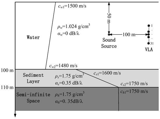
Figure 1.
The sketch of a typical shallow-water waveguide environment that is used in the following simulations.
In the following simulations, we compare the proposed MLE method against conventional beamforming approaches: CBF, NFBF, MFP, and an RPCA-based denoising method. Performance is systematically evaluated across varying conditions using the estimated variance, calculated as
where represents the average of N estimated values, and N is the number of Monte Carlo trials. In the following simulations, the number of Monte Carlo trials N is taken as 10,000. For the convenience of numerical display, the logarithm of the calculated variance is represented in the picture.
6.1. Impact of SNR on Estimation Results
The SNR of the received data is a critical factor influencing the radiated noise estimation results. It can be altered by adjusting the power of the radiated noise. The power of the radiated noise varies within the range of 70 to 110 dB, and the corresponding SNR of the received data is shown in Figure 2. Furthermore, the estimation results and estimation variances through different methods are shown in Figure 3.
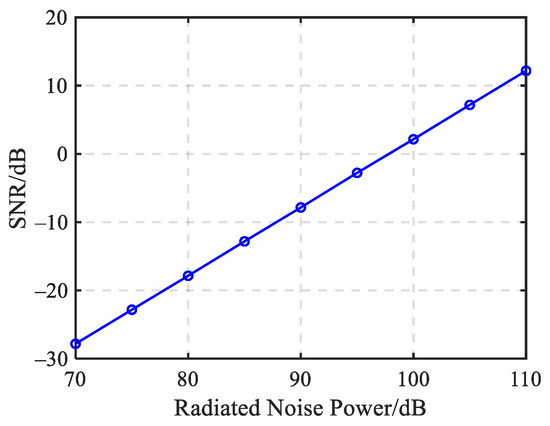
Figure 2.
The SNR of the received data corresponding to different radiated noise power.
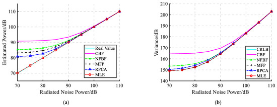
Figure 3.
Radiated noise estimation results under different radiated noise power, (a) estimation results, (b) estimation variances.
It can be seen that the SNR of the received data varies linearly with the radiated noise power. The estimation errors of different methods decrease as the radiated noise power increases, and the estimation variances tend towards CRLB with the increasing power. Among these methods, the CBF method exhibits the highest estimation error and variance, primarily due to the failure of the far-field assumption at close ranges. Consequently, the NFBF method effectively reduces the estimation error caused by range mismatch compared to CBF, but its measurement error remains relatively large. The MFP method achieves the CRLB in terms of estimation variance under different radiated noise power, while its estimation error is relatively larger at lower radiated noise level due to the influence of ambient noise. The RPCA method reduces the impact of ambient noise through denoising, thereby decreasing the estimation error, but its estimation variance remains higher than CRLB. In contrast, the MLE method is least affected by variations in the radiated noise power, providing the most accurate estimation results. Moreover, its estimation variance reaches the CRLB, demonstrating the optimal estimation performance.
6.2. Impact of Snapshot Number on Estimation Results
The proposed radiated noise power estimation method necessitates the use of the ambient noise covariance matrix, which can be estimated through prolonged monitoring of ambient noise. However, when the number of snapshots in Equation (17) is limited, discrepancies may arise between the actual noise covariance matrix and the sampling covariance matrix, potentially affecting the estimation accuracy. Figure 4 presents the estimation results and variances of radiated noise for different snapshot numbers.
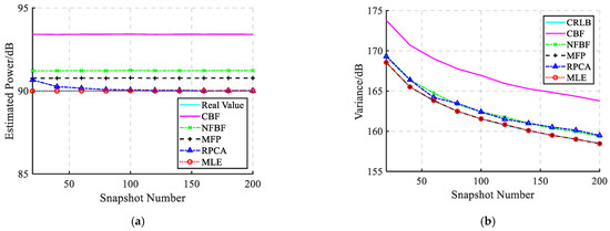
Figure 4.
Radiated noise estimation results under different snapshot numbers, (a) estimation results, (b) estimation variances.
It can be observed that, except for the RPCA method, the estimation results of the other methods remain constant regardless of the number of snapshots, while their estimation variances decrease as the number of snapshots increases. Among these methods, the CBF and NFBF methods exhibit the largest estimation errors and variances. The estimation variance of the MFP method achieves CRLB, but its estimation error remains relatively large. The denoising performance of the RPCA method improves with the increasing number of snapshots [32], thereby enhancing the estimation accuracy, although its estimation variance remains relatively large. In contrast, the MLE method achieves optimal performance in both estimation result and variance, reaching the CRLB and demonstrating the best estimation performance.
6.3. Impact of Signal Frequency on Estimation Results
For an array with fixed inter-element spacing, the beam patterns of different beamforming methods vary with frequency, raising the question of whether this variability affects the performance of beamforming-based methods for estimating radiated noise power. Additionally, it is also worth discussing whether the MLE method is subject to this issue. Due to variations in the channel transfer functions at different frequencies, the SNR of the received data fluctuates. For a VLA with 1 m inter-element spacing, Figure 5 presents the SNR of the received data under different frequency conditions, and Figure 6 provides the estimation results and variances.
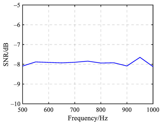
Figure 5.
The SNR of received data at different frequencies.
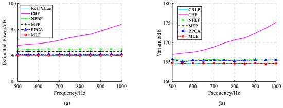
Figure 6.
Radiated noise estimation results at different frequencies, (a) estimation results, (b) estimation variances.
It can be observed that the SNR of the received data remains nearly constant at different frequencies. Except for the CBF method, the estimation results and variances of the other methods are largely unaffected by frequency variations. For the CBF method, based on the Fraunhofer distance condition under the far-field assumption, it becomes increasingly challenging to satisfy the far-field condition as the frequency rises at a fixed distance. This leads to a rise in both estimation error and variance at higher frequencies. The NFBF method exhibits relatively large estimation error and variance, while the MFP method achieves the CRLB but still suffers from significant estimation error. The RPCA method demonstrates relatively smaller estimation error and variance. In contrast, the MLE method achieves the smallest estimation error, and its estimation variance reaches CRLB, thereby demonstrating optimal performance in radiated noise estimation.
6.4. Impact of the Unknown Sound Position on Estimation Results
In previous simulations, it was assumed that the source position was known. However, in practical scenarios, deviation in the target position can occur. Under such conditions, it is necessary to evaluate the performance of radiated noise estimation at different assumed positions. Figure 7 presents the estimation results of the radiated noise power using channel transfer functions at different positions.
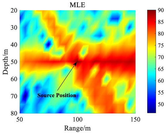
Figure 7.
Radiated noise estimation results at different assumed positions.
It can be observed that the position with the highest estimated power corresponds to the actual position of the sound source, and the estimation result matches the true power of the radiated noise. It indicates that the proposed MLE method remains applicable even when the source position is unknown.
7. Experiment Validation
In this section, the performance of MLE on underwater radiated noise measurement is validated using experimental data. The experiment was implemented in a reservoir in December 2019 [32]. Figure 8 illustrates the reservoir environment, as well as the geometric configuration of the source and receiving array. The sound speed profile was measured using a CTD sensor. The properties of the sediment layer and semi-infinite layer, including sound speed, density, and attenuation coefficients, were determined based on seabed material. A UW-350 transducer submerged at a depth of 50 m emitted two types of signals: (1) a 750 Hz Continuous Wave (CW) tone, and (2) a 10 s duration Linear Frequency Modulated (LFM) pulse with a frequency range of 100–900 Hz. A nested vertical hydrophone array, comprising a 24-element uniform linear subarray with a 1 m spacing and a 17-element subarray with a 0.5 m spacing, was deployed vertically at a horizontal range of 34.5 m from the source, spanning depths from 73 to 97 m. Additionally, a reference hydrophone, located at the same 50 m depth as the source but horizontally offset by 5.2 m, was used to monitor the source level. Due to the short propagation distance, the recorded signals exhibited high SNRs, allowing the single hydrophone-derived power estimates to serve as real value for radiated signal validation. All data were sampled at 48 kHz.
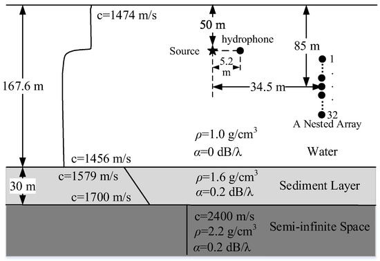
Figure 8.
The sketch of the experimental reservoir environment and the configuration of the source (marked by a black pentagram) and the array (marked by a set of black solid circles).
During post-processing, data from the central 15 hydrophones of the nested array with 1 m inter-element spacing were analyzed. To investigate the impact of snapshot number on measurement performance, the CW signal duration was varied from 2 s to 10 s. Frequency-domain conversion was performed via DFT with a 0.2 s rectangular window and 50% overlap. Figure 9a presents the estimated powers of CW signal across different snapshot numbers, while Figure 9b shows the corresponding estimation biases. These experimental results are basically consistent with the simulated trends in Figure 4a. It can be seen that the estimation bias of RPCA exhibits a decreasing trend as snapshot numbers increase. Moreover, the MLE method demonstrates the best estimation performance, highlighting its superior robustness to snapshot limitations compared to other methods.
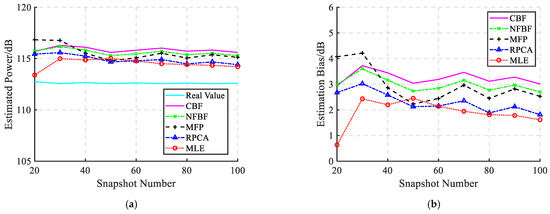
Figure 9.
(a) The estimated powers and (b) estimation biases of the CW signal with different snapshot numbers.
To comparatively evaluate frequency-dependent performance, the power and associated estimation biases of the LFM signal across the 500–900 Hz are analyzed. The results are presented in Figure 10. The comparative analysis reveals that MLE achieves the closest agreement with real values across the entire frequency band. However, it should be noted that under specific spectral regions, MLE exhibits a slight negative bias, likely caused by noise covariance matrix mismatch. In contrast, other methods demonstrate bias fluctuations exceeding 3 dB.
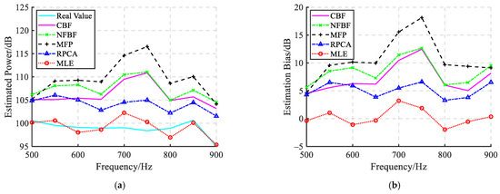
Figure 10.
(a) The estimated powers and (b) estimation biases of the LFM signal at different frequencies.
8. Conclusions
Underwater radiated noise measurement plays a crucial role in assessing the radiated noise levels of marine vessels. Unlike measurement methods based on array beamforming, this paper approaches the problem from a probabilistic perspective, proposing a MLE method for underwater radiated noise power. Assuming white Gaussian noise, the PDF representation of the hydrophone array received data is established, and the radiated noise power estimation under the maximum likelihood criterion is derived.
Theoretical derivation proves that this estimate is a MVUE, satisfying the CRLB. Numerical simulation results indicate that the proposed method exhibits reduced susceptibility to ambient noise and maintains optimal power estimation performance even under low SNR conditions. Experimental data further verifies the effectiveness of this estimation method in practical measurement applications.
Additionally, when the source location is unknown, the method can still locate the source and estimate its power by searching for the peak value within a specified area. However, due to the necessity of employing the ambient noise covariance matrix, the method is more suitable for fixed measurement sites with stationary ambient noise, as the statistical covariance matrix of ambient noise can be obtained through prolonged monitoring.
For future work, (1) it is necessary to consider that ship-radiated noise sources are not a point source in realistic scenarios, but rather volume sources composed of multipoint sources; and (2) considering the fluctuations in ocean environmental parameters, the robustness of this method to changes in environmental parameters needs to be analyzed.
Author Contributions
Conceptualization, G.J. and M.L.; methodology, G.J. and M.L.; software, G.J., Z.L. and L.S.; validation, G.J. and Z.L.; formal analysis, G.J. and L.S.; investigation, G.J.; resources, G.J.; data curation, G.J. and Z.L.; writing—original draft preparation, G.J.; writing—review and editing, G.J. and M.L.; visualization, G.J.; supervision, Q.W.; project administration, Q.W. All authors have read and agreed to the published version of the manuscript.
Funding
This research received no external funding.
Institutional Review Board Statement
Not applicable.
Informed Consent Statement
Not applicable.
Data Availability Statement
The data presented in this study are available on request from the corresponding author.
Acknowledgments
The authors are grateful to the anonymous reviewers.
Conflicts of Interest
The authors declare no conflicts of interest.
Abbreviations
The following abbreviations are used in this manuscript:
| MLE | Maximum Likelihood Estimation |
| MVUE | Minimum Variance Unbiased Estimation |
| CRLB | Cramér–Rao Lower Bound |
| SNR | Signal-to-Noise Ratio |
| Probability Density Function | |
| MFP | Matched-Field Processing |
| CBF | Conventional BeamForming |
| NFBF | Near-field Focused BeamForming |
| VLA | Vertical Linear Array |
| RPCA | Robust Principal Component Analysis |
References
- McDonald, M.A.; Hildebrand, J.A.; Wiggins, S.M. Increases in deep ocean ambient noise in the Northeast Pacific west of San Nicolas Island, California. J. Acoust. Soc. Am. 2006, 120, 711–718. [Google Scholar] [CrossRef]
- Frisk, G.V. Noiseonomics: The relationship between ambient noise levels in the sea and global economic trends. Sci. Rep. 2012, 2, 437. [Google Scholar] [CrossRef]
- ZoBell, V.M.; Hildebrand, J.A.; Frasier, K.E. Comparing pre-industrial and modern ocean noise levels in the Santa Barbara Channel. Mar. Pollut. Bull. 2024, 202, 116379. [Google Scholar] [CrossRef]
- Basan, F.; Fischer, J.G.; Putland, R.; Brinkkemper, J.; de Jong, C.A.F.; Binnerts, B.; Narro, A.; Kühnel, D.; Ødegaard, L.-A.; Andersson, M.; et al. The underwater soundscape of the North Sea. Mar. Pollut. Bull. 2024, 198, 115891. [Google Scholar] [CrossRef]
- Guo, C.; Wang, X.; Chen, C.; Li, Y.; Hu, J. Numerical investigation of self-propulsion performance and noise level of DARPA Suboff model. J. Mar. Sci. Eng. 2023, 11, 1206. [Google Scholar] [CrossRef]
- Ramesh, K.; Berrow, S.; Meade, R.; O’ Brien, J. Habitat modelling on the potential impacts of shipping noise on fin whales (Balaenoptera physalus) in offshore Irish waters off the Porcupine Ridge. J. Mar. Sci. Eng. 2021, 9, 1207. [Google Scholar] [CrossRef]
- Beck, S.; O’ Brien, J.; Berrow, S.; O’ Connor, I.; Wall, D. The Effects of Noise on Aquatic Life II; Springer: New York, NY, USA, 2016. [Google Scholar]
- Li, S.; Wu, H.; Xu, Y.; Peng, C.; Fang, L.; Lin, M.; Xin, L.; Zhang, P. Mid-to high-frequency noise from high-speed boats and its potential impacts on humpback dolphins. J. Acoust. Soc. Am. 2015, 138, 942–952. [Google Scholar] [CrossRef]
- Meier-Wehren, B. The global programme of action for the protection of the marine environment from land-based activities. N. Z. J. Environ. Law 2013, 17, 1. [Google Scholar]
- McCarthy, E. International Regulation of Underwater Sound: Establishing Rules and Standards to Address Ocean Noise Pollution; Springer Science & Business Media: Berlin, Germany, 2007. [Google Scholar]
- Badino, A.; Borelli, D.; Gaggero, T.; Rizzuto, E.; Schenone, C. Normative framework for ship noise: Present and situation and future trends. Noise Control Eng. J. 2012, 60, 740–762. [Google Scholar] [CrossRef]
- Cao, H.; Wen, L. High-precision numerical research on flow and structure noise of underwater vehicle. Appl. Sci. 2022, 12, 12723. [Google Scholar] [CrossRef]
- ABS. Guide for the Classification Notation Underwater Noise; American Bureau of Shipping: Houston, TX, USA, 2018. [Google Scholar]
- DNV-GL. Measurement Procedures for Noise Emission; Det Norske Veritas: Høvik, Norway, 2019. [Google Scholar]
- BV. Underwater Radiated Noise (URN); Bureau Veritas: Paris, France, 2018. [Google Scholar]
- LR. Additional Design and Construction Procedure for the Determination of a Vessel’s Underwater Radiated Noise; Lloyd’s Register: London, UK, 2018. [Google Scholar]
- Jiang, G.Q.; Sun, C.; Liu, X.; Jiang, G.Y. Radiated noise measurement by a small-aperture vertical array based on robust principal component analysis. J. Harbin Eng. Univ. 2020, 41, 1493–1499. [Google Scholar] [CrossRef]
- ISO 17208-1:2016; Underwater Acoustics—Quantities and Procedures for Description and Measurement of Underwater Sound from Ships—Part 1: Requirements for Precision Measurements in Deep Water Used for Comparison Purposes. ISO: Geneva, Switzerland, 2016.
- ISO 17208-2:2019; Underwater Acoustics—Quantities and Procedures for Description and Measurement of Underwater Sound from Ships—Part 2: Determination of Source Levels from Deep Water Measurements. ISO: Geneva, Switzerland, 2019.
- MacGillivray, A.O.; Martin, S.B.; Ainslie, M.A.; Dolman, J.N.; Li, Z.; Warner, G.A. Measuring vessel underwater radiated noise in shallow water. J. Acoust. Soc. Am. 2023, 153, 1506–1524. [Google Scholar] [CrossRef] [PubMed]
- Brooker, A.; Humphrey, V. Measurement of radiated underwater noise from a small research vessel in shallow water. Ocean Eng. 2016, 120, 182–189. [Google Scholar] [CrossRef]
- Jansen, E.; de Jong, C. Experimental assessment of underwater acoustic source levels of different ship types. IEEE J. Ocean. Eng. 2017, 42, 439–448. [Google Scholar] [CrossRef]
- Zhang, G.; Forland, T.N.; Johnsen, E.; Pedersen, G.; Dong, H. Measurements of underwater noise radiated by commercial ships at a cabled ocean observatory. Mar. Pollut. Bull. 2020, 153, 110948. [Google Scholar] [CrossRef]
- Cope, S.; Hines, E.; Bland, R.; Davis, J.D.; Tougher, B.; Zetterlind, V. Multi-sensor integration for an assessment of underwater radiated noise from common vessels in San Francisco Bay. J. Acoust. Soc. Am. 2021, 149, 2451–2464. [Google Scholar] [CrossRef]
- Zhu, S.; Zhang, G.; Wu, D.; Jia, L.; Zhang, Y.; Geng, Y.; Liu, Y.; Ren, W.; Zhang, W. High signal-to-noise ratio MEMS noise listener for ship noise detection. Remote Sens. 2023, 15, 777. [Google Scholar] [CrossRef]
- Helal, K.M.; von Oppeln-Bronikowski, N.; Moro, L. Advancing glider-based acoustic measurements of underwater-radiated ship noise. J. Acoust. Soc. Am. 2024, 156, 2467–2484. [Google Scholar] [CrossRef]
- Fillinger, L.; Sutin, A.; Sedunov, A. Acoustic ship signature measurements by cross-correlation method. J. Acoust. Soc. Am. 2011, 129, 774–778. [Google Scholar] [CrossRef]
- Wang, L.S.; Robinson, S.P.; Theobald, P.; Lepper, P.A.; Hayman, G.; Humphrey, V.F. Measurement of radiated ship noise. In Proceedings of the Meetings on Acoustics, Edinburgh, UK, 2–6 July 2012. [Google Scholar] [CrossRef]
- Jeong, H.; Lee, J.-H.; Kim, Y.-H.; Seol, H. Estimation of the noise source level of a commercial ship using on-board pressure sensors. Appl. Sci. 2021, 11, 1243. [Google Scholar] [CrossRef]
- Xiang, L.; Sun, C. An estimation method of ship radiated noise level based on matched field processing. Chin. J. Acoust. 2014, 39, 570–576. [Google Scholar] [CrossRef]
- Amailland, S.; Thomas, J.H.; Pézerat, C.; Boucheron, R. Boundary layer noise subtraction in hydrodynamic tunnel using robust principal component analysis. J. Acoust. Soc. Am. 2018, 143, 2152–2163. [Google Scholar] [CrossRef] [PubMed]
- Jiang, G.; Sun, C.; Xie, L. Diagonal denoising for spatially correlated noise based on diagonalization decorrelation in underwater radiated noise measurement. J. Mar. Sci. Eng. 2022, 10, 502. [Google Scholar] [CrossRef]
- Myung, I.J. Tutorial on maximum likelihood estimation. J. Math. Psychol. 2003, 47, 90–100. [Google Scholar] [CrossRef]
- Liu, Y.; Liu, B. A modified uncertain maximum likelihood estimation with applications in uncertain statistics. Commun. Stat.—Theory Methods 2024, 53, 6649–6670. [Google Scholar] [CrossRef]
- Van Trees, H.L. Optimum Array Processing: Part IV of Detection, Estimation, and Modulation Theory; John Wiley & Sons: New York, NY, USA, 2002. [Google Scholar]
- Kay, S.M. Fundamentals of Statistical Signal Processing, Volume I: Estimation Theory; Prentice Hall PTR: Hoboken, NJ, USA, 1993. [Google Scholar]
- Porter, M.B.; Reiss, E.L. A numerical method for bottom interacting ocean acoustic normal modes. J. Acoust. Soc. Am. 1985, 77, 1760–1767. [Google Scholar] [CrossRef]
- Porter, M.B. The KRAKEN Normal Mode Program; Naval Research Lab: Washington, DC, USA, 1992. [Google Scholar]
- Porter, M.B. Acoustics Toolbox. Available online: http://oalib.hlsresearch.com/AcousticsToolbox/index.html (accessed on 11 June 2025).
Disclaimer/Publisher’s Note: The statements, opinions and data contained in all publications are solely those of the individual author(s) and contributor(s) and not of MDPI and/or the editor(s). MDPI and/or the editor(s) disclaim responsibility for any injury to people or property resulting from any ideas, methods, instructions or products referred to in the content. |
© 2025 by the authors. Licensee MDPI, Basel, Switzerland. This article is an open access article distributed under the terms and conditions of the Creative Commons Attribution (CC BY) license (https://creativecommons.org/licenses/by/4.0/).