Hybrid Hydrological Forecasting Through a Physical Model and a Weather-Informed Transformer Model: A Case Study in Greek Watershed

Abstract

This study explores a hybrid AI framework for streamflow forecasting that integrates physically based hydrological modeling, bias correction, and deep learning. HEC-HMS simulations generate synthetic discharge, which a machine learning-based bias correction model adjusts for irrigation-induced discrepancies—improving the Nash–Sutcliffe Efficiency (NSE) from 0.55 to 0.84, the Kling–Gupta Efficiency (KGE) from 0.67 to 0.89, and reducing the RMSE from 1.084 to 0.301 m³/s. The corrected discharge is used as input to a Temporal Fusion Transformer (TFT) trained on hourly meteorological data to predict streamflow at 24-, 48-, and 72-h horizons. In a semi-arid, irrigated basin in Northern Greece, the TFT achieves NSEs of 0.84, 0.78, and 0.71 and RMSEs of 0.301, 0.743, and 0.980 m³/s, respectively. Probabilistic forecasts deliver uncertainty bounds with coverage near nominal levels. In addition, the model’s built-in interpretability reveals temporal and meteorological influences—such as precipitation—that enhance predictive performance. This framework demonstrates the synergistic benefits of combining physically based modeling with state-of-the-art deep learning to support robust, multi-horizon forecasts in irrigation-influenced, data-scarce environments.

1. Introduction

Water stands as one of the most crucial natural resources globally, with the provision of safe and clean drinking water recognized as a fundamental human right [1,2]. However, growing challenges are anticipated, particularly concerning droughts and water quality, which are driven by the combined forces of climate change, rising water demand due to population growth, and rapid urbanization [3,4]. Unsustainable water resource development in large river basins has led to significant environmental issues and geohazards such as soil salinization, land degradation, earth fissures, and ground subsidence [5,6]. As a result, the sustainable development and management of water resources in major basins has become a critical global priority, requiring in-depth and coordinated scientific research.

Furthermore, climate change is directly influencing weather patterns, with wide-ranging environmental, economic, and social consequences—such as biodiversity loss and increased insurance costs in flood-prone areas. The increasing frequency and severity of devastating floods has become an urgent concern. In September 2023, Storm Daniel, a powerful and unprecedented weather system, brought record-breaking rainfall to countries across the Mediterranean region, including Greece, Turkey, Libya, and Bulgaria. It was the deadliest Mediterranean tropical-like cyclone ever recorded, resulting in significant loss of life and widespread infrastructure damage. Additionally, Storm Daniel became the most expensive tropical cyclone ever recorded outside the North Atlantic. These events highlight the impacts that extreme flooding can impose on societies, economies, and ecosystems.

It is therefore clear that the need for effective hydrological models is more evident than ever. The severe impacts of recent extreme weather events, including both devastating floods and prolonged droughts, emphasize the pressing need for innovation in this domain. While traditional hydrological forecasting systems remain important, they often fall short in delivering timely and precise predictions. These systems face difficulties in responding to emerging hazards, supporting efficient disaster management, and adapting to the growing complexity of environmental conditions driven by climate change.

In parallel, a particular challenge in hydrological prediction is the limitation of available streamflow measurements. The available data in a plethora of basins are insufficient, inconsistent, or biased due to human activity. This “ungauged basin problem” is especially critical in regions prone to flash floods or in developing areas where monitoring infrastructure is limited [7]. Researchers have traditionally addressed this issue using physical models, which can simulate watershed processes based on fundamental hydrological principles. This work addresses the middle ground where a framework partially dependent on real data can be utilized to fill in the gaps and deliver operational streamflow forecasts.

The integration of physical modeling approaches with deep learning techniques presents a promising path forward for hydrological prediction. The simulated streamflow data from these physical models could potentially serve as additional training data for deep learning approaches. Since neural networks’ performance typically scales with the amount of training data available, the synthetic data generated by physical models could enhance the deep learning model’s predictive capabilities by providing additional training examples that are physically consistent with watershed processes. Moreover, this approach reduces the model’s dependency on real-time sensor data, making it more robust in scenarios where observations are incomplete, delayed, or entirely missing. This hybrid approach combines the physical consistency of traditional models with the pattern recognition capabilities of neural networks, potentially overcoming the limitations of each method when used in isolation.

Using AI-based approaches for streamflow forecasting supports both early flood warning and improved water resource management. By enabling smarter allocation and conservation of water, such methods enhance community resilience, support sustainable development, and help reduce the adverse effects of extreme weather on people and ecosystems. In semi-arid regions where irrigation infrastructure plays a central role in shaping streamflow and agricultural viability understanding and modeling, the interaction between human-managed and natural systems is critical [8]. Sustainable agricultural practices benefit significantly from advanced predictive models, which help improve irrigation efficiency, reduce water waste, and increase crop productivity [9].

The objective of this study is to develop and evaluate a hybrid framework that leverages physically based hydrological modeling, bias correction, and deep learning to improve streamflow forecasting in data-scarce environments. Specifically, the study aims to (i) simulate streamflow using HEC-HMS, (ii) apply machine learning-based bias correction to account for human-induced hydrological impacts, and (iii) forecast observed discharge using a Temporal Fusion Transformer model trained on corrected synthetic data. By doing so, the framework seeks to provide an operationally robust, interpretable, and transferable forecasting tool suitable for basins with limited or unreliable discharge observations.

2. Related Work

2.1. Catchment Modelling Process

The modeling process involves multiple approximation stages, transitioning from perceptual to conceptual and eventually procedural models for quantitative predictions.

A primary decision in modeling catchment processes involves selecting between lumped or distributed modeling methods. Lumped models represent the entire catchment as a single unit, utilizing state variables that denote average conditions across the entire area. Distributed models, in contrast, produce spatially explicit predictions, reflecting variability across different locations within the catchment.

Hydrological models can also be differentiated based on their underlying methods for depicting catchment processes—either deterministic or data-driven [10]. Deterministic models solve explicit sets of equations representing physical processes within the watershed, resulting in single, precise outputs given specific parameter values. Data-driven models can replicate stochastic and probabilistic behaviors of input variables and outcomes influencing river flow.

Data-driven models are frequently labeled as “black-box” models, since they rely predominantly on statistical or input–output relationships among hydrological variables, without explicitly modeling the underlying physical processes. However, this characterization might not always be accurate. In certain instances, input–output analytical approaches might yield conclusions substantially different from those suggested by conventional theoretical analyses, potentially indicating inaccuracies in theoretical assumptions [11]. Consequently, data-driven modeling approaches are increasingly preferred over process-based models for runoff forecasting applications [12].

2.2. Deep Learning in Hydrology

The growing integration of data-driven modelling in environmental sciences has demonstrated considerable success across a wide range of applications, including soil property estimation [13,14], crop quality assessment [15], and nutrient management modeling [16]. Recent research [10,17,18,19,20] suggests that neural networks have the potential to overcome the limitations of traditional modeling approaches and provide a promising alternative to streamflow forecasting. Deep learning approaches have shown remarkable potential in capturing complex hydrological patterns, though they lack the physical consistency and interpretability of traditional models. Table 1 summarizes these prior contributions in terms of methodology, data, metrics, and the specific gaps our hybrid framework addresses.

Recent literature shows Long Short-Term Memory (LSTM), Gated Recurrent Units (GRUs), and Convolutional Neural Networks (CNNs) as the most widely adopted deep learning techniques for streamflow forecasting. LSTM performed best in small basins with well-distributed rainfall stations, while the CNN and ConvLSTM (a spatiotemporal extension of LSTM) were more effective in larger basins with higher streamflow [21]. Enhancing LSTM with Kalman filters significantly improved long-term daily forecasting and flood prediction accuracy [22]. A complex model combining first-order differencing, feedforward neural networks, and LSTM (DIFF-FFNN-LSTM) effectively addressed non-stationarity in time series data and outperformed conventional machine learning and statistical models [23]. In another comparison, deeper LSTM architectures (S-LSTM), bidirectional LSTMs (Bi-LSTM), and GRUs were tested against simpler models like MLP, revealing that model depth had less impact than climatic variability and time series characteristics [24]. GRU models also achieved the highest accuracy in hourly forecasts across two Spanish basins, especially when future rainfall data were included, while hybrid models like CNN-RNN did not offer further improvements [25].

Table 1. Summary of key related studies in hydrological forecasting, comparing methodology, forecast horizon and data, performance metrics, and gaps addressed by the present hybrid TFT framework.

Study (Author and Year)	Methodology	Forecast Horizon and Data	Performance Metrics	Gap Addressed by This Study
Dehghani et al. (2023) [21]	LSTM, CNN, ConvLSTM	1–6 h ahead streamflow	NSE up to 0.995	No attention; no hybrid integration
Lin et al. (2021) [23]	DIFF-FFNN-LSTM hybrid	1 h ahead (lagged flows and rainfall)	NSE = 0.99; RMSE = 9.31 m3/s	Single horizon; no attention
Burrichter et al. (2024) [26]	Temporal Fusion Transformer	60 min ahead sewer overflow	VE = 36.9 L; PE = 77.4 L/s	Urban focus; no physical model integration
Koya and Roy (2024) [27]	Temporal Fusion Transformer	1 day ahead across multiple basins	KGE = 0.704	Daily only; no physical model integration
Neisary et al. (2025) [28]	XGBoost-based PP-ML framework	Daily NWM v2.1 flows	Median KGE = 0.69; PBias = 6.21	No multi-horizon forecasting
Liu et al. (2022) [29]	VMD-CNN and SVR post-processing	Daily WRF-Hydro streamflow	CNN: NSE = 0.72; CC = 0.87; RMSE = 34.8 m3/s	Post-processing only; no multi-horizon forecasting
This study	Hybrid: HEC-HMS + TFT	24, 48, 72 h	NSE = 0.84–0.71; KGE = 0.89–0.78

Table 1. Summary of key related studies in hydrological forecasting, comparing methodology, forecast horizon and data, performance metrics, and gaps addressed by the present hybrid TFT framework.

Study (Author and Year)	Methodology	Forecast Horizon and Data	Performance Metrics	Gap Addressed by This Study
Dehghani et al. (2023) [21]	LSTM, CNN, ConvLSTM	1–6 h ahead streamflow	NSE up to 0.995	No attention; no hybrid integration
Lin et al. (2021) [23]	DIFF-FFNN-LSTM hybrid	1 h ahead (lagged flows and rainfall)	NSE = 0.99; RMSE = 9.31 m3/s	Single horizon; no attention
Burrichter et al. (2024) [26]	Temporal Fusion Transformer	60 min ahead sewer overflow	VE = 36.9 L; PE = 77.4 L/s	Urban focus; no physical model integration
Koya and Roy (2024) [27]	Temporal Fusion Transformer	1 day ahead across multiple basins	KGE = 0.704	Daily only; no physical model integration
Neisary et al. (2025) [28]	XGBoost-based PP-ML framework	Daily NWM v2.1 flows	Median KGE = 0.69; PBias = 6.21	No multi-horizon forecasting
Liu et al. (2022) [29]	VMD-CNN and SVR post-processing	Daily WRF-Hydro streamflow	CNN: NSE = 0.72; CC = 0.87; RMSE = 34.8 m3/s	Post-processing only; no multi-horizon forecasting
This study	Hybrid: HEC-HMS + TFT	24, 48, 72 h	NSE = 0.84–0.71; KGE = 0.89–0.78

Building on these foundational studies, recent work has explored the application of newer state-of-the-art architectures such as the Temporal Fusion Transformer (TFT) [30] for streamflow and hydrological forecasting due to its ability to model multi-horizon temporal dependencies while offering interpretability. Koya and Roy [27] were among the first to test the TFT globally across 2610 basins, demonstrating that it outperformed both LSTM and standard Transformer models in streamflow forecasting by effectively combining recurrence and attention mechanisms. The TFT consistently yielded higher performance metrics (e.g., KGE = 0.704) across diverse geographies, latitudes, and basin sizes. In a regional case study, Burrichter et al. [26] applied the TFT to predict sewer manhole overflows during flash floods, showing that even with a single sensor and simple filling class data, the TFT achieved lower peak and volume errors than CNN, LSTM, or DA-RNN. Zhou et al. [31] proposed a hybrid TFT model integrated with Ensemble Empirical Mode Decomposition (EEMD) for multi-step forecasting of karst spring discharge. Their selective EEMD-TFT model significantly outperformed LSTM and standard TFT models, with an RMSE value as low as 0.0255 m³/s and strong interpretability regarding short- and long-term hydrological signals. Similarly, Francisco et al. [32] used the TFT for hourly hydropower forecasting in a run-of-the-river plant in Portugal, illustrating its suitability for operational scheduling with probabilistic outputs. Lastly, Huang et al. [33] extended the TFT framework to forecast lake water levels and assess environmental water availability for the Poyang and Dongting Lakes in China. With coefficients of determination exceeding 0.98 and Kappa coefficients above 0.90, their work confirmed TFT’s ability to couple prediction and environmental assessments for lake management. Collectively, these studies position the TFT as a powerful and interpretable deep learning model for a range of hydrological forecasting tasks. The present work builds upon this growing body of research by extending the use of the TFT to short-term water level forecasting in a small catchment using meteorological covariates, further evaluating its practical performance in a localized operational context [34].

2.3. Hybrid Approaches and Post-Processing

Hybrid techniques combining conventional physically based models with data-driven techniques are becoming more frequent in the literature. A prominent approach is utilizing outputs from a physical model (like simulated streamflow) as additional inputs to a data-driven model.

A clear example is a hybrid rainfall–runoff model in India that combined the WEAP physical model with a neural network, using both simulated flow and meteorological inputs as features. This stacked approach significantly improved performance, achieving NSE values of 0.96 (calibration) and 0.92 (validation) compared to ~0.85 for each model individually [35]. In semi-arid environments, the MODWT-GPR3 sym4 hybrid model outperformed standalone ML models with near-perfect validation metrics (R = 0.99, NSE = 0.98) [36]. Similar hybrid approaches combining remote sensing, deep learning-based land cover mapping, and SWAT modeling have been used to enhance predictions of water related variables [37]

These case studies reveal several consistent advantages of hybrid approaches. Key takeaways from recent studies on hybrid modeling include the following:

• Hybrid methods usually outperform either model alone, often yielding improved accuracy in catchments where purely physical or purely ML approaches fall short.
• Incorporating physical knowledge tends to make ML models more robust in data-scarce and non-stationary contexts, providing an important benefit for ungauged basins and changing climates.
• From an operational perspective, hybrid models are pragmatic and feasible. Agencies can integrate ML modules into existing forecasting workflows with minimal disruption [19].

In addition, post-processing techniques have been demonstrated to be effective in reducing the bias of physically based models. One of the simplest strategies is using a data-driven model to correct systematic errors. A recent study [28] developed a post-processing ML framework to bias-correct U.S. National Water Model (NWM) streamflow simulations. The NWM, a physics-based nationwide hydrology model, struggled in regulated basins (e.g., with reservoirs) because it did not explicitly model reservoir operations. Comparisons have shown that machine learning can outperform classical bias correction: For instance, one study found that support vector regression (SVR) and convolutional neural network (CNN) models used as post-processors outperformed quantile mapping in correcting daily streamflow simulations [29]. The ML methods achieved better accuracy, particularly in challenging conditions (e.g., winter low flows) where traditional methods struggled. Lin et al. (2023) introduced a “bias learning” component in data-driven streamflow models and reported that this approach significantly outperformed traditional statistical bias correction methods across 273 U.S. watersheds [38]. Choi and Kim [39] proposed a framework where Random Forest and LSTM were used as post-processors to improve streamflow predictions in 28 ungauged basins in Korea. By correcting errors from both a process-based model (PEHM) and a data-driven model (LSTM), their hybrid post-processing approach achieved notable improvements in prediction accuracy—particularly when combining both model outputs for post-processing. Similarly, Woldemeskel et al. [40] systematically evaluated statistical post-processing methods across 300 Australian catchments and found that simple transformations like the Box–Cox (λ = 0.2) method significantly improved the reliability and sharpness of monthly and seasonal streamflow forecasts from a dynamic hydrological model.

These examples highlight the versatility of hybrid modeling strategies—whether through input stacking or post-processing—in enhancing the accuracy, robustness, and operational usability of hydrological forecasts.

3. Materials and Methods

3.1. Study Area and Data

3.1.1. Location, Hydrology, and Climate

The study area is in Aminteo, a municipality in Western Macedonia, Northern Greece, encompassing a hydrologically active system of four interconnected lakes: Zazari, Chimaditida, Petron, and Vegoritida. The region is predominantly rural, with a landscape that combines agricultural fields, wetlands, and forested uplands.

A map of the watershed is presented in Figure 1, showing the stream network, major lakes, and the location of the hydrological monitoring station used in this study. This map provides a spatial overview of the catchment, visualizing the flow dynamics modeled in this work.

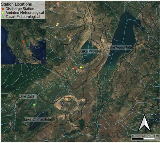
Figure 1. Satellite map of the study area in Western Macedonia, Northern Greece, showing the interconnected lake system (Zazari, Chimaditida, Petron, Vegoritida) and the location of the hydrological monitoring station (red dot), along with two additional meteorological stations (yellow and green dots). Blue lines represent the delineated stream network derived from the DEM, while black lines outline the watershed boundaries. This spatial overview highlights the flow path and key hydrological features considered in the hybrid modeling framework.

Hydrologically, the system follows a connected lake sequence. Overflow from Lake Zazari is directed into Lake Chimaditida through a connecting canal. When Lake Chimaditida reaches capacity, excess water is discharged via a small overflow structure into the main drainage ditch, which serves both irrigation and flood control purposes. The area is influenced not only by natural rainfall–runoff processes but also by irrigation return flows and water management infrastructure, similar to other agricultural regions in Western Macedonia [8]. Along this ditch, near the village of Rodonas, part of the water is temporarily stored or diverted for agricultural use. The hydrological monitoring station used in this study is positioned just downstream of these inflows, providing a representative measurement of the combined natural and anthropogenic contributions before the water continues toward Lake Petron.

Climatically, the region exhibits a Mediterranean continental pattern, with wet winters and dry summers. Annual precipitation ranges from 550 to 600 mm, with the bulk occurring between October and April, while the summer months are typically dry and characterized by peak irrigation activity.

Temperature varies widely throughout the year, with winter lows frequently below 0 °C and summer highs exceeding 30 °C. These seasonal dynamics are visualized in Figure 2, which presents an ombrothermic diagram summarizing the monthly distribution of temperature and precipitation.

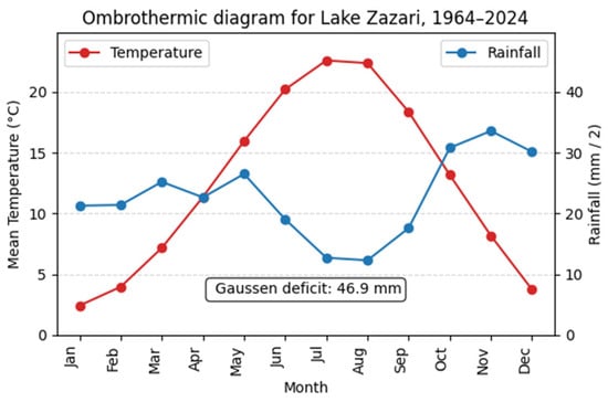
Figure 2. Ombrothermic diagram for Lake Zazari (1967–2024), illustrating the monthly mean temperature (red line) and half the monthly precipitation (blue line). The summer months show a pronounced climatic water deficit (deficit: 46.90), indicating a dry period with high evapotranspiration demand relative to rainfall—a key consideration for irrigation management in the study area. Note: Rainfall values are divided by 2 to match scale with temperature (as per Gaussens’s method).

3.1.2. Meteorological Data

The study analyzed the meteorological data obtained from the network of agrometeorological stations of Prefecture Florina, Western Macedonia. Meteorological variables were collected from the station of Aminteo, while precipitation data were also included from a station near lake Zazari. The meteorological variables include air temperature and rainfall, while wind speed solar radiation and relative humidity were also processed to calculate evapotranspiration. Figure 3 depicts temperature and precipitation data used in this study. The availability of high-resolution radiation and sunshine data in the area enabled improved modeling of evapotranspiration and energy balance [41,42]. For this study, reference crop evapotranspiration was calculated using the Penman–Monteith formula [43] (Figure 4).

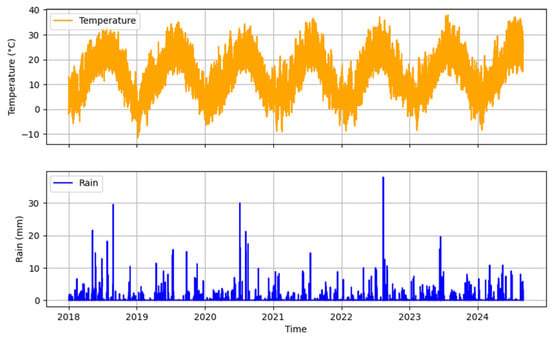
Figure 3. Time series of meteorological conditions (air temperature (top) and precipitation (bottom)) in the study area (2018–2024).

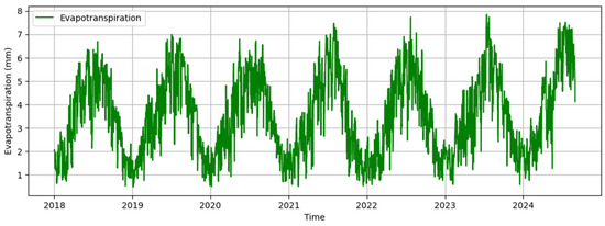
Figure 4. Daily time series of evapotranspiration (mm) from 2018 to 2024 in the study area.

3.1.3. Hydrological Data

Hydrological data include water level (stage height) measurements obtained from a monitoring station located at 40°41′46.1″ N, 21°39′48.2″ E. The station is equipped with an ultrasound sensor capable of recording water level data at a 10-min interval temporal resolution that were aggregated to hourly resolution. Figure 5 depicts the two monitoring stations used in this study.

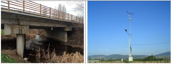
Figure 5. (Left) Hydrological monitoring station located under a bridge in the study area. (Right) Meteorological station used for collecting weather data including temperature, precipitation, wind speed, and solar radiation.

Since direct discharge measurements were not available; streamflow was estimated using an empirical stage–discharge relationship:

Q = a h^b

where Q is the discharge (in m³/s), h is the stage height (in meters), and the parameters a = 0.00009 and b = 2.2203 were fitted based on multi-year field measurements provided by the regional water management authority.

The resulting discharge time series spanned the period from 1 January 2018 to 1 September 2024 (Greek local time) capturing both high- and low-flow conditions. Standard preprocessing steps were applied to remove outliers and fill any missing values through linear interpolation. These data points were used for both training and evaluation of the proposed hybrid forecasting framework.

Figure 6 visualizes the standard deviation of the hourly discharge on daily, weekly, and monthly bases. These metrics show how variability evolves over time at different resolutions.

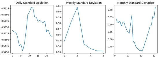
Figure 6. Standard deviation of streamflow values at different temporal resolutions: (left) daily, (center) weekly, and (right) monthly.

3.2. Framework Overview

Accurately forecasting streamflow remains a significant challenge in hydrology, particularly due to complexities introduced by human interventions such as irrigation, which are often inadequately represented in conventional physical models. The objective of this study is to investigate a hybrid modeling framework that integrates physically based hydrological simulations with deep learning techniques to enhance streamflow prediction accuracy and reliability, particularly addressing biases arising from human irrigation practices.

Figure 7 demonstrates the processes of the hybrid framework. Initially, the Hydrologic Engineering Center’s Hydrologic Modeling System (HEC-HMS) was utilized to generate synthetic streamflow data. This model integrated meteorological data and watershed characteristics derived from a Digital Elevation Model (DEM), generating physically consistent discharge simulations across the catchment.

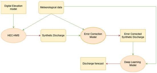
Figure 7. Overview of the hybrid streamflow forecasting framework. The process integrates digital elevation and meteorological data into the HEC-HMS model to generate synthetic discharge, which is then corrected using an error correction model. The corrected discharge is used as input to a deep learning model for discharge forecasting.

Recognizing that the synthetic discharge generated by HEC-HMS does not inherently account for irrigation-induced streamflow alterations, a dedicated bias correction model was employed. This model learns systematic discrepancies between the physically simulated and observed discharge data attributable to irrigation withdrawals or returns. By correcting these biases, the resulting synthetic discharge data more closely mirror observed flow patterns that reflect actual human management practices within the watershed.

Finally, the bias-corrected synthetic discharge serves as input into a deep learning model—specifically, a Temporal Fusion Transformer (TFT)—alongside additional meteorological data and temporal variables to predict real observed streamflow. By combining physically informed bias-corrected synthetic data with data-driven predictive capabilities, this stage effectively leverages the strengths of both physical and deep learning modeling approaches.

For both the bias correction and deep learning stages, the available discharge time series was partitioned using a temporal split, with 80% allocated for training and 20% held out for validation. The validation period spanned from 1 September 2023 to 1 September 2024, covering a full hydrological year and capturing seasonal variability, including both irrigation and non-irrigation periods. This split ensured a realistic evaluation of model generalization under diverse flow conditions while maintaining chronological integrity to avoid data leakage.

To assess the robustness of our training setup, we compared two sampling strategies: (i) non-overlapping windows, where input–output sequences were spaced apart to avoid redundancy, and (ii) overlapping windows, where the sliding window advanced one timestep at a time. Both approaches produced consistent performance, confirming the stability of the model. These components are described in detail in Section 3.2.1, Section 3.2.2, Section 3.2.3.

3.2.1. Physical Model

The physically based component of the hybrid framework was implemented using HEC-HMS (Hydrologic Engineering Center’s Hydrologic Modeling System). The model was configured to simulate streamflow for the selected catchment based on sub-basin delineation derived from a high-resolution Digital Elevation Model (DEM) combined with hourly meteorological inputs, including precipitation and temperature.

The watershed delineation was based on the HydroSHEDS [44] void-filled digital elevation model at 15 arc-second resolution. The stream network was defined using the Copernicus Land Monitoring Service’s European River Network Database [45], which provided accurate reach delineation for the interconnected lake system. The HEC-HMS built-in GIS tools were used for terrain preprocessing, including terrain reconditioning, sink treatment, drainage preprocessing, and stream network identification.

Standard modeling components were employed, including the SCS Curve Number method [46] for surface runoff estimation, the Clark Unit Hydrograph [47] for transform modeling, and Muskingum routing for channel flow [48]. The model was run at an hourly timesteps to capture short-term hydrological dynamics relevant for discharge forecasting.

The meteorological model incorporated rainfall data from spatially distributed weather stations located in Zazari and Amyntaio to account for precipitation variability across the watershed’s sub-basins. Additionally, air temperature, wind speed, relative humidity, and evapotranspiration from Amyntaio station were given as inputs (see Section 2.2).

Model calibration was performed using observed discharge data from the basin outlet over a yearlong period. Calibration focused on minimizing discrepancies between observed and simulated discharge using performance metrics such as the Nash–Sutcliffe Efficiency (NSE) and the Kling–Gupta Efficiency (KGE) [49,50]. While the model was effective in capturing general runoff trends, discrepancies were noted during irrigation periods, particularly during dry seasons—highlighting the need for subsequent bias correction.

Importantly, irrigation activities and other anthropogenic influences were not explicitly modeled in HEC-HMS, and their absence is addressed in the next stage of the framework through a data-driven correction process.

3.2.2. Bias Correction Model

While physically based models are effective at simulating natural hydrological processes such as rainfall–runoff generation and streamflow routing, many of them (such as HEC-HMS used in this study) do not account for human behaviors, such as water withdrawals for irrigation. In agricultural regions, particularly during summer months, farmers often extract significant amounts of water—sometimes through unregulated or informal practices—that alter streamflow in ways the physical model cannot represent. As a result, the discrepancy between simulated and observed discharge is not merely a modeling error but reflects real, unmodeled human influence.

To address systematic errors introduced by unmodeled human activities, a bias correction model was developed to adjust the synthetic streamflow outputs from HEC-HMS. The correction approach is based on supervised learning, wherein the error between observed and simulated discharge (i.e., residuals) is predicted using a multi-layer perceptron (MLP) regressor.

The bias correction model utilizes a set of temporal and seasonal features—such as hour, day, month, and one-hot encoded seasons—as inputs, capturing faulty periodic behavior across the year. The model was trained using a sub-set of the training data, specifically targeting the months from July through November, when irrigation activity is most pronounced. This focused training set allowed it to specifically focus on correcting irrigation-driven deviations that are not captured by the physical model.

The trained MLP model demonstrated strong predictive capability on held-out test data, and its predictions were used to adjust the raw HEC-HMS outputs. Specifically, the predicted error was added to the simulated discharge to produce a corrected streamflow series. Performance was evaluated using standard hydrological metrics such as the Nash–Sutcliffe Efficiency (NSE), modified Kling–Gupta Efficiency (KGE), and RMSE, all of which indicated improved alignment with observed discharge during both calibration and validation periods.

3.2.3. Deep Learning Model

This study employed the Temporal Fusion Transformer (TFT) architecture, following the same configuration as used in our previous work [34], where it demonstrated superior performance in short-term water level forecasting. Given its effectiveness in capturing complex temporal relationships and its capacity for interpretable multi-step prediction, the TFT was selected as the deep learning component of our hybrid framework.

To formally define the problem and improve mathematical clarity, we now briefly present the core equations of the Temporal Fusion Transformer (TFT) components as applied in this study. These include the input–output structure, gated residual networks (GRNs), multi-head attention, and LSTM layers.

At timestep $t$ for a forecast horizon of length H, we aim to predict target $y_{t+\tau }\in R$ for all timesteps $\mathsf{\tau }\in \{1, \dots , H\},$ given a set of input feature variables. Input features are divided into observed inputs $z_t$, which are only available up to the present timestep $t$ and known future inputs $x_t$ which can be predetermined for timesteps $t+1, \dots , t+H$. To condition forecasts on recent dynamics, we use a fixed-length lookback window of size $k$, which provides the model with access to the most recent $k$ historical values of the target and covariates ($t-k$ timesteps). As such, we adopt quantile regression to our multi-horizon forecasting setting. Each quantile forecast takes the form

$$\widehat{y^{\left(q\right)}}\left(t,\mathsf{\tau }\right)={ TFT}_q\left(\mathsf{\tau },\hspace{0.17em}{y}_{t-k:t},\hspace{0.17em}{z}_{t-k:t},\hspace{0.17em}{x}_{t-k:t+\mathsf{\tau }}\right)$$

where $\widehat{y^{\left(q\right)}}\left(t,\tau \right)$ denotes the TFT model’s estimate of the $q$-th conditional quantile of the future target value ${\mathrm{y}}_{\mathrm{t}+\mathsf{\tau }}$ for a forecast horizon $\tau$, given all available information up to time t and known future inputs up to time $t+\mathsf{\tau }$.

To capture temporal dynamics, the TFT employs a sequence-to-sequence LSTM architecture. The encoder processes past observed and known inputs within a fixed lookback window, generating hidden and cell states that summarize the recent sequence. These states are then used to initialize the LSTM decoder, which processes known future inputs. This results in a temporally aware representation that serves as the foundation for downstream processing by the attention and gating components.

To refine the extracted temporal features, TFT applies gated residual networks (GRNs). The information flow through the GRNs can be represented using the following equations:

$$\begin{array}{l}\mathrm{GRN}\left(a\right)= \mathrm{L}\mathrm{a}\mathrm{y}\mathrm{e}\mathrm{r}\mathrm{N}\mathrm{o}\mathrm{r}\mathrm{m} \left(a+GLU\left({\eta }_1\right)\right)\\ GLU\left({\eta }_1\right)=\sigma \left(W_1{\eta }_1+b_1\right)\odot \left(W_2{\eta }_1+b_2\right)\\ {\eta }_1={ W}_3{\eta }_2+b_3\\ {\eta }_2=ELU\left(W_{4}a+b_4\right)\end{array}$$

Here, $a$ is the basic input to GRN, and $W$ and $b$ are weights and biases that are optimized during training. Firstly, $a$ passes through a dense layer with Exponential Linear Unit (ELU) activation function [51], followed by a linear layer with dropout. The output from this layer goes into a Gated Linear Unit [52], where ⊙ is the element-wise product, and σ is the sigmoid activation function. Finally, the output from GRN is calculated by standard layer normalization of the sum of input $a$ and GLU output (residual connection).

Following temporal encoding and gating, the model employs an interpretable multi-head attention mechanism to capture long-range dependencies across the input sequence. Unlike standard attention, TFT’s modified design shares value projections across all heads and uses additive aggregation to combine their outputs.

$$\begin{array}{l} \mathrm{M}\mathrm{u}\mathrm{l}\mathrm{t}\mathrm{i}\mathrm{H}\mathrm{e}\mathrm{a}\mathrm{d} \left(Q,K,V\right)=\left[H_1,\dots ,H_{m_H}\right]W_H\\ H_h= \mathrm{A}\mathrm{t}\mathrm{t}\mathrm{e}\mathrm{n}\mathrm{t}\mathrm{i}\mathrm{o}\mathrm{n} \left(Q{W}_Q^{\left(h\right)},K{W}_K^{\left(h\right)},V{W}_V^{\left(h\right)}\right)\\ \mathrm{T}\mathrm{T}\mathrm{F}\mathrm{M}\mathrm{u}\mathrm{l}\mathrm{t}\mathrm{i}\mathrm{H}\mathrm{e}\mathrm{a}\mathrm{d} (Q,K,V)=\overline{H}{W}_H\\ \overline{H}=\overline{A}(Q,K)V{W}_V=1/H{\displaystyle \sum _{h=1}^{m_H}} \mathrm{A}\mathrm{t}\mathrm{t}\mathrm{e}\mathrm{n}\mathrm{t}\mathrm{i}\mathrm{o}\mathrm{n} \left(Q{W}_Q^{\left(h\right)},K{W}_K^{\left(h\right)},V{W}_V^{\left(h\right)}\right)\end{array}$$

where $Q, K, V$ are the standard attention query, key, and value matrices, $W_V$ values are value weights shared across all heads, and $W_H$ is used for the final linear mapping. This helps each head to learn different temporal patterns while attending a common set of input features.

In this setting, the model was trained to generate 24-h-ahead forecasts of observed discharge, using a lookback window of 24 h of bias-corrected synthetic discharge along with relevant meteorological covariates. These include air temperature, precipitation, relative humidity, wind speed, and potential evapotranspiration—variables that reflect both short-term weather conditions and broader water balance dynamics.

To evaluate longer forecast horizons, the TFT was retrained using 48-h and 72-h multi-output configurations. This allowed direct comparison across multiple time horizons without the compounding error typical in autoregressive rollouts.

The implementation and configuration of the model followed those detailed in Ampas and Refanidis (2024) [34], which served as the primary reference for both the architectural setup and training procedure used in this work. For completeness, we note that the Temporal Fusion Transformer (TFT) model employed here used 100 hidden units for a single recurrent layer and 4 attention heads. A dropout rate of 0.01 was applied to improve generalization. The learning rate was optimized using the Optuna hyperparameter tuning framework [53]. In terms of input features, the model leveraged not only meteorological and discharge variables but also lagged water level values at 12 and 24 h and accumulated precipitation from multiple stations across the watershed. Temporal features, including hour, month, and season (encoded as dummy variables), were treated as known future covariates to support real-world applicability and enhance the model’s temporal context.

4. Results and Discussion

4.1. Performance of the Bias Correction Model

The multi-layer perceptron (MLP) bias correction model was trained using data from months with intensive irrigation activity (July through November). Once trained, the model’s predicted error was reapplied across the full synthetic discharge series, effectively integrating the learned corrections into the HEC-HMS output. This produced a complete, bias-corrected streamflow time series, which was then used in both the training and validation phases of the deep learning model.

The bias correction demonstrated strong improvements across multiple performance metrics. Specifically, on the calibration dataset, the Nash–Sutcliffe Efficiency (NSE) increased from an initial 0.52 (raw HEC-HMS output) to 0.84 after correction, the Kling–Gupta Efficiency (KGE) improved from 0.65 to 0.90, and the R-squared value rose from 0.56 to 0.88. The validation dataset results similarly indicated substantial performance gains (NSE = 0.82, KGE = 0.88, R-squared = 0.85).

The full time series (including calibration and validation periods combined) demonstrated robust performance (NSE = 0.83, KGE = 0.89, R-squared = 0.86), indicating that the bias-corrected synthetic discharge closely resembles the observed discharge patterns, effectively capturing human irrigation impacts (Figure 8). These results confirm that the corrected synthetic discharge provides a reliable and realistic input dataset for subsequent deep learning modeling.

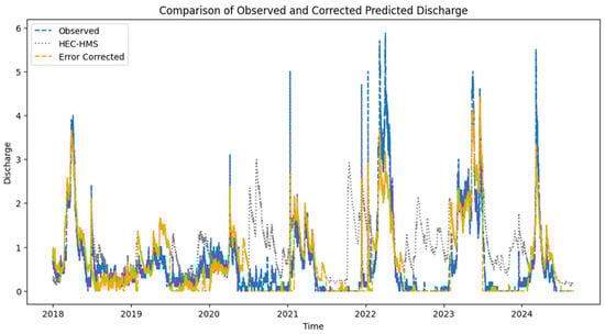
Figure 8. Comparison of observed discharge, HEC-HMS simulated discharge, and bias-corrected discharge for the period 2018–2024. The plot highlights improvements in alignment between corrected predictions and observed values following error correction.

4.2. Deep Learning Model Forecasting Performance

The Temporal Fusion Transformer (TFT) model, trained using the bias-corrected synthetic discharge as its primary input, exhibited strong predictive performance and interpretability. Table 2 summarizes its point-forecast performance alongside two benchmarks: raw (uncorrected) synthetic discharge inputs and an “ideal” model trained directly on observed discharge. For the 24-h horizon, the TFT achieved an NSE of 0.84, KGE of 0.89, and RMSE of 0.301 m³/s, substantially outperforming the uncorrected input model (NSE = 0.55, KGE = 0.67, RMSE = 1.084 m³/s) and approaching the observed-input case (NSE = 0.90, KGE = 0.92, RMSE = 0.247 m³/s) Our model’s performance is comparable to our previous work [34], where the TFT was benchmarked against other models (NSE= 0.9234, KGE= 0.9585) as well as against results reported in similar studies, as summarized in Table 1. (e.g., NSE = 0.78–0.99, KGE ≈ 0.70–0.90),

Table 2. Comparison of streamflow forecast accuracy using different model input types. Performance metrics include Nash–Sutcliffe Efficiency (NSE), Kling–Gupta Efficiency (KGE), and Root Mean Square Error (RMSE). The bias-corrected synthetic discharge shows improved performance over raw synthetic inputs and approaches the accuracy of forecasts based on observed discharge.

Model Input Type	NSE	KGE	RMSE
Raw Synthetic Discharge (uncorrected)	0.55	0.67	1.084
Bias-corrected Synthetic Discharge	0.84	0.89	0.301
Observed Discharge (ideal case)	0.90	0.92	0.247

The results clearly indicate that the bias-corrected synthetic discharge enhances predictive performance compared to uncorrected synthetic inputs, closely approaching the ideal scenario using observed discharge data. This indicates that the proposed hybrid approach successfully bridges the gap between purely synthetic and observed data-driven forecasting methods.

Table 3 presents the predictive performance of the proposed hybrid model across 24-, 48-, and 72-h forecast horizons. As expected, the model accuracy exhibited a gradual decline with increasing lead time. For the 24-h horizon, the model achieved strong performance, with an NSE of 0.84 and KGE of 0.89, indicating high reliability in short-term forecasting. The root mean square error (RMSE) remained low at 0.301 m³/s.

Table 3. Forecast performance of the hybrid model across different lead times. Evaluation metrics are presented for 24-, 48-, and 72-h forecast horizons using the Temporal Fusion Transformer (TFT). A gradual decline in accuracy with increasing lead time is observed.

Forecast Horizon	NSE	KGE	RMSE
24 h ahead	0.84	0.89	0.301
48 h ahead	0.78	0.79	0.743
72 h ahead	0.71	0.74	0.980

At 48 and 72 h, the model retained reasonable skill, with the NSE and KGE remaining above 0.70 at both horizons. This gradual performance degradation is expected in multi-step forecasting tasks.

An important advantage of the TFT is its built-in probabilistic forecasting. As shown in Table 4, the mean Continuous Ranked Probability Score (CRPS) improved from 0.155 to 0.074 m³/s after bias correction, while the empirical coverage rates for the 60%, 80%, and 98% predictive intervals rose from 52.2%, 71.2%, and 89.4% (raw inputs) to 63.4%, 79.1%, and 96.6% (bias-corrected inputs), respectively. The close alignment between the nominal and empirical coverage confirms that the TFT is capable of producing reliable uncertainty bounds, which is a critical feature for water management.

Table 4. Probabilistic forecast performance using different input types. Metrics include Continuous Ranked Probability Score (CRPS) and empirical coverage percentages for 60%, 80%, and 98% prediction intervals. The bias-corrected inputs yielded improved reliability and uncertainty quantification.

Model Input Type	Mean CRPS	60% cov.	80% cov.	98% cov.
Raw Synthetic Discharge (uncorrected)	0.615	0.522	0.712	0.894
Bias-corrected Synthetic Discharge	0.174	0.634	0.791	0.966
Observed Discharge (ideal case)	0.151	0.621	0.806	0.974

Furthermore, temporal and seasonal attention weights from the TFT model provided valuable insights into the relative importance of various input variables (Figure 9). The corrected synthetic discharge was consistently the highest weighted input feature, confirming its critical role in predictive performance. The precipitation and evapotranspiration-related variables also contributed meaningfully, highlighting the model’s responsiveness to short-term meteorological drivers.

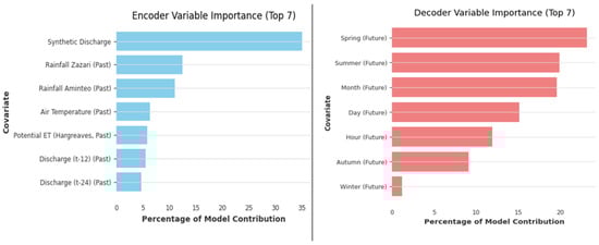
Figure 9. Variable importance for the Temporal Fusion Transformer model. (Left) Top encoder input variables, with synthetic discharge and rainfall variables contributing most to the model. (Right) Top decoder input variables, highlighting seasonal and temporal features influencing forecast output.

Decoder importance was led by seasonal indicators such as spring and summer, aligning with periods of intensive irrigation activity. This suggests that the model effectively captures recurring human-induced flow alterations without requiring explicit irrigation inputs, further supporting its utility in semi-arid, agriculture-driven watersheds.

In addition to variable importance, the attention heat map (Figure 10) offers a temporal perspective on how the model distributes focus across the input sequence. The highest attention weights are concentrated around the most recent timesteps just before the forecast window, indicating the model’s reliance on immediate past conditions for making near-term predictions. As the temporal distance increases, attention diminishes—suggesting that older inputs carry less predictive influence. This pattern reflects the short-memory behavior typical in streamflow dynamics and reinforces the model’s responsiveness to recent fluctuations in discharge and weather conditions.

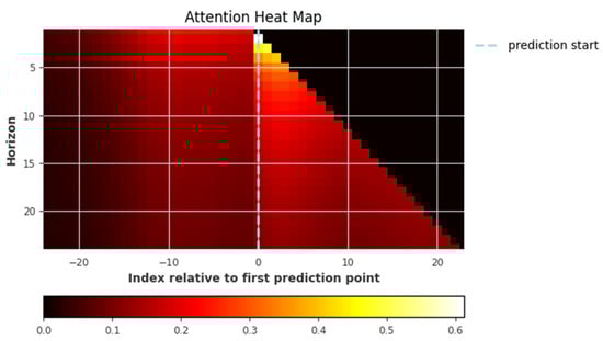
Figure 10. Variable attention heat map from the Temporal Fusion Transformer model. The plot illustrates how the model allocates attention across the input sequence relative to the prediction window. Warmer colors indicate higher attention weights, with the strongest focus placed on timesteps immediately preceding the forecast start.

These findings underscore the operational potential of the hybrid modeling approach, particularly in scenarios where direct observations are unavailable or incomplete. The model’s reliable performance, combined with interpretability through feature importance, positions it as a valuable tool for operational forecasting, particularly in real-time applications or ungauged basins where synthetic inputs are often the only feasible source of continuous data.

4.3. Operational and Generalization Potential

The proposed hybrid modeling framework demonstrates practical advantages. Its reliance on corrected synthetic discharge inputs significantly reduces dependence on real-time sensor data, ensuring continuity and robustness during sensor failures, equipment maintenance, or data collection gaps. This capability is particularly valuable in operational settings, facilitating consistent and reliable forecasting that supports informed decision making in real-time applications.

The modular nature of this framework enhances its flexibility, allowing independent adjustment. Each component—the physical hydrological model, the bias correction method, and the deep learning prediction model—can be individually adjusted or replaced, offering water managers flexibility in adapting the framework to local conditions and available resources. This modularity not only improves interpretability but also supports straightforward adaptation and application across diverse geographic and management contexts.

4.4. Limitations and Future Directions

While the hybrid modeling framework shows strong potential, several limitations should be noted. The approach depends heavily on the accuracy of the physical model (HEC-HMS), and performance may degrade if the model is poorly calibrated. The bias correction mechanism is tailored to a specific region and seasonal irrigation behavior, which may limit its transferability. This study is limited to a single discharge point; however, the proposed framework could be extended to spatially distributed streamflow forecasting by incorporating sub-watershed delineation or multi-point calibration where data availability permits.

Future work should focus on scaling the framework to larger, multi-basin datasets and developing a generalized, foundational deep learning model trained across diverse hydrological regimes. Integrating additional data sources—such as remote sensing, land use, canopy evapotranspiration, irrigation records, and high-resolution forecasts—can further enrich the input space. Ultimately, automating the full pipeline and validating it across multiple regions could pave the way for a scalable, operational forecasting system suitable for real-time deployment, especially in ungauged or data-scarce basins.

5. Conclusions

This study introduced a hybrid hydrological forecasting framework that integrates physically based modeling (HEC-HMS), machine learning-based bias correction, and a Temporal Fusion Transformer (TFT) to generate accurate, multi-horizon streamflow predictions in a semi-arid, irrigation-impacted basin in Northern Greece.

By correcting irrigation-induced discrepancies in synthetic discharge data, the proposed framework significantly improved forecast accuracy, with an NSE increasing from 0.55 to 0.84 and an RMSE decreasing from 1.084 to 0.301 m³/s. When used as input to the TFT, the bias-corrected data enabled robust 24-, 48-, and 72-h streamflow forecasts with high reliability and well-calibrated uncertainty bounds. The model’s interpretability further uncovered key temporal and meteorological drivers, such as seasonal irrigation patterns and rainfall events, contributing to both scientific insight and operational transparency.

Despite relying primarily on synthetic inputs, the hybrid model achieved performance comparable to observed-data-driven baselines. Its modular design—separating physical simulation, bias correction, and deep learning—allows for flexible adaptation across different basins and data availability levels. This makes the framework particularly suitable for ungauged or data-scarce environments, where conventional monitoring may fall short.

Overall, this work demonstrates that combining the physical realism of hydrological simulation with the pattern recognition capabilities of deep learning leads to reliable, explainable, and transferable streamflow forecasts. Future research should explore scaling this approach to larger catchments, automating data ingestion pipelines, and incorporating diverse data sources to further enhance performance and generalizability.

References

- de Oliveira, C.M. Sustainable access to safe drinking water: Fundamental human right in the international and national scene. Rev. Ambiente Água 2017, 12, 985–1000. [Google Scholar] [CrossRef]
- UNGA Resolution. Resolution A/RES/64/292: The Human Right to Water and Sanitation; United Nations: New York, NY, USA, 2010. [Google Scholar]
- Guo, Y.; Li, P.; He, X.; Wang, L. Groundwater Quality in and Around a Landfill in Northwest China: Characteristic Pollutant Identification, Health Risk Assessment, and Controlling Factor Analysis. Expo. Health 2022, 14, 885–901. [Google Scholar] [CrossRef]
- Khan, M.H.; Nafees, M.; Muhammad, N.; Ullah, U.; Hussain, R.; Bilal, M. Assessment of Drinking Water Sources for Water Quality, Human Health Risks, and Pollution Sources: A Case Study of the District Bajaur, Pakistan. Arch. Environ. Contam. Toxicol. 2021, 80, 41–54. [Google Scholar] [CrossRef] [PubMed]
- Huang, F.; Wang, G.H.; Yang, Y.Y.; Wang, C.B. Overexploitation status of groundwater and induced geological hazards in China. Nat. Hazards 2014, 73, 727–741. [Google Scholar] [CrossRef]
- Wu, J.; Li, P.; Qian, H.; Fang, Y. Assessment of soil salinization based on a low-cost method and its influencing factors in a semi-arid agricultural area, northwest China. Environ. Earth Sci. 2014, 71, 3465–3475. [Google Scholar] [CrossRef]
- van Emmerik, T.; Mulder, G.; Eilander, D.; Piet, M.; Savenije, H. Predicting the ungauged basin: Model validation and realism assessment. Front. Earth Sci. 2015, 3, 62. [Google Scholar] [CrossRef]
- Ragkos, A.; Ambas, V. Examining the potential of an irrigation work to improve sustainability in a rural area. Water Supply 2021, 21, 2959–2973. [Google Scholar] [CrossRef]
- Coulibaly, S.; Kamsu-Foguem, B.; Kamissoko, D.; Traore, D. Deep learning for precision agriculture: A bibliometric analysis. Intell. Syst. Appl. 2022, 16, 200102. [Google Scholar] [CrossRef]
- Jain, S.K.; Mani, P.; Prakash, P.; Singh, V.P.; Tullos, D.; Kumar, S.; Agarwal, S.P.; Dimri, A.P. A Brief review of flood forecasting techniques and their applications. Int. J. River Basin Manag. 2018, 16, 329–344. [Google Scholar] [CrossRef]
- Beven, K. Data for Rainfall–Runoff Modelling. In Rainfall-Runoff Modelling; John Wiley & Sons, Ltd.: Hoboken, NJ, USA, 2012; pp. 51–82. [Google Scholar] [CrossRef]
- Rolnick, D.; Donti, P.L.; Kaack, L.H.; Kochanski, K.; Lacoste, A.; Sankaran, K.; Ross, A.S.; Milojevic-Dupont, N.; Jaques, N.; Waldman-Brown, A.; et al. Tackling Climate Change with Machine Learning. ACM Comput. Surv. 2022, 55, 1–96. [Google Scholar] [CrossRef]
- Karyotis, K.; Tziolas, N.; Tsakiridis, N.; Chatzimisios, P.; Kontoes, C.; Zalidis, G. A Multi-layered Convolutional Neural Network for Soil Variables Estimation with the Combination of Open Access Data. In Selected Studies in Geotechnics, Geo-informatics and Remote Sensing; Ergüler, Z.A., Hadji, R., Chaminé, H.I., Rodrigo-Comino, J., Kallel, A., Merkel, B., Eshagh, M., Chenchouni, H., Grab, S., Karakus, M., et al., Eds.; Springer Nature: Cham, Switzerland, 2023; pp. 129–135. [Google Scholar] [CrossRef]
- Tsakiridis, N.L.; Chadoulos, C.G.; Theocharis, J.B.; Ben-Dor, E.; Zalidis, G.C. A three-level Multiple-Kernel Learning approach for soil spectral analysis. Neurocomputing 2020, 389, 27–41. [Google Scholar] [CrossRef]
- Kalopesa, E.; Karyotis, K.; Tziolas, N.; Tsakiridis, N.; Samarinas, N.; Zalidis, G. Estimation of Sugar Content in Wine Grapes via In Situ VNIR–SWIR Point Spectroscopy Using Explainable Artificial Intelligence Techniques. Sensors 2023, 23, 1065. [Google Scholar] [CrossRef] [PubMed]
- Karyotis, K.-V.; Gülbahar, N.; Panagopoulos, A. A Two-Dimensional Nitrogen Fertilization Model for Irrigated Crops in Turkey. Am. Sci. Res. J. Eng. Technol. Sci. 2018, 41, 319–332. [Google Scholar]
- Arsenault, R.; Martel, J.-L.; Brunet, F.; Brissette, F.; Mai, J. Continuous streamflow prediction in ungauged basins: Long short-term memory neural networks clearly outperform traditional hydrological models. Hydrol. Earth Syst. Sci. 2023, 27, 139–157. [Google Scholar] [CrossRef]
- Hestness, J.; Narang, S.; Ardalani, N.; Diamos, G.; Jun, H.; Kianinejad, H.; Patwary, M.A.; Yang, Y.; Zhou, Y. Deep Learning Scaling is Predictable, Empirically. arXiv 2017, arXiv:1712.00409. [Google Scholar] [CrossRef]
- Kratzert, F.; Klotz, D.; Brenner, C.; Schulz, K.; Herrnegger, M. Rainfall–runoff modelling using Long Short-Term Memory (LSTM) networks. Hydrol. Earth Syst. Sci. 2018, 22, 6005–6022. [Google Scholar] [CrossRef]
- Nearing, G.S.; Kratzert, F.; Sampson, A.K.; Pelissier, C.S.; Klotz, D.; Frame, J.M.; Prieto, C.; Gupta, H.V. What Role Does Hydrological Science Play in the Age of Machine Learning? Water Resour. Res. 2021, 57, e2020WR028091. [Google Scholar] [CrossRef]
- Dehghani, A.; Moazam, H.M.Z.H.; Mortazavizadeh, F.; Ranjbar, V.; Mirzaei, M.; Mortezavi, S.; Ng, J.L.; Dehghani, A. Comparative evaluation of LSTM, CNN, and ConvLSTM for hourly short-term streamflow forecasting using deep learning approaches. Ecol. Inform. 2023, 75, 102119. [Google Scholar] [CrossRef]
- Ostadkalayeh, F.B.; Moradi, S.; Asadi, A.; Nia, A.M.; Taheri, S. Performance Improvement of LSTM-based Deep Learning Model for Streamflow Forecasting Using Kalman Filtering. Water Resour. Manag. 2023, 37, 3111–3127. [Google Scholar] [CrossRef]
- Lin, Y.; Wang, D.; Wang, G.; Qiu, J.; Long, K.; Du, Y.; Xie, H.; Wei, Z.; Shangguan, W.; Dai, Y. A hybrid deep learning algorithm and its application to streamflow prediction. J. Hydrol. 2021, 601, 126636. [Google Scholar] [CrossRef]
- Wegayehu, E.B.; Muluneh, F.B. Short-Term Daily Univariate Streamflow Forecasting Using Deep Learning Models. Adv. Meteorol. 2022, 2022, 1860460. [Google Scholar] [CrossRef]
- Farfán-Durán, J.F.; Cea, L. Streamflow forecasting with deep learning models: A side-by-side comparison in Northwest Spain. Earth Sci. Inform. 2024, 17, 5289–5315. [Google Scholar] [CrossRef]
- Burrichter, B.; da Silva, J.K.; Niemann, A.; Quirmbach, M. A Temporal Fusion Transformer Model to Forecast Overflow from Sewer Manholes during Pluvial Flash Flood Events. Hydrology 2024, 11, 41. [Google Scholar] [CrossRef]
- Koya, S.R.; Roy, T. Temporal Fusion Transformers for streamflow Prediction: Value of combining attention with recurrence. J. Hydrol. 2024, 637, 131301. [Google Scholar] [CrossRef]
- Neisary, S.N.; Johnson, R.C.; Alam, S.; Burian, S.J. A Post-Processing Machine Learning Framework for Bias-Correcting National Water Model Outputs by Accounting for Dominant Streamflow Drivers. Environ. Model. Softw. 2025, 190, 106459. [Google Scholar] [CrossRef]
- Liu, S.; Wang, J.; Wang, H.; Wu, Y. Post-processing of hydrological model simulations using the convolutional neural network and support vector regression. Hydrol. Res. 2022, 53, 605–621. [Google Scholar] [CrossRef]
- Lim, B.; Arık, S.Ö.; Loeff, N.; Pfister, T. Temporal Fusion Transformers for interpretable multi-horizon time series forecasting. Int. J. Forecast. 2021, 37, 1748–1764. [Google Scholar] [CrossRef]
- Zhou, R.; Wang, Q.; Jin, A.; Shi, W.; Liu, S. Interpretable multi-step hybrid deep learning model for karst spring discharge prediction: Integrating temporal fusion transformers with ensemble empirical mode decomposition. J. Hydrol. 2024, 645, 132235. [Google Scholar] [CrossRef]
- Francisco, R.; Matos, J.P.; Marinheiro, R.; Lopes, N.; Portela, M.M.; Barros, P. Application of Temporal Fusion Transformers to Run-Of-The-River Hydropower Scheduling. Hydrology 2025, 12, 81. [Google Scholar] [CrossRef]
- Huang, F.; Ochoa, C.G.; Li, Q.; Shen, X.; Qian, Z.; Han, S.; Zhang, N.; Yu, M. Forecasting environmental water availability of lakes using temporal fusion transformer: Case studies of China’s two largest freshwater lakes. Environ. Monit. Assess. 2024, 196, 152. [Google Scholar] [CrossRef]
- Ampas, T.; Refanidis, I. Leveraging deep learning methods to enhance hydrological predictions and model interpretability. In SETN ’24, Proceedings of the 13th Hellenic Conference on Artificial Intelligence, Piraeus, Greece, 11–13 September 2024; Association for Computing Machinery: New York, NY, USA, 2024; pp. 1–6. [Google Scholar] [CrossRef]
- Kumar, S.; Choudhary, M.K.; Thomas, T. A hybrid technique to enhance the rainfall-runoff prediction of physical and data-driven model: A case study of Upper Narmada River Sub-basin, India. Sci. Rep. 2024, 14, 26263. [Google Scholar] [CrossRef] [PubMed]
- Difi, S.; Heddam, S.; Zerouali, B.; Kim, S.; Elmeddahi, Y.; Bailek, N.; Santos, C.A.G.; Abida, H. Improved daily streamflow forecasting for semi-arid environments using hybrid machine learning and multi-scale analysis techniques. J. Hydroinform. 2024, 26, 3266–3286. [Google Scholar] [CrossRef]
- Samarinas, N.; Tziolas, N.; Zalidis, G. Improved Estimations of Nitrate and Sediment Concentrations Based on SWAT Simulations and Annual Updated Land Cover Products from a Deep Learning Classification Algorithm. ISPRS Int. J. Geo-Information 2020, 9, 576. [Google Scholar] [CrossRef]
- Lin, Y.; Wang, D.; Meng, Y.; Sun, W.; Qiu, J.; Shangguan, W.; Cai, J.; Kim, Y.; Dai, Y. Bias learning improves data driven models for streamflow prediction. J. Hydrol. Reg. Stud. 2023, 50, 101557. [Google Scholar] [CrossRef]
- Choi, J.; Kim, S. Data-driven model as a post-process for daily streamflow prediction in ungauged basins. Heliyon 2025, 11, e42512. [Google Scholar] [CrossRef]
- Woldemeskel, F.; McInerney, D.; Lerat, J.; Thyer, M.; Kavetski, D.; Shin, D.; Tuteja, N.; Kuczera, G. Evaluating post-processing approaches for monthly and seasonal streamflow forecasts. Hydrol. Earth Syst. Sci. 2018, 22, 6257–6278. [Google Scholar] [CrossRef]
- Ambas, V.; Baltas, E. Spectral Analysis of Hourly Solar Radiation. Environ. Process. 2014, 1, 251–263. [Google Scholar] [CrossRef][Green Version]
- Ampas, V. Research and Estimation of Meteorological Parameters with Direct Impact on Agriculture. Ph.D. Thesis, Aristotle University of Thessaloniki, Thessaloniki, Greece, 2010. [Google Scholar]
- Allen, R.G. (Ed.) Crop Evapotranspiration: Guidelines for Computing Crop Water Requirements; Repr. in FAO Irrigation and Drainage Paper, No. 56; Food and Agriculture Organization of the United Nations: Rome, Italy, 2000. [Google Scholar]
- Lehner, B.; Verdin, K.; Jarvis, A. New Global Hydrography Derived From Spaceborne Elevation Data. Eos Trans. Am. Geophys. Union 2008, 89, 93–94. [Google Scholar] [CrossRef]
- European Union’s Copernicus Land Monitoring Service Information; European Commission: Brussels, Belgium, 2019; EU-Hydro River Network Database 2006–2012 (vector). [CrossRef]
- Mishra, S.K.; Singh, V.P. SCS-CN Method. In Soil Conservation Service Curve Number (SCS-CN) Methodology; Mishra, S.K., Singh, V.P., Eds.; Springer: Dordrecht, The Netherlands, 2003; pp. 84–146. [Google Scholar] [CrossRef]
- Clark, C.O. Storage and the Unit Hydrograph. Trans. Am. Soc. Civ. Eng. 1945, 110, 1419–1446. [Google Scholar] [CrossRef]
- Chow, V.T.; Maidment, D.R.; Mays, L.W. Applied Hydrology; McGraw-Hill Series in Water Resources and Environmental Engineering; McGraw-Hill: New York, NY, USA, 1988. [Google Scholar]
- Nash, J.E.; Sutcliffe, J.V. River flow forecasting through conceptual models part I—A discussion of principles. J. Hydrol. 1970, 10, 282–290. [Google Scholar] [CrossRef]
- Kling, H.; Fuchs, M.; Paulin, M. Runoff conditions in the upper Danube basin under an ensemble of climate change scenarios. J. Hydrol. 2012, 424–425, 264–277. [Google Scholar] [CrossRef]
- Clevert, D.-A.; Unterthiner, T.; Hochreiter, S. Fast and Accurate Deep Network Learning by Exponential Linear Units (ELUs). arXiv 2016, arXiv:1511.07289. [Google Scholar] [CrossRef]
- Dauphin, Y.N.; Fan, A.; Auli, M.; Grangier, D. Language Modeling with Gated Convolutional Networks. arXiv 2017, arXiv:1612.08083. [Google Scholar] [CrossRef]
- Akiba, T.; Sano, S.; Yanase, T.; Ohta, T.; Koyama, M. Optuna: A Next-generation Hyperparameter Optimization Framework. arXiv 2019, arXiv:1907.10902. [Google Scholar] [CrossRef]
Disclaimer/Publisher’s Note: The statements, opinions and data contained in all publications are solely those of the individual author(s) and contributor(s) and not of MDPI and/or the editor(s). MDPI and/or the editor(s) disclaim responsibility for any injury to people or property resulting from any ideas, methods, instructions or products referred to in the content. |
© 2025 by the authors. Licensee MDPI, Basel, Switzerland. This article is an open access article distributed under the terms and conditions of the Creative Commons Attribution (CC BY) license (https://creativecommons.org/licenses/by/4.0/).