A Robust Control Framework for Direct Adaptive State Estimation with Known Inputs for Linear Time-Invariant Dynamic Systems

Abstract

Many dynamic systems experience unwanted actuation caused by an unknown exogenous input. Typically, when these exogenous inputs are stochastically bounded and a basis set cannot be identified, a Kalman-like estimator may suffice for state estimation, provided there is minimal uncertainty regarding the true system dynamics. However, such exogenous inputs can encompass environmental factors that constrain and influence system dynamics and overall performance. These environmental factors can modify the system’s internal interactions and constitutive constants. The proposed control scheme examines the case where the true system’s plant changes due to environmental or health factors while being actuated by stochastic variances. This approach updates the reference model by utilizing the input and output of the true system. Lyapunov stability analysis guarantees that both internal and external error states will converge to a neighborhood around zero asymptotically, provided the assumptions and constraints of the proof are satisfied.

1. Introduction

Dynamic systems can often experience unwanted actuation caused by an exogenous input. For aero-space systems, the input can be a gust of wind, changes in atmospheric pressure, and variation in temperature, among other factors [1,2,3]. These outside conditions can affect the dynamics and overall performance of the system. Two main methods that deal with exogenous inputs are disturbance accommodating control (DAC) and robustness techniques. Several variations in DAC exist; one notable technique involves identifying the disturbance’s basis and utilizing adaptive control to determine the appropriate linear combination of the basis to remove the unknown input [4,5]. Notably, the adaptive control method of DAC is derived from a fixed gain method, which requires solving a set of matching conditions—also known as solvability conditions—before implementing DAC [6]. The fixed gain method requires significant knowledge of the system. Conversely, the DAC can be implemented for the adaptive case if system stability conditions are satisfied. An alternative viewpoint is treating disturbances as unknown inputs to the system, and an observer-estimator can be formulated to estimate the disturbance [7,8].

In many instances, the exogenous-unknown input behaves stochastically, and the basis set of the disturbance remains unidentified. In 2002, Fuentes, R. and Balas explored the case of Robust Adaptive DAC, given that a set of known and unknown input basis functions exist [9]. The emergence of robustness techniques stemmed from the limitations of the Luenberger-like estimators, the inability to account for stochastic noise adequately [10,11]. This limitation ultimately led to the development of traditional Kalman-like filters, which operate under the assumption that the stochastic variation in the unknown input follows a Gaussian distribution centered around zero [12,13]. For Luenberger and Kalman-like estimators to work, there must be minimal uncertainty about the true system. Luenberger and Kalman-like estimator’s sensitivity to minimal uncertainty about the true system led to the creation of plant-robust techniques [14,15].

The proposed control technique expands our original finding by accounting for unknown input stochastic variation, where the input basis and plant model uncertainty are unknown [16]. The control technique can accommodate significant changes to the true system’s plant, as defined in the derivation, which may arise from environmental factors, aging, or usage effects. Changes to the plant can involve modifications to internal interactions and constitutive constants. In 2022, Griffith and Balas developed an open-loop coupled approach for robust adaptive plant and input estimation. Plant estimation depends on adaptive control, and input estimation uses a fixed gain approach [17]. The proposed control technique is a closed-loop approach, enabling the decoupling of plant and input estimation. The closed-loop method allows access to the true system’s input and output to update the reference model adaptively.

The proposed control scheme is designed for a generic system and can, in theory, be implemented in any system that falls within the assumptions and constraints of the proof. Nonetheless, practical and numerical limitations may arise, some of which will be mentioned later in the text. While the proof is presented for globally linear time-invariant (LTI) systems, the proposed observer-estimator can also be applied to local LTI systems, provided that the assumptions and constraints of both the local LTI system and the derived theorem are satisfied. Given that it is common engineering practice to linearize non-linear systems around an operating point, the proposed scheme is well suited to aid state estimation in such cases [18,19]. Moreover, the proposed method can either complement or replace gain estimation scheduling techniques, which are often employed to estimate the state of a system under varying operational conditions or non-linear dynamics [20]. Gain estimation scheduling can be computationally intensive, especially when a large number of operating points must be considered, and it often requires detailed knowledge of the system dynamics.

Although the required decomposition of the true plant may seem restrictive, it is one of the strongest attributes. This becomes especially apparent when the true system is derived from a non-linear model linearized at a nominal operating point. If the system subsequently undergoes a health-related change—such that the original non-linear model no longer accurately captures the dynamics—the theory still guarantees that the error states will converge to a neighborhood around zero, provided that the altered system continues to satisfy the structured decomposition. However, it is essential to note that there may still be numerical and practical limitations. While the theorem is often framed in the context of health monitoring, it can also be interpreted as an adaptive observer that tracks changes in the true system across different localized operating regimes.

Additionally, given that the proposed estimator is non-invasive—meaning that none of the estimated states are fed back into the true system—the control scheme can be utilized without adversely affecting the true system. The robustness proof depends on two stability criteria: Strictly Positive Real (SPR) and Almost Strictly Dissipative (ASD). For a formal definition, along with SPR and ASD assumptions and constraints, refer to [16,21].

2. Main Result

The work presented herein aims to determine the internal and external state of the true physical system given a form of health change. In this context, a health change constitutes any deviation that can be captured within the prescribed decomposition of the true plant, typically manifesting as variations in constitutive constants or internal interactions. Such changes may arise due to environmental influences, aging, operational wear, or shifts in the system’s operating point. The initial model and the true system may differ substantially, as long as the true system conforms to the prescribed decomposition, the proposed proof guarantees that the estimation error will converge to a neighborhood around zero. However, there may exist real-world limitations of the theorem, some of which are mentioned in the discussion section of the paper.

This study extends our previous findings by considering the case where the true system experiences stochasticities and non-linearities in the dynamics, summarized in Theorem 1. In contrast, earlier results only considered model uncertainties [16]. Here, given an initial model of the true plant, states are estimated using known inputs and the true system’s external state. Due to the inherent stochasticities, state error can only be guaranteed to converge in a neighborhood around zero $\left(R_{*}\right)$. In the absence of such stochasticities, our prior results demonstrate that the estimation error asymptotically converges to zero [16].

Although presenting the main theorem prior to introducing the true system and the proposed observer may seem unconventional, this structure is intended to provide a high-level overview before delving into the technical details. The control diagram for Theorem 1 is expressed in Figure 1.

Theorem 1. 

Output Feedback on the Reference Model for Robust Adaptive Plant and State Estimation.

Consider the following state error system:

$$\left\{\begin{array}{c}{\dot{e}}_x=(A_m-KC)e_x+B(\underset{=∆L}{\underbrace{L-L_{*}}})y+v\hfill \\ {\widehat{e}}_y=C{e}_x\hfill \\ \dot{L}=∆\dot{L}=-e_y{y}^{†}{\gamma }_y-aL\hfill \end{array}\right.,$$

(1)

where $e_x$ is the estimated internal state error, ${\widehat{e}}_y$ is the estimated external state error, $L_{*}$ is the fixed-correction matrix, $\mathrm{∆}L$ is the variability-uncertainty term, K is a fixed gain, ${\gamma }_y$ is an interaction tuning term, ‘a’ is a positive scalar feedback term, and v are the unknown stochastic variations present in the system.

Given:

1. 

The triples of $(A,B,C)$ and $(A_m,B,C)$ are ASD and SPR, respectively.

2. 

A model plant $\left(A_m\right)$ must exist.

3. 

Input matrix $\left(B\right)$ and output matrix $\left(C\right)$ are known.

4. 

Allow $A\in sp\{A_m,B{L}_{*}C\}\ni A=A_m+B{L}_{*}C$.

5. 

The set of eigenvalues $\left(\sigma \right)$ of the true and reference plants are stable (i.e., $\mathrm{Re}\left(\sigma \right\{A\left\}\right)<0$ & $\mathrm{Re}\left(\sigma \left\{A_m\right\}\right)<0)$.

6. 

Input $\left(u\right)$ must be bounded and continuous.

7. 

Allow the stochastic variation $\left(v\right)$ to be bounded $\ni \exists M_v>0\ni {sup}_{t\ge 0}\parallel v\left(t\right)\parallel \le M_v<\infty$.

8. 

Allow ‘a’ to be a scalar value $\ni a\ge {\displaystyle \frac{{\lambda }_{\min }\left(Q_x\right)}{2{\lambda }_{\max }\left(P_x\right)}}>0$, where ${\lambda }_{\min }\left(Q_x\right)$ is the minium eigenvalue of matrix $Q_x$ and ${\lambda }_{\max }\left(P_x\right)$ is the maximum eigenvalue of matrix $P_x$.

9. 

Allow $\mathrm{tr}{\left(L_{*}^{†}{L}_{*}\right)}^{{\displaystyle \frac{1}{2}}}$ to be bounded ∋$\exists M_k\ni M_k>0\ni \mathrm{tr}{\left(L_{*}^{†}{L}_{*}\right)}^{{\displaystyle \frac{1}{2}}}\le M_k$.

10. 

Allow ${\gamma }_y$ satisfy $tr\left({\gamma }_y^{-1}\right)\le {\left({\displaystyle \frac{M_v}{a{M}_k}}\right)}^2$.

If conditions are met, then ${\lim \sup }_{t\to \infty }\parallel e_x\parallel \le {\displaystyle \frac{1+\sqrt{{\lambda }_{\max }\left(P_x\right)}}{a\sqrt{{\lambda }_{\min }\left(P_x\right)}}}{M}_v\equiv R_{*}$ asymptotically, where $R_{*}$ is the radius confidence around zero. $\mathrm{∆}L$ is guaranteed to be bounded; however, there is no guarantee of $\mathrm{∆}L$ converging.

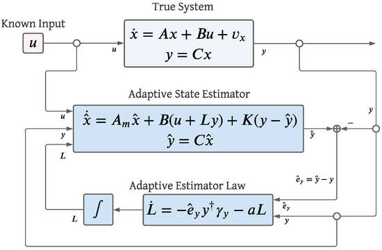
Figure 1. Control diagram for adaptive plant and state estimation accounting stochastic variations and environmental/health changes in the true system using known inputs and outputs.

2.1. Defining True System Dynamics

This case study assumes the true plant dynamics are linear time-invariant and either weak stochasticities or non-linearities $\left(v_x\right)$ are bounded and present in the dynamics:

$$\mathrm{T}\mathrm{r}\mathrm{u}\mathrm{e} \mathrm{S}\mathrm{y}\mathrm{s}\mathrm{t}\mathrm{e}\mathrm{m}\left\{\begin{array}{c}\dot{x}=Ax+Bu+v_x\hfill \\ y=Cx.\hfill \end{array}\right.$$

(2)

The input matrix $\left(B\right)$, output matrix $\left(C\right)$, output (external) state $\left(y\right)$, and input $\left(u\right)$ are assumed to be known and well understood. The true plant $\left(A\right)$ is assumed to have stable eigenvalues $\left(\mathrm{Re}\right(\sigma \left\{A\right\})<0)$, also referred to as a Hurwitz stable matrix. Given that the true plant experiences a health change, the true plant dynamics related to internal interactions and constitutive constants are unknown, but an initial plant model $\left(A_m\right)$ exists.

2.2. Overview of Updating the Reference Model

The following sections will derive a control law to minimize the state error between the true (Equation (2)) and model (Equation (3)) systems given the presence of stochasticities in the true system. Note that both the true and model systems match in dimensions but may differ in internal interactions and constitutive constants. The eigenvalues of the initial model plant $\left(A_m\right)$ are stable $(\mathrm{Re}\left(\sigma \left\{A_m\right\}\right)<0)$ and the weak stochasticities $\left(v_x\right)$ are unknown, bounded, and not accounted for in the reference model. Accounting for stochasticities in the true system adds an additional layer of complexity, potentially making the reference model dynamics less reliable.

$$\mathrm{Reference} \mathrm{Model}\left\{\begin{array}{c}{\dot{x}}_m=A_m{x}_m+Bu\hfill \\ y_m=C{x}_m\hfill \end{array}\right.$$

(3)

A board overview, the reference model considers both the input and output of the true system to modify its dynamics, aiming to minimize the estimated state errors $\{e_x,{\widehat{e}}_y\}$. To update the reference model, the true system’s plant is assumed to be decomposable into two components: the initial plant model $\left(A_m\right)$ and the plant correction term $\left(B{L}_{*}C\right)$:

$$A=A_m+B{L}_{*}C.$$

(4)

The decomposition of the true plant is structured so that the initial model can be updated and corrected in the estimator via a correction term $\left(L\right)$:

$$L\left(t\right)=∆L\left(t\right)+L_{*},$$

(5)

where $∆L$ is the variability-uncertainty term. Derived later, the correction term $\left(L\right)$ depends on the output state $\left(y\right)$ and the output error $\left({\widehat{e}}_y\right)$ between the model and true systems to adaptively update. By adjusting the reference dynamics, both internal and external errors can be guaranteed to converge to a neighborhood around zero asymptotically. Alternatively, for the derived control scheme to be feasible, the triplet of $(A,B,C)$ must be ASD $\ni A=A_m+B{L}_{*}C$ and $(A_m,B,C)$ is SPR.

2.3. Estimated State Error

Internal state $\left(x\right)$ information is often blended into a linear combination or omitted from the external state $\left(y\right)$. Therefore, an estimator is required to capture the full state vector $\left(x\right)$. However, the estimator complexity increases when the true system undergoes a health change and when bounded stochasticities exist in the system dynamics. Given the initial plant $\left(A_m\right)$ and using the true system’s external state, an estimator-observer can be created:

$$\mathrm{E}\mathrm{s}\mathrm{t}\mathrm{i}\mathrm{m}\mathrm{a}\mathrm{t}\mathrm{o}\mathrm{r}\left\{\begin{array}{c}\dot{\widehat{x}}=A_m\widehat{x}+B(u+Ly)\hfill \\ \widehat{y}=C\widehat{x}.\hfill \end{array}\right.$$

(6)

Note that the estimator and true systems are actuated using the same input $\left(u\right)$.

To minimize the error between both the estimator and the true systems, consider the following error states:

$$\begin{array}{c}{e}_x=\widehat{x}-x\\ {\widehat{e}}_y=C{e}_x.\end{array}$$

(7)

If both internal and external error states converge to zero ∋$\{e_x,{\widehat{e}}_y\}\underset{t\to \infty }{\to }0$, the true plant states have been numerically captured. To guarantee $\{e_x,{\widehat{e}}_y\}\underset{t\to \infty }{\to }0$, error state dynamics must be investigated:

$$\begin{array}{cc}\hfill {\dot{e}}_x=\dot{\widehat{x}}-\dot{x}& =\left(A_m\widehat{x}+B(u+Ly)\right)-(Ax+Bu+v_x)\hfill \\ \hfill & =A_m\widehat{x}+B(\underset{=L}{\underbrace{L_{*}+∆L}})y-\underset{=A}{\underbrace{\left(A_m+B{L}_{*}C\right)}}x-v_x\hfill \\ \hfill & =A_m{e}_x+B\underset{=w_x}{\underbrace{∆Ly}}+\underset{=-v_x}{\underbrace{v}}.\hfill \end{array}$$

(8)

Therefore, the state error equations can be written as follows:

$$\mathrm{Error} \mathrm{Equations}\left\{\begin{array}{c}{\dot{e}}_x=A_m{e}_x+B{w}_x+v\hfill \\ {\widehat{e}}_y=C{e}_x\hfill \end{array}\right.,$$

(9)

where $w_x=∆Ly$ and $v=-v_x$. In addition, the estimator can be modified to use fixed gain $\left(K\right)$:

$$\mathrm{Estimator} \mathrm{w}/\mathrm{Fixed} \mathrm{Gain}\left\{\begin{array}{c}\dot{\widehat{x}}=A_m\widehat{x}+B(u+Ly)+K(y-\widehat{y})\hfill \\ \widehat{y}=C\widehat{x}.\hfill \end{array}\right.$$

(10)

Resulting in the following error equations:

$$\mathrm{Error} \mathrm{Equations} w/\mathrm{Fixed} \mathrm{Gains}\left\{\begin{array}{c}{\dot{e}}_x=(A_m-KC)e_x+B{w}_x+v\hfill \\ {\widehat{e}}_y=C{e}_x.\hfill \end{array}\right.$$

(11)

In order to use the fixed gain $\left(K\right)$, $(A_m,C)$ must be observable and selected fixed gain $\left(K\right)$ must satisfy: $\mathrm{Re}\left(\sigma \left\{(A_m-KC)\right\}\right)<0$.

Independent of the desired estimator, $\{e_x,{\widehat{e}}_y\}$ cannot guarantee to converge to zero because of the two residual terms $\{B{w}_x,v\}$ in the error equations. An additional argument will be needed to remove and bound residual terms.

2.4. Lyapunov Stability for the Estimated State Error

Due to the presence of residual terms $\{B{w}_x,v\}$ in the error equations, $\{e_x,{\widehat{e}}_y\}\underset{t\to \infty }{\to }0$ cannot be guaranteed. To address this, Lyapunov stability analysis will be employed to minimize and possibly remove all of the error state. In this analysis, the internal error state $\left(e_x\right)$ will be minimized by considering an energy-like function for the error system with assumed real scalars:

$$V_e\left(e_x\right)={\displaystyle \frac{1}{2}}{e}_x^{†}{P}_x{e}_x;P_x>0,$$

(12)

where ${(·)}^{†}$ is the conjugate-transpose operator. Following, $P_x$ is a positive-definite $\left(\mathrm{Re}\left(\sigma \left\{P_x\right\}\right)>0\right)$ and self-adjoint matrix $(P_x=P_x^{†})$, alternatively written as $P_x>0$. To understand how the error state in the energy-like function evolves with time, take the time derivative of $V_e$ and substitute error dynamics:

$$\begin{array}{cc}\hfill 2{\dot{V}}_e& ={\dot{e}}_x^{†}{P}_x{e}_x+e_x^{†}{P}_x{\dot{e}}_x\hfill \\ \hfill & ={(A_m{e}_x+B{w}_x+v)}^{†}{P}_x{e}_x+e_x^{†}{P}_x(A_m{e}_x+B{w}_x+v)\hfill \\ \hfill & =e_x^{†}(A_m^{†}{P}_x+P_x{A}_m)e_x+2\underset{=e_x^{†}{P}_{x}B{w}_x}{\underbrace{{\left(B{w}_x\right)}^{†}{P}_x{e}_x}}+2\underset{=e_x^{†}{P}_{x}v}{\underbrace{v^{†}{P}_x{e}_x}}\hfill \\ \hfill & =e_x^{†}(A_m^{†}{P}_x+P_x{A}_m)e_x+2e_x^{†}{P}_{x}B{w}_x+2\underset{=(v,P_{x}e)}{\underbrace{v^{†}{P}_x{e}_x}}.\hfill \end{array}$$

(13)

The inner product operator is detonated as $(·,·)$.

Consider the SPR condition modified for the reference model:

$$\left\{\begin{array}{c}{A}_m^{†}{P}_x+P_x{A}_m<-Q_x\hfill \\ P_{x}B=C^{†},\hfill \end{array}\right.$$

(14)

where $Q_x>0$. Applying the reference model SPR condition on ${\dot{V}}_e$,

$$\begin{array}{cc}\hfill {\dot{V}}_e& =-{\displaystyle \frac{1}{2}}{e}_x^{†}{Q}_x{e}_x+\underset{={\widehat{e}}_y^{†}}{\underbrace{e_x^{†}{C}^{†}}}{w}_x+\underset{=(P_x{e}_x,v)}{\underbrace{(v,P_x{e}_x)}}\hfill \\ \hfill & =-{\displaystyle \frac{1}{2}}{e}_x^{†}{Q}_x{e}_x+\underset{=(w_x,{\widehat{e}}_y)}{\underbrace{({\widehat{e}}_y,w_x)}}+(P_x{e}_x,v).\hfill \end{array}$$

(15)

Removing the residual terms $\{({\widehat{e}}_y,w_x),(P_x{e}_x,v)\}$ in Equation (15), results in ${\dot{V}}_e\le 0$.

In order to remove or compensate the two residual terms in Equation (15), consider another Lyapunov energy-like function:

$$V_L(∆L)={\displaystyle \frac{1}{2}}\mathrm{tr}(∆L{\gamma }_y^{-1}∆L^{†});{\gamma }_y>0.$$

(16)

To determine the energy-like time rate of change of $V_L$, take the time derivative of $V_L$:

$$\begin{array}{c}\hfill {\dot{V}}_L=\underset{=\mathrm{tr}(∆L{\gamma }_y^{-1}∆{\dot{L}}^{†})}{\underbrace{\mathrm{tr}(∆\dot{L}{\gamma }_y^{-1}∆L^{†})}}.\end{array}$$

(17)

A control law is defined for the time rate of change of plant correction variance $(∆\dot{L})$:

$$∆\dot{L}=-{\widehat{e}}_y{y}^{†}{\gamma }_y-aL,$$

(18)

where a is a scalar. Additional constraints for a will be derived later. The term $aL$ in Equation (18) functions as a feedback filter. Substituting Equation (18) into Equation (17):

$$\begin{array}{cc}\hfill {\dot{V}}_L& =\mathrm{tr}(\underset{=∆\dot{L}}{\underbrace{(-{\widehat{e}}_y{y}^{†}{\gamma }_y-aL)}}{\gamma }_y^{-1}∆L^{†})=\mathrm{tr}(-{\widehat{e}}_y{y}^{†}{\gamma }_y{\gamma }_y^{-1}∆L^{†}-aL{\gamma }_y^{-1}∆L^{†})\hfill \\ \hfill & =-\mathrm{tr}({\widehat{e}}_y\underset{=w_x^{†}}{\underbrace{y^{†}∆L^{†}}})-\mathrm{tr}(aL{\gamma }_y^{-1}∆L^{†})=-\underset{=\mathrm{tr}\left(w_x^{†}{\widehat{e}}_y\right)}{\underbrace{\mathrm{tr}\left({\widehat{e}}_y{w}_x^{†}\right)}}-\mathrm{tr}(aL{\gamma }_y^{-1}∆L^{†})\hfill \\ \hfill & =-\underset{=(w_x,{\widehat{e}}_y)}{\underbrace{w_x^{†}{\widehat{e}}_y}}-\mathrm{tr}(aL{\gamma }_y^{-1}∆L^{†})=-\underset{=({\widehat{e}}_y,w_x)}{\underbrace{(w_x,{\widehat{e}}_y)}}-\mathrm{tr}(aL{\gamma }_y^{-1}∆L^{†}).\hfill \end{array}$$

(19)

Therefore, the closed-loop Lyapunov function for the error system can be written as follows:

$$V_{eL}(e_x,∆L)=V_e\left(e_x\right)+V_L(∆L)={\displaystyle \frac{1}{2}}{e}_x^{†}{P}_x{e}_x+{\displaystyle \frac{1}{2}}\mathrm{tr}(∆L{\gamma }_y^{-1}∆L^{†}).$$

(20)

Following, the closed-loop energy-like time rate of change for the error system follows:

$$\begin{array}{cc}\hfill {\dot{V}}_{eL}(e_x,∆L)& ={\dot{V}}_e\left(e_x\right)+{\dot{V}}_L(∆L)\hfill \\ \hfill & =-{\displaystyle \frac{1}{2}}{e}_x^{†}{Q}_x{e}_x+({\widehat{e}}_y,w_x)+(P_x{e}_x,v)-({\widehat{e}}_y,w_x)-\mathrm{tr}(aL{\gamma }_y^{-1}∆L^{†})\hfill \\ \hfill & =-{\displaystyle \frac{1}{2}}{e}_x^{†}{Q}_x{e}_x+(P_x{e}_x,v)-\mathrm{tr}(aL{\gamma }_y^{-1}∆L^{†}).\hfill \end{array}$$

(21)

While adaptive feedback has eliminated some of the residual terms in the closed-loop time derivative of the Lyapunov function, as demonstrated in Equation (21), residual terms still exist such that ${\dot{V}}_e\le 0$ is not guaranteed. As a result, the Barbalat–Lyapunov Lemma cannot be applied and therefore does not guarantee $e_x\underset{t\to \infty }{\to }0$ asymptotically. An additional argument will be presented to establish an upper bound on the estimated state error term, confining both the internal and external error to a neighborhood around zero.

2.5. Robustness Lyapunov Analysis for Error System

To determine the radius of convergence $\left(R_{*}\right)$ for the estimated state error $\left(e_x\right)$, each component from the right-hand side (RHS) of Equation (21) must be bounded. The following sections will derive bounds for each component on the RHS of Equation (21) by combining Sylvester’s Inequality, the Cauchy–Schwarz Inequality, and algebraic manipulation.

2.5.1. Upper Bounding $-{\displaystyle \frac{1}{2}}{e}_x^{†}{Q}_x{e}_x$

In order to find the upper bound of $-{\displaystyle \frac{1}{2}}{e}_x^{†}{Q}_x{e}_x$, first consider bounding the Lyapunov function in Equation (12) using Sylvester’s Inequality:

$${\displaystyle \frac{{\lambda }_{\min }\left(P_x\right)}{2}}\parallel e_x{\parallel }^2\le V_e={\displaystyle \frac{1}{2}}{e}_x^{†}{P}_x{e}_x\le {\displaystyle \frac{{\lambda }_{\max }\left(P_x\right)}{2}}{\parallel e_x\parallel }^2,$$

(22)

where $\{{\lambda }_{\min }\left(P_x\right),{\lambda }_{\max }\left(P_x\right)\}$ are the minimum and maximum eigenvalues of matrix $P_x$, respectively, and $\parallel e_x\parallel$ is the norm of the internal state error $\left(e_x\right)$. Continuing, $V_e$ can be upper-bounded via:

$$V_e\le {\displaystyle \frac{{\lambda }_{\max }\left(P_x\right)}{2}}{\parallel e_x\parallel }^2.$$

(23)

From Equation (23), $\parallel e_x{\parallel }^2$ can be solved for:

$${\displaystyle \frac{2V_e}{{\lambda }_{\max }\left(P_x\right)}}\le {\parallel e_x\parallel }^2.$$

(24)

Moving forward, consider using Sylvester’s inequality to bound the $-{\displaystyle \frac{1}{2}}{e}_x^{†}{Q}_x{e}_x$ term from Equation (21):

$$-{\displaystyle \frac{{\lambda }_{\min }\left(Q_x\right)}{2}}\parallel e_x{\parallel }^2\ge -{\displaystyle \frac{1}{2}}{e}_x^{†}{Q}_x{e}_x\ge -{\displaystyle \frac{{\lambda }_{\max }\left(Q_x\right)}{2}}{\parallel e_x\parallel }^2,$$

(25)

where $\{{\lambda }_{\min }\left(Q_x\right),{\lambda }_{\max }\left(Q_x\right)\}$ are the minimum and maximum eigenvalues of matrix $Q_x$, respectively. Therefore, the upper-bound of Equation (25) follows:

$$-{\displaystyle \frac{1}{2}}{e}_x^{†}{Q}_x{e}_x\le -{\displaystyle \frac{{\lambda }_{\min }\left(Q_x\right)}{2}}{\parallel e_x\parallel }^2.$$

(26)

Substituting the $\parallel e_x{\parallel }^2$ term from Equation (24) into Equation (26) results in the following:

$$\begin{array}{cc}\hfill -{\displaystyle \frac{1}{2}}{e}_x^{†}{Q}_x{e}_x& \le -{\displaystyle \frac{{\lambda }_{\min }\left(Q_x\right)}{2}}\underset{=\parallel e_x{\parallel }^2}{\underbrace{{\displaystyle \frac{2V_e}{{\lambda }_{\max }\left(P_x\right)}}}}\hfill \\ \hfill & \le -\underset{=2a>0}{\underbrace{{\displaystyle \frac{{\lambda }_{\min }\left(Q_x\right)}{{\lambda }_{\max }\left(P_x\right)}}}}{V}_e,\hfill \end{array}$$

(27)

where $a\ge {\displaystyle \frac{{\lambda }_{\min }\left(Q_x\right)}{2{\lambda }_{\max }\left(P_x\right)}}>0$ and is a scalar. Substituting Equation (27) into Equation (21),

$${\dot{V}}_{eL}\le -2a{V}_e+(P_x{e}_x,v)-a\mathrm{tr}(L{\gamma }_y^{-1}∆L^{†}),$$

(28)

results in an updated closed-loop energy-like time rate of change for the error system.

2.5.2. Upper Bounding $a\mathrm{tr}(L{\gamma }_y^{-1}∆L^{†})$

From Equation (28), let us focus on the $a\mathrm{tr}(L{\gamma }_y^{-1}∆L^{†})$ term. Recall: $L=∆L+L_{*}$, shown in Equation (5). Therefore, $a\mathrm{tr}(L{\gamma }_y^{-1}∆L^{†})$ can be alternatively expressed as follows:

$$\begin{array}{cc}\hfill a\mathrm{tr}(L{\gamma }_y^{-1}∆L^{†})& =a\mathrm{tr}((\underset{=L}{\underbrace{∆L+L_{*})}}{\gamma }_y^{-1}∆L^{†})\hfill \\ \hfill & =a\underset{=2V_L}{\underbrace{\mathrm{tr}(∆L{\gamma }_y^{-1}∆L^{†})}}+a\mathrm{tr}(L_{*}{\gamma }_y^{-1}∆L^{†})\hfill \\ \hfill & =2a{V}_L+a\mathrm{tr}(L_{*}{\gamma }_y^{-1}∆L^{†}).\hfill \end{array}$$

(29)

Substituting Equation (29) into Equation (28):

$$\begin{array}{cc}\hfill {\dot{V}}_{eL}& \le -2a{V}_e+(P_x{e}_x,v)-2a{V}_L-a\mathrm{tr}(L_{*}{\gamma }_y^{-1}∆L^{†})\hfill \\ \hfill & \le -2a(\underset{=V_{eL}}{\underbrace{V_e+V_L}})+(P_x{e}_x,v)-a\mathrm{tr}(L_{*}{\gamma }_y^{-1}∆L^{†}).\hfill \end{array}$$

(30)

Alternatively, Equation (30) can be written as follows:

$$\begin{array}{cc}\hfill {\dot{V}}_{eL}+2a{V}_{eL}& \le (P_x{e}_x,v)-a\mathrm{tr}(L_{*}{\gamma }_y^{-1}∆L^{†}).\hfill \end{array}$$

(31)

2.5.3. Upper Bounding $(P_x{e}_x,v)$

The right-hand side of Equation (31) can be upper bounded by taking the absolute value of terms:

$$\begin{array}{cc}\hfill {\dot{V}}_{eL}+2a{V}_{eL}& \le |(P_x{e}_x,v)|+a|\mathrm{tr}(L_{*}{\gamma }_y^{-1}∆L^{†})|.\hfill \end{array}$$

(32)

To further bound $\left\{\right|(P_x{e}_x,v)|,a|\mathrm{tr}(L_{*}{\gamma }_y^{-1}∆L^{†})\left|\right\}$, recall the Cauchy–Schwarz inequality: $\left|(u,v)\right|\le {(u,u)}^{{\displaystyle \frac{1}{2}}}{(v,v)}^{{\displaystyle \frac{1}{2}}}$. Therefore, applying the Cauchy–Schwarz’s Inequality on $\left|\right(P_x{e}_x,v\left)\right|$:

$$\begin{array}{cc}\hfill |(P_x{e}_x,v)|=|e_x^{†}{P}_{x}v|=|e_x^{†}{P}_x^{{\displaystyle \frac{1}{2}}}{P}_x^{{\displaystyle \frac{1}{2}}}v|=|(P_x^{{\displaystyle \frac{1}{2}}}{e}_x,P_x^{{\displaystyle \frac{1}{2}}}v)|& \le {(P_x^{{\displaystyle \frac{1}{2}}}{e}_x,P_x^{{\displaystyle \frac{1}{2}}}{e}_x)}^{{\displaystyle \frac{1}{2}}}{(P_x^{{\displaystyle \frac{1}{2}}}v,P_x^{{\displaystyle \frac{1}{2}}}v)}^{{\displaystyle \frac{1}{2}}}\hfill \\ \hfill & \le \underset{={\left(2V_e\right)}^{{\displaystyle \frac{1}{2}}}\le {\left(2V_{eL}\right)}^{{\displaystyle \frac{1}{2}}}}{\underbrace{{(P_x{e}_x,e_x)}^{{\displaystyle \frac{1}{2}}}}}{(P_{x}v,v)}^{{\displaystyle \frac{1}{2}}}\hfill \\ \hfill & \le {\left(2V_{eL}\right)}^{{\displaystyle \frac{1}{2}}}{(P_{x}v,v)}^{{\displaystyle \frac{1}{2}}}.\hfill \end{array}$$

(33)

From Equation (33), the ${(P_{x}v,v)}^{{\displaystyle \frac{1}{2}}}$ term can be further bounded by applying Sylvester’s Inequality:

$$\begin{array}{c}\hfill {\lambda }_{\min }{\left(P_x\right)}^{{\displaystyle \frac{1}{2}}}\parallel v\parallel \le {(P_{x}v,v)}^{{\displaystyle \frac{1}{2}}}\le {\lambda }_{\max }{\left(P_x\right)}^{{\displaystyle \frac{1}{2}}}\parallel v\parallel .\end{array}$$

(34)

Therefore, the upper-bound of ${(P_{x}v,v)}^{{\displaystyle \frac{1}{2}}}$ follows:

$${(P_{x}v,v)}^{{\displaystyle \frac{1}{2}}}\le {\lambda }_{\max }{\left(P_x\right)}^{{\displaystyle \frac{1}{2}}}\parallel v\parallel .$$

(35)

Given that norm of the bounded-stochastic waveform $(\parallel v\parallel )$ can vary with time, the upper bound of $\parallel v\parallel$ can be expressed as a supremum ($sup$) such that

$$M_v>0\ni \underset{t\ge 0}{sup}\parallel v\left(t\right)\parallel \le M_v.$$

(36)

Using the result from Equation (36), the upper-bound of ${(P_{x}v,v)}^{{\displaystyle \frac{1}{2}}}$ from Equation (35) can be expressed as follows:

$${(P_{x}v,v)}^{{\displaystyle \frac{1}{2}}}\le {\lambda }_{\max }{\left(P_x\right)}^{{\displaystyle \frac{1}{2}}}{M}_v.$$

(37)

Therefore, using the results from Equations (33) and (37), the upper-bound of $\left|\right(P_x{e}_x,v\left)\right|$ can be expressed as follows:

$$|(P_x{e}_x,v)|\le {\left(2V_{eL}\right)}^{{\displaystyle \frac{1}{2}}}{(P_{x}v,v)}^{{\displaystyle \frac{1}{2}}}\le {\left(2V_{eL}\right)}^{{\displaystyle \frac{1}{2}}}{\lambda }_{\max }{\left(P_x\right)}^{{\displaystyle \frac{1}{2}}}{M}_v.$$

(38)

2.5.4. Upper Bounding $\left|\mathrm{tr}\right(L_{*}{\gamma }_y^{-1}∆L^{†}\left)\right|$

Transitioning, lets consider bounding the $\left|\mathrm{tr}\right(L_{*}{\gamma }_y^{-1}∆L^{†}\left)\right|$ term from Equation (32). Using the Cauchy–Schwarz inequality, alternatively written as $|\mathrm{tr}\left(A{B}^{†}\right)|\le \mathrm{tr}{\left(A{A}^{†}\right)}^{{\displaystyle \frac{1}{2}}}\mathrm{tr}{\left(B{B}^{†}\right)}^{{\displaystyle \frac{1}{2}}}$, on $\left|\mathrm{tr}\right(L_{*}{\gamma }_y^{-1}∆L^{†}\left)\right|$:

$$\begin{array}{cc}\hfill \left|\mathrm{tr}\right(L_{*}{\gamma }_y^{-1}∆L^{†}\left)\right|& \le \mathrm{tr}{\left(L_{*}{\gamma }_y^{-1}{L}_{*}^{†}\right)}^{{\displaystyle \frac{1}{2}}}\underset{={\left(2V_L\right)}^{{\displaystyle \frac{1}{2}}}\le {\left(2V_{eL}\right)}^{{\displaystyle \frac{1}{2}}}}{\underbrace{\mathrm{tr}{(∆L{\gamma }_y^{-1}∆L^{†})}^{{\displaystyle \frac{1}{2}}}}}\hfill \\ \hfill & \le \mathrm{tr}{\left(L_{*}{\gamma }_y^{-1}{L}_{*}^{†}\right)}^{{\displaystyle \frac{1}{2}}}{\left(2V_{eL}\right)}^{{\displaystyle \frac{1}{2}}}.\hfill \end{array}$$

(39)

Using the trace operator $\left(\mathrm{tr}\right)$ property of invariant under circular shifts (i.e., $\mathrm{tr}\left(ABC\right)=\mathrm{tr}\left(CAB\right)=\mathrm{tr}\left(BCA\right)$), the $\mathrm{tr}{\left(L_{*}{\gamma }_y^{-1}{L}_{*}^{†}\right)}^{{\displaystyle \frac{1}{2}}}$ term from Equation (39) can be rewritten as follows:

$$\begin{array}{c}\hfill \mathrm{tr}{\left(L_{*}{\gamma }_y^{-1}{L}_{*}^{†}\right)}^{{\displaystyle \frac{1}{2}}}=\mathrm{tr}{\left(L_{*}^{†}{L}_{*}{\gamma }_y^{-1}\right)}^{{\displaystyle \frac{1}{2}}}.\end{array}$$

(40)

Equation (40) can be upper bounded by applying the Cauchy–Schwarz inequality:

$$\begin{array}{cc}\hfill \mathrm{tr}{\left(L_{*}^{†}{L}_{*}{\gamma }_y^{-1}\right)}^{{\displaystyle \frac{1}{2}}}\le |\mathrm{tr}{\left(L_{*}^{†}{L}_{*}{\gamma }_y^{-1}\right)}^{{\displaystyle \frac{1}{2}}}|& \le \mathrm{tr}{\left(L_{*}^{†}{L}_{*}{L}_{*}^{†}{L}_{*}\right)}^{{\displaystyle \frac{1}{4}}}\mathrm{tr}{\left({\gamma }_y^{-1}{\gamma }_y^{-1}\right)}^{{\displaystyle \frac{1}{4}}}\hfill \\ \hfill & \le \mathrm{tr}{\left(L_{*}^{†}{L}_{*}\right)}^{{\displaystyle \frac{1}{2}}}\mathrm{tr}{\left({\gamma }_y^{-1}\right)}^{{\displaystyle \frac{1}{2}}}.\hfill \end{array}$$

(41)

For notation purposes, allow the following assumptions:

$$M_k>0\ni \mathrm{tr}{\left(L_{*}^{†}{L}_{*}\right)}^{{\displaystyle \frac{1}{2}}}\le M_k$$

(42)

and

$$\mathrm{tr}\left({\gamma }_y^{-1}\right)\le {\left({\displaystyle \frac{M_v}{a{M}_k}}\right)}^2.$$

(43)

Substituting Equations (42) and (43) in Equation (41),

$$\begin{array}{cc}\hfill \mathrm{tr}{\left(L_{*}^{†}{L}_{*}{\gamma }_y^{-1}\right)}^{{\displaystyle \frac{1}{2}}}& \le \mathrm{tr}{\left(L_{*}^{†}{L}_{*}\right)}^{{\displaystyle \frac{1}{2}}}\mathrm{tr}{\left({\gamma }_y^{-1}\right)}^{{\displaystyle \frac{1}{2}}}\hfill \\ \hfill & \le M_k\left({\displaystyle \frac{M_v}{a{M}_k}}\right)\hfill \\ \hfill & \le \left({\displaystyle \frac{M_v}{a}}\right).\hfill \end{array}$$

(44)

Following, Equation (44) can be substituted in Equation (39):

$$|\mathrm{tr}(L_{*}{\gamma }_y^{-1}∆L^{†})|\le \mathrm{tr}{\left(L_{*}{\gamma }_y^{-1}{L}_{*}^{†}\right)}^{{\displaystyle \frac{1}{2}}}{\left(2V_{eL}\right)}^{{\displaystyle \frac{1}{2}}}\le \left({\displaystyle \frac{M_v}{a}}\right){\left(2V_{eL}\right)}^{{\displaystyle \frac{1}{2}}}.$$

(45)

2.5.5. Combining Bounds to Determine Radius of Convergence $\left(R_{*}\right)$

Using the result from Equations (38) and (45) in Equation (32) results in the following:

$$\begin{array}{cc}\hfill {\dot{V}}_{eL}+2a{V}_{eL}& \le |(P_x{e}_x,v)|+a|\mathrm{tr}(L_{*}{\gamma }_y^{-1}∆L^{†})|\hfill \\ \hfill & \le {\lambda }_{\max }{\left(P_x\right)}^{{\displaystyle \frac{1}{2}}}{M}_v{\left(2V_{eL}\right)}^{{\displaystyle \frac{1}{2}}}+a\left({\displaystyle \frac{M_v}{a}}\right){\left(2V_{eL}\right)}^{{\displaystyle \frac{1}{2}}}\hfill \\ \hfill & \le ({\lambda }_{\max }{\left(P_x\right)}^{{\displaystyle \frac{1}{2}}}+1)M_v{\left(2V_{eL}\right)}^{{\displaystyle \frac{1}{2}}}.\hfill \end{array}$$

(46)

Following, Equation (46) can also be expressed as follows:

$$\begin{array}{cc}\hfill {\displaystyle \frac{{\dot{V}}_{eL}+2a{V}_{eL}}{V_{eL}^{\frac{1}{2}}}}& \le \sqrt{2}({\lambda }_{\max }{\left(P_x\right)}^{{\displaystyle \frac{1}{2}}}+1)M_v.\hfill \end{array}$$

(47)

Consider an alternative expression for the left-hand side of Equation (47):

$$\begin{array}{cc}\hfill {\displaystyle \frac{d}{dt}}(2e^{at}{V}_{eL}^{{\displaystyle \frac{1}{2}}})& =e^{at}{V}_{eL}^{-{\displaystyle \frac{1}{2}}}{\dot{V}}_{eL}+2a{e}^{at}{V}_e^{{\displaystyle \frac{1}{2}}}\hfill \\ \hfill & ={\displaystyle \frac{{\dot{V}}_{eL}+2a{V}_{eL}}{V_{eL}^{\frac{1}{2}}}}{e}^{at}.\hfill \end{array}$$

(48)

Therefore, Equation (47) can be expressed as follows:

$$\begin{array}{cc}\hfill {\displaystyle \frac{d}{dt}}(2e^{at}{V}_{eL}^{{\displaystyle \frac{1}{2}}})& \le \sqrt{2}({\lambda }_{\max }{\left(P_x\right)}^{{\displaystyle \frac{1}{2}}}+1)M_v{e}^{at}.\hfill \end{array}$$

(49)

Integrating and evaluating both sides of Equation (49) from 0 to $\tau$ results in the following:

$$\begin{array}{cc}\hfill (2e^{a\tau }{V}_{eL}{\left(\tau \right)}^{{\displaystyle \frac{1}{2}}}-2V_{eL}{\left(0\right)}^{{\displaystyle \frac{1}{2}}})& \le {\displaystyle \frac{\sqrt{2}({\lambda }_{\max }{\left(P_x\right)}^{\frac{1}{2}}+1)M_v}{a}}(e^{a\tau }-1).\hfill \end{array}$$

(50)

Solving for $V_{eL}{\left(\tau \right)}^{{\displaystyle \frac{1}{2}}}$:

$$V_{eL}{\left(\tau \right)}^{{\displaystyle \frac{1}{2}}}\le e^{-a\tau }{V}_{eL}{\left(0\right)}^{{\displaystyle \frac{1}{2}}}+{\displaystyle \frac{\sqrt{2}({\lambda }_{\max }{\left(P_x\right)}^{\frac{1}{2}}+1)M_v}{2a}}(1-e^{-a\tau }).$$

(51)

From Equation (51), $V_{eL}^{{\displaystyle \frac{1}{2}}}$ can be expressed as being bounded for all $\tau \ge 0$, which indicates that $V_{eL}$ is also bounded. Given $V_{eL}$ is a function of $\{e_x,∆L\}$, it follows that both $\{e_x,∆L\}$ are likewise bounded.

Continuing, $V_{eL}{\left(\tau \right)}^{{\displaystyle \frac{1}{2}}}$ can be lower bounded by considering the following:

$${\displaystyle \frac{1}{\sqrt{2}}}{\lambda }_{\min }{\left(P_x\right)}^{{\displaystyle \frac{1}{2}}}\parallel e_x\parallel \le V_e{\left(\tau \right)}^{{\displaystyle \frac{1}{2}}}\le V_e{\left(\tau \right)}^{{\displaystyle \frac{1}{2}}}+V_L{\left(\tau \right)}^{{\displaystyle \frac{1}{2}}}\le V_{eL}{\left(\tau \right)}^{{\displaystyle \frac{1}{2}}}.$$

(52)

Substituting the lower bound for Equation (52) lower bound into Equation (51),

$${\displaystyle \frac{1}{\sqrt{2}}}{\lambda }_{\min }{\left(P_x\right)}^{{\displaystyle \frac{1}{2}}}\parallel e_x\parallel \le e^{-a\tau }{V}_{eL}{\left(0\right)}^{{\displaystyle \frac{1}{2}}}+{\displaystyle \frac{\sqrt{2}({\lambda }_{\max }{\left(P_x\right)}^{\frac{1}{2}}+1)M_v}{2a}}(1-e^{-a\tau }).$$

(53)

Solving for $\parallel e_x\parallel$ results in the following:

$$\parallel e_x\parallel \le {\displaystyle \frac{\sqrt{2}{V}_{eL}{\left(0\right)}^{\frac{1}{2}}}{{\lambda }_{\min }{\left(P_x\right)}^{\frac{1}{2}}}}{e}^{-a\tau }+{\displaystyle \frac{({\lambda }_{\max }{\left(P_x\right)}^{\frac{1}{2}}+1)M_v}{{\lambda }_{\min }{\left(P_x\right)}^{\frac{1}{2}}a}}(1-e^{-a\tau }).$$

(54)

Taking the supremum of $\parallel e_x\parallel$ as time approaches infinity results in the following:

$$\underset{t\to \infty }{\lim \sup }\parallel e_x\parallel \le {\displaystyle \frac{1+\sqrt{{\lambda }_{\max }\left(P_x\right)}}{a\sqrt{{\lambda }_{\min }\left(P_x\right)}}}{M}_v\equiv R_{*}.$$

(55)

Therefore, upper bounding the error state norm to a radius of convergence $\left(R_{*}\right)$ around a neighborhood of zero.

Alternatively, if the following adaptive law is considered,

$$∆\dot{L}=-{\widehat{e}}_y{y}^{†}{\gamma }_y,$$

(56)

where $aL=0$ from Equation (18), robustness proof can be modified accordingly, resulting in the following radius of convergence:

$$\underset{t\to \infty }{\lim \sup }\parallel e_x\parallel \le {\displaystyle \frac{\sqrt{{\lambda }_{\max }\left(P_x\right)}}{a\sqrt{{\lambda }_{\min }\left(P_x\right)}}}{M}_v\equiv R_{*}.$$

(57)

This version of the robustness proof has looser constraints, as Equation (43) need not be satisfied. Regardless of the adaptive law selected, robustness proof can be extended without loss of generality to consider the error system with fixed gains, as in Equation (11).

2.5.6. Determining the Bounds for $∆L$

In order to determine a radius of convergence for $∆L$, recall $V_L={\displaystyle \frac{1}{2}}\mathrm{tr}(∆L{\gamma }_y^{-1}∆L^{†})$ from Equation (16). Using the cyclic property of the trace, $V_L$ can be alternatively expressed as follows:

$$V_L={\displaystyle \frac{1}{2}}\mathrm{tr}(∆L^{†}∆L{\gamma }_y^{-1}).$$

(58)

Applying the Cauchy–Schwarz inequality on Equation (58),

$$\begin{array}{cc}\hfill {\displaystyle \frac{1}{2}}\mathrm{tr}(∆L^{†}∆L{\gamma }_y^{-1})& \le {\displaystyle \frac{1}{2}}\mathrm{tr}{(∆L^{†}∆L∆L^{†}∆L)}^{{\displaystyle \frac{1}{2}}}\mathrm{tr}{\left({\gamma }_y^{-1}{\gamma }_y^{-1}\right)}^{{\displaystyle \frac{1}{2}}}\hfill \\ \hfill & \le {\displaystyle \frac{1}{2}}\underset{={\parallel ∆L\parallel }_F^2}{\underbrace{\mathrm{tr}(∆L^{†}∆L)}}\mathrm{tr}\left({\gamma }_y^{-1}\right),\hfill \end{array}$$

(59)

where ${\parallel ∆L\parallel }_F$ is the Frobenius norm of $∆L$. Given that ${\parallel ∆L\parallel }_F$ can be lower-bounded by additional norms, the norm of $∆L$ must be constricted to ${\parallel ∆L\parallel }_F$. Using the previous assumption from Equation (43) on Equation (59) results in the following:

$$V_L\le {\displaystyle \frac{1}{2}}{\parallel ∆L\parallel }_F^2\underset{=\mathrm{tr}\left({\gamma }_y^{-1}\right)}{\underbrace{{\left({\displaystyle \frac{M_v}{a{M}_k}}\right)}^2}}.$$

(60)

Therefore, $V_L^{{\displaystyle \frac{1}{2}}}$ can be expressed as follows:

$$V_L^{{\displaystyle \frac{1}{2}}}\le {\displaystyle \frac{1}{\sqrt{2}}}{\parallel ∆L\parallel }_F\left({\displaystyle \frac{M_v}{a{M}_k}}\right).$$

(61)

Meaning, Equation (51) can alternatively be lower bounded by $V_L^{{\displaystyle \frac{1}{2}}}:$

$$V_L^{{\displaystyle \frac{1}{2}}}\le {\displaystyle \frac{1}{\sqrt{2}}}{\parallel ∆L\parallel }_F\left({\displaystyle \frac{M_v}{a{M}_k}}\right)\le V_{eL}{\left(\tau \right)}^{{\displaystyle \frac{1}{2}}}\le e^{-a\tau }{V}_{eL}{\left(0\right)}^{{\displaystyle \frac{1}{2}}}+{\displaystyle \frac{\sqrt{2}({\lambda }_{\max }{\left(P_x\right)}^{\frac{1}{2}}+1)M_v}{2a}}(1-e^{-a\tau }).$$

(62)

Solving for ${\parallel ∆L\parallel }_F$ in Equation (62):

$${\parallel ∆L\parallel }_F\le \left({\displaystyle \frac{\sqrt{2}a{M}_k}{M_v}}\right)e^{-a\tau }{V}_{eL}{\left(0\right)}^{{\displaystyle \frac{1}{2}}}+({\lambda }_{\max }{\left(P_x\right)}^{{\displaystyle \frac{1}{2}}}+1)M_k(1-e^{-a\tau }).$$

(63)

Taking the supremum of ${\parallel ∆L\parallel }_F$ as time approaches infinity results in the following:

$$\underset{t\to \infty }{\lim \sup }{\parallel ∆L\parallel }_F\le \left(\sqrt{{\lambda }_{\max }\left(P_x\right)}+1\right)M_k\equiv R_{**}.$$

(64)

Therefore, upper-bounding the correction variance norm to a radius of convergence of $R_{**}$. Alternatively, if the control law in Equation (56) is considered, the supremum of $\parallel ∆L\parallel$ as time approaches infinity results in the following:

$$\underset{t\to \infty }{\lim \sup }{\parallel ∆L\parallel }_F\le \sqrt{{\lambda }_{\max }\left(P_x\right)}{M}_k\equiv R_{**}.$$

(65)

2.5.7. Alternative $∆L$ Bound

As detailed in the previous section, the bound on $∆L$ depends on the assumption outlined in Equation (43). Consider the case where the adaptive law is considered without the feedback filter $(aL=0)$, as detailed in Equation (56), and the Equation (43) constraint is removed. Applying Sylvester’s Inequality to ${\gamma }_y^{-1}$

$${\lambda }_{\min }\left({\gamma }_y^{-1}\right)\le {\gamma }_y^{-1}\le {\lambda }_{\max }\left({\gamma }_y^{-1}\right),$$

(66)

Therefore, $V_L$ can be alternatively bounded:

$${\displaystyle \frac{{\lambda }_{\min }\left({\gamma }_y^{-1}\right)}{2}}{\parallel ∆L\parallel }_F^2\le V_L={\displaystyle \frac{1}{2}}\mathrm{tr}(∆L{\gamma }_y^{-1}∆L^{†})\le {\displaystyle \frac{{\lambda }_{\max }\left({\gamma }_y^{-1}\right)}{2}}{\parallel ∆L\parallel }_F^2.$$

(67)

Meaning, the lower bound of $V_L^{{\displaystyle \frac{1}{2}}}$ can be expressed as follows:

$${\displaystyle \frac{\sqrt{{\lambda }_{\min }\left({\gamma }_y^{-1}\right)}}{\sqrt{2}}}{\parallel ∆L\parallel }_F\le V_L^{{\displaystyle \frac{1}{2}}}.$$

(68)

Using the result from Equation (68) to lower bound Equation (51):

$${\displaystyle \frac{\sqrt{{\lambda }_{\min }\left({\gamma }_y^{-1}\right)}}{\sqrt{2}}}{\parallel ∆L\parallel }_F\le V_L^{{\displaystyle \frac{1}{2}}}\le V_{eL}{\left(\tau \right)}^{{\displaystyle \frac{1}{2}}}\le e^{-a\tau }{V}_{eL}{\left(0\right)}^{{\displaystyle \frac{1}{2}}}+{\displaystyle \frac{\sqrt{2}({\lambda }_{\max }{\left(P_x\right)}^{\frac{1}{2}}+1)M_v}{2a}}(1-e^{-a\tau }).$$

(69)

Solving and taking the supremum of $\parallel ∆L\parallel$ from Equation (69) as time approaches infinity results in the following:

$$\underset{t\to \infty }{\lim \sup }{\parallel ∆L\parallel }_F={\displaystyle \frac{\sqrt{{\lambda }_{\max }\left(P_x\right)}{M}_v}{\sqrt{{\lambda }_{\min }\left({\gamma }_y^{-1}\right)}a}}\equiv R_{**}.$$

(70)

There are several bounds for $\parallel L\parallel$ as depicted in Equations (64), (65), and (70); however, they are all dependent on the assumptions and constraints of the control problem.

2.6. Main Result Summarized

In conclusion, given that the true system experiences a health change and there exist weak and bounded stochasticities $\left(v_x\right)$ in the true system, robustness proof with adaptive law (Equation (71)) guarantees internal state error to converge to a radius $\left(R_{*}\right)$ around the neighborhood of zero, $e_x\underset{t\to \infty }{\to }{R}_{*}$. However, stability proof is only valid when the triples of the model $(A_m,B.C)$ and true system $(A,B,C)$ are SPR and ASD, respectively, such that the true plant can be written as $A\equiv A_m+B{L}_{*}C$. Proof does guarantee the plant variance $(∆L)$ to be bounded; however, there is no guarantee of $∆L\underset{t\to \infty }{\to }0$. If $∆L\underset{t\to \infty }{\to }0$ numerically, the true system’s dynamics or some energy equivalence has been numerically captured. The control diagram for proof is shown in Figure 1.

$$\mathrm{Adaptive} \mathrm{Estimation} \mathrm{Law}\left\{\begin{array}{c}\dot{L}=∆\dot{L}=-{\widehat{e}}_y{y}^{†}{\gamma }_y-aL\hfill \end{array}\right.$$

(71)

3. Illustrative Example

This section will demonstrate an illustrative example implementing the control diagram, Figure 1, for state estimation given the uncertainty in the model plant and stochasticities $\left(v_x\right)$ existing in the true dynamics. True and model values for this example are modified from [17]. All initial values for $\{x\left(0\right),\widehat{x}\left(0\right),L\left(0\right)\}$ are equal to zero, while the values for $v_x$ range between $\pm 0.25$. While the illustrative example may be perceived as limited, the full capacity of the theorem can be constrained by the specific application and the local uncertainties related to certain operational points. View Appendix A for an alternative example, where the true plant is altered and the fixed gain in the estimator is not considered. Note the assumptions and constraints for this control scheme detailed in Theorem 1.

3.1. State Space Representations for Reference and True Systems

In order to implement the proposed control scheme, an initial model plant $\left(A_m\right)$ must exist. Allow the model system, as defined in Equation (3), to have the following properties:

$$A_m=\left[\begin{array}{ccc}-7& 2& 4\\ -2& -1& 2\\ -2& 2& -1\end{array}\right];B=\left[\begin{array}{cc}0& 1\\ .7& 0\\ 2& 0\end{array}\right];C=\left[\begin{array}{ccc}0.5& 0& 1\\ 1.2& 0& .25\end{array}\right];x\left(0\right)=0.$$

(72)

For the control approach to be viable, as defined in Theorem 1, allow $A\in sp\{A_m,B{L}_{*}C\}\ni A=A_m+B{L}_{*}C$. For this example, allow the fixed correction matrix $\left(L_{*}\right)$ to follow:

$$L_{*}=\left[\begin{array}{cc}{L}_{11}& L_{12}\\ L_{21}& L_{22}\end{array}\right]=\left[\begin{array}{cc}-3& 4\\ -1& -5\end{array}\right].$$

(73)

Therefore, the true system, as defined in Equation (2), is written as follows:

$$A=A_m+B{L}_{*}C=\left[\begin{array}{ccc}-13& 2& 1.75\\ 0.31& -1& 0.6\\ 4.6& 2& -5\end{array}\right];B=\left[\begin{array}{cc}0& 1\\ .7& 0\\ 2& 0\end{array}\right];C=\left[\begin{array}{ccc}0.5& 0& 1\\ 1.2& 0& .25\end{array}\right];x\left(0\right)=0.$$

(74)

Allow the stochasticities to be bounded such supremum of $\parallel v_x\parallel =0.25$. Recall that internal interactions and constitutive constants of the true system’s plant $\left(A\right)$ are unknown, but an initial model exists $\left(A_m\right)$ such that plant dimensions correspond. Following the input and output matrices $\{B,C\}$ are known.

Giving both model and true systems, defined by proprieties in Equations (72) and (74), respectively, a unit step input, results in discrepancies in steady-state output responses, shown in Figure 2. The variation in the output response becomes particularly evident when comparing the eigenvalues of the model and the true plant:

$$\begin{array}{c}\sigma \left\{A_m\right\}=\{-1,-3,-5\}\\ \sigma \left\{A\right\}\approx \{-0.5,-4.6,-14.4\}.\end{array}$$

(75)

3.2. Defining the Known Input $\left(u\right)$

The estimator and true systems are actuated using the same known bounded and continuous input $\left(u\right)$. For this example, allow the known input to be defined as follows:

$$u=\left[\begin{array}{c}-3+1.2sin\left(t\right)\\ 2+cos\left(4t\right)\end{array}\right].$$

(76)

This input may represent a known disturbance or any arbitrary excitation used to query the system. Alternatively, the selected input can correspond to the control input that regulates the true system response. Crucially, both the true system and the estimator must be subjected to the same input, beyond the stochastic variation acting solely on the true system.

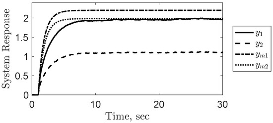
Figure 2. True $\left(y\right)$ and reference $\left(y_m\right)$ system’s output response given a unit-step input $\left(u\right)$.

3.3. Adaptive State Estimation

The following section implements the control scheme outlined in Theorem 1 and illustrated in Figure 1. The proof demonstrates that the proposed control scheme can be executed with or without a fixed gain $\left(K\right)$ in the estimator. Utilizing a fixed gain can offer certain advantages, as it can influence the convergence of the state error. Both cases presented will utilize the same fixed gain, which is derived using a Linear Quadratic Regulator with $Q=I_3$ and $R=1$. In contrast, the adaptive laws will exhibit slight variations, as noted in Equations (56) and (71). Furthermore, the interaction tuning term $\left({\gamma }_y\right)$ controls the estimator’s sensitivity to output error, directly impacting how the error state converges. There are numerical limits for ${\gamma }_y$, if increased excessively, the estimator can diverge. For this example, ${\gamma }_y=I_2$.

3.3.1. Adaptive Control Scheme Without a Feedback  Filter ($aL=0$)

The control scheme illustrated in Figure 1 is implemented with a fixed gain $\left(K\right)$ and the adaptive law outlined in Equation (56), where ${\gamma }_y=I$ and $aL=0$. As illustrated in Figure 3 and Figure 4, both internal and external state errors converge to a radius around zero. Although the proof establishes that the internal and external error states will converge to a neighborhood around zero, it only assures that the variance matrix $(∆L)$ will remain bounded. In this particular example, numerical results indicate as $∆L$ collapses such that $L\underset{t\to \infty }{\to }{L}_{*}$, shown in Figure 5. Consequently, as $L\underset{t\to \infty }{\to }{L}_{*}$, the internal error radius further reduces to a smaller neighborhood around zero, as seen in Figure 3b.

Due to the stochastic variations in the true system, values of L will show variability as time approaches infinity. In order to compare the estimated plant with the true system, the last 20 s of L’s simulated data were averaged, denoted by $L_{avg}$. Consequently, the $L_{avg}$ for this example is as follows:

$$L_{avg}\approx \left[\begin{array}{cc}-3& 4\\ -1.02& -4.95\end{array}\right].$$

(77)

Therefore, the estimated plant $\left(A_{est}\right)$ can be expressed as follows:

$$A_{est}\approx A_m+B{L}_{avg}C\approx \left[\begin{array}{ccc}-13.46& 2& 1.74\\ 0.32& -1& 0.60\\ 4.62& 2& -5\end{array}\right],$$

(78)

where the eigenvalues of $A_{est}$ are $\sigma \left\{A_{est}\right\}\approx \{-0.51,-4.64,-14.32\}$. Observe the similarities in internal interactions and constitutive constants between true and estimated plants, as shown in Equation (74) and Equation (78), respectively.

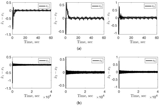
Figure 3. Both sub-figures (a,b) illustrate the internal state error $\left(e_x\right)$ converging to a radius $\left(R_{*}\right)$ around a neighborhood of zero; however, they do so at two different time histories. The implemented control scheme used a fixed gain and $aL=0$.

Figure 4. External state error $\left({\widehat{e}}_y\right)$ converging to a radius around zero with the use of the fixed gain and $aL=0$.

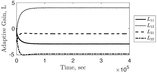
Figure 5. Adaptive Gain $L\left(t\right)$ converging to $L_{*}$ with the use of the fixed gain $(K\ne 0)$ and $aL=0$.

3.3.2. Adaptive Control Scheme with a Feedback Filter ($aL\ne 0$)

In this section, the control scheme illustrated in Figure 1 and adaptive law (Equation (71)) are implemented using a fixed gain (i.e., $K\ne 0$), ${\gamma }_y=I$, and $a=0.05$. As shown in Figure 6 and Figure 7, both internal and external state errors converge to a radius around zero. Although there is variability in L as time approaches infinity, Figure 8, the average L term $\left(L_{avg}\right)$ as time approaches infinity follows:

$$L_{avg}\approx \left[\begin{array}{cc}-0.78& -0.38\\ -2.77& -1.4\end{array}\right].$$

(79)

Consequently, this leads to the following estimated true plant matrix $\left(A_{est}\right)$:

$$A_{est}\approx A_m+B{L}_{avg}C\approx \left[\begin{array}{ccc}-10.08& 2& 0.88\\ -2.59& -1& 1.39\\ -3.70& 2& -2.75\end{array}\right],$$

(80)

where the eigenvalues are given by $\sigma \left\{A_{est}\right\}\approx \{-0.94,-3.72,-9.17\}$. Although the estimated plant matrix does not equal the true plant, $A_{est}$ gives a better intuition into the true plant $\left(A\right)$ compared to the initial model plant $\left(A_m\right)$ and grants ${sup}_{t\ge 0}\parallel e_x\parallel =R_{*}$. For this example, it is important to note that as $t\to \infty$, there were no noteworthy changes in the convergence error radius for both internal and external error states, nor in L.

Note the similarities in the state error responses when implementing the adaptive control scheme both with and without the feedback filter. This is evident in the internal error comparison shown in Figure 3a and Figure 6, as well as the external error comparison in Figure 4 and Figure 7. Although the adaptive estimation law differs (as given by Equations (56) and (71)), the error states still converge to a neighborhood around zero. In the case without the feedback filter ($aL=0$), since $L\underset{t\to \infty }{\to }{L}_{*}$, the estimation error converges to a smaller-radius neighborhood around zero. This level of reduction in error is not observed in the cases with the feedback filter $(aL\ne 0)$.

Figure 6. Internal state error $\left(e_x\right)$ converging to a radius around zero with the use of fixed gain and $aL\ne 0$.

Figure 7. Externalstate error $\left({\widehat{e}}_y\right)$ converging to a radius around zero with the use of the fixed gain and $aL\ne 0$.

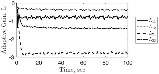
Figure 8. AdaptiveGain $L\left(t\right)$ approaching a steady state with the use of a fixed gain and $aL\ne 0$.

3.3.3. Kalman–Bucy Filter–Kalman Filter in Continuous Time

In both Section 3.3.1 and Section 3.3.2, the error dynamics for the proposed adaptive state estimator are presented in two variations: without and with the feedback filter. This section depicts the error dynamics without implementing the adaptive estimator; the fixed gain value $\left(K\right)$ in the estimator remains unchanged compared to Section 3.3.1 and Section 3.3.2. As illustrated in Figure 9a,b, the lack of adaptation in the reference model results in significantly larger internal and external estimation errors compared to those observed when the adaptive control scheme is applied.

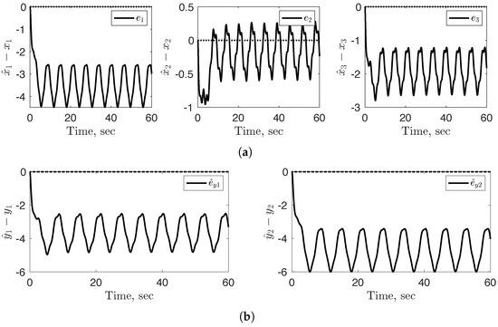
Figure 9. Sub-figures (a,b) illustrate the internal state error $\left(e_x\right)$ and external state error $\left({\widehat{e}}_y\right)$, respectively, in the absence of reference model updating to account for changes in the true system health. Both error states exhibit significantly larger estimation errors compared to their counterparts obtained using the adaptive scheme.

4. Discussion

The theorem and illustrative example presented in this paper pertain to global LTI systems. However, since many real-world problems are inherently non-linear, the proposed theorem can also be applied to any local linear approximation of a non-linear system, provided that the assumptions and constraints of both the theorem and the linear approximation are met.

While there are theoretical hard constraints, such as that the decomposition of the true plant must follow $A=A_m+B{L}_{*}C$, these constraints are essential for the proof. Future research could explore ways to relax or circumvent these constraints. Moreover, the decomposition of the true plant $\left(A\right)$ may appear unrealistic for many applications; however, if additional actuators and sensors can be incorporated, thereby rendering the true system over-controllable and over-observable, the feasibility of satisfying the decomposition improves. If adding extra sensors is not an option, employing sensor blending or fusion techniques can aid in meeting the decomposition constraints. Sensor blending or fusion techniques are routinely used in signal processing and state estimation applications [22,23]. Although the necessary decomposition of the true system may initially seem restrictive, given an initial model, the theory enables the error states to converge to a neighborhood around zero, regardless of how large or small the values inside $L_{*}$ are. In practice, numerical limitations may exist in the theorem due to the integration of large errors.

Knowledge of the input and output matrices $\{B,C\}$ is essential for the theoretical development and stability proof. This assumption is common in control design as the input matrix $\left(B\right)$ denotes how the input $\left(u\right)$ influences the system dynamics, and the output matrix $\left(C\right)$ specifies the linear combination of the internal states that are measured-observed. Practical issues may arise if these matrices degrade over time or with use, but those types of degradation are outside the scope of this work.

The current design of the proposed estimator is non-invasive, meaning that none of the estimated states are fed back into the true system. As a result, the estimation scheme can be implemented without any risk of harming the true system. One potential application of the estimator is to operate in conjunction with governing inputs that regulate the true system response. This parallel implementation can assist in monitoring or refining the equations of motion that govern the true system dynamics. A significant change in a specific constitutive constant or internal interaction could alert an operator to inspect a particular area for potential failures or indicate that a component within the system needs to be replaced.

The theorem only guarantees an asymptotic convergence of the error states, which may limit the potential real-time, online use. In principle, the theorem can be applied to both fast and slow dynamics systems. However, several factors may limit the practical implementation of the theorem. These include the accuracy of the initial system model, the operational range of the true system, and whether the estimated states are used in control design. For instance, consider a scenario involving a mechatronic system with a poorly identified initial model, where the goal is trajectory tracking using the estimated states. In such cases, the implementation of the proposed theorem may not be feasible for online use. However, the scenario can still be evaluated in an offline setting to assess its performance. Additionally, incorporating a fixed gain term $\left(K\right)$ in the estimator can aid or hinder state estimation, depending on how the fixed gain term is tuned. However, the proof indicates that the inclusion of this fixed term is not necessary for the state estimation error to converge to a neighborhood around zero.

The outlined theorem in this paper pertains to accounting for model uncertainty and stochastic noise. If noise term is removed $(v_x=0)$, the need for the robust analysis subsides. From here, our previous finding, outlined in [16], can be used to ensure $\{e_x,{\widehat{e}}_y\}\underset{t\to \infty }{\to }0$. However, the result in [16] can be extended by considering the control law defined in Equation (18), which truncates the Lyapunov analysis expressed in Equation (32) to the following:

$$\begin{array}{cc}\hfill {\dot{V}}_{eL}+2a{V}_{eL}& \le a\left|\mathrm{tr}\right(L_{*}{\gamma }_y^{-1}∆L^{†}\left)\right|\hfill \\ & \le a\underset{={\displaystyle \frac{M_L}{a}}}{\underbrace{\mathrm{tr}(L_{*}^{†}{L}_{*}){)}^{{\displaystyle \frac{1}{2}}}\mathrm{tr}{\left({\gamma }_y\right)}^{{\displaystyle \frac{1}{2}}}}}{\left(2V_{eL}\right)}^{{\displaystyle \frac{1}{2}}}\hfill \\ \hfill & =M_L{\left(2V_{eL}\right)}^{{\displaystyle \frac{1}{2}}},\hfill \end{array}$$

(81)

where $M_L$ is a scalar value greater than zero $(M_L>0)$. Following a similar analysis described earlier in this text, the error state norm is bounded by the following radius of convergence, denoted as $R_{*}$:

$$\underset{t\to \infty }{\lim \sup }\parallel e_x\parallel \le {\displaystyle \frac{M_L}{a\sqrt{{\lambda }_{\min }\left(P_x\right)}}}\equiv R_{*}.$$

(82)

where $R_{*}$ represents a radius around a neighborhood of zero.

5. Conclusions

The true system is influenced by stochastic variations and health changes, resulting in alterations in internal interactions and constitutive constants. If these health changes are not considered, discrepancies may arise between the true system and the reference model. The proposed control scheme addresses these issues by updating the reference model utilizing the input and output of the true system. The stability proof ensures that both the internal and external error states will converge within a defined radius around zero. The size of this radius of convergence is contingent upon the extent of the stochastic variations. A potential application of the estimator is to operate in parallel with the system inputs that regulate the response. This parallel configuration can assist in monitoring the health status of the true system, potentially alerting operators when specific internal interactions or constitutive parameters deviate from their nominal values. Future work will focus on relaxing certain Lyapunov-based stability constraints—most notably, the requirement for a specific decomposition of the true plant.

Appendix A.1. Defining the True System Plant

Recall for the adaptive estimator to be utilized, the true plant must follow a specific decomposition: $A=A_m+B{L}_{*}C$. In this example, consider an alternative value for $L_{*}$ given by the following:

$$L_{*}=\left[\begin{array}{cc}-74& 20\\ -6& -50\end{array}\right].$$

(A1)

Therefore, the true plant can be represented as follows:

$$A=\left[\begin{array}{ccc}-70& 2& -14.5\\ -11.1& -1& -46.3\\ -28& 2& -139\end{array}\right],$$

(A2)

with the eigenvalues of the true plant $\left(A\right)$ are given by $\sigma \left\{A\right\}\approx \{-1.72,-64.70,-143.6\}$. Note the dependencies between the model and true plant, as defined in Equation (72) and Equation (A2), respectively. For reference, the eigenvalues of the model plant $\left(A_m\right)$ are as follows: $\sigma \left\{A_m\right\}=\{-1,-3,-5\}$.

Appendix A.2. Adaptive Control Scheme Without a Feedback Filter (aL = 0) and Without a Fixed Gain (K = 0)

The control scheme illustrated in Figure 1 is implemented without a fixed gain $(K=0)$ and the adaptive law without the feedback filter $(aL=0)$, as described in Equation (56). Additionally, the interaction turning term $\left({\gamma }_y\right)$ and the input $\left(u\right)$ remain the same from the previous example.

As illustrated in Figure A1 and Figure A2, both internal and external errors converge to a radius around zero. Due to the theorem only guaranteeing asymptotic convergence and the relatively large discrepancy between the initial model and the true system, it does take a relatively significant time for the error states to approach zero. Nonetheless, the model is updated so the error states converge to a radius around zero.

As discussed in the main text, if there is a large discrepancy between the model and the true system, this theorem may not be realistic in an online setting for fast dynamic systems. This is imparted by the time required for the error states to approach zero can be substantial. Conversely, the theorem could be beneficial offline, where extended time frames can be simulated quickly.

Furthermore, due to the true system having eigenvalues with large negative real parts, the true system response has a smaller magnitude than the previous example using the same input. Consequently, applying the same input leads to slower observable error decay. For this specific case, increasing the magnitude of the input scales the true system’s response accordingly, allowing the adaptive estimator to adjust rapidly and causing the error to subside faster.

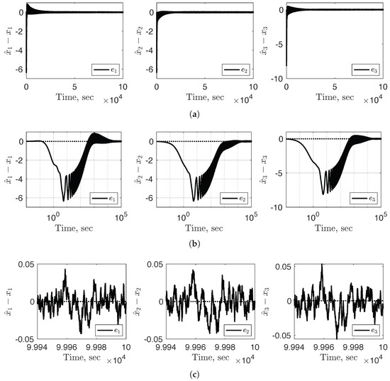
Figure A1. Sub-figures (a–c) illustrate the internal state error $\left(e_x\right)$ converging to zero over varying time scales. Due to the relatively large discrepancies between the model and the true plant, the internal error requires a significant amount of time to converge to a small neighborhood around zero. The implemented control scheme uses neither a fixed gain $(K=0)$ nor the feedback filter on the adaptive estimator law $(aL=0)$.

Although there exists variability in the estimated L’s data as time approaches infinity, as shown in Figure A3, the last 20 s of simulated data was averaged, denoted by $L_{avg}$, resulting in the following:

$$L_{avg}\approx \left[\begin{array}{cc}-74.05& 19.96\\ -4.64& -48.45\end{array}\right].$$

(A3)

Therefore, the estimated plant $\left(A_{avg}\right)$ can be expressed as follows:

$$A_{avg}\approx \left[\begin{array}{ccc}-67.45& 2& -12.75\\ -11.16& -1& -46.34\\ -28.16& 2& -139.13\end{array}\right],$$

(A4)

where the eigenvalues of $A_{avg}$ follows: $\sigma \left\{A_{avg}\right\}=\{-1.72,-62.91,-142.95\}$. Compare the similarities between the true and estimated plant, denoted by Equations (A2) and (A4), respectively.

This example illustrates that model uncertainty can be either local or global. As long as the uncertainty adheres to the specified decomposition, the error states can be shown to converge to the neighborhood around zero. Furthermore, the decay of the error states is influenced by the true system input, emphasizing the role of excitation in the adaptation process.

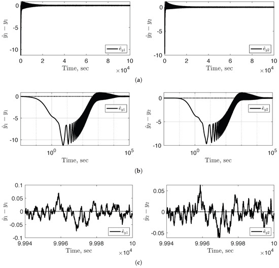
Figure A2. Sub-figures (a–c) illustrate the external state error $\left({\widehat{e}}_y\right)$ converging to zero over varying time scales.

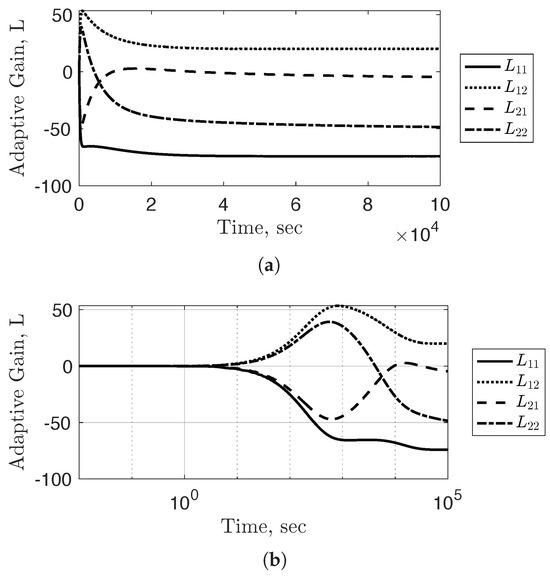
Figure A3. Sub-figures (a,b) illustrated the Adaptive Gain $L\left(t\right)$ converging to $L_{*}$ without the use of the fixed gain $(K=0)$ and $aL=0$, across different time scales.

References

- Cook, R.G.; Palacios, R.; Goulart, P. Robust gust alleviation and stabilization of very flexible aircraft. AIAA J. 2013, 51, 330–340. [Google Scholar] [CrossRef]
- Von Karman, T. Compressibility effects in aerodynamics. J. Spacecr. Rocket. 2003, 40, 992–1011. [Google Scholar] [CrossRef]
- Chen, S.; Gojon, R.; Mihaescu, M. High-temperature effects on aerodynamic and acoustic characteristics of a rectangular supersonic jet. In Proceedings of the 2018 AIAA/CEAS Aeroacoustics Conference, Atlanta, Georgia, 25–29 June 2018; p. 3303. [Google Scholar]
- Balas, M.; Fuentes, R.; Erwin, R. Adaptive control of persistent disturbances for aerospace structures. In Proceedings of the AIAA Guidance, Navigation, and Control Conference and Exhibit, Monterey, CA, USA, 5–8 August 2000; p. 3952. [Google Scholar]
- Fuentes, R.J.; Balas, M.J. Direct adaptive disturbance accommodation. In Proceedings of the 39th IEEE Conference on Decision and Control (Cat. No. 00CH37187), Sydney, NSW, Australia, 12–15 December 2000; Volume 5, pp. 4921–4925. [Google Scholar]
- Wang, N.; Wright, A.D.; Balas, M.J. Disturbance accommodating control design for wind turbines using solvability conditions. J. Dyn. Syst. Meas. Control 2017, 139, 041007. [Google Scholar] [CrossRef]
- Chen, J.; Patton, R.J.; Zhang, H.Y. Design of unknown input observers and robust fault detection filters. Int. J. Control 1996, 63, 85–105. [Google Scholar] [CrossRef]
- Guan, Y.; Saif, M. A novel approach to the design of unknown input observers. IEEE Trans. Autom. Control 1991, 36, 632–635. [Google Scholar] [CrossRef]
- Fuentes, R.J.; Balas, M.J. Robust model reference adaptive control with disturbance rejection. In Proceedings of the 2002 American Control Conference (IEEE Cat. No. CH37301), Anchorage, AK, USA, 8–10 May 2002; Volume 5, pp. 4003–4008. [Google Scholar]
- Luenberger, D.G. Observing the State of a Linear System. IEEE Trans. Mil. Electron. 1964, 8, 74–80. [Google Scholar] [CrossRef]
- Luenberger, D. An introduction to observers. IEEE Trans. Autom. Control 1971, 16, 596–602. [Google Scholar] [CrossRef]
- Kalman, R.E. A New Approach to Linear Filtering and Prediction Problems. J. Basic Eng. 1960, 82, 35–45. [Google Scholar] [CrossRef]
- Kalman, R.E.; Bucy, R.S. New Results in Linear Filtering and Prediction Theory. J. Basic Eng. 1961, 83, 95–108. [Google Scholar] [CrossRef]
- Doyle, J.C. A review of μ for case studies in robust control. IFAC Proc. Vol. 1987, 20, 365–372. [Google Scholar] [CrossRef]
- Nagpal, K.M.; Khargonekar, P.P. Filtering and smoothing in an H/sup infinity/setting. IEEE Trans. Autom. Control 1991, 36, 152–166. [Google Scholar] [CrossRef]
- Fuentes, K.; Balas, M.J.; Hubbard, J. A Control Framework for Direct Adaptive Estimation With Known Inputs for LTI Dynamical Systems. In Proceedings of the AIAA SCITECH 2025 Forum, Orlando, FL, USA, 6–10 January 2025; p. 2796. [Google Scholar]
- Griffith, T.; Gehlot, V.P.; Balas, M.J. Robust adaptive unknown input estimation with uncertain system Realization. In Proceedings of the AIAA SCITECH 2022 Forum, San Diego, CA, USA, 3–7 January 2022; p. 611. [Google Scholar]
- Rigatos, G.G. A Derivative-Free Kalman Filtering Approach to State Estimation-Based Control of Nonlinear Systems. IEEE Trans. Ind. Electron. 2012, 59, 3987–3997. [Google Scholar] [CrossRef]
- Jo, N.H.; Seo, J.H. Input output linearization approach to state observer design for nonlinear system. IEEE Trans. Autom. Control 2000, 45, 2388–2393. [Google Scholar] [CrossRef]
- Leith, D.J.; Leithead, W.E. Survey of gain-scheduling analysis and design. Int. J. Control 2000, 73, 1001–1025. [Google Scholar] [CrossRef]
- Balas, M.; Fuentes, R. A non-orthogonal projection approach to characterization of almost positive real systems with an application to adaptive control. In Proceedings of the 2004 American Control Conference, Boston, MA, USA, 30 June 30–2 July 2004; Volume 2, pp. 1911–1916. [Google Scholar]
- Sun, S.L.; Deng, Z.L. Multi-sensor optimal information fusion Kalman filter. Automatica 2004, 40, 1017–1023. [Google Scholar] [CrossRef]
- Wang, S.; Yi, S.; Zhao, B.; Li, Y.; Li, S.; Tao, G.; Mao, X.; Sun, W. Sowing Depth Monitoring System for High-Speed Precision Planters Based on Multi-Sensor Data Fusion. Sensors 2024, 24, 6331. [Google Scholar] [CrossRef] [PubMed]
Disclaimer/Publisher’s Note: The statements, opinions and data contained in all publications are solely those of the individual author(s) and contributor(s) and not of MDPI and/or the editor(s). MDPI and/or the editor(s) disclaim responsibility for any injury to people or property resulting from any ideas, methods, instructions or products referred to in the content. |
© 2025 by the authors. Licensee MDPI, Basel, Switzerland. This article is an open access article distributed under the terms and conditions of the Creative Commons Attribution (CC BY) license (https://creativecommons.org/licenses/by/4.0/).