
Research on Plant Disease and Pest Diagnosis Model Based on Generalized Stochastic Petri Net


Abstract
1. Introduction
2. Early Warning System for Plant Pests and Diseases
2.1. Influence of Environmental Factors
2.2. Pest and Disease Damage and Control
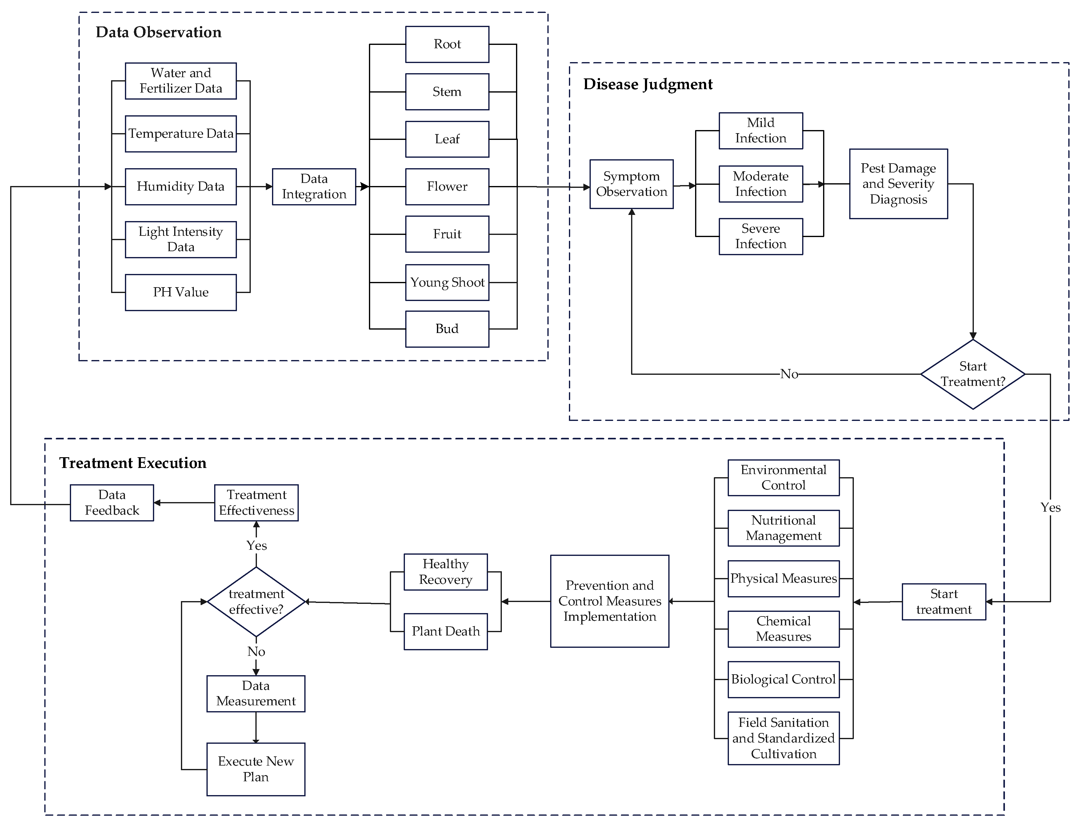
2.3. Establishing a Plant Pest and Disease Early Warning System
3. Generalized Random Petri Net Model for Plant Pest and Disease Spread Diagnosis
3.1. Generalized Stochastic Petri Net
- In GSPN, the system is described as a directed graph consisting of six basic elements, denoted as [22]. These elements are specifically defined as follows:
- is the set of places, representing the various states or conditions in the system. In the plant pest and disease spread diagnosis model, places represent the key states and factors designed in the spread process, such as moisture factor , fertilizer factor , and so on. Here, denotes the number of elements.
- is the set of transitions, triggered based on the conditions defined in . This set includes two types of transitions: Time transitions ,which simulate activities with delays, such as the disease development stages. Instantaneous transitions , , used to represent immediate events, such as the rapid diagnosis of a disease.
- is the set of directed arcs, connecting places and transitions, determining the flow of tokens. represents the input arcs of transitions in the Petri net; represents the output arcs of transitions in the Petri net. The association matrix in the Petri net is defined as . Set has direction, representing the path through which pests and diseases transition from one state to another.is the arc weight function vector, where , represents the capacity of each system transition.
- is the state-marking vector of the Petri net, which represents the possible states of the pest and disease spread system during its dynamic operation by defining the number of tokens in each place. represents the initial marking of the system. If there is no function defined on an arc, the default weight is 1.
- represents the average triggering frequency associated with time transitions [23]. Each is an exponential distribution parameter used to describe the average time interval between the triggers of the corresponding time transition. This allows the model to probabilistically express the occurrence of transitions, with the value for instantaneous transitions defaulting to zero, reflecting their characteristic of occurring immediately with no delay.
3.2. Pest and Disease Spread Evolution Modeling Methods
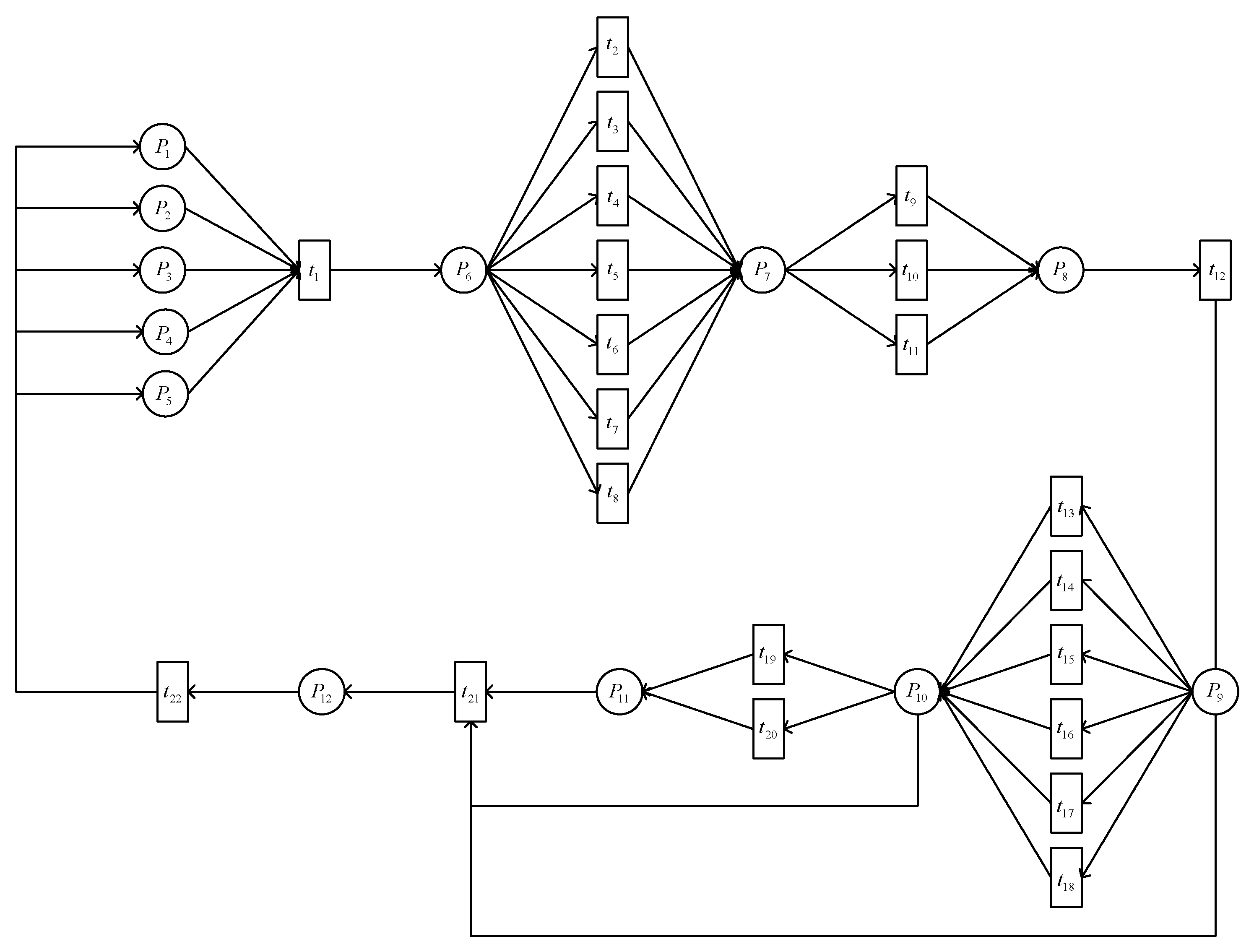
3.3. The GSPN Model for Plant Pest and Disease Spread Evolution
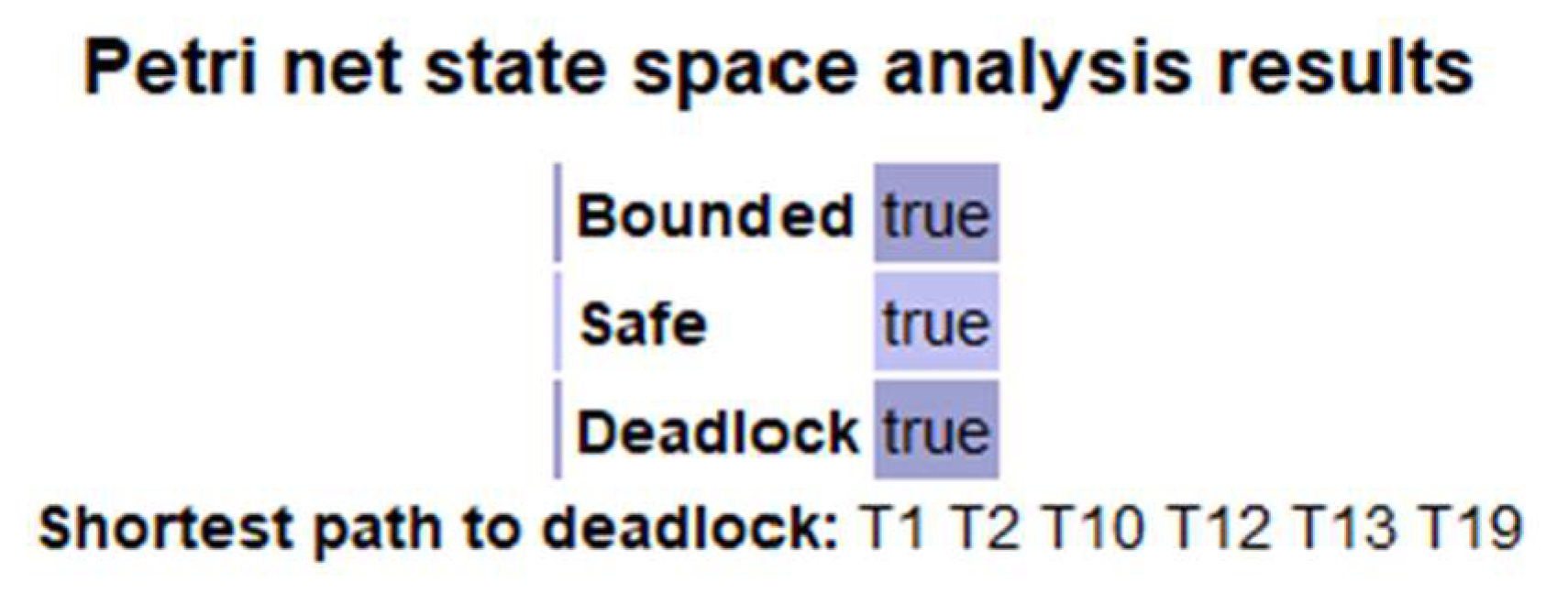
3.4. Stimulation Experiment of the Model
4. Simulation Analysis
4.1. Performance Analysis of Pest and Disease Spread Evolution Process Based on the GSPN Model
4.1.1. Busy Probability of a Place
4.1.2. Place Idle Probability
4.1.3. Transition Utilization Rate
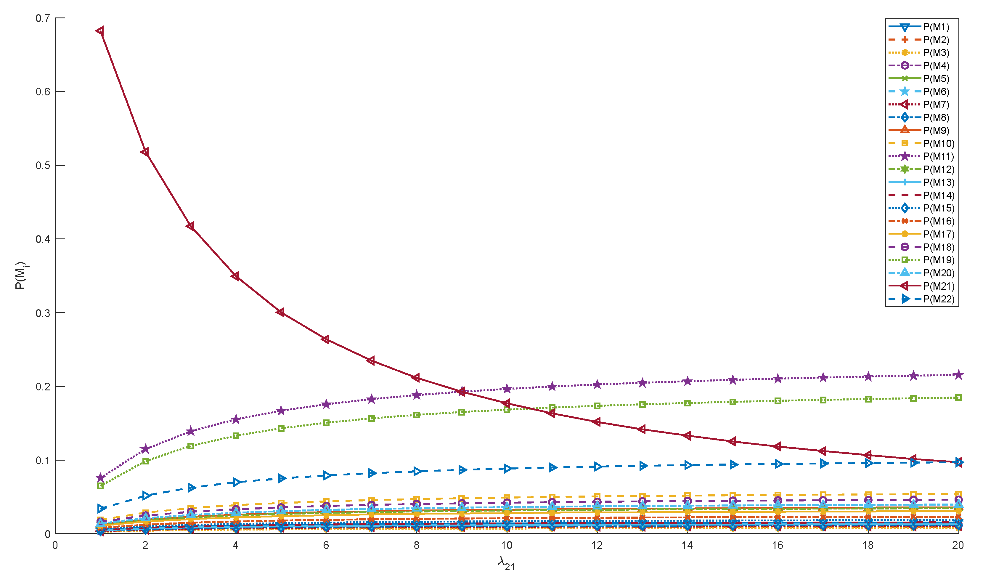
4.2. Stimulation Analysis of the Pest and Disease Diagnosis Model
4.2.1. Data Observation Stage
4.2.2. Disease Judgment Stage
4.2.3. Treatment Execution Stage
5. Case Study
5.1. The GSPN Model for the Spread and Evolution of Grape Downy Mildew
5.2. Verification of the Grape Downy Mildew Pest and Disease Early Warning System
6. Conclusions
Author Contributions
Funding
Institutional Review Board Statement
Informed Consent Statement
Data Availability Statement
Conflicts of Interest
References
- Zou, B.; Mishra, A.K. Modernizing Smallholder Agriculture and Achieving Food Security: An Exploration in Machinery Services and Labor Reallocation in China. Appl. Econ. Perspect. Policy 2024, 46, 1662–1691. [Google Scholar] [CrossRef]
- Corredor-Moreno, P.; Saunders, D.G.O. Expecting the Unexpected: Factors Influencing the Emergence of Fungal and Oomycete Plant Pathogens. New Phytol. 2020, 225, 118–125. [Google Scholar] [CrossRef] [PubMed]
- Prakash, R.M.; Saraswathy, G.P.; Ramalakshmi, G.; Mangaleswari, K.H.; Kaviya, T. Detection of Leaf Diseases and Classification Using Digital Image Processing. In Proceedings of the 2017 International Conference on Innovations in Information, Embedded and Communication Systems (ICIIECS), Coimbatore, India, 17–18 March 2017; pp. 1–4. [Google Scholar]
- Krithika, P.; Veni, S. Leaf Disease Detection on Cucumber Leaves Using Multiclass Support Vector Machine. In Proceedings of the 2017 International Conference on Wireless Communications, Signal Processing and Networking (WiSPNET), Chennai, India, 22–24 March 2017; pp. 1276–1281. [Google Scholar]
- Motie, J.B.; Saeidirad, M.H.; Jafarian, M. Identification of Sunn-Pest Affected (Eurygaster integriceps put.) Wheat Plants and Their Distribution in Wheat Fields Using Aerial Imaging. Ecol. Inform. 2023, 76, 102146. [Google Scholar] [CrossRef]
- Hernández, S.; López, J.L. Uncertainty Quantification for Plant Disease Detection Using Bayesian Deep Learning. Appl. Soft Comput. 2020, 96, 106597. [Google Scholar] [CrossRef]
- Nagasubramanian, K.; Singh, A.K.; Singh, A.; Sarkar, S.; Ganapathysubramanian, B. Usefulness of Interpretability Methods to Explain Deep Learning Based Plant Stress Phenotyping. arXiv 2020. [Google Scholar] [CrossRef]
- Qiu, J.; Lu, X.; Wang, X.; Chen, C.; Chen, Y.; Yang, Y. Research on Image Recognition of Tomato Leaf Diseases Based on Improved AlexNet Model. Heliyon 2024, 10, e33555. [Google Scholar] [CrossRef]
- Fuentes, A.; Yoon, S.; Kim, S.C.; Park, D.S. A Robust Deep-Learning-Based Detector for Real-Time Tomato Plant Diseases and Pests Recognition. Sensors 2017, 17, 2022. [Google Scholar] [CrossRef]
- Szegedy, C.; Liu, W.; Jia, Y.; Sermanet, P.; Reed, S.; Anguelov, D.; Erhan, D.; Vanhoucke, V.; Rabinovich, A. Going Deeper With Convolutions. In Proceedings of the 2015 IEEE Conference on Computer Vision and Pattern Recognition (CVPR), Boston, MA, USA, 7–12 June 2015; pp. 1–9. [Google Scholar]
- Adegun, A.; Viriri, S. Deep Learning Techniques for Skin Lesion Analysis and Melanoma Cancer Detection: A Survey of State-of-the-Art. Artif. Intell. Rev. 2021, 54, 811–841. [Google Scholar] [CrossRef]
- Ahad, M.T.; Li, Y.; Song, B.; Bhuiyan, T. Comparison of CNN-Based Deep Learning Architectures for Rice Diseases Classification. Artif. Intell. Agric. 2023, 9, 22–35. [Google Scholar] [CrossRef]
- Yang, C.-Y.; Lin, Y.-N.; Shen, V.R.L.; Shen, F.H.C.; Lin, Y.-C. Petri Net Modeling and Analysis of an IoT-Enabled System for Real-Time Monitoring of Eggplants. Syst. Eng. 2025, 28, 270–283. [Google Scholar] [CrossRef]
- Geng, X.; Zhu, C.; Zhang, J.; Xiong, Z. Prediction of Soil Fertility Change Trend Using a Stochastic Petri Net. J. Signal Process. Syst. 2021, 93, 285–297. [Google Scholar] [CrossRef]
- Wang, W.; Yang, S.; Zhang, X.; Xia, X. Research on the Smart Broad Bean Harvesting System and the Self-Adaptive Control Method Based on CPS Technologies. Agronomy 2024, 14, 1405. [Google Scholar] [CrossRef]
- Zhang, Y.; Zhang, Y.; Wen, F.; Chung, C.Y.; Tseng, C.-L.; Zhang, X.; Zeng, F.; Yuan, Y. A Fuzzy Petri Net Based Approach for Fault Diagnosis in Power Systems Considering Temporal Constraints. Int. J. Electr. Power Energy Syst. 2016, 78, 215–224. [Google Scholar] [CrossRef]
- Hui, M.; Ni, F.; Liu, W.; Liu, J.; Chen, N.; Zhou, X. SPN-Based Dynamic Risk Modeling of Fire Incidents in a Smart City. Appl. Sci. 2025, 15, 2701. [Google Scholar] [CrossRef]
- Zegordi, S.H.; Davarzani, H. Developing a Supply Chain Disruption Analysis Model: Application of Colored Petri-Nets. Expert Syst. Appl. 2012, 39, 2102–2111. [Google Scholar] [CrossRef]
- Peng, L.; Xie, P.; Tang, Z.; Liu, F. Modeling and Analyzing Transmission of Infectious Diseases Using Generalized Stochastic Petri Nets. Appl. Sci. 2021, 11, 8400. [Google Scholar] [CrossRef]
- Shafik, W.; Tufail, A.; De Silva Liyanage, C.; Apong, R.A.A.H.M. Using Transfer Learning-Based Plant Disease Classification and Detection for Sustainable Agriculture. BMC Plant Biol. 2024, 24, 136. [Google Scholar] [CrossRef]
- Song, Y.; Xu, H.; Fang, D.; Sang, X. Modelling and Analysis of Emergency Scenario Evolution System Based on Generalized Stochastic Petri Net. Systems 2025, 13, 107. [Google Scholar] [CrossRef]
- Chiola, G.; Marsan, M.A.; Balbo, G.; Conte, G. Generalized Stochastic Petri Nets: A Definition at the Net Level and Its Implications. IEEE Trans. Softw. Eng. 1993, 19, 89–107. [Google Scholar] [CrossRef]
- Molloy, M.K. Discrete Time Stochastic Petri Nets. IEEE Trans. Softw. Eng. 1985, 11, 417–423. [Google Scholar] [CrossRef]
- Sun, H.; Liu, J.; Han, Z.; Jiang, J. Stochastic Petri Net Based Modeling of Emergency Medical Rescue Processes during Earthquakes. J. Syst. Sci. Complex. 2021, 34, 1063–1086. [Google Scholar] [CrossRef] [PubMed]
- Ma, Z.; Li, Z.; Giua, A. Design of Optimal Petri Net Controllers for Disjunctive Generalized Mutual Exclusion Constraints. IEEE Trans. Autom. Control 2015, 60, 1774–1785. [Google Scholar] [CrossRef]
- Liu, S.; Li, W.; Gao, P.; Sun, Y. Modeling and Performance Analysis of Gas Leakage Emergency Disposal Process in Gas Transmission Station Based on Stochastic Petri Nets. Reliab. Eng. Syst. Saf. 2022, 226, 108708. [Google Scholar] [CrossRef]
- Dingle, N.J.; Knottenbelt, W.J.; Suto, T. PIPE2: A Tool for the Performance Evaluation of Generalised Stochastic Petri Nets. ACM SIGMETRICS Perform. Eval. Rev. 2009, 36, 34–39. [Google Scholar] [CrossRef]
- Wang, C.; Wang, L.; Su, C.; Jiang, M.; Li, Z.; Deng, J. Modeling and Performance Analysis of Emergency Response Process for Hydrogen Leakage and Explosion Accidents. J. Loss Prev. Process Ind. 2024, 87, 105239. [Google Scholar] [CrossRef]
- Grünig, M.; Razavi, E.; Calanca, P.; Mazzi, D.; Wegner, J.D.; Pellissier, L. Applying Deep Neural Networks to Predict Incidence and Phenology of Plant Pests and Diseases. Ecosphere 2021, 12, e03791. [Google Scholar] [CrossRef]
- Appeltans, S.; Pieters, J.G.; Mouazen, A.M. Detection of Leek White Tip Disease under Field Conditions Using Hyperspectral Proximal Sensing and Supervised Machine Learning. Comput. Electron. Agric. 2021, 190, 106453. [Google Scholar] [CrossRef]
- Alimzhanova, M.; Meirbekov, N.; Syrgabek, Y.; López-Serna, R.; Yegemova, S. Plant- and Microbial-Based Organic Disease Management for Grapevines: A Review. Agriculture 2025, 15, 963. [Google Scholar] [CrossRef]
- Mubeen, I.; Fawzi Bani Mfarrej, M.; Razaq, Z.; Iqbal, S.; Naqvi, S.A.H.; Hakim, F.; Mosa, W.F.A.; Moustafa, M.; Fang, Y.; Li, B. Nanopesticides in Comparison with Agrochemicals: Outlook and Future Prospects for Sustainable Agriculture. Plant Physiol. Biochem. 2023, 198, 107670. [Google Scholar] [CrossRef]
- Sun, Z.-B.; Song, H.-J.; Liu, Y.-Q.; Ren, Q.; Wang, Q.-Y.; Li, X.-F.; Pan, H.-X.; Huang, X.-Q. The Potential of Microorganisms for the Control of Grape Downy Mildew—A Review. J. Fungi 2024, 10, 702. [Google Scholar] [CrossRef]
- GB/T 17980.122-2004; Pesticide-Guidelines for the Field Efficacy Trials (II)—Part 122: Fungicides Against Downy Mildew of Grape. General Administration of Quality Supervision, Inspection and Quarantine of the People’s Republic of China: Beijing, China, 2004.


| C | Disease | C | Moisture | C | Fertilizer | C | Temperature | C | Humidity | C | Light | C | PH Value |
|---|---|---|---|---|---|---|---|---|---|---|---|---|---|
| D1 | Downy Mildew | E1 | Dry | A1 | Excessive Nitrogen Fertilizer | TR1 | 15–20 °C | H1 | High Humidity | L1 | Low Light | PH1 | Alkaline |
| D2 | Powdery Mildew | E2 | Insufficient Water | A2 | Insufficient Fertilization | TR2 | 20–25 °C | H2 | Moderate Humidity | L2 | Moderate Light | PH2 | Neutral |
| D3 | Gray Mold | E3 | Water Excess | A3 | Proper Fertilizer Application | TR3 | 25–30 °C | H3 | Low Humidity | L3 | High Light | PH3 | Acidic |
| … | |||||||||||||
| Dm | Disease m | Ea | Moisture Condition a | Ab | Fertilization Status b | TRc | Temperature Condition c | Hd | Humidity Condition d | Le | Light Condition e | PHf | PH Value Condition f |
| C | Disease | C | Moisture | C | Fertilizer | C | Temperature | C | Humidity | C | Light | C | PH Value |
|---|---|---|---|---|---|---|---|---|---|---|---|---|---|
| D4 | Aphids | E1 | Dry | A1 | Excessive Nitrogen Fertilizer | TR1 | 15–20 °C | H1 | High Humidity | L1 | Low Light | PH1 | Alkaline |
| D5 | Borers | E2 | Insufficient Water | A2 | Insufficient Fertilization | TR2 | 20–25 °C | H2 | Moderate Humidity | L2 | Moderate Light | PH2 | Neutral |
| D6 | Red Spider Mite | E3 | Water Excess | A3 | Proper Fertilizer Application | TR3 | 25–30 °C | H3 | Low Humidity | L3 | High Light | PH3 | Acidic |
| … | |||||||||||||
| Dn | Disease n | Ea | Moisture Condition a | Ab | Fertilization Status b | TRc | Temperature Condition c | Hd | Humidity Condition d | Le | Light Condition e | PHf | PH value Condition f |
| C | Root | C | Stem | C | Leaf | C | Flower | C | Fruit | C | Young Shoot | C | Bud | C | Control Measures |
|---|---|---|---|---|---|---|---|---|---|---|---|---|---|---|---|
| R1 | No | S1 | Disease Spots | Y1 | Abscise | K1 | Mold Layer | FR1 | Poor | NS1 | Death | B1 | Mold Layer | C1 | Environmental Control |
| R2 | Indirect | S2 | Powder Coating | Y2 | Dried | K2 | Disease Spots | FR2 | Rot | NS2 | Restricted Growth | B2 | Spots Appear | C2 | Nutritional Management |
| R3 | Attached | S3 | Pest | Y3 | Disease Spots | K3 | Death | FR3 | Indirect | NS3 | Disease Spots | B3 | Obstruction | C3 | Nutritional Management |
| …… | |||||||||||||||
| Rg | Root g | Sh | Stem h | Yj | Leaf j | Kk | Flower k | FRl | Fruit l | NSo | Young Shoot o | Bp | Bud p | Cq | Control Measures q |
| Places | Meaning of Places | Transitions | Meaning of Transitions |
|---|---|---|---|
| P1 | Water and Fertilizer Data | t1 | Information Filtering |
| P2 | Temperature Data | t2 | Root Symptom Observation |
| P3 | Humidity Data | t3 | Stem Symptom Observation |
| P4 | Light Data | t4 | Leaf Symptom Observation |
| P5 | pH Value | t5 | Flower Symptom Observation |
| P6 | Data Integration | t6 | Fruit Symptom Observation |
| P7 | Infection Severity Assessment | t7 | Young Shoot Symptom Observation |
| P8 | Invasion Severity Assessment | t8 | Bud Symptom Observation |
| P9 | Control Method Decision | t9 | Mild Infection |
| P10 | Implementation of Control Measures | t10 | Moderate Infection |
| P11 | Data Monitoring | t11 | Severe Infection |
| P12 | End of Treatment | t12 | Reaching Treatment Standards |
| t13 | Environmental Control | ||
| t14 | Nutritional Management | ||
| t15 | Physical Methods | ||
| t16 | Chemical Methods | ||
| t17 | Biological Control | ||
| t18 | Field Cleanliness and Standard Cultivation | ||
| t19 | Recovery of Health | ||
| t20 | Plant Death | ||
| t21 | Treatment Effectiveness Assessment | ||
| t22 | Data Feedback |
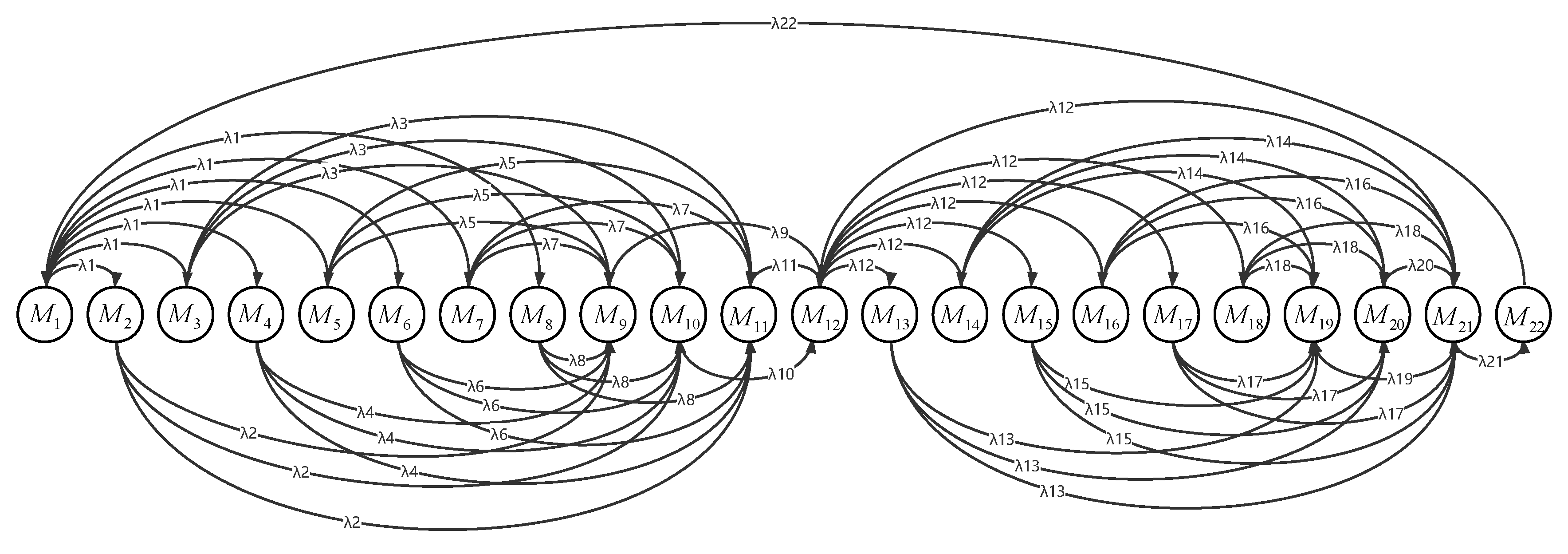
| Data Stage | λ Value | Specific Value | Source |
|---|---|---|---|
| Data Observation Stage | λ1 | 18 | Grünig et al., Experimental Data |
| λ2 | 10 | Expert Recommendations | |
| λ3 | 12 | Expert Recommendations | |
| λ4 | 8 | Expert Recommendations | |
| λ5 | 7 | Expert Recommendations | |
| λ6 | 6 | Expert Recommendations | |
| λ7 | 9 | Expert Recommendations | |
| λ8 | 8 | Expert Recommendations | |
| Disease Assessment Stage | λ9 | 18 | Appeltans et al. |
| λ10 | 8 | Appeltans et al. | |
| λ11 | 3 | Appeltans et al. | |
| λ12 | 8 | Expert Recommendations, Experimental Data | |
| Treatment Execution Stage | λ13 | 7 | Alimzhanova et al. |
| λ14 | 6 | Alimzhanova et al. | |
| λ15 | 5 | Alimzhanova et al. | |
| λ16 | 4 | Alimzhanova et al. | |
| λ17 | 3 | Mubeen et al. | |
| λ18 | 2 | Mubeen et al. | |
| λ19 | 3 | Expert Recommendations | |
| λ20 | 14 | Expert Recommendations | |
| λ21 | 9 | Expert Recommendations, Experimental Data | |
| λ22 | 20 | Expert Recommendations, Experimental Data |
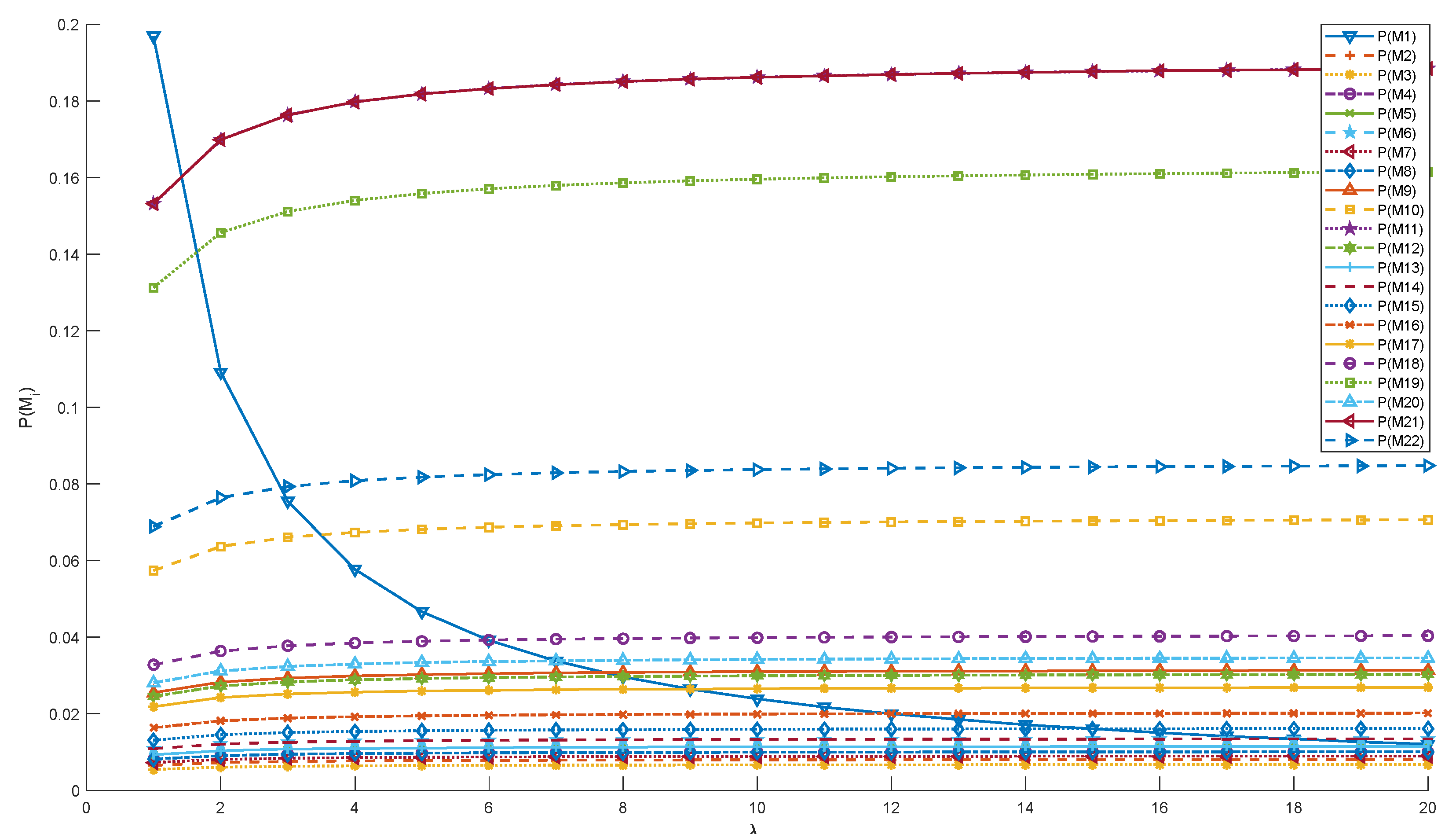
| Mark | Steady-State Probability | Mark | Steady-State Probability |
|---|---|---|---|
| P(M1) | 0.013443 | P(M12) | 0.030248 |
| P(M2) | 0.008066 | P(M13) | 0.011523 |
| P(M3) | 0.006722 | P(M14) | 0.013443 |
| P(M4) | 0.010083 | P(M15) | 0.016132 |
| P(M5) | 0.011523 | P(M16) | 0.020165 |
| P(M6) | 0.013443 | P(M17) | 0.026887 |
| P(M7) | 0.008962 | P(M18) | 0.04033 |
| P(M8) | 0.010083 | P(M19) | 0.161321 |
| P(M9) | 0.031368 | P(M20) | 0.034569 |
| P(M10) | 0.070578 | P(M21) | 0.188208 |
| P(M11) | 0.188208 | P(M22) | 0.084694 |
| P1 | P2 | P3 | P4 | P5 | P6 | P7 | P8 | P9 | P10 | P11 | P12 | |
|---|---|---|---|---|---|---|---|---|---|---|---|---|
| M1 | 1 | 1 | 1 | 1 | 1 | 0 | 0 | 0 | 0 | 0 | 0 | 0 |
| M2 | 0 | 0 | 0 | 0 | 0 | 1 | 0 | 0 | 0 | 0 | 0 | 0 |
| M3 | 0 | 0 | 0 | 0 | 0 | 0 | 1 | 0 | 0 | 0 | 0 | 0 |
| M4 | 0 | 0 | 0 | 0 | 0 | 0 | 1 | 0 | 0 | 0 | 0 | 0 |
| M5 | 0 | 0 | 0 | 0 | 0 | 0 | 1 | 0 | 0 | 0 | 0 | 0 |
| M6 | 0 | 0 | 0 | 0 | 0 | 0 | 1 | 0 | 0 | 0 | 0 | 0 |
| M7 | 0 | 0 | 0 | 0 | 0 | 0 | 1 | 0 | 0 | 0 | 0 | 0 |
| M8 | 0 | 0 | 0 | 0 | 0 | 0 | 1 | 0 | 0 | 0 | 0 | 0 |
| M9 | 0 | 0 | 0 | 0 | 0 | 0 | 1 | 0 | 0 | 0 | 0 | 0 |
| M10 | 0 | 0 | 0 | 0 | 0 | 0 | 0 | 1 | 0 | 0 | 0 | 0 |
| M11 | 0 | 0 | 0 | 0 | 0 | 0 | 0 | 1 | 0 | 0 | 0 | 0 |
| M12 | 0 | 0 | 0 | 0 | 0 | 0 | 0 | 1 | 0 | 0 | 0 | 0 |
| M13 | 0 | 0 | 0 | 0 | 0 | 0 | 0 | 0 | 1 | 0 | 0 | 0 |
| M14 | 0 | 0 | 0 | 0 | 0 | 0 | 0 | 0 | 0 | 1 | 0 | 0 |
| M15 | 0 | 0 | 0 | 0 | 0 | 0 | 0 | 0 | 0 | 1 | 0 | 0 |
| M16 | 0 | 0 | 0 | 0 | 0 | 0 | 0 | 0 | 0 | 1 | 0 | 0 |
| M17 | 0 | 0 | 0 | 0 | 0 | 0 | 0 | 0 | 0 | 1 | 0 | 0 |
| M18 | 0 | 0 | 0 | 0 | 0 | 0 | 0 | 0 | 0 | 1 | 0 | 0 |
| M19 | 0 | 0 | 0 | 0 | 0 | 0 | 0 | 0 | 0 | 1 | 0 | 0 |
| M20 | 0 | 0 | 0 | 0 | 0 | 0 | 0 | 0 | 0 | 0 | 1 | 0 |
| M21 | 0 | 0 | 0 | 0 | 0 | 0 | 0 | 0 | 1 | 1 | 1 | 0 |
| M22 | 0 | 0 | 0 | 0 | 0 | 0 | 0 | 0 | 0 | 0 | 0 | 1 |
| Place | Busy Probability | Place | Busy Probability |
|---|---|---|---|
| M1 | 0.013443 | M7 | 0.092184 |
| M2 | 0.013443 | M8 | 0.289034 |
| M3 | 0.013443 | M9 | 0.199731 |
| M4 | 0.013443 | M10 | 0.466486 |
| M5 | 0.013443 | M11 | 0.222777 |
| M6 | 0.008066 | M12 | 0.084694 |
| Place | Idle Probability | Place | Idle Probability |
|---|---|---|---|
| M1 | 0.986557 | M7 | 0.907816 |
| M2 | 0.986557 | M8 | 0.710966 |
| M3 | 0.986557 | M9 | 0.800269 |
| M4 | 0.986557 | M10 | 0.533514 |
| M5 | 0.986557 | M11 | 0.777223 |
| M6 | 0.991934 | M12 | 0.915306 |
| Transition | Utilization Rate | Transition | Utilization Rate |
|---|---|---|---|
| t1 | 0.013443 | t12 | 0.289034 |
| t2 | 0.008066 | t13 | 0.011523 |
| t3 | 0.008066 | t14 | 0.011523 |
| t4 | 0.008066 | t15 | 0.011523 |
| t5 | 0.008066 | t16 | 0.011523 |
| t6 | 0.008066 | t17 | 0.011523 |
| t7 | 0.008066 | t18 | 0.011523 |
| t8 | 0.008066 | t19 | 0.278278 |
| t9 | 0.092184 | t20 | 0.278278 |
| t10 | 0.092184 | t21 | 0.188208 |
| t11 | 0.092184 | t22 | 0.084694 |
| Severity Level | Description |
|---|---|
| Mild Infection | Lesions occupy less than 25% of the leaf area |
| Moderate Infection | Lesions occupy 25% to 75% of the leaf area |
| Severe Infection | Lesions occupy more than 75% of the leaf area |
| Date | P(M12) | Detailed Disease Description | Warning Level |
|---|---|---|---|
| 10 April | 0.002 | Small, translucent spots appear on the front side of the leaves; under high humidity, mold is visible; lesion edges are unclear. | Blue Warning |
| 11 April | 0.004 | Lesions begin to turn yellow and gradually take on a circular or irregular shape; a small amount of white mold appears on the leaf underside. | Blue Warning |
| 18 April | 0.007 | Lesions expand; under high humidity, mold increases significantly; infected leaves begin to wither, affecting grape photosynthesis. | Blue Warning |
| 22 April | 0.012 | Lesions merge; mold spreads further with increased humidity; fruits begin to show signs of mold infection, affecting fruit development. | Yellow Warning |
| 26 April | 0.014 | Lesions have extensively expanded; mold covers most leaves; some fruits show severe rot, impacting yield. | Yellow Warning |
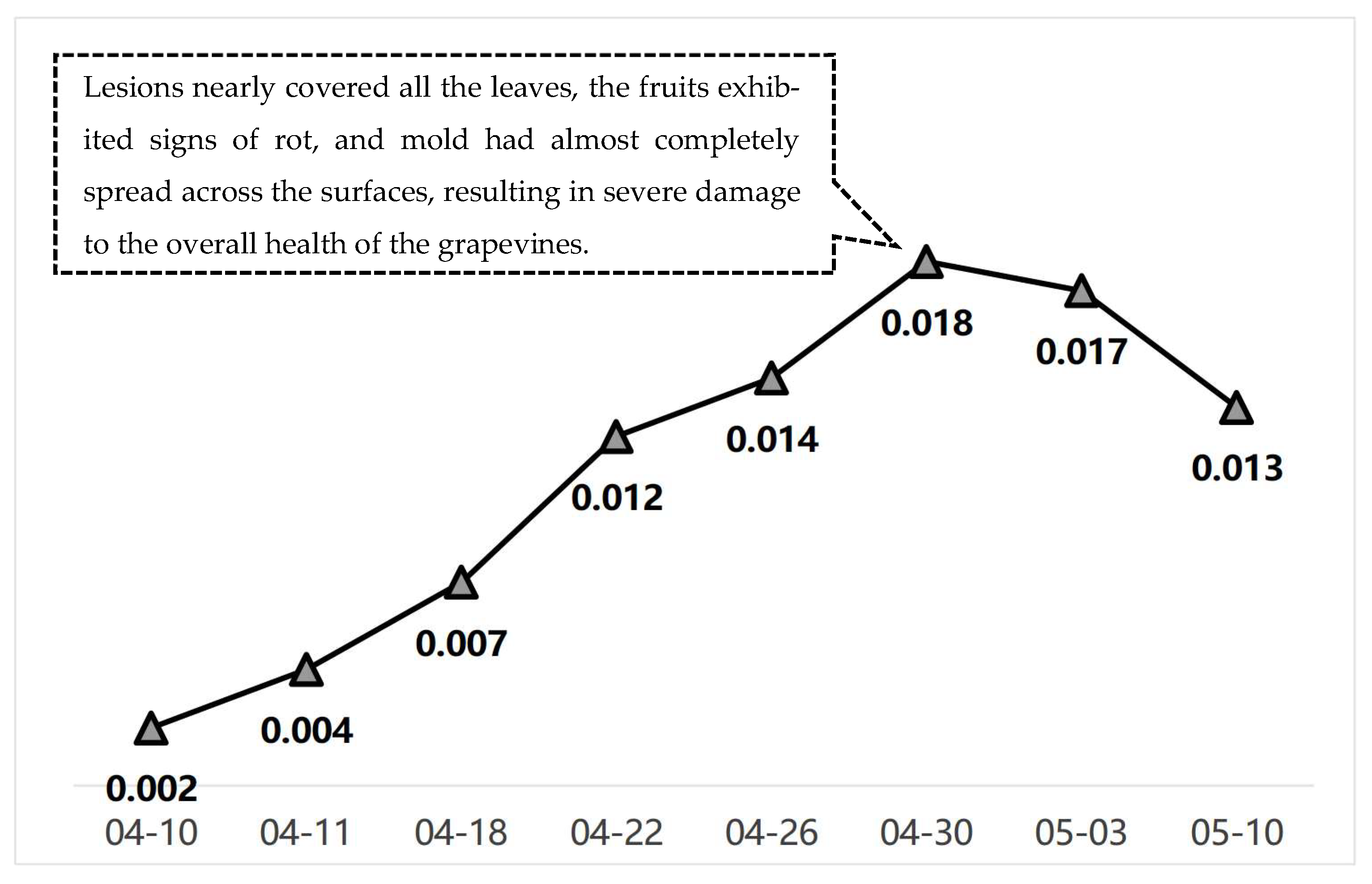
| 30 April | 0.018 | Lesions nearly cover all leaves; fruits rot; mold almost fully covers surfaces, causing severe damage to grapevine health. | Red Warning |
| 3 May | 0.017 | Lesions decrease; some leaves recover, but mold persists; fruit conditions improve somewhat but full recovery has not yet occurred. | Yellow Warning |
| 10 May | 0.013 | Most mold disappears; lesion area gradually reduces; grapevines begin to recover and resume growth; further management is still required. | Yellow Warning |
Disclaimer/Publisher’s Note: The statements, opinions and data contained in all publications are solely those of the individual author(s) and contributor(s) and not of MDPI and/or the editor(s). MDPI and/or the editor(s) disclaim responsibility for any injury to people or property resulting from any ideas, methods, instructions or products referred to in the content. |
© 2025 by the authors. Licensee MDPI, Basel, Switzerland. This article is an open access article distributed under the terms and conditions of the Creative Commons Attribution (CC BY) license (https://creativecommons.org/licenses/by/4.0/).
Share and Cite
Ran, W.; Tang, Q. Research on Plant Disease and Pest Diagnosis Model Based on Generalized Stochastic Petri Net. Appl. Sci. 2025, 15, 6656. https://doi.org/10.3390/app15126656
Ran W, Tang Q. Research on Plant Disease and Pest Diagnosis Model Based on Generalized Stochastic Petri Net. Applied Sciences. 2025; 15(12):6656. https://doi.org/10.3390/app15126656
Chicago/Turabian StyleRan, Wenxue, and Qilian Tang. 2025. "Research on Plant Disease and Pest Diagnosis Model Based on Generalized Stochastic Petri Net" Applied Sciences 15, no. 12: 6656. https://doi.org/10.3390/app15126656
APA StyleRan, W., & Tang, Q. (2025). Research on Plant Disease and Pest Diagnosis Model Based on Generalized Stochastic Petri Net. Applied Sciences, 15(12), 6656. https://doi.org/10.3390/app15126656