Article

A Bidirectional Cross Spatiotemporal Fusion Network with Spectral Restoration for Remote Sensing Imagery

1
School of Geophysics and Geomatics, China University of Geosciences, Wuhan 430074, China
2
Institute of New Energy Equipment, Zhejiang College of Security Technology, Wenzhou 325000, China
3
Wenzhou Future City Research Institute, Wenzhou 325000, China
4
Wenzhou Collaborative Innovation Center for Space-Borne, Airborne and Ground Monitoring Situational Awareness Technology, Wenzhou 325000, China
*
Author to whom correspondence should be addressed.
Appl. Sci. 2025, 15(12), 6649; https://doi.org/10.3390/app15126649
Submission received: 29 April 2025 / Revised: 6 June 2025 / Accepted: 11 June 2025 / Published: 13 June 2025
(This article belongs to the Section Earth Sciences)

Abstract

:
Existing deep learning-based spatiotemporal fusion (STF) methods for remote sensing imagery often focus exclusively on capturing temporal changes or enhancing spatial details while failing to fully leverage spectral information from coarse images. To address these limitations, we propose a Bidirectional Cross Spatiotemporal Fusion Network with Spectral Restoration (BCSR-STF). The network integrates temporal and spatial information using a Bidirectional Cross Fusion (BCF) module and restores spectral fidelity through a Global Spectral Restoration and Feature Enhancement (GSRFE) module, which combines Adaptive Instance Normalization and spatial attention mechanisms. Additionally, a Progressive Spatiotemporal Feature Fusion and Restoration (PSTFR) module employs multi-scale iterative optimization to enhance the interaction between high- and low-level features. Experiments on three datasets demonstrate the superiority of BCSR-STF, achieving significant improvements in capturing seasonal variations and handling abrupt land cover changes compared to state-of-the-art methods.

1. Introduction

Spatiotemporal Fusion (STF) integrates remote sensing data from different sensors and time points [1,2,3], aiming to generate time series remote sensing data with high temporal and spatial resolution. STF effectively addresses the trade-off between temporal and spatial resolution in remote sensing imagery, making it widely applicable in areas such as agricultural monitoring [4,5,6], ecosystem dynamics research [7], and urban heat island analysis [8,9]. Traditional methods, including those based on unmixing [10,11,12], weighted functions [13,14,15], Bayesian [16,17], and machine learning techniques [18,19], have established the theoretical foundation for STF. While these methods are simple and unsupervised, their reliance on linear assumptions limits their ability to model complex remote sensing features.
In recent years, deep learning (DL), with its powerful nonlinear modeling capabilities and automated feature learning, has transformed the research paradigm of STF. Convolutional neural networks (CNNs) are the most widely adopted for STF applications among diverse neural network designs. Models such as DCSTFN [20] and EDCSTFN [21] employ fully end-to-end architectures, using separate CNN branches to extract fine and coarse features. Generative adversarial networks (GANs) address the issue of overly smoothed fusion results, often encountered when training solely with CNNs, by leveraging adversarial loss. For example, GAN-STFM [22] integrates conditional GANs and switchable normalization techniques into STF. Similarly, MLFF-GAN [23] incorporates U-Net-like multi-level feature fusion into the GAN framework. Both approaches use CNNs as the backbone for generator and discriminator networks. However, CNNs struggle to capture long-range dependencies in large-scale spatiotemporal data and adapt to significant heterogeneity due to their fixed weight-sharing mechanism. Transformers [24,25], which utilize self-attention mechanisms for dynamic weight adjustment, have been applied to STF to overcome these limitations. For instance, SwinSTFM [26] effectively combines window-based self-attention [27] with linear unmixing theory, significantly improving spatiotemporal feature modeling capabilities. Additionally, several studies combine CNNs and Transformers to exploit their complementary strengths. STF-Trans [28] employs CNNs as shallow feature extractors and Vision Transformers for deep modeling of long-range dependencies. CTSTFM [29] introduces spatial and channel attention modules along with cross-attention mechanisms to achieve efficient feature extraction and fusion.
In addition to the selection and optimization of backbone networks, DL-based STF methods can also be examined in terms of their core tasks: temporal change capture or spatial detail enhancement. DL methods focused on temporal changes primarily analyze the relationship between images captured at different time points. These methods emphasize capturing variation features within time series and constructing fine-grained difference features. Some approaches directly utilize coarse-difference images and fine images as input. For instance, StfNet [30] adds the coarse-difference images and fine images before feeding them into a CNN-based fusion network. Similarly, PDCNN [31] and STFMCNN [32] stack these inputs for processing through the fusion network. DMNet [33], AMNet [34], and STFDSC [35] extract features from input data using CNNs and subsequently stack or sum these features before passing them to the fusion network. Additionally, networks like DCSTFN [20], EDCSTFN [21], and PSTAF-GAN [36] directly process sequential coarse images, employing difference modeling on the extracted coarse features to enhance temporal fusion.
In contrast, DL methods focusing on spatial details emphasize the scale relationship between coarse and fine images captured on the same date. These methods often approach the STF task as a super-resolution (SR) problem, where the resolution of the coarse image is enhanced to generate a high-resolution image with rich details. For example, STFDCNN [37] employs a five-layer super-resolution CNN to model the nonlinear relationship between MODIS and Landsat images, combining high-pass modulation to fully exploit information from the reference image. Furthermore, some STF networks align with reference-based SR tasks. Notable examples include GAN-STFM [22], MCBAM-GAN [38], STF-Trans [28], and CTSTFM [29], which directly input fine images from the reference time and coarse-resolution images from the target time. These approaches achieve high-accuracy spatiotemporal fusion while reducing dependence on the number of input images.
However, in highly heterogeneous regions, particularly when significant land cover changes occur between prediction and reference dates, models face the dual challenge of capturing temporal variations and preserving spatial structures. Some models address this challenge through parallel processing; for instance, DL-SDFM [39] employs dual CNN architectures to independently predict temporal changes and spatial information before fusing them using weighting functions. MTDL-STF [40] utilizes separate SR and STF networks to predict normalized difference vegetation index (NDVI) values along spatial and temporal dimensions, respectively. However, such decoupled approaches often overlook the intricate interdependencies between temporal and spatial scales, resulting in inaccurate mapping of temporal changes across different scales. Furthermore, significant land cover changes imply that the spectral information from the coarse image at the prediction date may be the only reliable source for predicting the spectra of new land cover types. However, most existing methods fail to fully utilize the prior spectral information provided by coarse images, leading to spectral distortion and insufficient consistency in the fusion results.
Based on the above research, a Bidirectional Cross Spatiotemporal Fusion Network with Spectral Restoration (BCSR-STF) is proposed. This framework achieves bidirectional fusion for temporal change modeling (time direction) and detail enhancement modeling (scale direction) through a Progressive Spatiotemporal Feature Fusion and Restoration (PSTFR) module. The PSTFR module incorporates a multi-scale optimization design with local and global attention. At each level, it enables bidirectional spatiotemporal feature interaction across short-range and long-range distances, and it adaptively optimizes the fused features using spectral prior knowledge. The contributions of this work are summarized as follows:
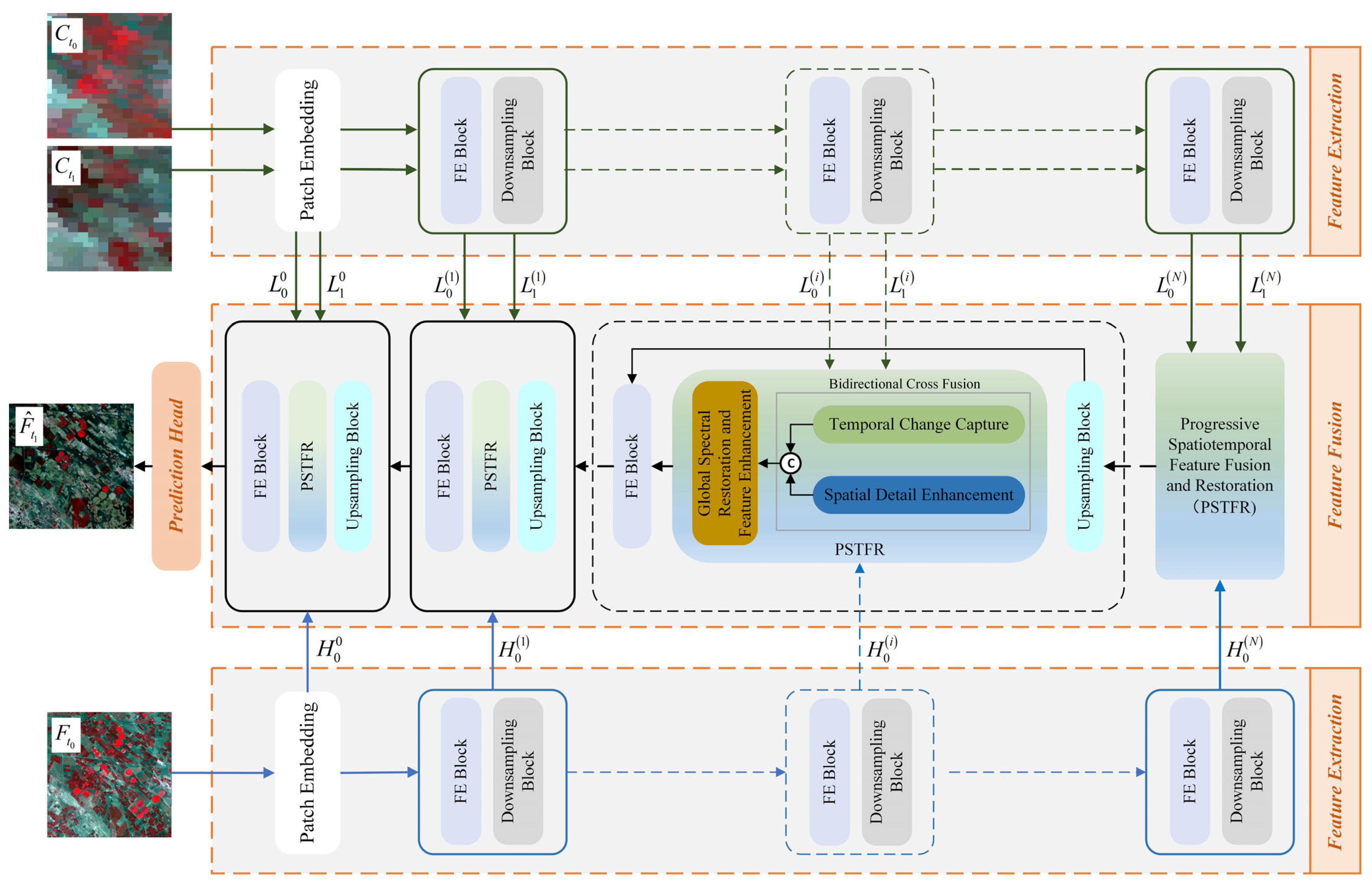
  • An end-to-end BCSR-STF model is proposed. The PSTFR module within BCSR-STF employs multi-scale iterative optimization, enabling effective exchange between high-level and low-level information. The design enhances the model’s capability to address variations in object scale within input images, thereby improving the accuracy of spatiotemporal fusion.
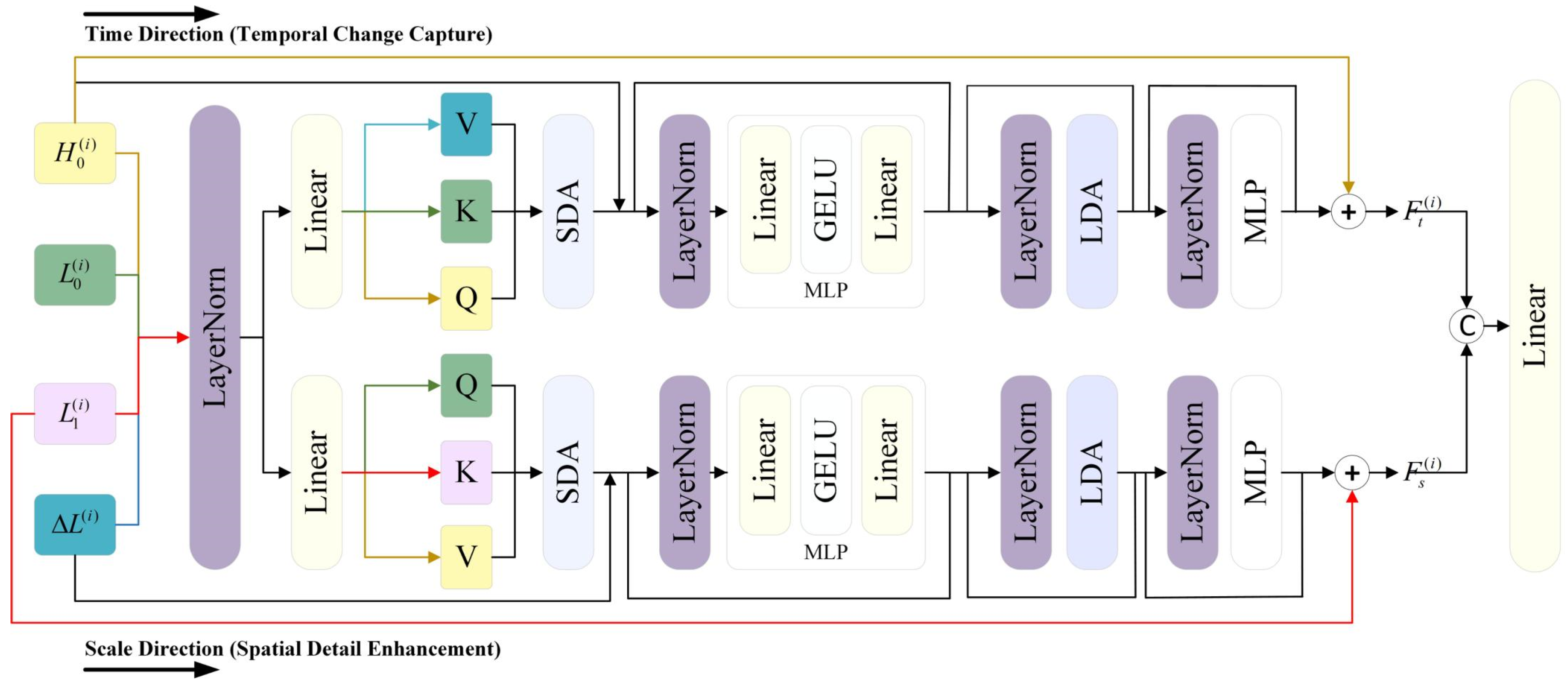
  • A Bidirectional Cross Fusion (BCF) module is designed to leverage the advantages and mitigate the limitations of temporal and scale directions. This module simultaneously considers temporal variations and scale differences, utilizing short-range and long-range attention mechanisms based on the Vision Transformer to enhance interactions between temporal and spatial information, thereby improving fusion accuracy.
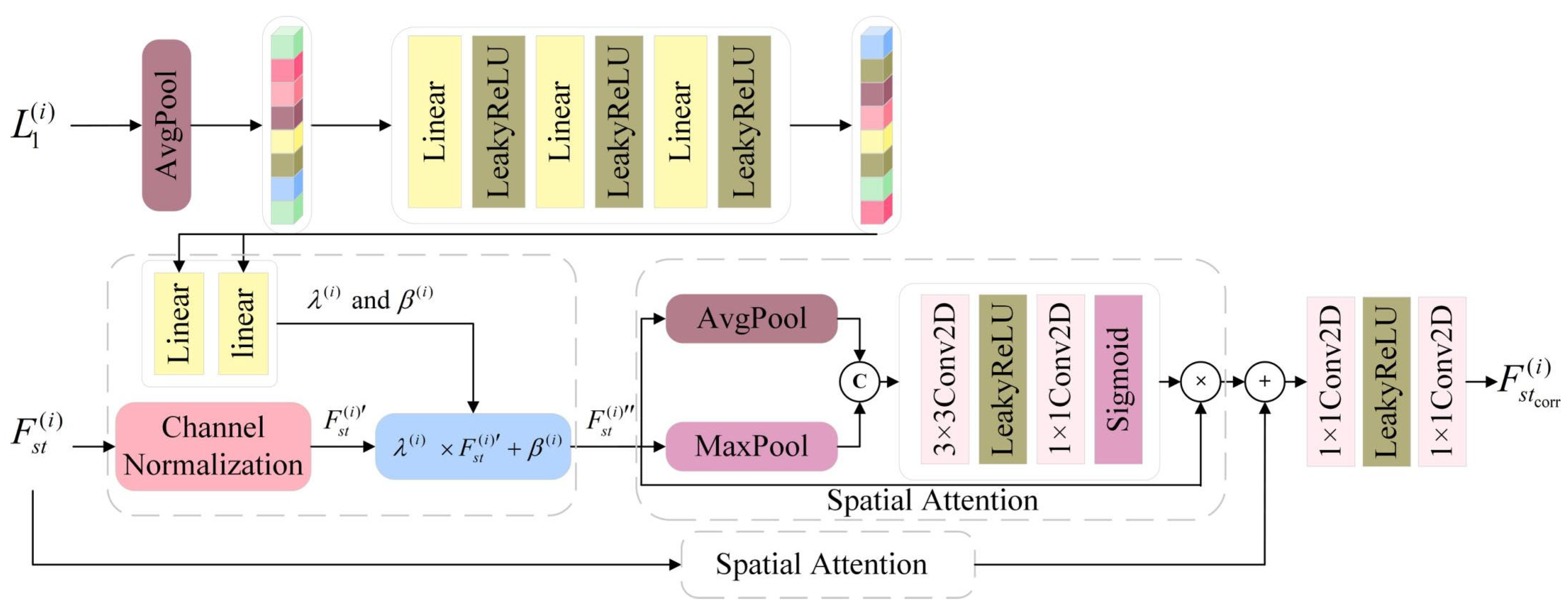
  • The Global Spectral Restoration and Feature Enhancement (GSRFE) module is introduced to restore and enhance spectral information often overlooked in coarse images. By incorporating Adaptive Instance Normalization (AdaIN) and spatial attention mechanisms, GSRFE adaptively adjusts spectral distributions and enhances the quality of spatiotemporal fusion through feature enhancement.
The remainder of this work is structured as follows: Section 2 provides a detailed explanation of the framework and the specifics of the proposed network. Section 3 provides the experimental analyses. Section 4 discusses the effectiveness and limitations of the methodology. Finally, Section 5 concludes this work.

2. Methodology

2.1. Network Architecture

The overall framework of the proposed BCSR-STF is illustrated in Figure 1. It comprises three primary components: feature extraction, feature fusion, and a prediction head. The feature extraction module employs a pyramid structure to facilitate multi-scale and multi-level feature representation. The feature fusion module consists of multi-level PSTFR to iteratively refine the fused features, enhancing detail and ensuring coherence across scales. Lastly, the prediction head reconstructs the refined features into a fused image, producing the desired output. The model operates with three input images: C t 0 , F t 0 , and C t 1 . Here, C t 0 and F t 0 denote the coarse and fine images in the reference data, respectively, while C t 1 refers to the coarse image in the predicted data. F t 1 ^ is the network output, i.e., the fine image in the predicted data.
In the feature extraction stage, a multi-scale patch embedding strategy [41] is first employed to transform the input images C t 0 ,   C t 1 , and F t 0 into serialized tokens. This approach utilizes convolutional kernels of four sizes (2 × 2, 4 × 4, 8 × 8, and 16 × 16), all with a fixed stride of 2, to sample and embed features at varying spatial scales. Smaller kernels emphasize fine-grained local details, while larger kernels capture broader contextual information. The resulting features are embedded into a unified token sequence, preserving multi-scale spatial information for subsequent processing.
L 0 0 = P E ω 1 C t 0
L 1 0 = P E ω 1 C t 1
H 0 0 = P E ω 2 F t 0
P E ω · represents the multi-scale patch embedding module parameterized by ω . The feature extractors for C t 0 and C t 1 are based on a Siamese Network, which is used to assess the similarities and differences between C t 0 and C t 1 . The low-resolution features extracted from C t 0 and C t 1 are represented as L 0 ( 1 ) , , L 0 i , L 0 i + 1 L 0 N and L 1 ( 1 ) , , L 1 i , L 1 i + 1 L 1 N , respectively. The resolution of these features progressively decreases from the finest level 1 to the coarsest level N , where the size of the current-level feature L t i is twice that of the feature at the next level L t i + 1 . Similarly, the high-resolution features extracted from F t 0 are represented as H 0 ( 1 ) , , H 0 i , H 0 i + 1 H 0 ( N ) . Formally, we define
L t i = P ϕ 1 i E θ 1 i L t i 1
H 0 ( i ) = P ϕ 2 i E θ 2 i H 0 i 1
where t represents the image acquisition time. E θ 1 ( i ) · represents the low-resolution feature extraction module parameterized by θ 1 at level i . E θ 2 ( i ) · represents the high-resolution feature extraction module parameterized by θ 2 . P ϕ ( ) denotes the parameterized Patch Merging operation [27], which performs downsampling by concatenating neighboring patches and applying a learnable linear transformation to reduce the dimensionality of the resulting features. The feature extraction module employs the CrossFormer Block [41], which facilitates multi-scale interactions between neighboring embeddings and distant embeddings, effectively capturing local details and global contextual information.
To address the scale variability in remote sensing imagery and the resolution differences between coarse and fine images, a multi-level distributed fusion module is proposed for the feature fusion stage. Each fusion stage facilitates the interaction between high-level and low-level features through multi-scale iterative optimization, allowing the fused features to progressively transition from low resolution to high resolution. This process involves upsampling, implemented using the Pixel Shuffling technique, followed by PSTFR and the fusion of high-level and low-level features through the CrossFormer Block.
PSTFR is the core component of the proposed BCSR-STF model. It comprises two primary modules: (1) Bidirectional Cross Fusion (BCF), which performs spatiotemporal feature fusion along both time and scale directions to address the limitations of single-direction fusion, and (2) Global Spectral Restoration and Feature Enhancement (GSRFE), which utilizes spectral correlations in coarse images for spectral recalibration and improved feature fusion. The overall process is outlined as follows:
F s t ( i ) = B C F ( L 0 ( i ) , L 1 ( i ) , H 0 ( i ) )
The fused spatiotemporal feature F s t ( i ) is input along with the low-resolution fine features L 1 ( i ) into the GSRFE module. The goal of this module is to repair and enhance the spatiotemporal fusion features by utilizing spectral information from the low-resolution imagery, ensuring that details are preserved during the fusion process.
F s t c o r r ( i ) = G S R F E ( F s t ( i ) , L 1 ( i ) )
After obtaining the repaired and enhanced spatiotemporal features F s t c o r r ( i ) , they are further fused with the output features F s t f i n a l ( i + 1 ) from the previous stage at different levels to ensure effective complementarity between high- and low-level features and the preservation of details.
F s t f i n a l ( i ) = E θ 3 i ( c a t ( F s t c o r r i , P S F s t f i n a l ( i + 1 )   ) )
Here, P S · denotes the Pixel Shuffling upsampling technique, and c a t · represents concatenation. After the final fusion stage, the last fused feature, F s t f i n a l ( 0 ) , is passed to the prediction head to reconstruct the fused image. This process begins with Pixel Shuffling to restore the feature map to its original dimensions, followed by two convolutional layers to produce the reconstructed fused image.

2.2. Bidirectional Cross Fusion

The BCF module is designed to effectively integrate spatiotemporal features across both time and scale dimensions, enhancing temporal consistency and preserving details in remote sensing images. Unlike existing single-direction fusion modules, the BCF module captures temporal change and spatial details simultaneously, enabling bidirectional feature interactions. This approach improves robustness in scenarios with complex land cover changes. As shown in Figure 2, the module employs feature fusion strategies based on self-attention mechanisms for both temporal and scale dimensions. Furthermore, it integrates short-distance attention (SDA) and long-distance attention (LDA) [41] modules to reinforce local and global feature interactions.

2.2.1. Time Direction

The time direction primarily focuses on optimizing the fused features through the temporal changes across time points. In the feature fusion of the time direction, the idea from STARFM is adopted. By fusing the fine features from the reference time with the difference features generated by temporal changes, the fused spatiotemporal features are obtained. The mathematical expression is
F t i = H 0 ( i ) + f t i m e H 0 ( i ) , L 0 ( i ) , L ( i )
where F t i is the spatiotemporal feature fused along the time direction and f t i m e · represents the feature fusion operation in the time direction. This operation includes a combination of short-range and long-range attention mechanisms, followed by nonlinear feature mapping through a multi-layer perceptron (MLP) to enhance interactions between features.
The function f t i m e · is introduced in detail below. The input feature maps are H 0 ( i ) , L 0 ( i ) , and L ( i ) . L ( i ) represents the temporal variation information. Specifically, L ( i )  =  L 1 ( i ) L 0 ( i ) , which denotes the feature difference between the reference time and the predicted time. It is used to guide the recovery and enhancement of fine-difference features in subsequent processes. A linear layer is applied to H 0 ( i ) ,   L 0 ( i ) , and L ( i ) , mapping them to the query vector Q t ( i ) , key vector K t ( i ) , and value vector V t ( i ) .
Q t ( i ) = H 0 ( i ) W Q t ( i ) , K t ( i ) = L 0 ( i ) W K t ( i ) , V t ( i ) = L ( i ) W V t ( i )
The matrices W Q t ( i ) ,   W K t ( i ) , and W V t ( i ) are the learnable weight parameters. The calculation formula for the attention mechanism is
A t t e n t i o n ( Q t ( i ) , K t ( i ) , V t ( i ) ) = S o f t M a x Q t ( i ) K t ( i ) T d + B V t ( i )
The attention mechanism is a crucial part of f t i m e · . The inner product of Q t ( i ) and K t ( i ) T , normalized by d (where d is the dimensionality of the feature vectors) determines the attention weights. These weights are then passed through S o f t M a x · to ensure they sum to one, effectively distributing attention across the features. A bias term B is added to introduce positional information. The weighted sum of V t ( i ) is computed, representing the aggregated temporal information enhanced by attention. The core idea of the entire process is to leverage the latent scale relationship between coarse image H 0 ( i ) and fine images L 0 ( i ) to dynamically adjust the coarse change features L ( i ) , thereby enhancing the model’s ability to capture fine temporal variation information.
To reduce the computational cost of attention, a window-based attention mechanism is employed to achieve global interactions among pixels within each window. The window grouping methods for SDA and LDA are illustrated in Figure 3, where only two groups are shown for simplicity. Pixels enclosed by the red rectangles form one group, while those within the purple rectangles form another. As depicted in Figure 3a, the window grouping in SDA ensures that pixels within the same group are spatially adjacent. In contrast, the grouping method in LDA, shown in Figure 3b, follows a principle that enables non-adjacent pixel embedding. By concatenating SDA and LDA, both short-distance and long-distance feature interactions are effectively captured.

2.2.2. Scale Direction

In the feature fusion along the scale direction, the coarse features of the predicted time are combined with the high-frequency features that the reference time image can provide, enhancing the detailed information across different scales. The specific expression is as follows:
F s i = L 0 ( i ) + f s c a l e H 0 ( i ) , L 1 ( i ) , L 0 ( i )
Here, F s i is the spatiotemporal feature after fusion along the scale direction, and f s c a l e · is the fusion operation along the scale direction, which utilizes an attention mechanism similar to that used in the time direction.
Similar to the design in the time direction, the attention mechanism in the scale direction is also based on the calculation of queries, keys, and values to establish the relationship of spatiotemporal features. The difference is that in the scale direction, the computation of queries, keys, and values is adjusted to accommodate the relationship between images at the same resolution from different time points. Specifically, we compute the following queries, keys, and values:
Q s ( i ) = L 0 ( i ) W Q s ( i ) , K s ( i ) = L 1 ( i ) W K s ( i ) , V s ( i ) = H 0 ( i ) W V s ( i )
A t t e n t i o n ( Q s ( i ) , K s ( i ) , V s ( i ) ) = S o f t M a x Q s ( i ) K s ( i ) T d + B V s ( i )
where W Q s ( i ) , W K s ( i ) , and W K s ( i ) are the learnable weight matrices for the i -th stage of scale direction fusion. By computing Q s ( i ) K s ( i ) T , the potential relationship matrix between L 0 ( i ) and L 1 ( i ) is obtained. This matrix represents the potential differences between images of the same resolution at different time points. This difference is intended to be used to correct the high-frequency detail information obtained from H 0 ( i ) , which aids in guiding the detail enhancement of the coarse-resolution image.
Finally, the time-direction fused features F t i and the scale-direction fused features F s i are combined. The two feature sets are merged using a concatenation operation and processed through a linear transformation to obtain the final spatiotemporal fusion features F s t ( i ) :
F s t ( i ) = l i n e a r c a t ( F t i , F s i )
where c a t · refers to the concatenation operation along the feature dimension and l i n e a r · represents a linear transformation along the feature dimension. This approach ensures that both time and scale direction information is preserved during the fusion process, resulting in spatiotemporal features with richer contextual information.

2.3. Global Spectral Restoration and Feature Enhancement

When the phenological changes in remote sensing scenes are quite evident, the spectral prior information of the fused image can only come from the coarse image C t 1 at the reference time. Most existing STF models neglect the preservation of spectral information from C t 1 during the fusion process. To improve the spectral consistency and detail restoration capability of the spatiotemporal fusion results, the GSRFE module was designed.
The purpose of GSRFE is to use the spectral information from the coarse imagery at the predicted time to correct and enhance the obtained spatiotemporal fusion features. It combines Adaptive Instance Normalization (AdaIN) and spatial attention mechanisms to enhance and repair the input features. By adaptively adjusting the spectral distribution of the features, it improves the quality of spatiotemporal feature fusion. The design process of the GSRFE module is shown in Figure 4, which mainly includes the following steps:
(1) Spectral information extraction and mapping: First, the coarse image feature L 1 ( i ) at the reference time is globally average-pooled to obtain a global feature vector. After passing through a series of fully connected layers, the scaling and shifting parameters λ i and β ( i ) are learned, which are used to adjust the spectral distribution of the fused feature map.
(2) Spectral adaptive adjustment: First, the spatiotemporal fused feature F s t ( i ) undergoes channel normalization to obtain the normalized feature F s t ( i ) . The learned parameters λ i and β ( i ) are then used to adjust the normalized feature.
F s t ( i ) = λ ( i ) × F s t ( i ) + β ( i )
(3) Spatial enhancement: To further correct the spectral inconsistencies caused by sensor system errors while retaining the detailed features from the spatiotemporal fusion information F s t ( i ) , the corrected feature F s t ( i ) is input into a spatial attention module. This module first applies average pooling and max pooling operations on the input features to obtain global information in the spatial dimension. These global features are then processed further through convolution operations, ultimately producing a spatial weight matrix W s ( i ) . The process can be expressed as
S A x = x × σ ( C o n v 1 ( L R e L U C o n v 3 c a t M P ( x ) , A P ( x ) ) )
where σ · denotes the Sigmoid activation function and C o n v 1 · and C o n v 3 · represent the operations of 1 × 1 convolution and 3 × 3 convolution, respectively. M P · and A P · refer to max pooling and average pooling, respectively.
Finally, the features F s t ( i ) and F s t ( i ) enhanced by the attention module are added together to further enhance the spatial information. These enhanced features are refined through two 1 × 1 convolutions and activation functions, ultimately producing the globally spectral-restored and feature-enhanced feature F s t c o r r i .
F s t c o r r i = C o n v 1 L R e L U C o n v 1 S A F s t i + S A F s t ( i )

2.4. Loss Function

The loss function used in our work is the sum of a pixel loss and a structural loss [26], expressed as
L = L p i x e l + L s t r u c t u r e
The pixel loss is based on the Charbonnier Loss, defined as
L p i x e l = x x ^ 2 + ϵ 2
where x and x ^ represent the ground truth and predicted images, respectively, and ϵ is a small constant for numerical stability. This loss function optimizes pixel-level reconstruction accuracy and is robust to outliers, providing stability during optimization.
The structural loss is based on the Multi-Scale Structural Similarity (MS-SSIM) [21] index and is formulated as
L s t r u c t u r e = 1 M S _ S S I M ( x , x ^ )
where M S _ S S I M x , x ^ evaluates the structural similarity at multiple scales, emphasizing both global and local image quality. It incorporates image information across multiple scales to comprehensively evaluate the structural similarity between two images.

3. Experimental Results

3.1. Study Areas and Datasets

In the experiments, three public datasets from different locations are used in this study—the Coleambally Irrigation Area (CIA) [42], the Lower Gwydir Catchment (LGC) [42], and the Wuhan [43].
The CIA study site is situated in southern New South Wales, Australia, and includes 17 pairs of cloud-free MODIS–Landsat images, each with a resolution of 6 × 1720 × 2040 pixels, collected between 2001 and 2002. This area is predominantly covered by rice fields. Although the land cover remained largely consistent during the dataset’s collection period, significant phenological variations were observed, making it an ideal dataset for evaluating the capability of BCSR-STF in capturing phenological changes.
The LGC study site, located in northern New South Wales, comprises 14 pairs of MODIS–Landsat cloud-free images, each measuring 6 × 2720 × 3200 pixels, acquired from 2004 to 2005. In mid-December 2004, the region experienced a major flood that inundated approximately 44% of the area. This abrupt event caused significant land cover changes, providing an excellent opportunity to evaluate the ability of BCSR-STF in predicting sudden transformations.
To explore the adaptability of BCSR-STF to different sensors, the Wuhan study site, located in an urban region of Hubei Province, China, is selected. This dataset includes eight pairs of Landsat–Gaofen images from 2015 to 2022, containing rich urban texture features and significant changes. The data size is 4 × 1000 × 1000.

3.2. Experiment Design and Evaluation

Three traditional STF methods (STARFM [13], FSDAF [11], and Fit-FC [15]) and five deep learning-based methods (EDCSTFN [21], GAN-STFM [22], MLFF-GAN [23], STF-Trans [28], and CTSTFM [29]) are used for comparison with the proposed method. All the mentioned approaches rely solely on a pair of reference images captured at different time points. These methods can be grouped based on their focus on either temporal change capture or spatial detail enhancement. STARFM, Fit-FC, EDCSTFN, and MLFF-GAN primarily target temporal difference modeling, leveraging input data from different time points to extract and reconstruct temporal features. On the other hand, GAN-STFM, STF-Trans, and CTSTFM emphasize spatial detail enhancement, using advanced architectures to generate high-resolution outputs by refining spatial features. FSDAF integrates temporal difference modeling and spatial detail enhancement by using linear unmixing theory to capture class changes between two time points and employing thin-plate spline interpolation for spatial prediction.
The datasets are divided into training and testing sets. For the CIA dataset, all MODIS–Landsat image pairs, except those from 25 November 2001, 12 January 2002, and 22 February 2002, are included in the training set. During testing, the image pair from 25 November 2001 and the coarse image from 12 January 2002 are used to predict the fine image for 12 January 2002. Similarly, for the LGC dataset, all images except those from 26 November 2004,12 December 2004, and 28 December 2004, are included in the training data. For testing, the image pair from 26 November 2004 and the coarse image from 12 December 2004 are used to predict the fine image for 12 December 2004. In the Wuhan dataset, all image pairs except those from 18 October 2015 and 30 October 2017 are allocated for training. For testing, 30 October 2017 is considered the reference time, while 18 October 2015 serves as the prediction time.
A uniform training set generation method is employed for all DL approaches. For the CIA and LGC datasets, MODIS–Landsat image pairs from different dates are randomly selected as reference images for each predicted time [22,26]. The images are cropped to a size of 256 × 256 with a stride of 200. For the Wuhan dataset, the reference–prediction time pairing method provided by the data provider is used. Given the relatively smaller dataset size, the cropping size is maintained at 256 × 256, but the stride is reduced to 125. This process yields 1260 training samples from the CIA dataset, 2464 training samples from the LGC dataset, and 637 training samples from the Wuhan dataset. During the testing phase, no cropping is performed, and the original image size is used as input.
STF-Trans, CTSTFM, and BCSR-STF all incorporate the self-attention mechanism from Transformers. In STF-Trans, the embedding dimension is set to 512, while CTSTFM uses an embedding dimension of 64. For BCSR-STF, due to its pyramid structure, the embedding dimensions are configured as (48, 96, 192, 192) across different levels. For BCSR-STF, the initial learning rate is 2 × 10⁻⁴. All deep learning-based methods are trained on one NVIDIA RTX 3090 GPU using the data enhancement strategy of image random flip or rotation and the training strategy of starting from scratch; no other tricks are used.
To comprehensively evaluate the performance of BCSR-STF, both quantitative and qualitative metrics are employed. (1) Quantitative metrics: Six evaluation metrics are used [26]: Root Mean Square Error (RMSE), Structure Similarity Index (SSIM), Universal Image Quality Index (UIQI), Correlation Coefficient (CC), Spectral Angle Mapper (SAM), and Erreur Relative Global Adimensionnelle de Synthène (ERGAS). Lower values of RMSE, SAM, and ERGAS, alongside higher values of SSIM, UIQI, and CC, signify a more reliable and accurate fusion outcome. These metrics comprehensively assess error, structural fidelity, spectral consistency, and overall synthesis quality of the fused images. (2) Qualitative metrics: To visualize the results, the NIR–Red–Green channels are used as RGB channels for image rendering, highlighting the vegetation-dominated scenes in the datasets. Additionally, the Average Absolute Difference (AAD) Map is employed to visually compare pixel-wise absolute error values between the predicted images and the ground truth. The error magnitude is represented using a color gradient, enabling an intuitive understanding of error distribution across the image.

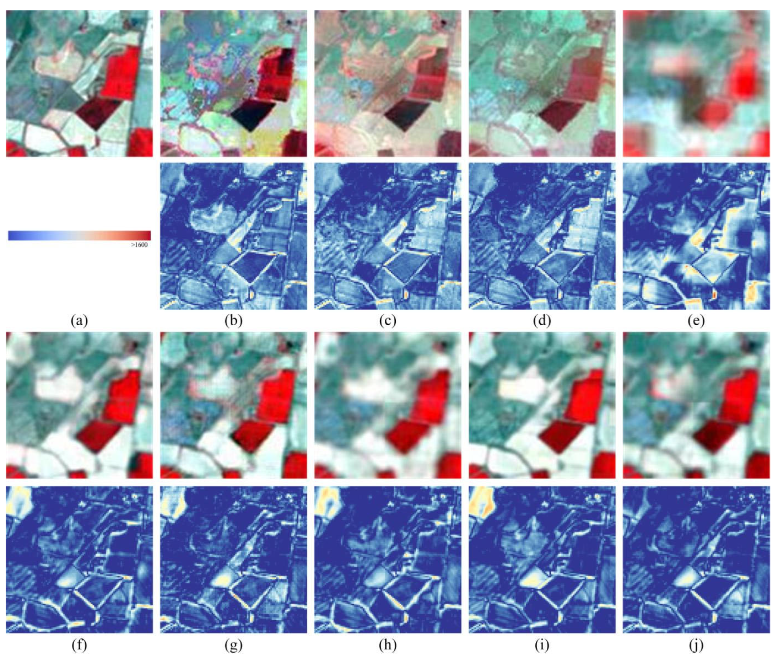
3.3. Experimental Results for CIA

For the CIA dataset, the input data consists of a MODIS–Landsat data pair from 25 November 2001 and MODIS data from 12 January 2002. During this period, significant tonal differences exist between images from different time points due to phenological changes. Figure 5 presents the prediction results for the Landsat data from 12 January 2002 using various STF methods. Figure 5a depicts the true image. While all methods capture phenological changes to some extent, a detailed analysis reveals noticeable color distortions in the irrigation areas in the results of STARFM, FSDAF, and Fit-FC. These distortions are likely due to the single-band computation approach employed by traditional methods. The EDCSTFN model, which emphasizes temporal changes, effectively captures phenological changes during the observation period. However, it struggles with structural reconstruction, leading to a loss of spatial details and resulting in a blurry appearance.
Figure 6 presents the predicted results for the zoomed-in subregion within the black box in Figure 5a, along with the AAD map comparing them to the true data. It is observed that STARFM and FSDAF exhibit significant color spots, while the EDCSTFN results display excessively blurred boundaries, exceeding the acceptable range. In contrast, other DL-based methods provide more natural color representation but still exhibit some issues. For example, MLFF-GAN, which focuses on temporal changes, introduces unpleasant noise in its results. STF-Trans, which emphasizes spatial detail enhancement, has lower clarity, likely due to its global feature extraction approach neglecting local high-frequency information. CTSTFM demonstrates notable errors in capturing phenological changes in the upper-left corner. The AAD map indicates that the proposed method achieves the smallest error, highlighting its superior performance in the phenological change prediction task.
Table 1 lists the RMSE, SSIM, UIQI, CC, ERGAS, and SAM evaluation metrics for each method on the CIA dataset, with the best values highlighted in bold. The results demonstrate that the proposed method outperforms others across all metrics, showing significant advantages in radiometric accuracy, structural restoration, and spectral fidelity.

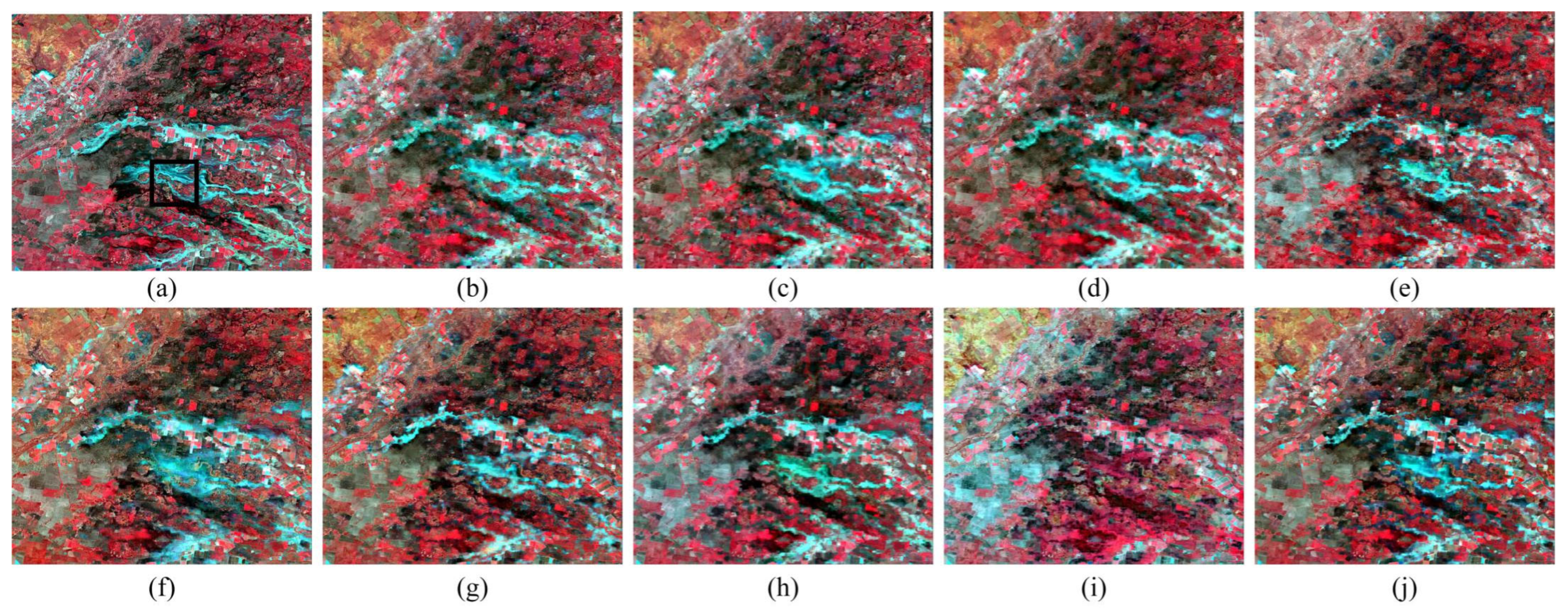
3.4. Experimental Results for LGC

For the LGC dataset, the input data includes MODIS–Landsat data pairs from 26 November 2004 and MODIS data from 12 December 2004. Significant differences exist between the two temporal scenes due to the impact of flooding. Compared to the prediction of phenological changes, predicting sudden land cover changes is more challenging. Figure 7 shows the predicted results for the LGC data on 12 December 2004 using different methods. Overall, except for CTSTFM, all other methods made relatively accurate predictions of the flood-affected areas. However, due to the significant spatial resolution difference between MODIS and Landsat, and the reliance on MODIS imagery at the prediction time for spatial information on the changes, the details of the flood-affected areas could not be perfectly restored. A zoomed-in view of the black-boxed region from the true Landsat image in Figure 7a is taken, and the AAD map for that region is calculated, as shown in Figure 8. It can be observed that the advantages of DL methods on the LGC dataset are not as pronounced as those on the CIA dataset. From the AAD results, FSDAF, despite being a traditional method based on simple theories, demonstrates relatively good fusion performance due to its consideration of both class changes and spatial reconstruction. In contrast, CTSTFM, which emphasizes spatial detail enhancement, fails to capture temporal changes, resulting in significant errors in the flood-affected areas. The proposed method continues to demonstrate the smallest error values.
Table 2 summarizes the performance metrics for each method applied to the LGC dataset, with the best values highlighted in bold. The results clearly demonstrate that the proposed method achieves optimal performance across most metrics. Notably, in the last three bands, the proposed method significantly outperforms the others, indicating its superior performance even in scenarios involving substantial changes.

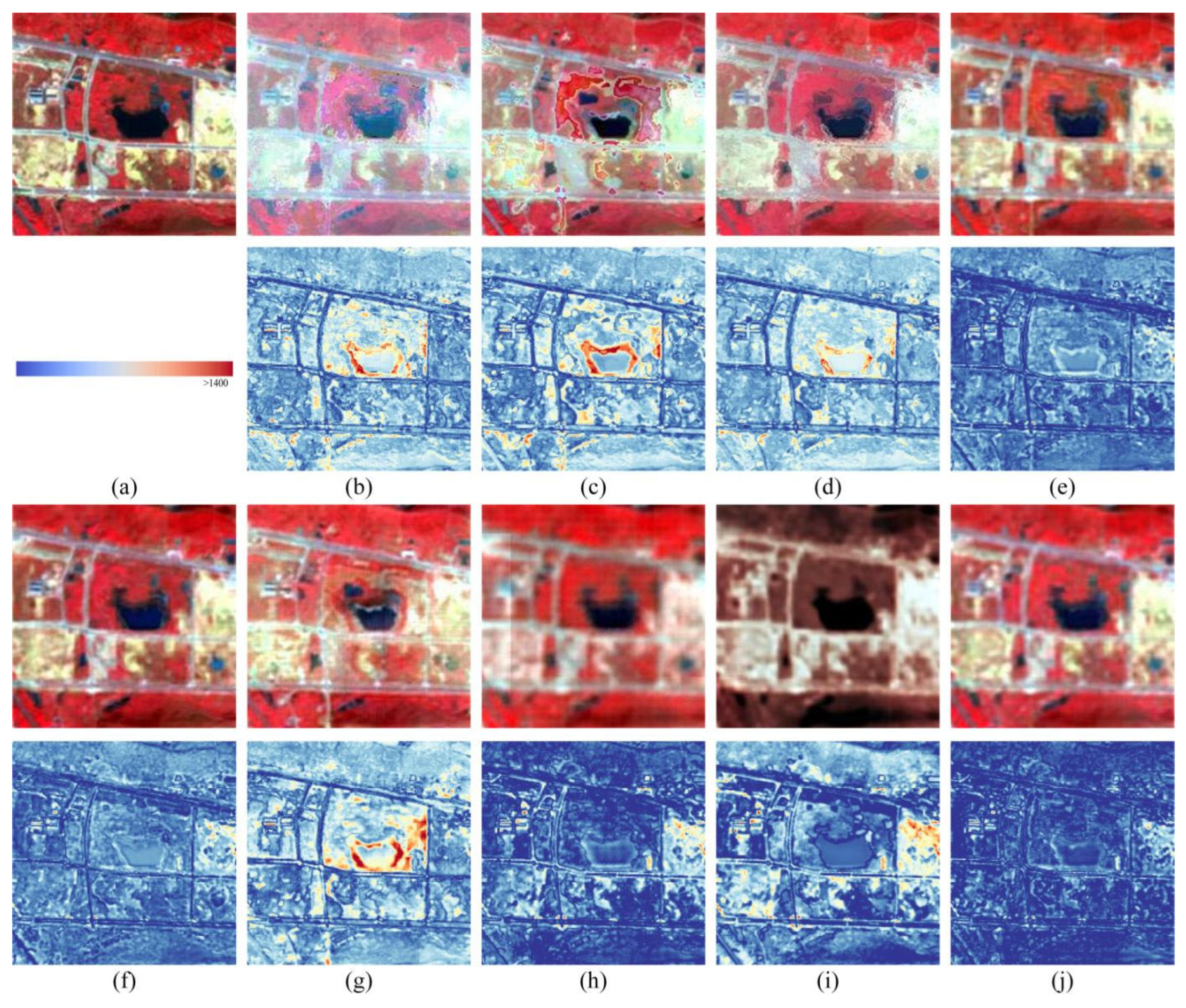
3.5. Experimental Results for Wuhan

Compared to the CIA and LGC datasets, the Wuhan dataset exhibits three distinct characteristics: first, it covers an urban area with more complex land cover textures; second, it comprises Landsat–GF images rather than the traditional MODIS–Landsat pairs; and third, the dataset is relatively small in scale. In this study, 30 October 2017 is selected as the reference time and 18 October 2015 as the prediction time. Figure 9 shows the global fusion results of different STF models on the Wuhan dataset. Compared to Figure 9a, the results of CTSTFM, which focuses on spatial detail reconstruction, exhibit noticeable color errors relative to the true image. According to Table 3, this issue likely stems from poor prediction in the near-infrared band, indicating insufficient learning of near-infrared features by the model. FSDAF shows noticeable artifacts in the densely built-up areas near the center of the image. For the water region at the top of the result image, MLFF-GAN, STF-Trans, and CTSTFM all display visible stitching marks. Special attention is given to the water area marked by the black box in Figure 9a, where significant changes occurred during the study period. Compared to 18 October 2015, the water area decreased by 30 October 2017. The zoomed-in view and corresponding error map are shown in Figure 10. The AAD map reveals that the three traditional methods and the temporal change-focused MLFF-GAN failed to capture this change effectively. In contrast, the proposed method is more sensitive to changes in the water boundary than the spatial detail enhancement-focused STF-Trans and CTSTFM. Furthermore, it demonstrates superior overall detail reconstruction compared to the temporal change-focused EDCSTFN.
Table 3 presents a quantitative comparison of fusion results on the Wuhan dataset. EDCSTFN achieves the highest CC metric; however, its performance on other metrics is less competitive, indicating that although EDCSTFN-generated images align well with the overall trends of the real images, they contain relatively large local errors. In contrast, the proposed method attains the second-highest CC value and outperforms all other methods on the remaining metrics.

4. Discussion

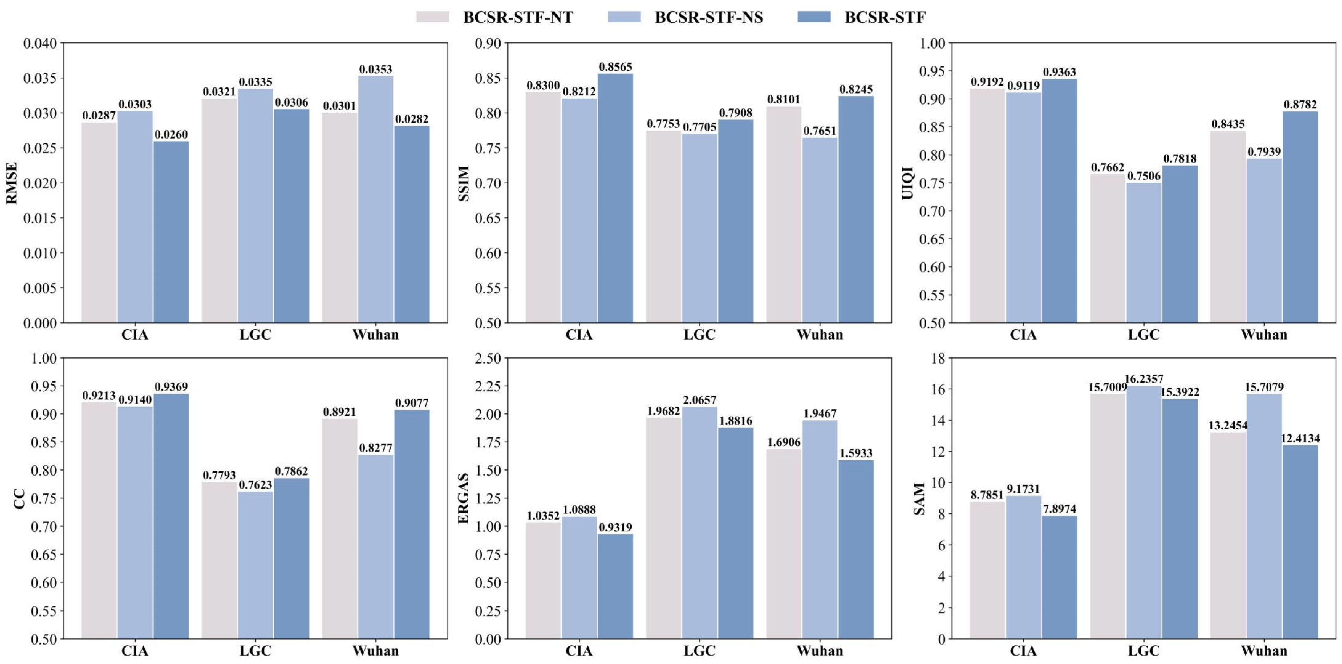
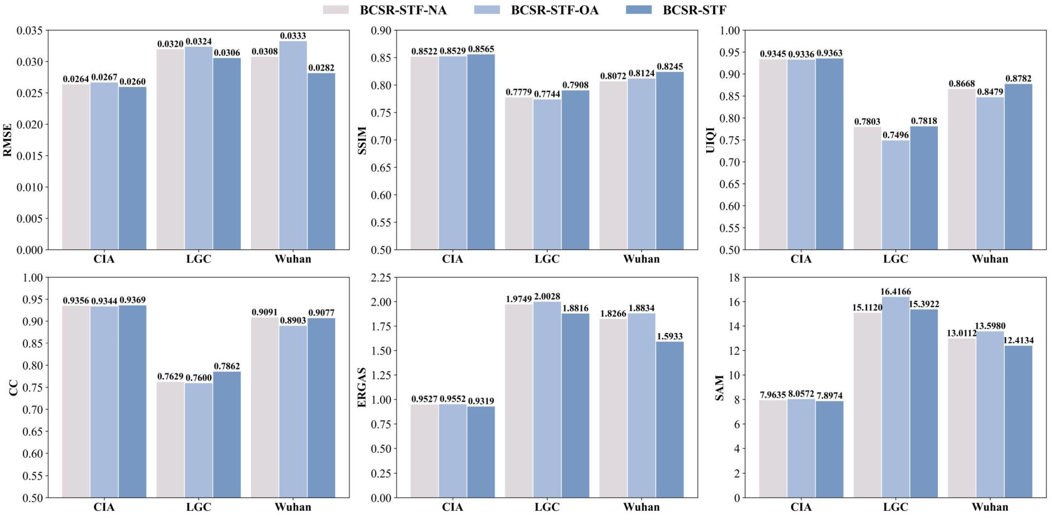
4.1. Ablation Studies

In this section, we perform ablation studies on the CIA, LGC, and Wuhan datasets.

4.1.1. Progressive Spatiotemporal Feature Fusion and Restoration

In the proposed BCSR-STF, the multi-layer PSTFR module serves as the core component, designed to perform iterative processing across multiple scales. To evaluate the effectiveness of this multi-layer structure, a single-layer variant named BCSR-STF-S is introduced for an ablation study. In BCSR-STF-S, feature extraction is applied only once to the input images from both the reference and prediction times, while all other settings remain unchanged. The results, presented in Figure 11, demonstrate that BCSR-STF consistently outperforms BCSR-STF-S. This improvement is attributed to the multi-layer design, which provides greater adaptability and better addresses challenges arising from varying image resolutions and temporal differences. At coarser scales, the model captures global information using lower-resolution features, whereas at finer scales, it restores high-resolution details and enhances spatiotemporal features, thereby mitigating the risk of information loss.

4.1.2. Bidirectional Cross Fusion

The BCF module significantly enhances spatiotemporal fusion by simultaneously addressing both the time and scale directions. To evaluate the effectiveness of this Bidirectional Cross Fusion module, two ablation experiments were conducted by removing the fusion modules for the temporal and scale directions. Specifically, the model without temporal fusion was designated BCSR-STF-NT (No Time direction), and the model without scale fusion was designated BCSR-STF-NS (No Scale direction).
For BCSR-STF-NT, we removed the cross-temporal feature fusion in the time direction and only performed spatiotemporal fusion in the scale direction, with other settings unchanged. Similarly, BCSR-STF-NS removed the cross-scale feature fusion in the scale direction and only performed spatiotemporal fusion in the time direction. The results of the ablation experiments, shown in Figure 12, demonstrate that BCSR-STF outperforms both BCSR-STF-NT and BCSR-STF-NS. This improvement can be attributed to the design of the Bidirectional Cross Fusion module. The fusion in the time direction helps capture temporal variation features, while the fusion in the scale direction enhances the detailed information between different resolutions. By simultaneously utilizing both directions of fusion, BCSR-STF can better handle spatiotemporal differences, providing more comprehensive and detailed spatiotemporal features.

4.1.3. Global Spectral Restoration and Feature Enhancement

The GSRFE module significantly enhances spatiotemporal fusion by adaptively adjusting spectral features. To validate the effectiveness of the GSRFE module, we designed two ablation experiments: one without spectral adjustment and one with only spectral adjustment but no feature enhancement. Specifically, we named the model without spectral adjustment as BCSR-STF-NA (No Spectral Adjustment) and the model with only spectral adjustment but no feature enhancement as BCSR-STF-OA (Only Spectral Adjustment). In BCSR-STF-NA, we removed the GSRFE module and directly used the spatiotemporal fusion result F s t ( i ) as the output. For BCSR-STF-OA, we only used the result F s t ( i ) that had undergone spectral adaptive adjustment without any feature enhancement. Other settings remained unchanged.
The results of the ablation experiments, shown in Figure 13, indicate that BCSR-STF outperforms both BCSR-STF-NA and BCSR-STF-OA. This improvement can be attributed to the combination of spectral adaptive adjustment and feature enhancement in the GSRFE module. The spectral adaptive adjustment helps correct spectral inconsistencies caused by sensor errors, while feature enhancement further improves the expressive capability of the spatiotemporal fusion features.

4.2. Computation Load

In this study, FLOPs (Floating-Point Operations per Second) and the number of parameters are used to measure the computational cost of the models. FLOPs represent the total number of floating-point operations required during the inference process and serve as a key metric for evaluating computational complexity. The input data size is set to (1, 6, 256, 256), where 1 denotes the batch size, 6 represents the number of input channels, and 256 × 256 corresponds to the resolution of the input image. By calculating FLOPs and the number of parameters, the computational efficiency and resource requirements of the models are comprehensively assessed. The results are presented in Table 4.
As shown in Table 4, although the parameter count of BCSR-STF reaches 34.80 M, which is higher than that of other lightweight models, its FLOPs are only 2.71 × 10¹⁰, significantly lower than the self-attention-based models STF-Trans and CTSTFM. This advantage is primarily attributed to its pyramid structure and windowed attention mechanism, which strike a well-balanced trade-off between computational efficiency and model performance. Furthermore, the results from three experimental datasets demonstrate that BCSR-STF exhibits the best robustness, effectively adapting to diverse scenarios and varying data distributions. For dense prediction tasks such as image fusion, a moderate increase in parameter count is generally accepted in exchange for improved model expressiveness and performance.

5. Conclusions

This work proposes BCSR-STF, a model designed to generate time series remote sensing data via spatiotemporal fusion. BCSR-STF integrates a multi-layer PSTFR structure, enabling iterative optimization of spatiotemporal features across multiple scales and enhancing adaptability to variations in resolution and temporal differences. The core components of PSTFR are the Bidirectional Cross Fusion (BCF) and Global Spectral Restoration and Feature Enhancement (GSRFE) modules. BCF significantly improves the fusion of spatiotemporal features by simultaneously processing information along both temporal and scale dimensions. GSRFE effectively corrects sensor errors and spectral inconsistencies through adaptive spectral adjustment and feature enhancement. The effectiveness of each module is validated through a series of ablation experiments. Comparative studies demonstrate the superior performance of BCSR-STF. However, the model demands substantial computational resources, potentially limiting its applicability in resource-constrained environments. Future work will focus on reducing computational complexity and resource consumption through algorithmic optimizations, such as model pruning and quantization, as well as the design of lightweight network architectures.

Author Contributions

Conceptualization, D.Z. and K.W.; methodology, D.Z.; Writing—original draft, D.Z.; writing—review and editing, K.W. and G.X. All authors have read and agreed to the published version of the manuscript.

Funding

This work was supported by the National Natural Science Foundation of China, grant number U21A2013; the Open Fund of Key Laboratory of Space Ocean Remote Sensing and Application, MNR, grant number 202401001; the Fundamental Research Funds for the Central Universities, China University of Geosciences (Wuhan), grant number 2642022009; the Open Fund of Wenzhou Future City Research Institute, grant number WL2023007; the Zhejiang Provincial Philosophy and Social Sciences Planning Project grant number 25NDJC096YBM; the Major Science and Technology Research Projects in Wenzhou City in 2023, grant number ZZN2023005; the Global Change and Air-Sea Interaction II, grant number GASI-01-DLYG-WIND0; the Foundation of State Key Laboratory of Public Big Data, grant number PBD2023-28; the Open Fund of Key Laboratory of Regional Development and Environmental Response, grant number 2023(A)003; and the Open Fund of State Key Laboratory of Remote Sensing Science, grant number OFSLRSS202312.

Institutional Review Board Statement

Not applicable.

Informed Consent Statement

Not applicable.

Data Availability Statement

The data presented in this study were derived from the following resources available in the public domain: CIA, https://data.csiro.au/collections/collection/CIcsiro%3A5846v3, accessed on 1 May 2025; LGC, https://data.csiro.au/collections/collection/CIcsiro:5847v003, accessed on 1 May 2025; Wuhan, https://github.com/lixinghua5540/Wuhan-dataset, accessed on 1 May 2025.

Acknowledgments

The authors express their gratitude to the scholars that produced and shared the codes of STARFM, FSDAF, Fit-FC, EDCSTFN, GAN-STFM, and MLFF-GAN models. The authors would like to thank the editors and anonymous reviewers for their insightful comments and suggestions that lead to this improved version and clearer presentation of the technical content.

Conflicts of Interest

The authors declare no conflicts of interest.

Abbreviations

The following abbreviations are used in this manuscript:
STFSpatiotemporal fusion
DLDeep learning
CNNConvolutional neural network
GANGenerative adversarial network
SRSuper-resolution
NDVINormalized difference vegetation index
PSTFRProgressive Spatiotemporal Feature Fusion and Restoration
BCFBidirectional Cross Fusion
GSRFEGlobal Spectral Restoration and Feature Enhancement
AdaINAdaptive Instance Normalization
SDAShort-distance attention
LDALong-distance attention
MLPMulti-layer perceptron
CIAColeambally Irrigation Area
LGCLower Gwydir Catchment
RMSERoot Mean Square Error
SSIMStructure Similarity Index
UIQIUniversal Image Quality Index
CCCorrelation Coefficient
SAMSpectral Angle Mapper
ERGASErreur Relative Global Adimensionnelle de Synthène
AADAverage Absolute Difference
FLOPsFloating Point Operations per Second

References

  1. Zhu, X.; Cai, F.; Tian, J.; Williams, T. Spatiotemporal Fusion of Multisource Remote Sensing Data: Literature Survey, Taxonomy, Principles, Applications, and Future Directions. Remote Sens. 2018, 10, 527. [Google Scholar] [CrossRef]
  2. Li, J.; Hong, D.; Gao, L.; Yao, J.; Zheng, K.; Zhang, B.; Chanussot, J. Deep Learning in Multimodal Remote Sensing Data Fusion: A Comprehensive Review. Int. J. Appl. Earth Obs. Geoinf. 2022, 112, 102926. [Google Scholar] [CrossRef]
  3. Wang, Z.; Ma, Y.; Zhang, Y. Review of Pixel-Level Remote Sensing Image Fusion Based on Deep Learning. Inf. Fusion 2023, 90, 36–58. [Google Scholar] [CrossRef]
  4. Mbabazi, D.; Mohanty, B.P.; Gaur, N. High Spatio-Temporal Resolution Evapotranspiration Estimates within Large Agricultural Fields by Fusing Eddy Covariance and Landsat Based Data. Agric. For. Meteorol. 2023, 333, 109417. [Google Scholar] [CrossRef]
  5. Ferreira, T.R.; Maguire, M.S.; da Silva, B.B.; Neale, C.M.U.; Serrão, E.A.O.; Ferreira, J.D.; de Moura, M.S.B.; dos Santos, C.A.C.; Silva, M.T.; Rodrigues, L.N.; et al. Assessment of Water Demands for Irrigation Using Energy Balance and Satellite Data Fusion Models in Cloud Computing: A Study in the Brazilian Semiarid Region. Agric. Water Manag. 2023, 281, 108260. [Google Scholar] [CrossRef]
  6. Bilotta, G.; Genovese, E.; Citroni, R.; Cotroneo, F.; Meduri, G.M.; Barrile, V. Integration of an Innovative Atmospheric Forecasting Simulator and Remote Sensing Data into a Geographical Information System in the Frame of Agriculture 4.0 Concept. AgriEngineering 2023, 5, 1280–1301. [Google Scholar] [CrossRef]
  7. Zhou, Y.; Liu, T.; Batelaan, O.; Duan, L.; Wang, Y.; Li, X.; Li, M. Spatiotemporal Fusion of Multi-Source Remote Sensing Data for Estimating Aboveground Biomass of Grassland. Ecol. Indic. 2023, 146, 109892. [Google Scholar] [CrossRef]
  8. Shi, C.; Wang, N.; Zhang, Q.; Liu, Z.; Zhu, X. A Comprehensive Flexible Spatiotemporal DAta Fusion Method (CFSDAF) for Generating High Spatiotemporal Resolution Land Surface Temperature in Urban Area. IEEE J. Sel. Top. Appl. Earth Obs. Remote Sens. 2022, 15, 9885–9899. [Google Scholar] [CrossRef]
  9. Pan, L.; Lu, L.; Fu, P.; Nitivattananon, V.; Guo, H.; Li, Q. Understanding Spatiotemporal Evolution of the Surface Urban Heat Island in the Bangkok Metropolitan Region from 2000 to 2020 Using Enhanced Land Surface Temperature. Geomat. Nat. Hazards Risk 2023, 14, 2174904. [Google Scholar] [CrossRef]
  10. Zhukov, B.; Oertel, D.; Lanzl, F.; Reinhackel, G. Unmixing-Based Multisensor Multiresolution Image Fusion. IEEE Trans. Geosci. Remote Sens. 1999, 37, 1212–1226. [Google Scholar] [CrossRef]
  11. Zhu, X.; Helmer, E.H.; Gao, F.; Liu, D.; Chen, J.; Lefsky, M.A. A Flexible Spatiotemporal Method for Fusing Satellite Images with Different Resolutions. Remote Sens. Environ. 2016, 172, 165–177. [Google Scholar] [CrossRef]
  12. Liu, W.; Zeng, Y.; Li, S.; Huang, W. Spectral Unmixing Based Spatiotemporal Downscaling Fusion Approach. Int. J. Appl. Earth Obs. Geoinf. 2020, 88, 102054. [Google Scholar] [CrossRef]
  13. Gao, F.; Masek, J.; Schwaller, M.; Hall, F. On the Blending of the Landsat and MODIS Surface Reflectance: Predicting Daily Landsat Surface Reflectance. IEEE Trans. Geosci. Remote Sens. 2006, 44, 2207–2218. [Google Scholar] [CrossRef]
  14. Zhu, X.; Chen, J.; Gao, F.; Chen, X.; Masek, J.G. An Enhanced Spatial and Temporal Adaptive Reflectance Fusion Model for Complex Heterogeneous Regions. Remote Sens. Environ. 2010, 114, 2610–2623. [Google Scholar] [CrossRef]
  15. Wang, Q.; Atkinson, P.M. Spatio-Temporal Fusion for Daily Sentinel-2 Images. Remote Sens. Environ. 2018, 204, 31–42. [Google Scholar] [CrossRef]
  16. Li, A.; Bo, Y.; Zhu, Y.; Guo, P.; Bi, J.; He, Y. Blending Multi-Resolution Satellite Sea Surface Temperature (SST) Products Using Bayesian Maximum Entropy Method. Remote Sens. Environ. 2013, 135, 52–63. [Google Scholar] [CrossRef]
  17. Liao, L.; Song, J.; Wang, J.; Xiao, Z.; Wang, J. Bayesian Method for Building Frequent Landsat-Like NDVI Datasets by Integrating MODIS and Landsat NDVI. Remote Sens. 2016, 8, 452. [Google Scholar] [CrossRef]
  18. Huang, B.; Song, H. Spatiotemporal Reflectance Fusion via Sparse Representation. IEEE Trans. Geosci. Remote Sens. 2012, 50, 3707–3716. [Google Scholar] [CrossRef]
  19. Song, H.; Huang, B. Spatiotemporal Satellite Image Fusion Through One-Pair Image Learning. IEEE Trans. Geosci. Remote Sens. 2013, 51, 1883–1896. [Google Scholar] [CrossRef]
  20. Tan, Z.; Yue, P.; Di, L.; Tang, J. Deriving High Spatiotemporal Remote Sensing Images Using Deep Convolutional Network. Remote Sens. 2018, 10, 1066. [Google Scholar] [CrossRef]
  21. Tan, Z.; Di, L.; Zhang, M.; Guo, L.; Gao, M. An Enhanced Deep Convolutional Model for Spatiotemporal Image Fusion. Remote Sens. 2019, 11, 2898. [Google Scholar] [CrossRef]
  22. Tan, Z.; Gao, M.; Li, X.; Jiang, L. A Flexible Reference-Insensitive Spatiotemporal Fusion Model for Remote Sensing Images Using Conditional Generative Adversarial Network. IEEE Trans. Geosci. Remote Sens. 2022, 60, 5601413. [Google Scholar] [CrossRef]
  23. Song, B.; Liu, P.; Li, J.; Wang, L.; Zhang, L.; He, G.; Chen, L.; Liu, J. MLFF-GAN: A Multilevel Feature Fusion with GAN for Spatiotemporal Remote Sensing Images. IEEE Trans. Geosci. Remote Sens. 2022, 60, 4410816. [Google Scholar] [CrossRef]
  24. Vaswani, A.; Shazeer, N.; Parmar, N.; Uszkoreit, J.; Jones, L.; Gomez, A.N.; Kaiser, L.; Polosukhin, I. Attention Is All You Need 2017. Adv. Neural Inf. Process. Syst. 2017, 30. [Google Scholar]
  25. Dosovitskiy, A.; Beyer, L.; Kolesnikov, A.; Weissenborn, D.; Zhai, X.; Unterthiner, T.; Dehghani, M.; Minderer, M.; Heigold, G.; Gelly, S.; et al. An Image Is Worth 16 × 16 Words: Transformers for Image Recognition at Scale. arXiv 2021, arXiv:2010.11929. [Google Scholar]
  26. Chen, G.; Jiao, P.; Hu, Q.; Xiao, L.; Ye, Z. SwinSTFM: Remote Sensing Spatiotemporal Fusion Using Swin Transformer. IEEE Trans. Geosci. Remote Sens. 2022, 60, 5410618. [Google Scholar] [CrossRef]
  27. Liu, Z.; Lin, Y.; Cao, Y.; Hu, H.; Wei, Y.; Zhang, Z.; Lin, S.; Guo, B. Swin Transformer: Hierarchical Vision Transformer Using Shifted Windows. In Proceedings of the 2021 IEEE/CVF International Conference on Computer Vision (ICCV 2021), Montreal, BC, Canada, 11–17 October 2021; IEEE: New York, NY, USA, 2021; pp. 9992–10002. [Google Scholar]
  28. Benzenati, T.; Kallel, A.; Kessentini, Y. STF-Trans: A Two-Stream Spatiotemporal Fusion Transformer for Very High Resolution Satellites Images. Neurocomputing 2024, 563, 126868. [Google Scholar] [CrossRef]
  29. Jiang, M.; Shao, H. A CNN-Transformer Combined Remote Sensing Imagery Spatiotemporal Fusion Model. IEEE J. Sel. Top. Appl. Earth Obs. Remote Sens. 2024, 17, 13995–14009. [Google Scholar] [CrossRef]
  30. Liu, X.; Deng, C.; Chanussot, J.; Hong, D.; Zhao, B. StfNet: A Two-Stream Convolutional Neural Network for Spatiotemporal Image Fusion. IEEE Trans. Geosci. Remote Sens. 2019, 57, 6552–6564. [Google Scholar] [CrossRef]
  31. Li, W.; Yang, C.; Peng, Y.; Du, J. A Pseudo-Siamese Deep Convolutional Neural Network for Spatiotemporal Satellite Image Fusion. IEEE J. Sel. Top. Appl. Earth Obs. Remote Sens. 2022, 15, 1205–1220. [Google Scholar] [CrossRef]
  32. Chen, Y.; Shi, K.; Ge, Y.; Zhou, Y. Spatiotemporal Remote Sensing Image Fusion Using Multiscale Two-Stream Convolutional Neural Networks. IEEE Trans. Geosci. Remote Sens. 2022, 60, 1–12. [Google Scholar] [CrossRef]
  33. Li, W.; Zhang, X.; Peng, Y.; Dong, M. DMNet: A Network Architecture Using Dilated Convolution and Multiscale Mechanisms for Spatiotemporal Fusion of Remote Sensing Images. IEEE Sens. J. 2020, 20, 12190–12202. [Google Scholar] [CrossRef]
  34. Li, W.; Zhang, X.; Peng, Y.; Dong, M. Spatiotemporal Fusion of Remote Sensing Images Using a Convolutional Neural Network with Attention and Multiscale Mechanisms. Int. J. Remote Sens. 2021, 42, 1973–1993. [Google Scholar] [CrossRef]
  35. Zhang, Y.; Liu, J.; Liang, S.; Li, M. A New Spatial–Temporal Depthwise Separable Convolutional Fusion Network for Generating Landsat 8-Day Surface Reflectance Time Series over Forest Regions. Remote Sens. 2022, 14, 2199. [Google Scholar] [CrossRef]
  36. Liu, Q.; Meng, X.; Shao, F.; Li, S. PSTAF-GAN: Progressive Spatio-Temporal Attention Fusion Method Based on Generative Adversarial Network. IEEE Trans. Geosci. Remote Sens. 2022, 60, 5408513. [Google Scholar] [CrossRef]
  37. Song, H.; Liu, Q.; Wang, G.; Hang, R.; Huang, B. Spatiotemporal Satellite Image Fusion Using Deep Convolutional Neural Networks. IEEE J. Sel. Top. Appl. Earth Obs. Remote Sens. 2018, 11, 821–829. [Google Scholar] [CrossRef]
  38. Liu, H.; Yang, G.; Deng, F.; Qian, Y.; Fan, Y. MCBAM-GAN: The Gan Spatiotemporal Fusion Model Based on Multiscale and CBAM for Remote Sensing Images. Remote Sens. 2023, 15, 1583. [Google Scholar] [CrossRef]
  39. Jia, D.; Song, C.; Cheng, C.; Shen, S.; Ning, L.; Hui, C. A Novel Deep Learning-Based Spatiotemporal Fusion Method for Combining Satellite Images with Different Resolutions Using a Two-Stream Convolutional Neural Network. Remote Sens. 2020, 12, 698. [Google Scholar] [CrossRef]
  40. Jia, D.; Cheng, C.; Shen, S.; Ning, L. Multitask Deep Learning Framework for Spatiotemporal Fusion of NDVI. IEEE Trans. Geosci. Remote Sens. 2022, 60, 5616313. [Google Scholar] [CrossRef]
  41. Wang, W.; Chen, W.; Qiu, Q.; Chen, L.; Wu, B.; Lin, B.; He, X.; Liu, W. CrossFormer++: A Versatile Vision Transformer Hinging on Cross-Scale Attention. IEEE Trans. Pattern Anal. Mach. Intell. 2024, 46, 3123–3136. [Google Scholar] [CrossRef]
  42. Emelyanova, I.V.; McVicar, T.R.; Van Niel, T.G.; Li, L.T.; Van Dijk, A.I.J.M. Assessing the Accuracy of Blending Landsat–MODIS Surface Reflectances in Two Landscapes with Contrasting Spatial and Temporal Dynamics: A Framework for Algorithm Selection. Remote Sens. Environ. 2013, 133, 193–209. [Google Scholar] [CrossRef]
  43. Zhang, X.; Xie, L.; Li, S.; Lei, F.; Cao, L.; Li, X. Wuhan Dataset: A High-Resolution Dataset of Spatiotemporal Fusion for Remote Sensing Images. IEEE Geosci. Remote Sens. Lett. 2024, 21, 2504305. [Google Scholar] [CrossRef]
Figure 1. Overall model structure of the proposed BCSR-STF.
Applsci 15 06649 g001
Figure 2. Bidirectional Cross Fusion module.
Applsci 15 06649 g002
Figure 3. The pixel grouping methods in (a) SDA and (b) LDA.
Applsci 15 06649 g003
Figure 4. Global Spectral Restoration and Feature Enhancement.
Applsci 15 06649 g004
Figure 5. Fusion results on 12 January 2001, generated by different models on the CIA dataset. (a) Ground truth. (b) STARFM. (c) FSDAF. (d) Fit-FC. (e) EDCSTFN. (f) GAN-STFM. (g) MLFF-GAN. (h) STF-Trans. (i) CTSTFM. (j) Proposed.
Applsci 15 06649 g005
Figure 6. Fusion and AAD visualizations for the subregions on 12 January 2001, generated by different models on the CIA dataset. (a) Ground truth. (b) STARFM. (c) FSDAF. (d) Fit-FC. (e) EDCSTFN. (f) GAN-STFM. (g) MLFF-GAN. (h) STF-Trans. (i) CTSTFM. (j) Proposed.
Applsci 15 06649 g006
Figure 7. Fusion results on 12 December 2004, generated by different models on the LGC dataset. (a) Ground truth. (b) STARFM. (c) FSDAF. (d) Fit-FC. (e) EDCSTFN. (f) GAN-STFM. (g) MLFF-GAN. (h) STF-Trans. (i) CTSTFM. (j) Proposed.
Applsci 15 06649 g007
Figure 8. Fusion and AAD visualizations for subregions on 12 December 2004. for the subregions on 12 December 2004, generated by different models on the LGC dataset. (a) Ground truth. (b) STARFM. (c) FSDAF. (d) Fit-FC. (e) EDCSTFN. (f) GAN-STFM. (g) MLFF-GAN. (h) STF-Trans. (i) CTSTFM. (j) Proposed.
Applsci 15 06649 g008
Figure 9. Fusion results on 18 October 2015, generated by different models on the Wuhan dataset. (a) Ground truth. (b) STARFM. (c) FSDAF. (d) Fit-FC. (e) EDCSTFN. (f) GAN-STFM. (g) MLFF-GAN. (h) STF-Trans. (i) CTSTFM. (j) Proposed.
Applsci 15 06649 g009
Figure 10. Fusion results and error maps for the subregions on 18 October 2015, generated by different models on the Wuhan dataset. (a) Ground truth. (b) STARFM. (c) FSDAF. (d) Fit-FC. (e) EDCSTFN. (f) GAN-STFM. (g) MLFF-GAN. (h) STF-Trans. (i) CTSTFM. (j) Proposed.
Applsci 15 06649 g010
Figure 11. Quantitative evaluation results of BCSR-STF and BCSR-STF-S.
Applsci 15 06649 g011
Figure 12. Quantitative evaluation results of BCSR-STF, BCSR-STF-NT, and BCSR-STF-NS.
Applsci 15 06649 g012
Figure 13. Quantitative evaluation results of BCSR-STF, BCSR-STF-NA, and BCSR-STF-OA.
Applsci 15 06649 g013
Table 1. Quantitative evaluation results with different methods on the CIA dataset.
BandSTARFMFSDAFFit-FCEDCSTFNGAN-STFMMLFF-GANSTF-TransCTSTFMProposed
RMSE10.01660.01610.01570.01620.01260.01220.01230.01330.0118
20.02500.02340.02350.02550.01800.01800.01670.01730.0164
30.03990.03640.03760.04360.02930.02860.02670.02730.0261
40.04960.05090.04720.04450.04010.03950.03740.03710.0370
50.04600.04590.04680.04770.03960.03740.03620.03750.0348
60.03790.03840.03850.03980.03440.03340.03240.03160.0302
Avg0.03580.03520.03490.03620.02900.02820.02700.02730.0260
SSIM10.89280.90070.89390.88500.92500.92860.93060.92710.9359
20.84640.85940.85360.82590.89660.89560.90300.90260.9084
30.77390.79100.78730.71650.84130.84630.85110.85430.8594
40.68110.67400.67850.71470.76080.76870.77100.78350.7873
50.74290.74980.74620.73770.80060.80560.80960.80800.8160
60.77480.78000.77230.77490.81780.81930.82840.82650.8318
Avg0.78530.79250.78860.77580.84040.84400.84890.85030.8565
UIQI10.81400.82930.81900.81520.89790.91130.92010.91070.9245
20.81520.83870.82750.80230.91070.91450.92790.92250.9312
30.81650.84980.84000.78150.91320.91780.92940.92640.9336
40.82750.82620.83700.88060.89760.90430.91280.91780.9184
50.92220.92470.92240.91740.94440.94910.95510.95280.9576
60.92060.92150.91930.91740.93680.94080.94770.94750.9521
Avg0.85270.86500.86090.85240.91680.92300.93220.92960.9363
CC10.83200.83700.84010.83310.90220.91160.92300.91480.9265
20.83690.85010.84730.82340.91530.91600.92920.92470.9320
30.84540.86540.85510.80130.91650.91980.93060.92750.9345
40.83440.82810.84590.88130.89940.90490.91410.91870.9186
50.92220.92490.92380.91800.94510.94970.95540.95320.9577
60.92100.92170.91980.91770.93760.94120.94840.94780.9523
Avg0.86530.87120.87200.86250.91940.92390.93340.93110.9369
ERGASALL1.31461.26661.26121.34881.02981.00470.96400.99310.9319
SAMALL11.125610.910410.832611.47568.88988.66798.09708.24947.8974
The best values of the index are marked in bold.
Table 2. Quantitative evaluation results with different methods on the LGC dataset.
BandSTARFMFSDAFFit-FCEDCSTFNGAN-STFMMLFF-GANSTF-TransCTSTFMProposed
RMSE10.01430.01490.01400.01510.01460.01610.01420.01670.0143
20.02000.02070.02010.02000.02070.02230.02030.02340.0214
30.02510.02580.02510.02570.02640.02690.02600.03200.0256
40.03760.03970.03850.03940.0410.04000.03600.05320.0351
50.05680.06210.05650.05900.0540.05330.05740.06600.0503
60.04550.05150.04460.04070.03990.04040.04110.04760.0372
Avg0.03320.03580.03310.03330.03280.03320.03250.03980.0306
SSIM10.91320.91250.92330.92280.91850.90590.92170.91660.9268
20.87300.87090.88000.88970.88010.87090.88560.88430.8888
30.83500.83310.84380.84550.84130.83560.84980.83910.8562
40.72920.72940.74050.70830.70370.72390.74090.69100.7593
50.56970.52200.55320.55130.56960.59480.57970.57660.6241
60.64080.57540.62740.62670.64380.65330.64810.64730.6895
Avg0.76010.74050.76140.75740.75950.76410.77100.75910.7908
UIQI10.71520.70620.71240.61320.68440.68390.73130.58130.7354
20.70190.68900.69430.65600.68070.71250.72830.56370.7262
30.70720.69650.70070.65730.6960.71790.71840.53660.7541
40.78570.77940.78270.74310.7660.78260.81930.69910.8370
50.75310.71980.73130.66450.76590.79400.76630.74360.8169
60.72050.65310.70210.73160.77980.79180.78490.77130.8215
Avg0.73060.70730.72060.67760.72880.74710.75810.64930.7818
CC10.71580.70760.71600.65820.68780.68700.73220.60730.7363
20.70710.69160.70070.69580.68880.71690.72830.59020.7293
30.71300.70040.70860.68340.69940.71920.71880.54690.7564
40.80750.80110.80980.78320.7690.78710.83000.72430.8375
50.79090.76660.78320.76950.78640.79930.81090.77500.8282
60.78730.74730.77860.78710.78830.79770.81530.79490.8293
Avg0.75360.73580.74950.72950.73660.75120.77260.67310.7862
ERGASALL2.06552.22302.03222.02451.98372.03001.99382.38161.8816
SAMALL16.282617.029316.230316.817016.773816.557715.962018.040615.3922
The best values of the index are marked in bold.
Table 3. Quantitative evaluation results with different methods on the Wuhan dataset.
BandSTARFMFSDAFFit-FCEDCSTFNGAN-STFMMLFF-GANSTF-TransCTSTFMProposed
RMSE10.05830.05740.06360.03070.02570.04850.02240.02230.0195
20.04950.04780.05220.02940.03410.05350.02940.02880.0246
30.04590.04950.04370.03340.02790.05050.03630.03870.0274
40.05830.05990.05150.05070.06350.05680.05370.09700.0413
Avg0.05300.05360.05280.03610.03780.05230.03540.04670.0282
SSIM10.64480.63960.62390.80700.84330.69070.84050.86340.8820
20.66620.64370.66200.81280.80680.66440.78070.80930.8470
30.68380.61710.69110.80290.84970.65130.76040.79330.8483
40.55990.52140.58440.71720.71460.56340.60790.37770.7207
Avg0.63870.60540.64030.78500.80360.64240.74740.71090.8245
UIQI10.63750.59720.55360.76580.81590.61030.75990.72750.8579
20.70410.63360.64070.81330.81830.62680.76920.75620.8643
30.79690.71200.76900.84640.89650.70190.79940.78190.9106
40.77690.74050.78000.86000.84600.75860.80810.19070.8802
Avg0.72890.67080.68580.82140.84420.67440.78420.61410.8782
CC10.81060.78680.85190.91290.89450.77610.85720.82640.9013
20.79300.75990.85310.91390.89940.76450.86550.86110.9007
30.86360.78840.88450.93880.93250.78740.89260.87800.9235
40.81040.78100.84300.90770.90330.78630.78420.34000.8894
Avg0.81940.77900.85810.91830.90740.77860.86990.72640.9077
ERGASALL3.73443.70533.96522.17182.06953.47321.94072.16091.5933
SAMALL17.786919.363018.801214.518913.474419.371415.283517.185712.4134
The best values of the index are marked in bold.
Table 4. Model efficiency analysis of six deep learning-based spatiotemporal fusion models.
MODELParam. (M)FLOPs
EDCSTFN 0.281.86 × 1010
GAN-STFMGenerator0.583.78 × 1010
Discriminator3.671.03 × 107
MLFF-GANGenerator5.931.36 × 1010
Discriminator2.783.77 × 109
STF-Trans 23.341.74 × 1011
CTSTFM 6.303.8 × 1011
BCSR-STF 34.802.71 × 1010
Disclaimer/Publisher’s Note: The statements, opinions and data contained in all publications are solely those of the individual author(s) and contributor(s) and not of MDPI and/or the editor(s). MDPI and/or the editor(s) disclaim responsibility for any injury to people or property resulting from any ideas, methods, instructions or products referred to in the content.

