Improved Liquefaction Hazard Assessment via Deep Feature Extraction and Stacked Ensemble Learning on Microtremor Data

Abstract

The reduction in disaster risk in urban regions due to natural hazards (e.g., earthquakes, landslides, floods, and tropical cyclones) is primarily a development matter that must be treated within the scope of a broader urban development framework. Natural hazard assessment is one of the turning points in mitigating disaster risk, which typically contributes to stronger urban resilience and more sustainable urban development. Regarding this challenge, our research proposes a new approach in the signal processing chain and feature extraction from microtremor data that focuses mainly on the Horizontal-to-Vertical Spectral Ratio (HVSR) so as to assess liquefaction potential as a natural hazard using AI. The key raw seismic features of site amplification and resonance are extracted from the data via bandpass filtering, Fourier Transformation (FT), the calculation of the HVSR, and smoothing through the use of moving averages. The main novelty is the integration of machine learning, particularly stacked ensemble learning, for liquefaction potential classification from imbalanced seismic datasets. For this approach, several models are used to consider class imbalance, enhancing classification performance and offering better insight into liquefaction risk based on microtremor data. Then, the paper proposes a liquefaction detection method based on deep learning with an autoencoder and stacked classifiers. The autoencoder compresses data into the latent space, underlining the liquefaction features classified by the multi-layer perceptron (MLP) classifier and eXtreme Gradient Boosting (XGB) classifier, and the meta-model combines these outputs to put special emphasis on rare liquefaction events. This proposed methodology improved the detection of an imbalanced dataset, although challenges remain in both interpretability and computational complexity. We created a synthetic dataset of 1000 samples using realistic feature ranges that mimic the Rif data region to test model performance and conduct sensitivity analysis. Key seismic and geotechnical variables were included, confirming the amplification factor (Af) and seismic vulnerability index ($K_g$) as dominant predictors and supporting model generalizability in data-scarce regions. Our proposed method for liquefaction potential classification achieves 100% classification accuracy, 100% precision, and 100% recall, providing a new baseline. Compared to existing models such as XGB and MLP, the proposed model performs better in all metrics. This new approach could become a critical component in assessing liquefaction hazard, contributing to disaster mitigation and urban planning.

1. Introduction

Urban development serves as an integral part in minimizing natural hazards and strengthening emergency management in increasingly urbanizing regions. Integrating risk management frameworks into urban design promotes resilience and adaptation in the face of environmental challenges. However, governance difficulties, including institutional dispersion and unclear legal frameworks, can limit adequate hazard management strategies. Collaborative governance approaches that incorporate local communities, NGOs, and business sectors help overcome gaps in disaster preparation. By considering these challenges, cities can establish inclusive policies that preserve vulnerable populations and increase sustainability over the long term. efficient disaster risk management requires the combination of hazard assessment with urban design, ensuring facilities and resident populations stay safeguarded against unforeseen environmental hazards [1]. Among these hazards is soil liquefaction, a geotechnical phenomenon whereby saturated soils lose strength and take on a more liquid-like state when subjected to dynamic forces, as in the case of earthquakes. The increased pore water pressure within the shaking soil reduces the friction of the soil particles on each other, essentially making the soil behave as a liquid. This can leads to foundation failure or even complete structural collapse. A sudden loss of strength so great can lead to catastrophic results: liquefaction can collapse buildings, roads, and bridges [2,3,4,5]. Serious risk exists when loose, saturated soils are the base; that is why realistic predictions of locations likely to undergo liquefaction are critical components in disaster mitigation and urban planning with the aim of developing resilient infrastructure.

At places where this phenomenon may occur, earthquake-related destruction risks rise, mostly in areas exposed to danger, including the frontier territories of tectonic plates [6,7,8]. That is why realistic predictions of locations likely to undergo liquefaction are critical components in disaster mitigation and urban planning with the aim of developing resilient infrastructure.

The difficulty in identifying zones prone to liquefaction is due to the complexity of the physical properties of soils in different regions, including composition, grain size, density, and moisture content, which determine the overall behavior of the soil under seismic forces [9,10]. The factors that influence susceptibility to liquefaction include soil saturation, grain size distribution, and the seismic history of the area. These patterns are often subtle, complex, and nonlinear and require sophisticated models and techniques in data analysis to identify.

One of the most significant problems in developing reliable liquefaction prediction models is that liquefaction events are rare [11,12]. Seismic activity may be relatively low, or previous earthquakes may have not triggered liquefaction in a region. For this reason, datasets used in model training are usually hugely imbalanced, with an overwhelming proportion of data reflecting “normal” soil conditions that to not lead to liquefaction, even when subjected to seismic activity. This makes it difficult to use machine learning models, which tend to be biased toward the majority class and often fail to appropriately recognize the rare but critical instances of liquefaction.

So, to cope with this, advanced data-driven techniques that can distinguish areas prone to liquefaction from more stable soils due to complex patterns are required [13,14,15,16]. Traditional geophysical methods like geotechnical investigations and borehole tests are valuable but seriously limited in time, cost, and scalability. Most geotechnical investigations require the collection of field data at discrete locations, which is expensive and often not logistically feasible in large, remote, or inaccessible areas. The information obtained from the testing of boreholes is detailed but of a limited extent, and extending this information to a larger area is extremely resource-consuming.

Classic methods have been used to identify liquefaction, relying mainly on empirical correlations and probabilistic models such as Bayesian networks and Monte Carlo simulations based on geotechnical and seismic data. While powerful in developing the risk assessment process, these techniques were afflicted with assumptions about data distribution and how uncertainties are propagated [17].

Recent contributions to the subject include those of Kumar, Samui, & Burman, who designed a hybrid ANN optimized with metaheuristic techniques for the probabilistic prediction of liquefaction. They proved that the used of artificial neural networks combined with advanced optimization approaches led to a large boost in predictive accuracy relative to standard models [18]. Ghani et al. studied machine learning-based liquefaction prediction using seismic features with geotechnical datasets with hybrid models integrating SVM and RF, reaching an overall accuracy of 97%. The results reflect an ever-increasing contribution of machine learning in predictive reliability advancement [19]. Hu et al. developed continuous–discrete hybrid Bayesian network models and applied them to the the assessment of surface wave velocity (Vs) datasets for earthquake-induced liquefaction evaluation. This model was developed based on Bayesian inference methods that enhance the probabilistic evaluation, considering the uncertainty in soil and seismic properties discussed in [20].

Jas and Dodagoudar conducted a comprehensive analysis of machine learning applications in liquefaction research, outlining the evolution of hybrid machine learning methodologies from 1994 to 2021. Their analysis highlighted the necessity of integrating multiple ML algorithms into a single framework to enhance predictive robustness [21]. The most recent contributions were made by Kurnaz et al., who proposed an ANN model whose hyperparameters are optimized for liquefaction susceptibility prediction. Their works underlined how relevant hyperparameter tuning is in improving model accuracy when applied to seismic and soil datasets [22]. On the other hand, Hameed et al. explored the application of Extreme Learning Machines (ELMs) with dingo optimization algorithms and concluded that optimization-based hybrid models may enhance liquefaction prediction [23]. The role of ensemble learning frameworks was reinforced by [24]. Their study developed ensemble models that employed different ML methods to enhance the generalization and robustness of model performance predictions. Khatti et al. also presented a hybrid ML-based liquefaction assessment framework using cone penetration test data, which showed that deep learning combined with hybrid learning significantly improved the prediction accuracy for liquefaction-prone areas [25]. Probabilistic approaches still play a vital role in liquefaction risk assessment. Zhao et al. proposed a probabilistic energy-based machine learning model considering uncertainty quantification to improve reliability [26]. Ghani and Kumari. developed a hybrid computational framework using fuzzy logic and ML in liquefaction risk assessment [27]. From empirical and probabilistic models, the development of liquefaction identification methodologies has progressed to advanced machine learning and hybrid computational approaches, enhancing prediction capabilities considerably. However, these traditional methods have serious limitations.

Therefore, to cope with these challenges, the approach presented in this paper leverages a deep learning-based method [28] for liquefaction identification in the Rif region of Morocco. It has a key novelty by introducing an autoencoder that learns a compact 16D latent representation of input data. The proposed autoencoder model captures complex nonlinear relationships in liquefaction potential. By compressing the data into this latent space, the model decreases the dimensionality, retaining the most informative features and effectively abstracting the underlying patterns that indicate liquefaction risk.

Then, the autoencoder’s latent representations are fed through the stacked classifier model: an ensemble of two basic models’ outputs, an MLP classifier, and an XGB classifier. The MLP classifier represents a neural network-based model that can learn subtler nonlinear correlations among features. The XGB classifier is a gradient-boosted machine that has proven robust for dealing with imbalanced datasets. It provides the final prediction by intelligently incorporating, with the help of a meta-model, the outputs of several base classifiers, thereby allowing the model to pay a lot of attention to rare liquefaction events while overfitting for more typical soil conditions is kept in check.

This approach is particularly suited to the problems of the Rif region, where standard geophysical data could be sparse or uneven. Unlike relying solely on the extensive normal data, focusing on those rare abnormal events, this approach enhances liquefaction-prone location detection. By incorporating multiple learning algorithms, the model is more adaptable to various geographic conditions and could be applied to similar seismic zones, breaking the limits set by earlier models.

Initial tests of the proposed model in the Rif region were promising. The autoencoder learned intricate patterns within geophysical features that are not easily interpretable using the more standard analysis techniques. The stacked classifier, especially when combined with an MLP classifier [29] and XGB classifier [30], enhances this model’s power in identifying liquefaction events from this imbalanced dataset by achieving better classification accuracy and a reduction in the number of false negatives.

Despite the satisfactory performance of the model for the Rif-area dataset, its generalization capacity needs to be evaluated against other locations exhibiting seismic events under varying geological circumstances. More validation with diverse types of datasets will add strength to this model and adaptability to different approaches for liquefaction identification in varying geophysical contexts.

The key contributions of this paper are outlined as follows:

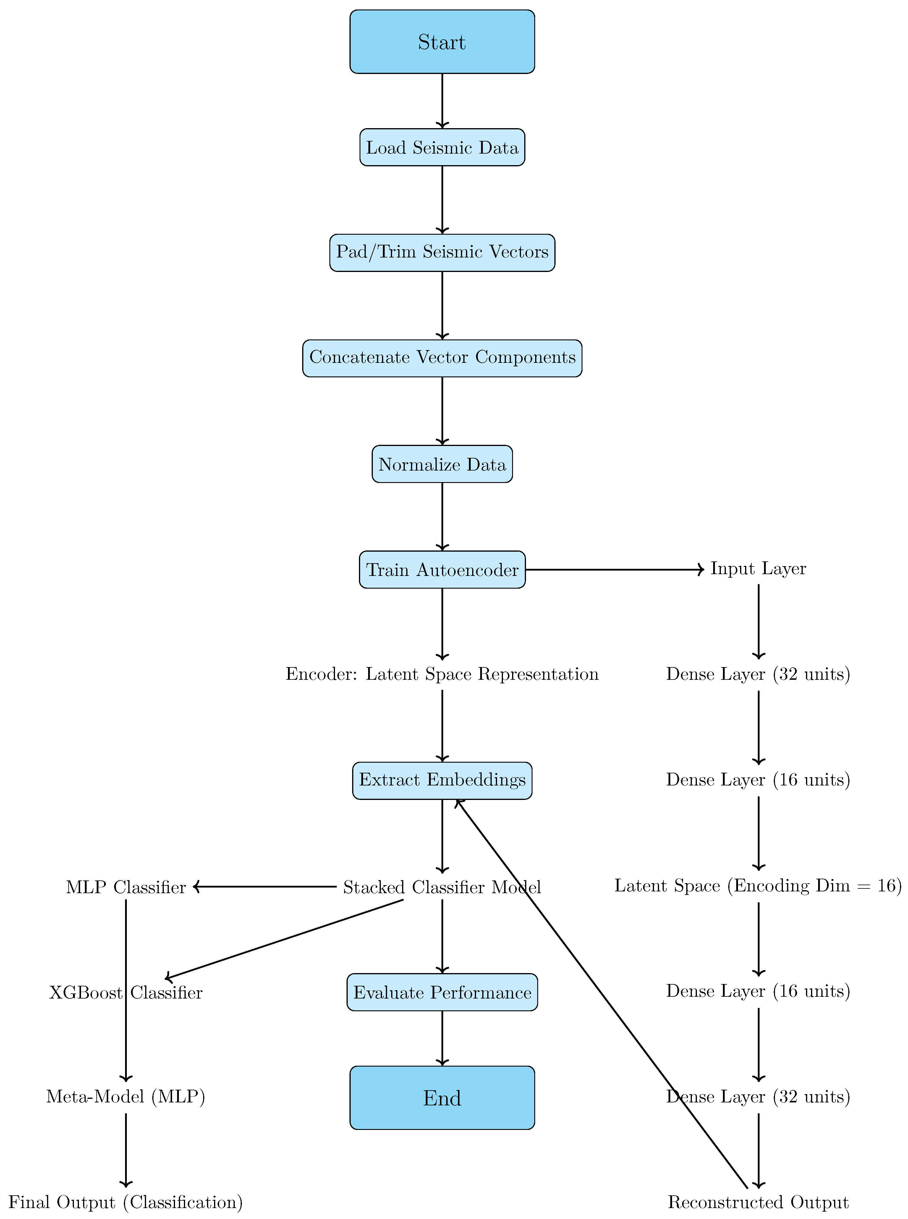
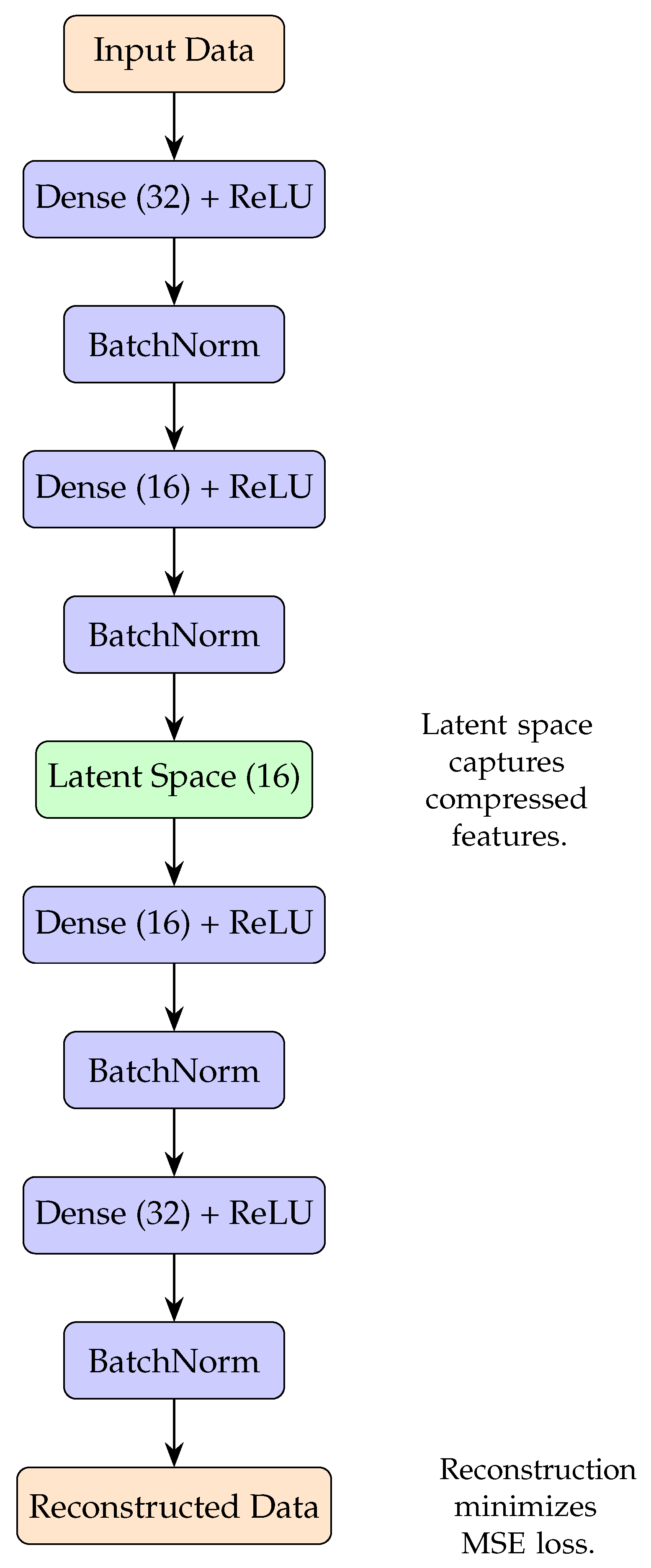
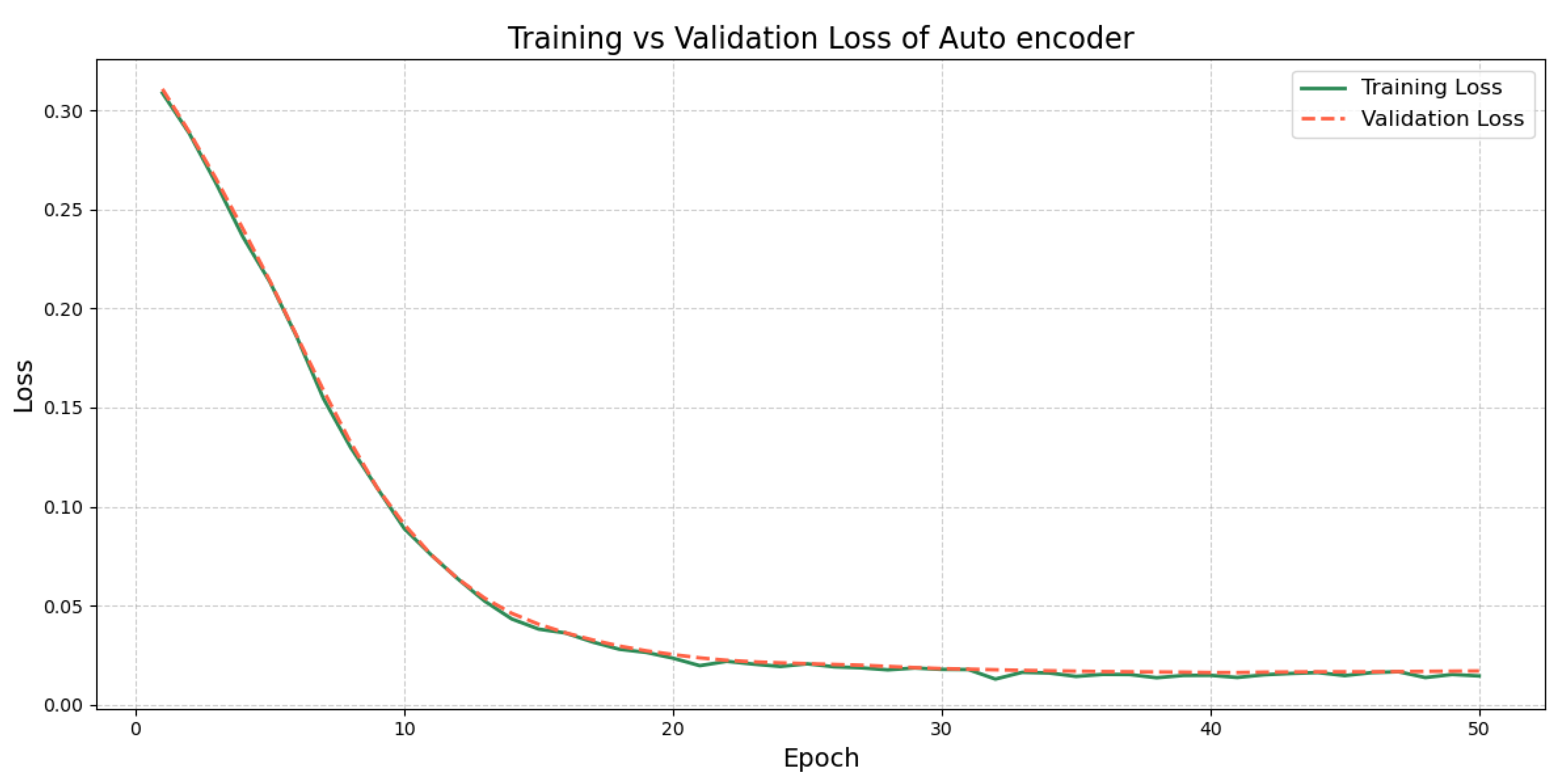
• Feature Extraction with an Autoencoder: An encoder has used ReLU activations to compress complex microtremor data and give more amplitude to the subtle pattern related to liquefaction.
• Robust Learning with Regularization: Batch normalization ascertains that the model will not overfit features, focusing only on the rare signal of liquefaction.
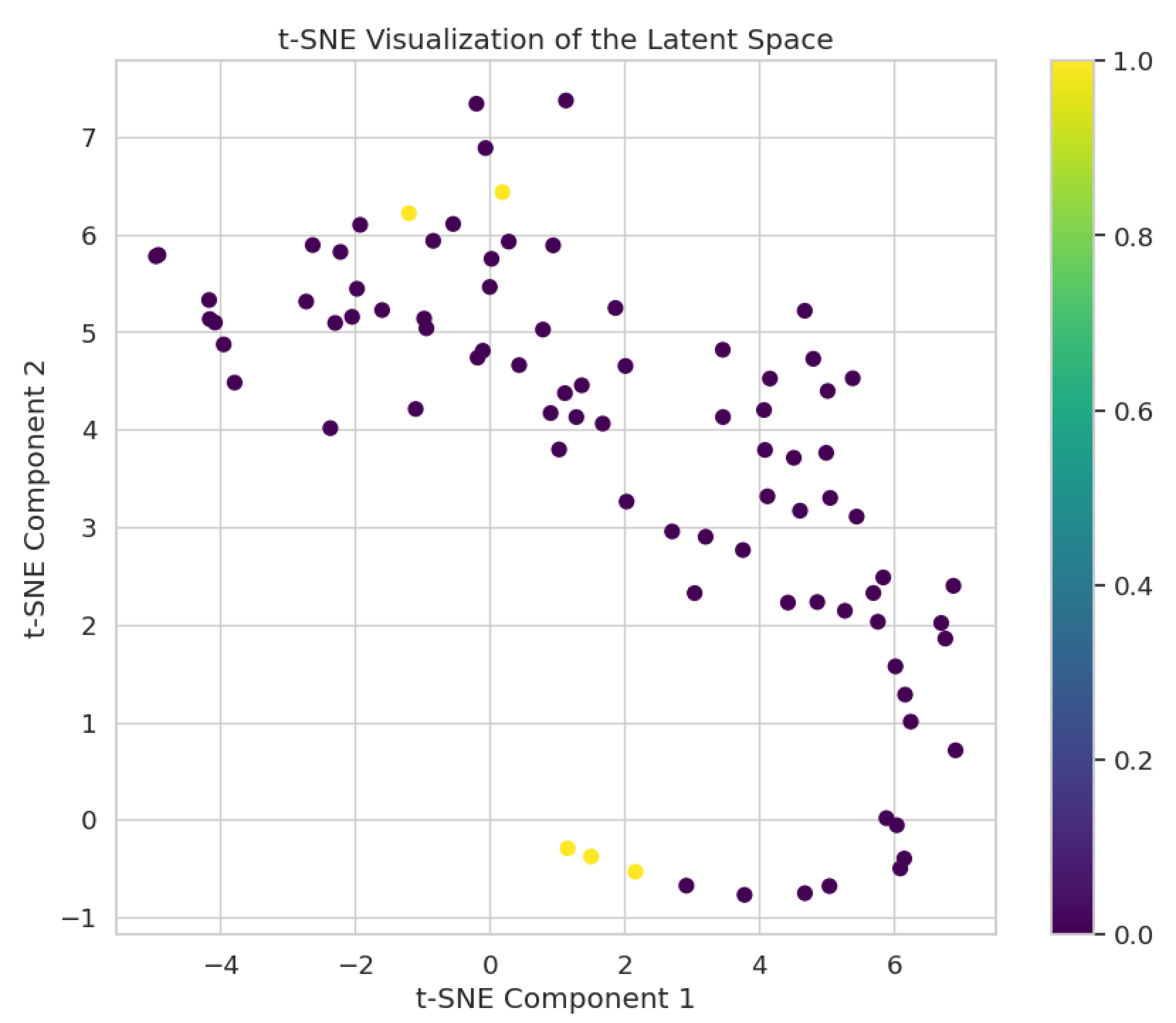
• Latent Space Embeddings: Critical indirect factors of liquefaction are caught by a latent 16-dimensional space, showing inner patterns of data.
• Stacked Classifier Ensemble: A stacked classified enseble combines the complex relationships identified by MLPwith the handling of class imbalance treated using XGBoost to make sure that the diversity within the data is reflected.
• Intelligent Meta-Model Aggregation: The final meta-model of MLP refines base model outputs, providing high priority to the rare events of liquefaction that may be missed in the individual models.
• Bias Mitigation by Representation Learning: The strengths of an autoencoder with embeddings and a stacked classifier are combined to avoid biases in concentrated datasets to represent liquefaction occurrence for rare data distributions.

This paper proposes a model that capitalizes on the advantages of autoencoders and stacked classifiers, boosting detection for such rare liquefaction events, even in the most hazardous seismic area of the Rif region of Morocco. Therefore, the proposed model is a potential tool for geophysical risk assessment and preparedness, offering an alternative to traditional approaches.

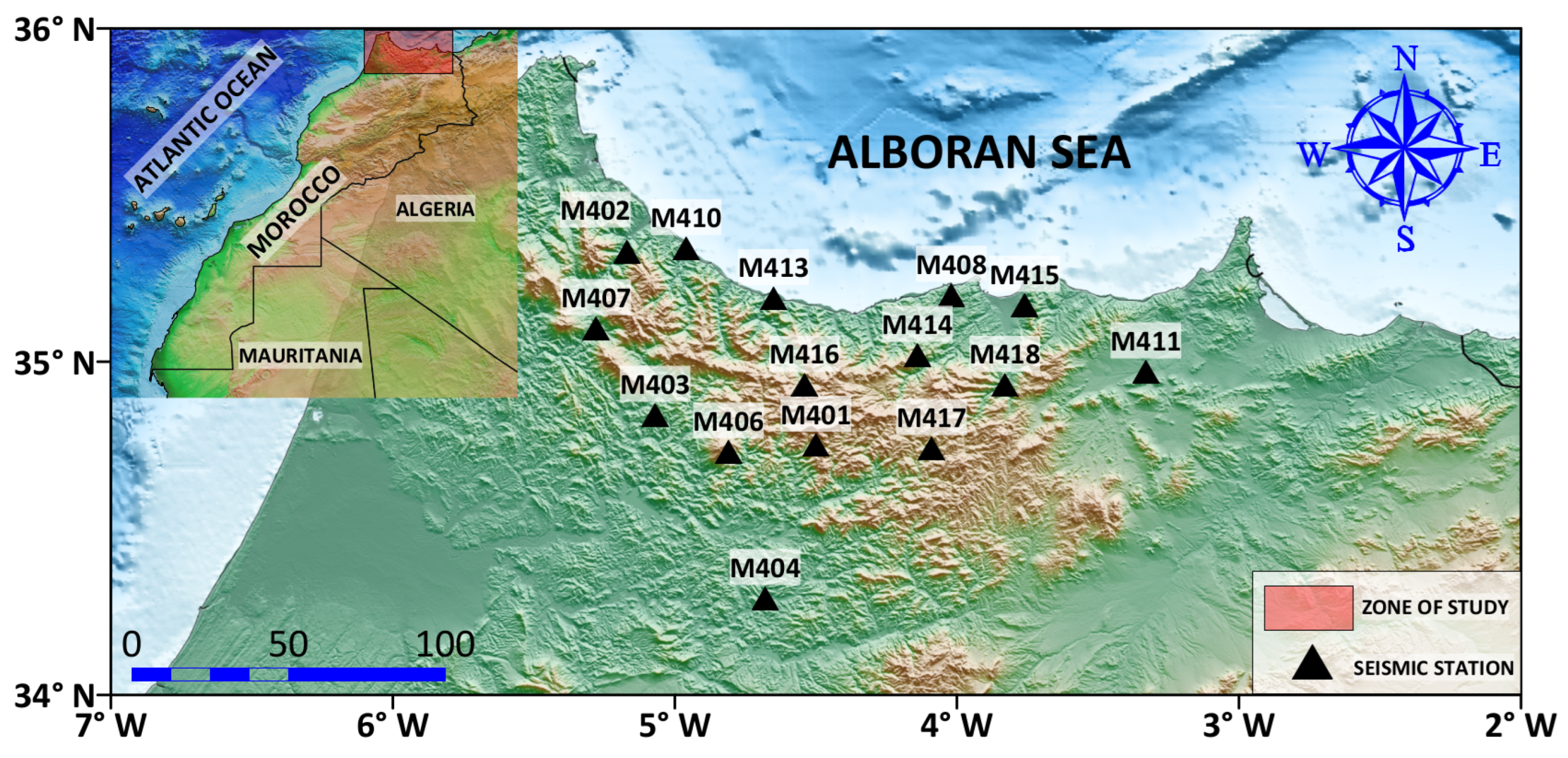
2. Geographical Setting

The region of the Rif sits in the northernmost part of Morocco and stretches along the Mediterranean coast—specifically, the Alboran Sea. It extends from Tangier in the west to the Moulouya River in the east. The Rif region is mountainous and known as a rugged geological zone caused by a destructive seismic history. It forms the southern part of the Gibraltar Arc, which is geologically related to the Betic Cordillera neighboring Spain. The Alboran Sea to the north, the Atlantic Ocean to the west, and the Sebou Basin to the south form the territory’s boundaries.

The topography of the Rif zone features prominent peaks, with the maximum elevation reaches approximately 2455 m in the Taza Al Hoceima region [31].

This region incorporates miscellaneous geological units such as the Internal Rif, which comprises metamorphic and igneous rocks geologically linked to the Alboran domain, Maghrebian Flyshchs, a sequence of sedimentary debris that operates as an intermediary bridge point between the Internal and External Rif, while the External Rif is essentially founded on sedimentary deposits from the Mesozoic and Cenozoic periods [32].

3. Methodology

The developed framework effectively incorporates current methods for geophysical data processing combined with machine learning to extract meaningful features from seismic microtremor data using the HVSR [33]. First, we handle the special analyses, especially for seismic data recorded by a plurality of stations, via steps needed to convert the data into raw form to gain further insights. Each step shifts the data closer to its ultimate purpose, providing critical features for predictive modeling, especially for site characterization in geophysical applications.

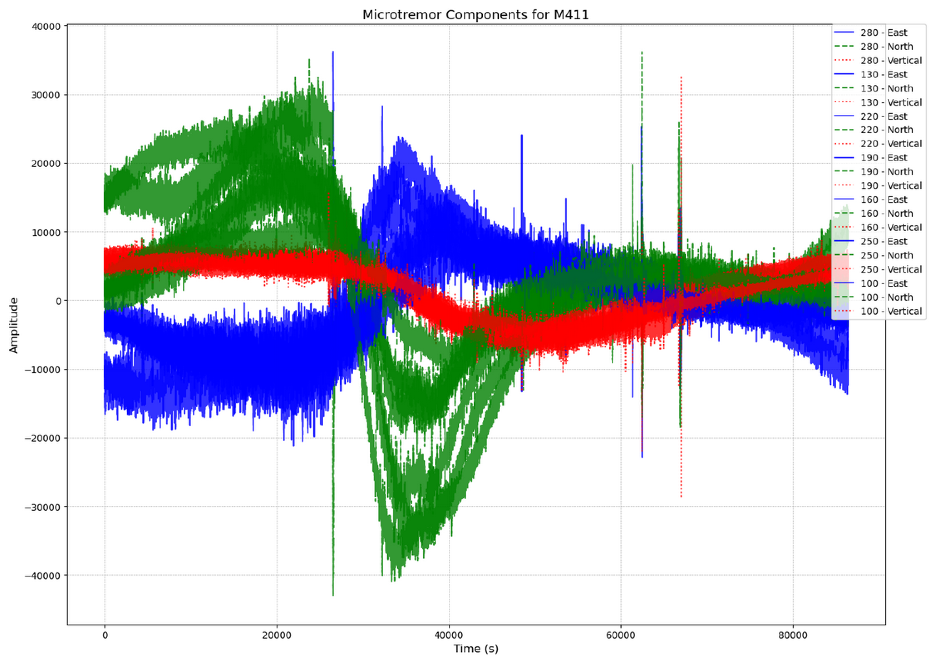
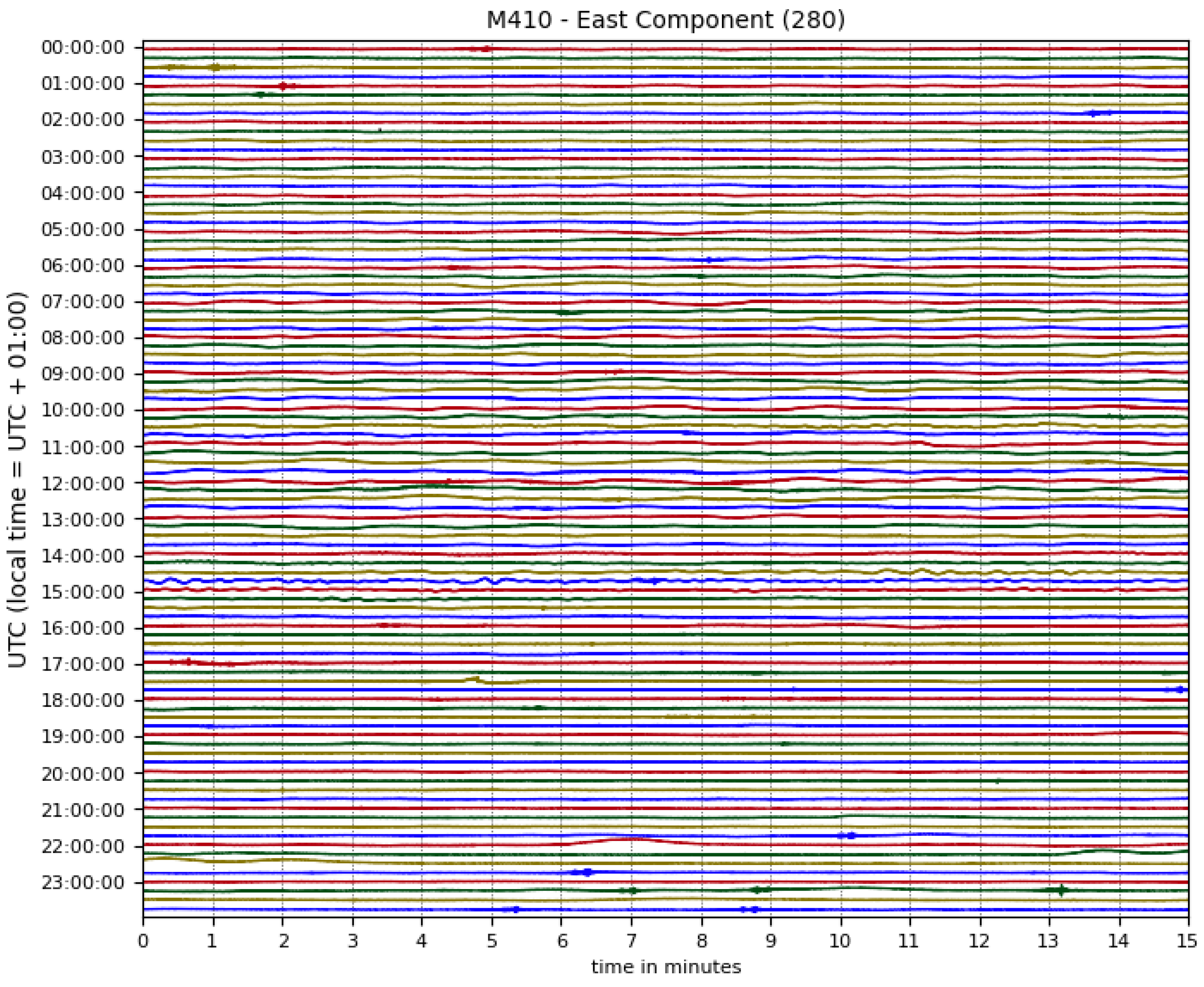
3.1. Data Acquisition and Preprocessing

The approach started with the loading of raw seismic data recorded from three orthogonal components, namely East (E), North (N), and Vertical (Z), for each station on a given day. Then, we read data using the obspy library, which is well known for its efficiency in handling seismic time-series data. Data were then arranged properly for each station in chronological order, supported by a strict naming convention, enabling us to find every seismic event and process them coherently.

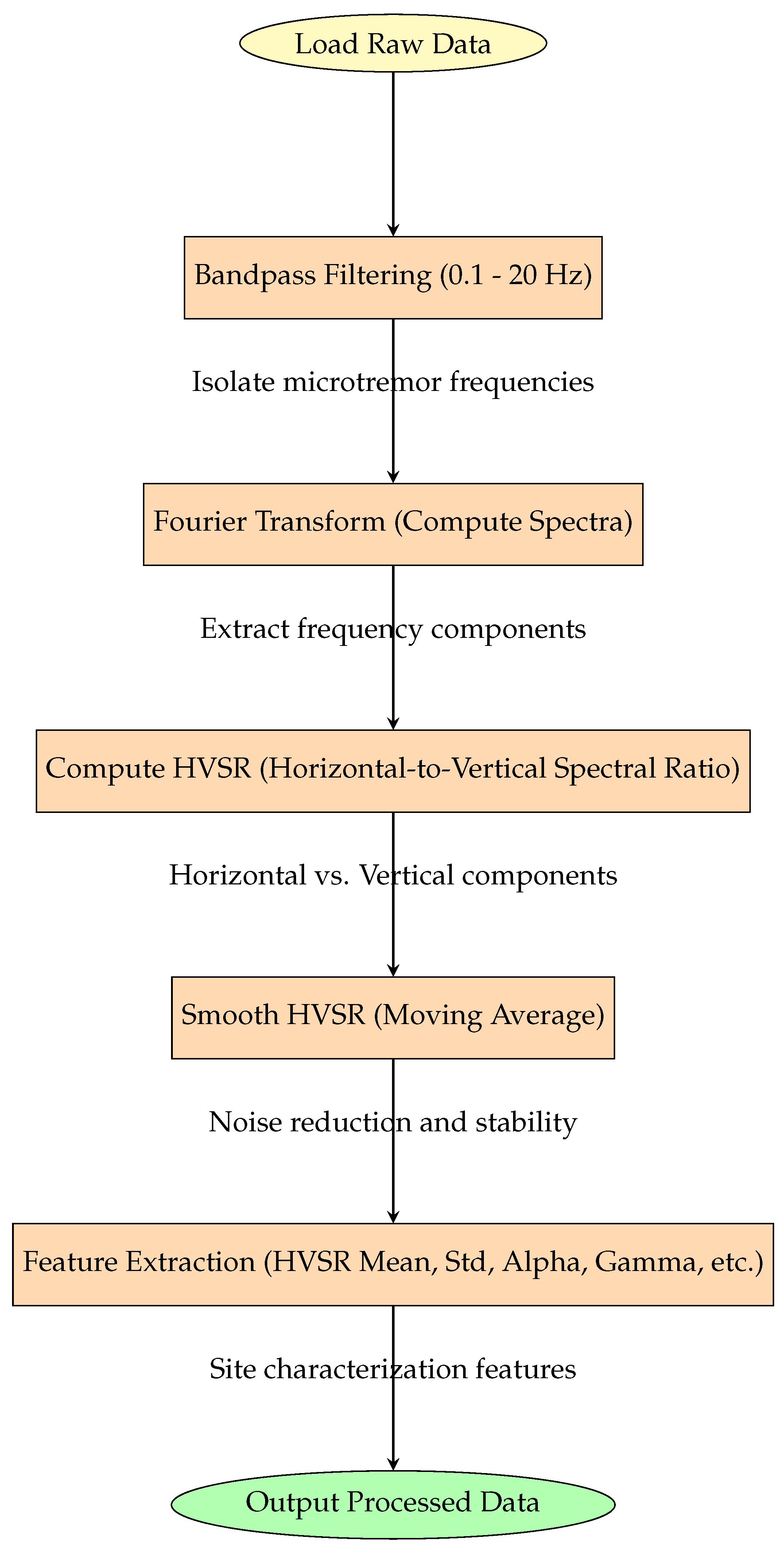
3.2. Bandpass Filtering

A critical filtering operation, namely bandpass filtering, was performed on the raw seismic data, to which we applied a Butterworth filter [34]. This filtering step is important because it enhances relevant low-frequency seismic noise to probe subsurface characteristics. Through its precise frequency attenuation, the filtering process allows the data to reflect subtle seismic oscillations, which are integral to the HVSR analysis, while filtering out the unwanted higher-frequency noise.

3.3. HVSR Computation

The analysis primarily focuses on the HVSR method for extracting subsurface features from seismic data. Site amplification and resonance effects are measured by the HVSR, comparing horizontal seismic motions along the East and North components to the vertical motions. We used Fourier transformation for its computation, which changes filtered components from time-domain to frequency-domain representations. We obtained the horizontal motion spectrum as the vector sum of the East and North components. Then, we obtained the HVSR from the ratio of the horizontal spectrum computation to the vertical spectrum. This ratio was then smoothed with a moving-average filter to reduce high-frequency noise and to stabilize the result [33,35].

The microtremor data comprised continuous daily recordings gathered throughout the year 2014. To ensure data quality, we performed an STA/LTA (Short-Term Average/Long-Term Average) method across each signal to analyze and validate signal stability and exclude noise-dominated segments. For windowing, we utilized a dynamic technique based on signal stability, choosing segments where the STA/LTA ratio showed persistent and dependable tremor activity. Additionally, each window needed to be longer than ${\displaystyle \frac{10}{f0}}$, guaranteeing that a minimum of 10 complete cycles were collected to facilitate robust frequency-domain analysis. We emphasize that both time-domain (e.g., peak amplitudes) and frequency-domain (e.g., HVSR peak and fundamental frequency ($f0$)) metrics were input for the machine learning models.

3.4. Feature Extraction

Accompanying this is a host of geophysical features extractable from the HVSR spectrum, with important insight each into the seismic behavior of the site [36]. In particular, these include the following:

• The amplitude spectra are obtained via Fast Fourier Transform (FFT):

  $$A_x\left(f\right)=\left|\mathrm{FFT}\left(x\right(t\left)\right)\right|\mathrm{for}x=e,n,z$$
• The HVSR (hvsr_ratio) is the ratio of the horizontal spectral components (East–West and North–South) to the vertical component.

  $$\mathrm{hvsr}\_\mathrm{ratio}\left(f\right)={\displaystyle \frac{\sqrt{{\left(A_n\left(f\right)\right)}^2+{\left(A_e\left(f\right)\right)}^2}}{A_z\left(f\right)}}$$

  where
  - $A_n\left(f\right)$ is the amplitude spectrum of the North–South component;
  - $A_e\left(f\right)$ is the amplitude spectrum of the East–West component;
  - $A_z\left(f\right)$ is the amplitude spectrum of the vertical component.
  Then, this ratio is smoothed using a moving average with a kernel of size 10:

  $$\mathrm{hvsr}\_\mathrm{smooth}\left(f\right)={\displaystyle \frac{1}{10}}\sum _{i=-5}^5\mathrm{hvsr}\_\mathrm{ratio}\left(f_i\right)$$
• Mean and Standard Deviation of HVSR: Shapes and variability in the overall HVSR curve provide critical information on resonance and amplification phenomena of the site.
  The mean of the smoothed HVSR ratio is expressed as follows:

  $$\mathrm{hvsr}\_\mathrm{mean}={\displaystyle \frac{1}{N}}\sum _{i=1}^N\mathrm{hvsr}\_\mathrm{smooth}\left(f_i\right)$$

  where N is the total number of frequency points.
  The standard deviation of the smoothed HVSR is expressed as follows:

  $$\mathrm{hvsr}\_\mathrm{std}=\sqrt{{\displaystyle \frac{1}{N}}\sum _{i=1}^N{\left(\mathrm{hvsr}\_\mathrm{smooth}\left(f_i\right)-\mathrm{hvsr}\_\mathrm{mean}\right)}^2}$$
• Alpha and gamma are parameters derived as the logarithmic and direct ratio, respectively, between the amplification factor and the fundamental frequency of the site; these are important in interpreting the dynamic resonance characteristics of the site.

  $$Alpha={\displaystyle \frac{{\log }_{10}\left(A_f\right)}{{\log }_{10}\left(f_0\right)}}\mathrm{if}{f}_0>0$$

  $$Gamma={\displaystyle \frac{A_f}{f_0}}\mathrm{if}{f}_0>0$$
• Z represents the energy distribution between horizontal and vertical components of microseismic waves to provide an integrated view of wave characteristics.

  $$Z={\displaystyle \frac{{\sum }_i{A}_h\left(f_i\right)}{{\sum }_i{A}_z\left(f_i\right)}}$$

  where

  $$A_h\left(f_i\right)=\sqrt{{\left(A_n\left(f_i\right)\right)}^2+{\left(A_e\left(f_i\right)\right)}^2}$$
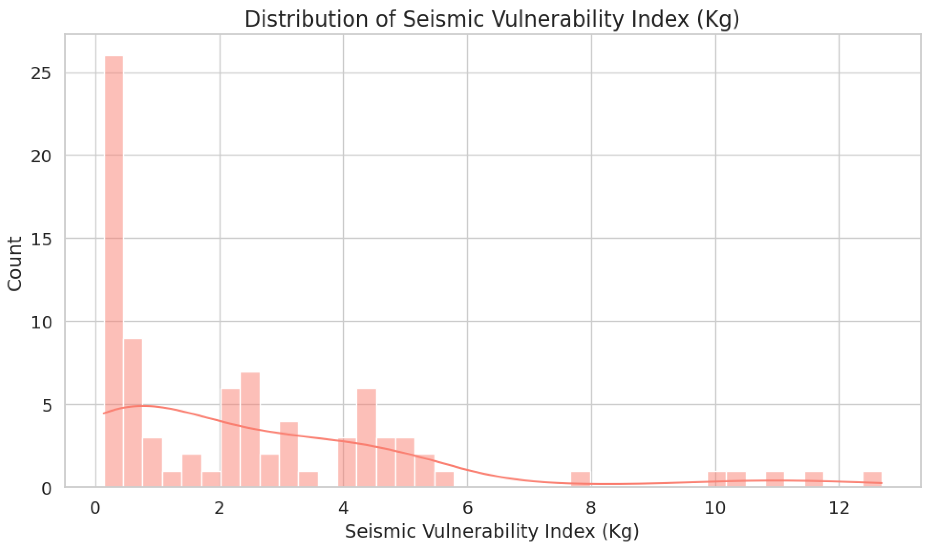
• The vulnerability index ($K_g$) is derived from the amplitude factor ($A_f$) and the resonant frequency ($f_0$), which provides more detail for the determination of spectral properties of the site.

  $$K_g={\displaystyle \frac{A_f^2}{f_0}}\mathrm{if}{f}_0>0$$

Features are extracted with the raw and filtered East, North, and Vertical components in the structured feature data. This process structures the features in a form that retains other critical information in a format known as a ‘rich feature’ set ready for deeper analysis, maintaining station identifiers, as well as the day of recording, fundamental frequency (f0), amplification factor (Af), and HVSR metrics.

Consequently, Figure 1 extracts key features from microtremor data. The essential core horizontal-to-vertical spectral ratio is calculated for six related processes, each contributing to the extraction and cleaning of seismic features.

First, the pipeline takes in raw seismic data from seismic stations, recording three basic components of motion, namely East, North, and Vertical, denoted as E, N, and Z, respectively. These are the minimum recorded measurements for data filtering. The raw data are filtered through a bandpass filter to isolate frequency ranges between 0.1 and 20 Hz where relevant seismic signals exist.

The successive steps involve Fourier transformation applied to the filtered data for all three components. It is a process in which a time-domain signal is decomposed into the frequency domain and presents the power of seismic data. The spectral representation then gives the variable frequency characteristics of the signal. Later, the HVSR juxtaposes horizontal motion, combining the East and North components with vertical motion. It also carries a significant amount of information about resonance and amplification at the site and reflects some subsurface properties of the seismic site.

Savitzky–Golay Smoothing [37,38]: Smoothing of the HVSR curve improves its interpretability by removing high-frequency noise using a moving-average filter; this stabilizes the HVSR and makes it more reliable. Features of different types are obtained from this smoothed HVSR, including statistical metrics of mean and standard deviation. Then, the derived parameters (alpha and gamma) describe the shape of the HVSR curve and its relation to the fundamental frequency and site amplification. These are crucial inputs in machine learning applications. The outcome after preprocessing is essential for further downstream analysis or integration into modeling workflows. The flowchart above represents a robust structured process, merging sophisticated signal processing with feature extraction in applications such as site characterization, seismic hazard analyses, and predictive modeling driven by machine learning.

3.5. Model Description

In this approach, we design jointly neural network-based feature extraction, ensemble learning, and sophisticated data preprocessing to construct a robust framework for microtremor event classification. The approach leverages unsupervised and supervised learning with imbalance dataset processing of relevant seismic features, enabling the classification of seismic events into their respective categories with high accuracy while preventing the model from overfitting to establish generalizability.

Figure 2 first takes raw seismic features in three filtered component vectors: East (E), North (N), and Vertical (Z). First, we unify vector sizes by padding or trimming them to some fixed length; in this approach, we choose 4. This ensures that the model treats every vector identically, regardless of whatever original length variability existed in the data. The pad_or_trim operationdoes this by adding zeros to the end of shorter vectors or truncating longer ones to make all inputs to the data identical in several dimensions before further processing. Finally, padded vectors for each seismic component are concatenated into one combined feature vector. This concatenation, itself, forms the basis of the neural network input, where each instance is represented as a flattened vector of the concatenated East, North, and Vertical components, enabling the model to learn complex relationships among them.

We use a standard scaler for feature data normalization by transforming the data to a standard normal distribution with zero mean and unit variance, making neural network training very stable.

We use an autoencoder, an unsupervised neural network usually trained for practical compression of an input, to extract a compressed representation of seismic data. At its core, are the autoencoder model comprises the following components: an encoder, a mapping that represents the input to a lower dimensionality latent space, and a decoder that reconstructs a compressed representation.

It captures structural features from the input and generates embeddings containing significant information about the input.

Figure 3 depicts the non-conventional approach to imbalanced data, with an encoder of a dense-layer rectified linear activation function (ReLU) that extracts features and compresses the input into a 16-dimensional latent representation; this models the complex and subtle relationships necessary for the identification of rare events of liquefaction. The use of a 16-dimensional latent space provides an acceptable compromise between compression and information preservation. Through exploratory trials, we discovered that fewer dimensions (e.g., <10) led to the loss of crucial information, whereas more dimensions showed modest performance benefits but increased complexity. Thus, 16 dimensions provide an adequate ability to capture crucial geophysical diversity without overfitting. BN helps prevent overfitting to more frequent features, allowing the model to learn how to detect less common patterns. The decoder rebuilds the input data from this compact embedding with a sigmoid output layer to ensure the reconstruction remains within the range of [0, 1]. However, the reconstruction loss is not directly related to liquefaction identification, leading the encoder to learn essential representations from the data. This is paramount in an imbalanced dataset, where the autoencoder pays more attention to the rare instances of liquefaction without bias towards the other classes, which occur more frequently. The increased ability to capture anomalies enhances the detection of liquefaction, thereby improving risk assessment and disaster preparedness in geophysical research.

The encoder part of the autoencoder consists of an array of dense layers, each followed by batch normalization for stabilization of learning and to prevent overfitting. Furthermore, it uses a latent space of 16 dimensions as a reflection of compressed representation in seismic data. Finally, we extract the embeddings from the encoder by using the trained model to predict the compressed features for each data point. These embeddings now represent the seismic data compactly, keeping only the most salient information and removing the noise. This stage is critical for reducing the size of the feature space and boosting computational efficiency and the capability of the model to learn robust patterns from the data.

We employed t-SNE visualization (Figure 4), which reveals unambiguous clustering of latent representations associated with label categories. This suggests that the compressed features represent significant, organized patterns connected to the underlying data. The t-SNE figure illustrates discrete clusters within the latent space, with the color denoting the value of the ‘Label’ column. The disparity between high and low label values from dark purple to yellow demonstrates that the model’s learned latent characteristics are meaningfully ordered and associated with the labels. Therefore, this gives weight to the hypothesis that the latent space includes essential, discriminative information.

The autoencoder-based model innovatively handles the challenge of traditional models that struggle with imbalanced datasets by learning a compact, 16-dimensional latent representation that captures key properties for liquefaction detection without being biased toward more prevalent soil conditions. Then, the generated embeddings from the autoencoder are fed as input for the next stacked classification model architecture, which includes an MLP classifier and an XGB classifier. The above base models capture intricate relations and patterns associated with liquefaction, even on imbalanced datasets. Consequently, the last meta-model also became another MLP classifier that combines the base model predictions in a wise balance between rare cases of liquefaction events. The goal of this stacking approach is to facilitate higher detection accuracy by combining several algorithms’ capabilities to improve effectiveness in finding odd events that might have been missed by individual models.

With the extracted embeddings, we start the classification stage with the aim of mitigating the class imbalance inherent in seismic datasets. In this direction, we employed a stacking ensemble that combines several base models for improved prediction. We combined Multi-Layer Perceptron (MLP) and XGBoost (XGB) classifiers. These base models make predictions used as inputs to feed into the final meta-model, which is an MLP, to yield the final prediction. The stacking approach allows a model to combine the strengths of an MLP for the modeling of complex nonlinear relationships with those of XGBoost for structured data with imbalances.

Another strategy is to assign class weights that penalize misclassifications of under-represented classes during training. The weight puts more importance on correctly predicting instances from the minority class, consequently turning out a model that is much fairer and more accurate.

Then, we evaluated different performance metrics of the proposed stacked ensemble model on imbalanced datasets. These metrics provide insight into a model’s ability to discriminate between classes.

We also trained a single, separate MLP model for benchmarking purposes. By taking its results and comparing them to the performance of the stacked ensemble model, we were able to measure the increase in performance.

Thus, the flowchart encapsulates a sophisticated, multi-step process of seismic data analysis, embedding, and deep learning with ensemble learning for microtremor classification. It involves some pre-processing of raw seismic data and padding or trimming to maintain a uniform vector length across the three components of East, North, and Vertical, followed by their concatenation into one feature vector; this vector then gets normalized and turned into a stable input for the succeeding autoencoder network. It acts as a nonlinear feature extractor that first compresses the data from the input in the encoder to a 16-dimensional latent space representation, then reconstructs it in the decoder phase. The decoder output provides embeddings that summarize the most striking features of the data for classification (Figure 3).

We used an autoencoder with the following properties: learning rate: 0.01; optimizer: Adam; batch size: 32; loss function: Mean Squared Error (MSE); and number of training epochs: 50. Figure 5 depicts the training and validation loss across 50 epochs. The training loss (shown in green) regularly stays somewhat lower than the validation loss (depicted as a red dashed line). The minimum difference between the two curves implies that the model learns successfully and generalizes well to unknown validation data.

These embeddings are input for the stacked ensemble model, an architecture that includes carefully chosen powerful base models: a multi-layer perceptron and an XGBoost classifier. This ensures that the model leverages complementary strengths from both algorithms. A meta-model combines these model outputs, and another MLP merges the base model predictions to provide an overall classification output. The resulting ensemble technique overcomes overfitting and, thus, adapts to complex, imbalanced datasets with robust performance. The model performance is evaluated using measures such as accuracy and the area under the receiver operating characteristic (ROC) curve (AUC), with applications in seismic hazard assessments, site characterization, and predictive geophysical modeling [39,40,41,42]. This work presents an innovative combination of deep learning and classical ensemble techniques, proposing a flexible and scalable model for different seismic applications. It describes a sophisticated mixture of signal processing, unsupervised feature extraction, and ensemble learning to conduct the difficult task of discriminating liquefaction potential classes in highly imbalanced datasets.

4. Experiments

We evaluate the model performance using several classification metrics:

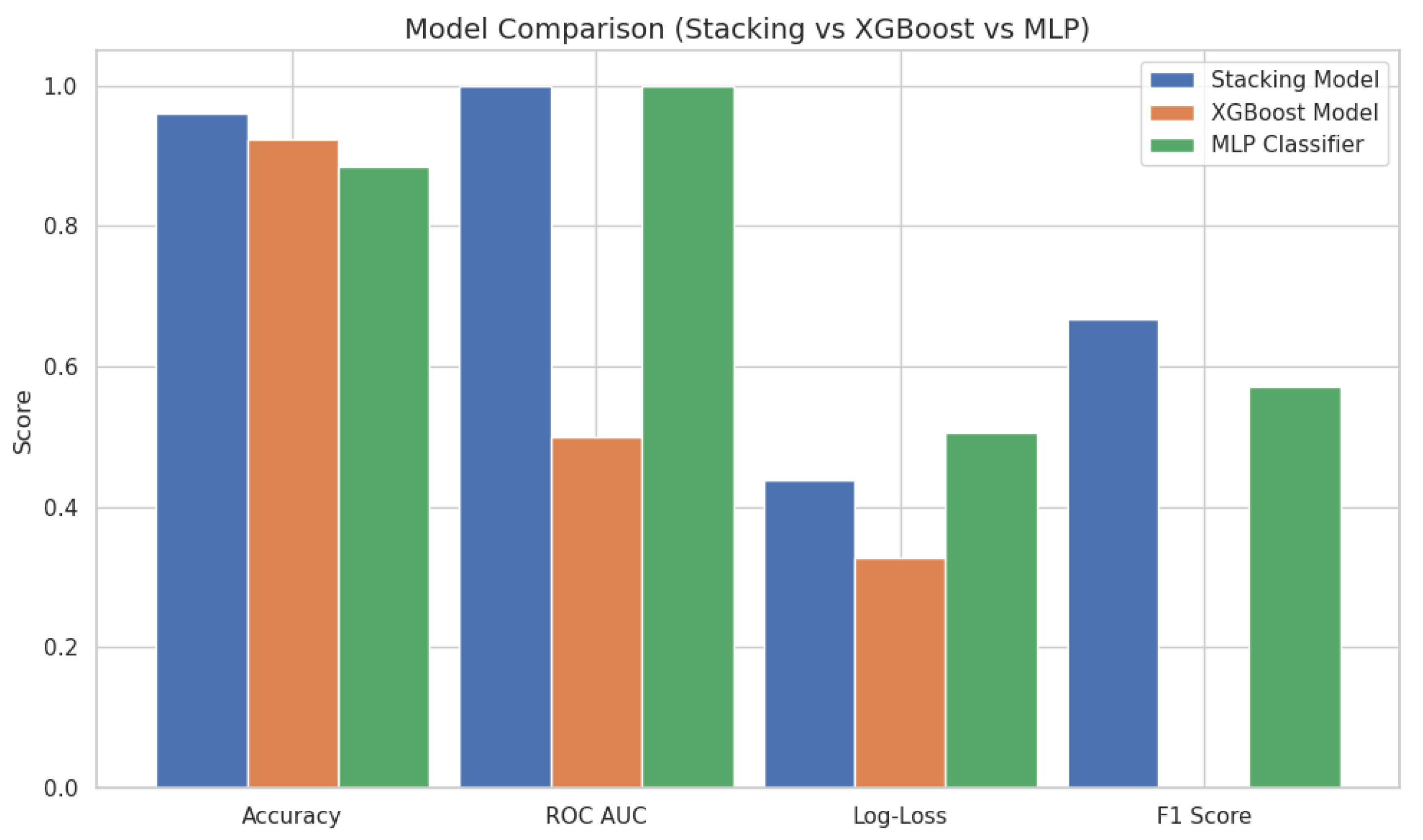
• Accuracy compares the total accuracy of the model as a ratio of true predictions to the total number of predictions.

  $$\mathrm{Accuracy}={\displaystyle \frac{\mathrm{True}\mathrm{Positives}+\mathrm{True}\mathrm{Negatives}}{\mathrm{Total}\mathrm{Samples}}}$$
• Precision estimates the number of predicted positives that are actually positive:

  $$\mathrm{Precision}={\displaystyle \frac{\mathrm{True}\mathrm{Positives}}{\mathrm{True}\mathrm{Positives}+\mathrm{False}\mathrm{Positives}}}$$
• Recall estimates how many actual positives were correctly identified by the model:

  $$\mathrm{Recall}={\displaystyle \frac{\mathrm{True}\mathrm{Positives}}{\mathrm{True}\mathrm{Positives}+\mathrm{False}\mathrm{Negatives}}}$$
• The F1 score is the mean of precision and recall, offering a balance between the two metrics:

  $$\mathrm{F}1\mathrm{Score}=2\times {\displaystyle \frac{\mathrm{Precision}\times \mathrm{Recall}}{\mathrm{Precision}+\mathrm{Recall}}}$$

4.1. Data Description

The data used in this research paper fits within the framework of the Topo Iberia Project [43], which was operated by the Scientific Institute of Rabat and the Jaume Almera Institute of Barcelona in 2007. The ubiquitous seismic network throughout the Rif territory (Figure 6) consists of 15 broadband stations implemented in 2014. In this study, we used microtremor measurement as an input to assess liquefaction using AI, as depicted in Figure 7 and Figure 8. The ground noise is modeled as a numeric microtremor signal registered by a Nanometrics Trillium 120P seismometer, which samples data at rate of 100 samples per second.

The dataset used for liquefaction identification comprised geophysical data obtained from the Rif region of Morocco, including various features—both qualitative and quantitative. Among the features, it is relevant to include meta-information about acquisition settings and filtering steps, namely Station, Days, e_filtered, n_filtered, and z_filtered.

The violin plot of amplitude ($Af$) versus liquefaction label compares two groups of data, non-liquefaction and liquefaction instances, with the distribution of amplitudes regarding liquefied and not-liquefied soil. As a result, non-liquefaction appears taller, with a broader mean, amplitudes that are more spread out, and a principal bulk ranging between 1.2 and 3.8. This indicates that the non-liquefied sites have a considerable amplitude range, and more of their data include points within this range. However, the liquefaction group is narrower and shorter because the distribution is more compact, lying between 2.5 and 2.9. this suggests that liquefaction-prone sites have a smaller, more consistent range of amplitudes, more closely clustered around the lower end of the scale. The plot showshow the amplitude behaves in sites that either liquefy or do not, providing information on possible seismic behaviors related to liquefaction risks (Figure 9).

The Seismic Vulnerability Index ($K_g$) is heavily concentrated at low values, indicating a dominance of stability and a landscape immune to seismic stress. But its long tail towards high values indicates sporadic anomalies, i.e., outliers that may represent fragile zones susceptible to collapse. The kernel density estimate subtly reflects the unpredictability of seismic behavior and shows fluctuations not evident with simple frequency counts. The spiky nature of the histogram bars at places shows localized instabilities, as if certain structural configurations make specific values of $K_g$ more likely to emerge. This suggests a hidden interplay of resilience, anomalies, and environmental stress distributions (Figure 10).

4.2. Results

The correlation matrix of features depicted in Figure 11 shows delicate relationships among the geophysical properties that control liquefaction risk. The hvsr_mean and hvsr_std are highly correlated, indicating that variability and the shape of resonance go together; sites with high resonance tend to show increased variability of seismic wave amplification, which may mean perilous vibration. The alpha parameter is less related to other parameters, providing information on harmonic behavior that does not directly relate to site density but is relevant to dynamic response estimation. The gamma parameter is highly correlated with $K_g$, indicating that sites with greater seismic amplification are more vulnerable to liquefaction. The negative correlation with $f0$ suggests that softer soils (lower fundamental frequency) tend to experience higher amplification, further increasing the liquefaction risk. The $K_g$ (vulnerability index) is strongly negatively correlated with f0, which means that lower fundamental frequency (softer, more liquefiable ground) is associated with a higher $K_g$. In other words, resonance increases dynamic response and increases liquefaction potential. The Z parameter is highly correlated with hvsr_mean and hvsr_std, which means liquefaction susceptibility is related to seismic energy amplification with both horizontal and vertical spectral components, so sites that have a more stable energy distribution or higher risk of amplification. Finally, the high correlation between Af and $K_g$ means high amplification factors, especially with lower f0 values, are at fault for liquefaction susceptibility. Finally, liquefaction susceptibility depends on the frequency, amplification, and energy distribution. The relationships among $K_g$, f0, Af, and Z necessitate a multi-dimensional methodology that accounts for the interplay of amplification and resonance with site dynamics to provide a comprehensive liquefaction hazard assessment.

We utilized 60 samples for training, with dimensions of (60, 24), where 24 denotes the number of features. The XGBoost model was configured with the following hyperparameters: n_estimators = 30, max_depth = 5, random_state = 42, use_label_encoder = False, and eval_metric = ‘logloss’. These parameters were set to balance model complexity and prevent overfitting, given the size of the dataset.

Figure 12 presents the confusion matrices of three classification models—MLP, XGBoost, and the proposed stacked model—for liquefaction and non-liquefaction event prediction. The confusion matrix provides an overview of the model’s accuracy.

The highest number of true positives and very few false negatives in the results of the best-performing stacked model showcase its ability to correctly identify and minimally misclassify events related to liquefaction. The true-negative and false-positive distributions are nearly balanced, indicating good results in non-liquefaction cases.

XGBoost, which ran second in performance, presents a slightly lower true-positive rate than the stacked model, implying more false negatives. Still, this model performed better than MLP, presenting fewer false positives and better handling of non-liquefaction events.

The worst was the MLP model, which had more false negatives and false positives. That is to say that the MLP model is not very efficient in detecting liquefaction events and misclassifies non-liquefaction events, showing its weakness in dealing with an imbalanced dataset.

Table 1. Model performance comparison. Support: number of samples in each class.

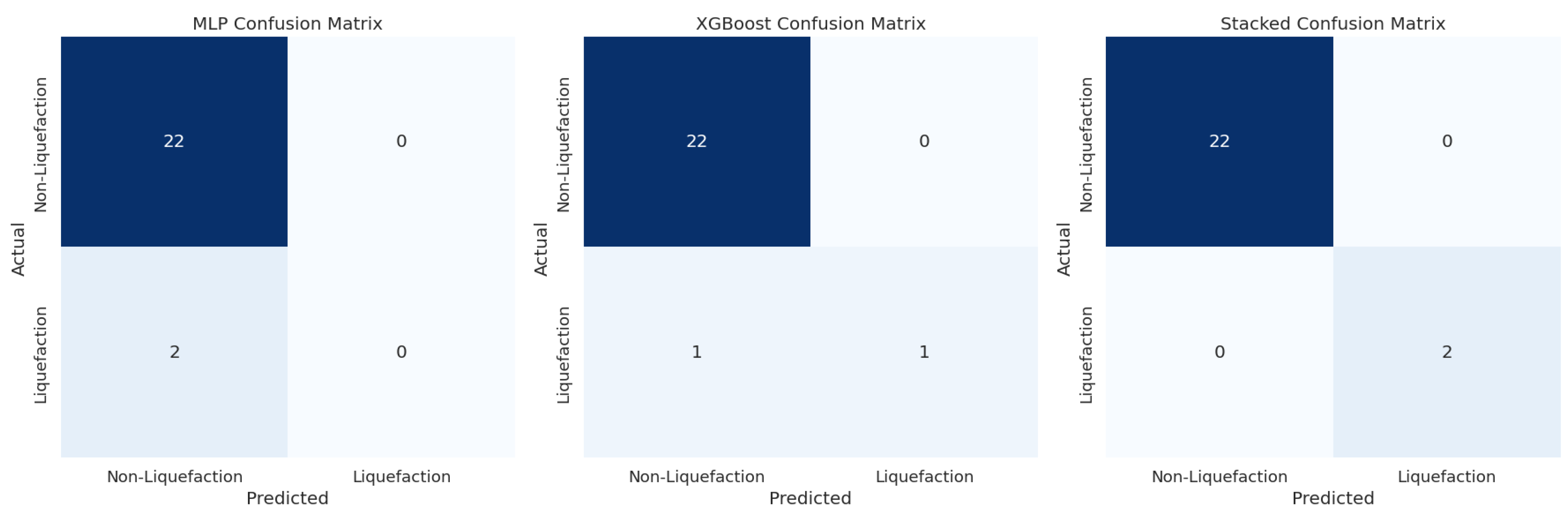
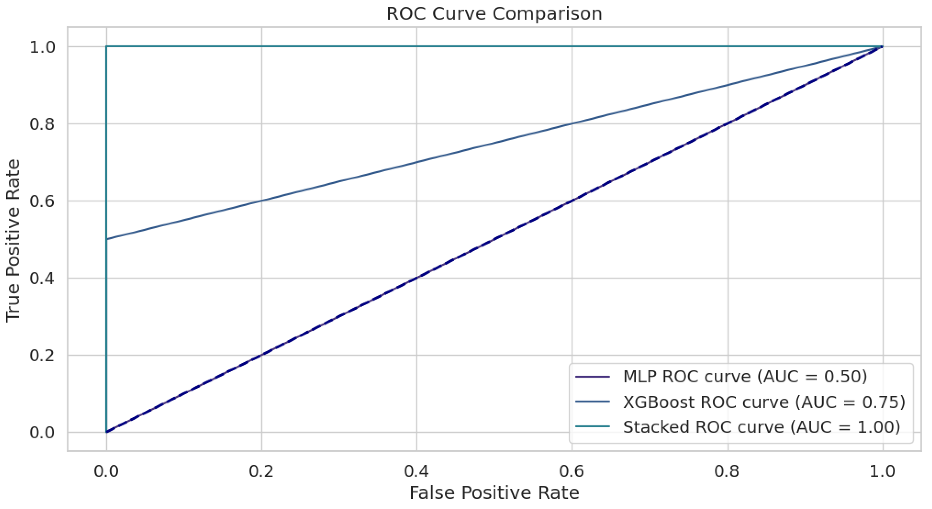
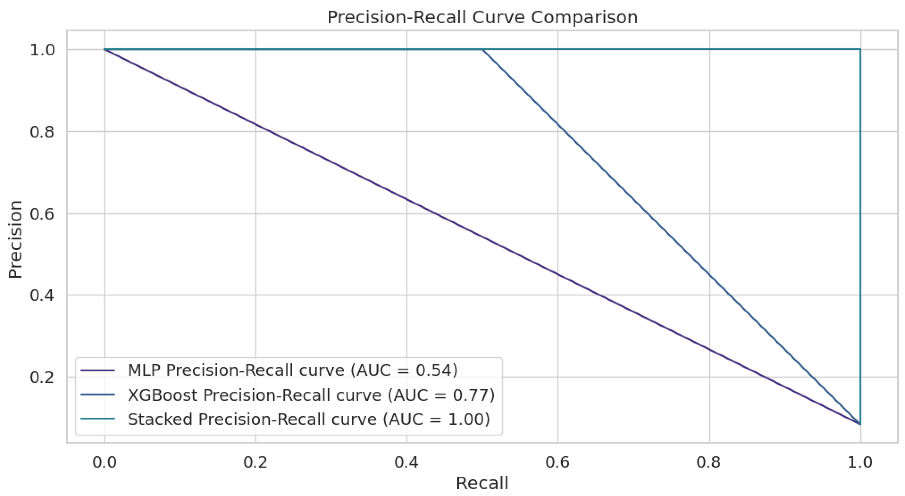
Model	Class	Precision	Recall	F1 Score	Support
MLP	0	0.92	1.00	0.96	22
	1	0.00	0.00	0.00	2
	Accuracy	0.92			24
	Macro Avg	0.46	0.50	0.48	24
	Weighted Avg	0.84	0.92	0.88	24
XGBoost	0	0.96	1.00	0.98	22
	1	1.00	0.50	0.67	2
	Accuracy	0.96			24
	Macro Avg	0.98	0.75	0.82	24
	Weighted Avg	0.96	0.96	0.95	24
Stacked Model	0	1.00	1.00	1.00	22
	1	1.00	1.00	1.00	2
	Accuracy	1.00			24
	Macro Avg	1.00	1.00	1.00	24
	Weighted Avg	1.00	1.00	1.00	24

highlights the classification accuracies of the MLP, XGBoost, and suggested stacking models. The stacking model demonstrates significant efficacy by integrating the attributes of several models, namely MLP and XGBoost, to overcome limitations that individual models cannot solve, especially in imbalanced categorization scenarios. Notwithstanding the deficiencies of the component models, including inadequate memory for the minority class and excessive focus on the majority class, the stacked model effectively capitalizes on the diverse predictions from both models to enhance overall performance. The stacking technique integrates various models, enhancing accuracy and recall by mitigating the biases and deficiencies of individual classifiers, yielding a balanced and robust output. This ultimately produces a model that surpasses other models on all metrics and demonstrates far more accuracy when integrated with a comprehensive solution than any individual model. This illustrates how the stacking method might enhance models’ generalization ability amid complex data distributions.

Figure 13 shows the MLP, XGBoost, and stacked models with their AUC values for performance evaluation. It is evident that the highest AUC is for the stacked model, proving that it achieves better classification performance by combining the powers of its base models effectively. The performance of XGBoost is not too bad but close enough, whereas MLP falls behind, which means there is still room for improvement. These results point toward the advantages of ensemble methods such as stacking in enhancing predictive power over individual models.

Figure 14 shows the PR curves of three models—MLP, XGBoost, and the stacked model—with AUC values to assess their performance on imbalanced data. The stacked model has the highest PR AUC, implying a better precision–recall trade-off, followed by XGBoost and MLP. Thus, the stacked model maintains high accuracy while maintaining high recall, making it the most effective for highly imbalanced data.

Figure 15 compares the results of the stacking model to MLP and XGBoost classifiers on four essential metrics: accuracy, ROC AUC, log loss, and F1 score. The stacked model outperformed the MLP and XGBoost predictors on most criteria, including accuracy, ROC AUC, and F1 score. However, it has a substantially smaller log loss than MLP but somewhat more than XGBoost. As a result, the stacked model performed better in general prediction and confidence, as it relied on its base models for higher accuracy and resilience when compared to class-balanced performance for the single MLP and XGBoost models.

Figure 16 shows the neuron counts vs. accuracy and loss of the stacked model over training epochs. The model with 64 neurons demonstrated the highest accuracy and least loss. This indicates that 64 neurons are at a better balancing point between the complexity and generalization of the model, such that the stacking model can catch underlying patterns more effectively while reducing overfitting. These results confirm the importance of choosing an appropriate number of neurons to ensure the best predictive performance for neural network architectures.

Figure 17 is a histogram comparing the distribution of the Stacking model’s probability against the predictions of the MLP classifier. The predicted probability values are more elevated at 0.4, with a higher peak density for predictions falling within this range, whereas in the MLP classifier’s distribution, the spread is more compact around a value of 0.5, with a lower peak density, and the prediction is scattered. From that, it follows that the tall and concentrated distribution of the stacking model represents a better ability to predict confidently and steadily. Thus, there is an improvement in predictive performance compared with the MLP classifier.

This distribution stands more elevated at 0.4 in the stacking model. It is within 0.18 to 0.6 range, signaling an assured and more focused behavior in prediction relative to the Kernel Density Estimation (KDE) depicted in Figure 18 for the predicted probability distributions of the stacking model and the MLP classifier. Contrasted with this is the distribution, peaking at around 0.5 in the same case, covered under a greater width for an instance of the MLP classifier, which says something about the confidence and variability of its prediction. The tall and focused distribution of the stacking model underlines, from another perspective, the superior capability of the stacking model to yield precise and reliable predictions compared to the MLP classifier.

To regularly test model performance across various conditions, a 1000-sample simulated dataset that mimics the Rif region containing equally distributed values within the observed minimum and maximum of each feature of the original dataset was established. This method preserves true geological and spectral behavior while maximizing unpredictability to more extensively explore the model’s response. Parameters such as the amplification factor (Af), fundamental frequency (f0), mean and standard deviation of the HVSR, seismic vulnerability index ($K_g$), alpha, gamma, and Z were considered in order to maintain site-specific parameters known to affect liquefaction. Filtered horizontal and vertical waveform components were also sampled to highlight waveform complexity. the constructed ‘depth’ variable enables the formulation of more physically consistent models of peak ground acceleration (PGA) and cyclic stress ratio (CSR). Liquefaction labels were assigned using an estimated CSR level of 0.15 according to prevailing technical standards. This methodology presents a realistic yet controlled test for model validation, and sensitivity analysis reduces risks of overfitting.

The confusion matrices for folds 1–5 show that the stacked model works well, making three to nine misclassifications per fold (Figure 19).

Stratified K-fold cross-validation maintained class balance, limiting bias and showing the model to be able to distinguish liquefaction from non-liquefaction events with high accuracy and recall.

A sensitivity analysis was implemented to validate stability. One-at-a-time (OAT) analysis (Figure 20) projected an amplification factor (Af) of $\tilde{0}$.059 and a seismic vulnerability index ($K_g$) of $\tilde{0}$.041 as the most sensitive parameters, both critical to CSR change.

Depth showed minimum sensitivity, with no significant contribution in the regional depth envelope. These findings were reinforced by the global Sobol sensitivity analysis, which indicates that Af and $K_g$ are significant factors, suggesting that model projections are influenced heavily by large physical inputs. Sobol first-order indices reveal that seismic vulnerability index components are of strong influence: $K_g$ (0.57), followed by Af (0.31), whereas depth has an extremely weak influence (0.01) (Figure 21).

The similarity of the two sensitivity methods enables reliance on rational model behavior and geographic transferability.

5. Discussion

The proposed hybrid model includes autoencoders and stacked classifiers in liquefaction identification with high perspective, imbalanced handling, and a geographical view of the geophysical data resulting from the Rif region. Indeed, most works on the issue of liquefaction detection adopt only basic approaches belonging either to a family of classification methods or to linear regression, whose shortcomings lie in handling an imbalances corresponding to minimal coverage of events such as liquefaction. While our model follows this route, it learns intricate relationships through feature extraction and uses ensemble methods to combine several learning algorithms’ points of view. The proposed model extends previous studies on autoencoders for unsupervised feature learning and also aligns with the work of Liu & Misra [44], who investigated how autoencoders capture nonlinear relationships in geophysical data while improving feature extraction in seismic studies. Based on the work of Ioffe & Szegedy [45], batch normalization plays a key role in our framework, stabilizing training and avoiding overfitting to dominant geological features so that rare liquefaction events are not ignored.

We integrated an ensemble classifier to enhance the predictive robustness of our approach. We combined nonlinear relationship modeling with MLP and handled class imbalance using XGBoost, following the work of Chen & Guestrin [46], who showed the efficiency of gradient boosting in classification tasks. However, most geophysical liquefaction models often suffer from missing environmental variables. Similarly, Vessia, Giovanna et al. [47] emphasized that local conditions, such as shear wave velocity and soil geometry, are critical in earthquake damage, even for sites very close to each other. Seismically induced soil deformations further influence damage outcomes. Therefore, it is useful to evaluate these factors in seismic risk mitigation, especially in cities, to enhance resilience in seismically active regions.

Class imbalance is still a barrier in liquefaction modeling, since rare liquefaction events cannot compete against more frequent geological occurrences. This fact, as pointed out by Sokolova et al. [48], leads to inflated overall accuracy at the expense of significantly worse performance regarding minority-class event detection. Our model, employing techniques such as batch normalization and an ensemble-based stacking classifier, overcomes this issue by being sensitive to these rare events of liquefaction.

Consequently, we can improve this model by including real-time seismic data or environmental inputs such as soil moisture changes caused by climate change. Although the autoencoder performs well in portraying raw data in compact form, much newer deep learning architectures like variation autoencoders and generative models might be considered in its place, apt for strengthening model learning of much subtler representations. This could extend the model further to include other seismically active regions where data and the distribution of influencing factors may vary, in addition to being helpful in bringing out its generalizability and robustness.

While the proposed model shows good performance, it suffers from some limitations. First, the real-world sample is small and highly unbalanced, with only two liquefaction cases, which reduces the statistical strength so that the model may not fully capture the range of field conditions. Although synthetic data were used to supplement training and measure generalizability, synthetic situations cannot perfectly mimic the complexity of real earthquake settings. Additionally, the model’s success may change when applied to different geographic regions or instrument setups. Future work should focus on increasing real-world data collection and proving the model across various regions and earthquake events.

Overcoming these limitations and further developing the current framework, our model could represent a more complete and scalable solution for liquefaction detection in the Rif region and other geophysical settings that may pose challenges.

6. Conclusions

This model is a powerful integration of state-of-the-art machine learning techniques for tackling challenges offered by imbalanced datasets, especially in the context of liquefaction identification in the Rif region’s geophysical landscape. An autoencoder distills complex geological patterns into a compact yet rich latent space, allowing for an emphasis on rare liquefaction events usually buried within the noise of more frequent, non-anomalous data. It capitalizes on the strength of an ensemble stacked classifier that merges the subtle capabilities of MLP and XGBoost, ensuring that subtle and rare liquefaction signals are recognized and prioritized.

In the case of the Rif region, where liquefaction occurrences are linked to peculiar tectonic and sedimentary conditions, this model performs better by learning nonlinear relationships and focusing attention on the interactions and complex interplay between features. Besides preventing overfitting, batch normalization and multi-model stacking decrease the bias toward the dominating classes, making the model more effective in discovering these rare geological catastrophes.

This approach could enhance the accuracy of liquefaction hazard assessment (hence, liquefaction hazard mapping) and could also optimize urban planning strategies. The results obtained by this approach can also assist decision-makers in selecting the types of interventions for this kind of hazard that could prevent life loss.

However, the model performs very well in identifying liquefaction from more general soil conditions based on existing geophysics features that might miss the state-of-the-art and less-used indicators of liquefaction risk. Furthermore, generalization from different geophysical environments is still an open issue, particularly outside the Rif region.

In the future, this model can incorporate other geophysical data, such as groundwater level, seismic velocity, and more detailed geological surveys. Furthermore, further research in advanced unsupervised learning techniques or real-time seismic monitoring data might result in an even better adaptive and accurate prediction. The study of the influence of the environment—for instance, climate-induced changes in soil—could also point in new directions with respect to the refinement of liquefaction risk assessments in dynamic, shifting areas like the Rif region.

References

- Marten Caceres, R.; Abrassart, T.; Boano, C. Urban Planning and Natural Hazard Governance; Oxford University Press: Oxford, UK, 2019. [Google Scholar]
- Bird, J.F.; Bommer, J.J. Earthquake losses due to ground failure. Eng. Geol. 2004, 75, 147–179. [Google Scholar] [CrossRef]
- Wani, K.M.N.S.; Mir, B.A.; Naik, T.H.; Farooq, M. Liquefaction mitigation by induced partial saturation: A comprehensive review. J. Struct. Integr. Maint. 2024, 9, 2429471. [Google Scholar] [CrossRef]
- Youd, T.L. Liquefaction-induced damage to bridges. Transp. Res. Rec. 1993, 1411, 35–41. [Google Scholar]
- Turner, B.; Brandenberg, S.J.; Stewart, J.P. Evaluation of collapse and non-collapse of parallel bridges affected by liquefaction and lateral spreading. In Proceedings of the 10th International Conference on Urban Earthquake Engineering, Tokyo, Japan, 1–2 March 2013; Tokyo Institute of Technology: Tokyo, Japan, 2013. [Google Scholar]
- Shafapourtehrany, M.; Batur, M.; Shabani, F.; Pradhan, B.; Kalantar, B.; Özener, H. A comprehensive review of geospatial technology applications in earthquake preparedness, emergency management, and damage assessment. Remote Sens. 2023, 15, 1939. [Google Scholar] [CrossRef]
- Pribadi, K.S.; Abduh, M.; Wirahadikusumah, R.D.; Hanifa, N.R.; Irsyam, M.; Kusumaningrum, P.; Puri, E. Learning from past earthquake disasters: The need for knowledge management system to enhance infrastructure resilience in indonesia. Int. J. Disaster Risk Reduct. 2021, 64, 102424. [Google Scholar] [CrossRef]
- He, X.; Chen, Z.; Yang, Q.; Xu, C. Advances in earthquake and cascading disasters. Nat. Hazards Res. 2025, 5, 421–431. [Google Scholar] [CrossRef]
- Poulos, S.J.; Castro, G.; France, J.W. Liquefaction evaluation procedure. J. Geotech. Eng. 1985, 111, 772–792. [Google Scholar] [CrossRef]
- Youd, T.L.; Perkins, D.M. Mapping liquefaction-induced ground failure potential. J. Geotech. Eng. Div. 1978, 104, 433–446. [Google Scholar] [CrossRef]
- Maurer, B.W.; Sanger, M.D. Why “AI” models for predicting soil liquefaction have been ignored, plus some that shouldn’t be. Earthq. Spectra 2023, 39, 1883–1910. [Google Scholar] [CrossRef]
- Yilmaz, C.; Silva, V.; Weatherill, G. Probabilistic framework for regional loss assessment due to earthquake-induced liquefaction including epistemic uncertainty. Soil Dyn. Earthq. Eng. 2021, 141, 106493. [Google Scholar] [CrossRef]
- Abbasimaedeh, P. Soil liquefaction in seismic events: Pioneering predictive models using machine learning and advanced regression techniques. Environ. Earth Sci. 2024, 83, 189. [Google Scholar] [CrossRef]
- Kim, H.-S. Geospatial data-driven assessment of earthquake-induced liquefaction impact mapping using classifier and cluster ensembles. Appl. Soft Comput. 2023, 140, 110266. [Google Scholar] [CrossRef]
- Phoon, K.-K.; Ching, J.; Shuku, T. Challenges in data-driven site characterization. Georisk Assess. Manag. Risk Eng. Syst. Geohazards 2022, 16, 114–126. [Google Scholar] [CrossRef]
- Wang, C.; Chen, Q.; Arduino, P. Data-centric seismic soil liquefaction assessment: Approaches, data, and tools. In Databases for Data-Centric Geotechnics; CRC Press: Boca Raton, FL, USA, 2024; pp. 427–451. [Google Scholar]
- Dieck, R.H. Measurement Uncertainty: Methods and Applications; ISA: Geneva, Switzerland, 2007. [Google Scholar]
- Kumar, D.R.; Samui, P.; Burman, A. Prediction of probability of liquefaction using hybrid ann with optimization techniques. Arab. J. Geosci. 2022, 15, 1587. [Google Scholar] [CrossRef]
- Ghani, S.; Thapa, I.; Kumari, S.; Correia, A.G.; Asteris, P.G. Revealing the nature of soil liquefaction using machine learning. Earth Sci. Inform. 2025, 18, 198. [Google Scholar] [CrossRef]
- Hu, J.; Wang, J.; Zhang, Z.; Liu, H. Continuous-discrete hybrid bayesian network models for predicting earthquake-induced liquefaction based on the vs database. Comput. Geosci. 2022, 169, 105231. [Google Scholar] [CrossRef]
- Jas, K.; Dodagoudar, G.R. Liquefaction potential assessment of soils using machine learning techniques: A state-of-the-art review from 1994–2021. Int. J. Geomech. 2023, 23, 03123002. [Google Scholar] [CrossRef]
- Kurnaz, T.F.; Erden, C.; Kökçam, A.H.; Dağdeviren, U.; Demir, A.S. A hyper parameterized artificial neural network approach for prediction of the factor of safety against liquefaction. Eng. Geol. 2023, 319, 107109. [Google Scholar] [CrossRef]
- Hameed, M.M.; Masood, A.; Srivastava, A.; Abd Rahman, N.; Razalid, S.F.M.; Salem, A.; Elbeltagi, A. Investigating a hybrid extreme learning machine coupled with dingo optimization algorithm for modeling liquefaction triggering in sand-silt mixtures. Sci. Rep. 2024, 14, 10799. [Google Scholar] [CrossRef]
- Alobaidi, M.H.; Meguid, M.A.; Chebana, F. Predicting seismic-induced liquefaction through ensemble learning frameworks. Sci. Rep. 2019, 9, 11786. [Google Scholar] [CrossRef]
- Khatti, J.; Fissha, Y.; Grover, K.S.; Ikeda, H.; Toriya, H.; Adachi, T.; Kawamura, Y. Cone penetration test-based assessment of liquefaction potential using machine and hybrid learning approaches. Multiscale Multidiscip. Model. Exp. Des. 2024, 7, 3841–3864. [Google Scholar] [CrossRef]
- Zhao, Z.; Duan, W.; Cai, G.; Wu, M.; Liu, S.; Puppala, A.J. Probabilistic capacity energy-based machine learning models for soil liquefaction reliability analysis. Eng. Geol. 2024, 338, 107613. [Google Scholar] [CrossRef]
- Ghani, S.; Kumari, S. Reliability analysis for liquefaction risk assessment for the city of patna, india using hybrid computational modeling. J. Geol. Soc. India 2022, 98, 1395–1406. [Google Scholar] [CrossRef]
- Li, P.; Pei, Y.; Li, J. A comprehensive survey on design and application of autoencoder in deep learning. Appl. Soft Comput. 2023, 138, 110176. [Google Scholar] [CrossRef]
- Riedmiller, M.; Lernen, A. Multi layer perceptron. In Machine Learning Lab Special Lecture; University of Freiburg: Freiburg, Germany, 2014; p. 24. [Google Scholar]
- Chen, T. Xgboost: Extreme Gradient Boosting. In R Package; Version 0.4-2; R Foundation for Statistical Computing: Vienna, Austria, 2015; Volume 1, pp. 1–4. [Google Scholar]
- Pateau, M. From hazard to natural risk: Tangier-tetouan region example (Rif, Morocco). Geo-Eco-Trop 2014, 38, 23–32. [Google Scholar]
- Arab, O.; Fellah, Y.E.; Harnafi, M.; Sebbani, J.; Abd el-aal, A.K. Estimation of the liquefaction potential in the region of Rif, Northern Morocco. Arab. J. Geosci. 2021, 14, 1–13. [Google Scholar] [CrossRef]
- Molnar, S.; Sirohey, A.; Assaf, J.; Bard, P.Y.; Castellaro, S.; Cornou, C.; Cox, B.; Guillier, B.; Hassani, B.; Kawase, H.; et al. A review of the microtremor horizontal-to-vertical spectral ratio (MHVSR) method. J. Seismol. 2022, 26, 653–685. [Google Scholar] [CrossRef]
- Oweiss, K.G. Statistical Signal Processing for Neuroscience and Neurotechnology; Academic Press: Cambridge, MA, USA, 2010. [Google Scholar]
- Xu, R.; Wang, L. The horizontal-to-vertical spectral ratio and its applications. EURASIP J. Adv. Signal Process. 2021, 2021, 1–10. [Google Scholar] [CrossRef]
- SESAME. Guidelines for the Implementation of the H/V Spectral Ratio Technique on Ambient Vibrations: Measurements, Processing and Interpretation; Technical Report, SESAME European Research Project WP12; Springer: Berlin/Heidelberg, Germany, 2004. [Google Scholar]
- Savitzky, A.; Golay, M.J.E. Smoothing and differentiation of data by simplified least squares procedures. Anal. Chem. 1964, 36, 1627–1639. [Google Scholar] [CrossRef]
- Vivó-Truyols, G.; Schoenmakers, P.J. Automatic selection of optimal savitzky- golay smoothing. Anal. Chem. 2006, 78, 4598–4608. [Google Scholar] [CrossRef] [PubMed]
- Gomez, B.; Kadri, U. Earthquake source characterization by machine learning algorithms applied to acoustic signals. Sci. Rep. 2021, 11, 23062. [Google Scholar] [CrossRef] [PubMed]
- Hasan, M.M.; Rahman, M.Z.; Fahim, A.K.F. Earthquake induced liquefaction hazard analysis for chittagong city using machine learning. Geomat. Nat. Hazards Risk 2025, 16, 2451126. [Google Scholar] [CrossRef]
- Ma, Z.; Mei, G. Deep learning for geological hazards analysis: Data, models, applications, and opportunities. Earth-Sci. Rev. 2021, 223, 103858. [Google Scholar] [CrossRef]
- Pilz, M.; Cotton, F.; Kotha, S.R. Data-driven and machine learning identification of seismic reference stations in europe. Geophys. J. Int. 2020, 222, 861–873. [Google Scholar] [CrossRef]
- Gárate, J.; Martin-Davila, J.; Khazaradze, G.; Echeverria, A.; Asensio, E.; Gil, A.J.; De Lacy, M.C.; Armenteros, J.A.; Ruiz, A.M.; Gallastegui, J.; et al. Topo-iberia project: Cgps crustal velocity field in the Iberian Peninsula and Morocco. GPS Solut. 2015, 19, 287–295. [Google Scholar] [CrossRef]
- Liu, R.; Misra, S. Machine learning assisted recovery of subsurface energy: A review. Authorea Prepr. 2022, 16, 6079. [Google Scholar] [CrossRef]
- Ioffe, S. Batch normalization: Accelerating deep network training by reducing internal covariate shift. arXiv 2015, arXiv:1502.03167. [Google Scholar]
- Chen, T.; Guestrin, C. Xgboost: A scalable tree boosting system. In Proceedings of the 22nd ACM SIGKDD International Conference on Knowledge Discovery and Data Mining, San Francisco, CA, USA, 13–17 August 2016; pp. 785–794. [Google Scholar]
- Vessia, G.; Laurenzano, G.; Pagliaroli, A.; Pilz, M. Seismic site response estimation for microzonation studies promoting the resilience of urban centers. Eng. Geol. 2021, 284, 106031. [Google Scholar] [CrossRef]
- Sokolova, M.; Japkowicz, N.; Szpakowicz, S. Beyond accuracy, f-score and roc: A family of discriminant measures for performance evaluation. In Australasian Joint Conference on Artificial Intelligence; Springer: Berlin/Heidelberg, Germany, 2006; pp. 1015–1021. [Google Scholar]