A Graph Isomorphic Network with Attention Mechanism for Intelligent Fault Diagnosis of Axial Piston Pump

Abstract

Axial piston pumps play a vital role in fluid power systems, which are widely employed in diverse fields such as aerospace, ocean engineering, and rail transit. It is essential to accurately diagnose faults in these pumps since their reliable operation hinges on it. A graph isomorphic network with a spatio-temporal attention mechanism (GIN-ST) is proposed in this paper for fault diagnosis of hydraulic axial piston pumps; GIN-AM addresses the problem of traditional intelligent fault diagnosis methods being limited to nonlinear mapping and transformation in Euclidean space. Initially, the weighted graphs are constructed from a univariate time series through K-nearest neighbor graph methods. Subsequently, a spatio-temporal attention-based module used to learn the graph representation of piston pump faults is presented, where a novel READOUT function and Transformer encoder provide spatial and temporal interpretability, respectively. Finally, the proposed (GIN-ST) model is compared against other intelligent fault diagnosis methods, and the superiority of the proposed method is proven.

1. Introduction

The axial piston pump is an essential component used to transmit power in hydraulic systems in various fields such as aerospace, rail transit, engineering machinery, and ship equipment. The failure of the axial piston pump can lead to severe safety hazards in equipment operation. The working conditions of axial piston pumps are typically harsh, with high levels of noise. Fault diagnosis in axial piston pumps can be challenging due to their concealed, coupled, random, and complex fault characteristics, making feature extraction and identification difficult. As a result, identifying an efficient and viable fault diagnosis method for axial piston pumps holds paramount importance in improving their performance.

Currently, fault diagnosis methods typically involve model-driven and data-driven approaches [1,2]. It is crucial to note that the model-driven methods establish a physical model, which reflects the device’s operational status based on its dynamic characteristics. However, this type of approach poses significant challenges due to its complex modeling process, which results in poor model universality. Conversely, data-driven methods do not require extensive knowledge of fault mechanisms [3,4]. With the growth of artificial intelligence, data-driven approaches rooted in deep learning made substantial progress in various domains, including, but not limited to, image processing, speech recognition, and fault diagnosis [5,6,7], and attracted widespread attention. Tang et al. [8] introduced a normalized convolutional neural network (NCNN) framework, leveraging batch normalization for both feature extraction and fault recognition in hydraulic pumps. These experiments revealed strong performance even in noisy environments. In recent times, the small sample ensemble intelligent fault diagnosis method was found to have remarkable applications in intelligent diagnosis in practical industrial scenarios, generating adversarial networks. The experimental results show that this method effectively improves the classification accuracy of bearing faults in situations where samples are limited [9]. However, axial piston pumps are complex electromechanical products with high integration, and ensuring their multisource information and generalized fault diagnosis remains a challenge [10]. As a result, data-driven approaches could fail to detect critical diagnostic information. DL only performs nonlinear mapping and transformation on Euclidean space, and it is therefore easy to overlook the interdependence between data [11].

Graph structure data contains a wealth of relational information that is distinct from image or voice signals and exists in non-Euclidean spaces. Currently, graph convolution neural networks (GNNs) focus more on data connectivity [12,13]. Traditional neural networks, such as CNNs, lack translation invariance within non-Euclidean structures (convolution kernels of the same size cannot be used for convolution) and can only analyze data in Euclidean space, disregarding the significant structural relationships of signals. This results in the loss of potential valuable information that can assist in distinguishing between failure modes [14]. Graph convolution networks (GCNs) revolutionized the processing of such data by enabling convolution operations on irregular graph structures. New solutions for the fault diagnosis of cross-coupled electromechanical products, such as that of axial piston pumps, are enabled by GCNs. Yu et al. [15] introduced a fast deep graph convolutional network (FDGCN) for diagnosing faults in wind turbine gearboxes, and their results demonstrate that the method achieves excellent fault classification ability and overcomes the noise problem of FDGCN by fusing traditional networks with graph convolution networks (GCNs). Good predictive performance was also achieved by deploying a deep graph convolutional network in the acoustic fault diagnosis of rolling bearings [16]. In response to the challenge posed by limited labeled data in industrial settings, a proposed intelligent fault diagnosis method for electromechanical systems introduces a semi-supervised graph convolutional deep belief network algorithm. The results depict high prediction accuracy with little labeled data [17]. The correlation of vibration signals at different time points is crucial in identifying and aggregating features to improve the prediction model’s robustness. Wei et al. [18] introduced an adaptive graph convolutional network (SAGCN) that utilizes a self-attention mechanism for feature correlation without a recursive function. The multi-scale deep graph convolutional network (MSDGCN) algorithm addresses the disordered fluctuations in the measured signal of the rotor-bearing system, demonstrating high accuracy and generalization [19]. The proposed graph isomorphic network (GIN) proves the graph structure’s representational capability while ensuring the integration of edge weights for different fault samples, resulting in an injective graph. The proposed model outperforms other machine learning models on all three real-world datasets [20].

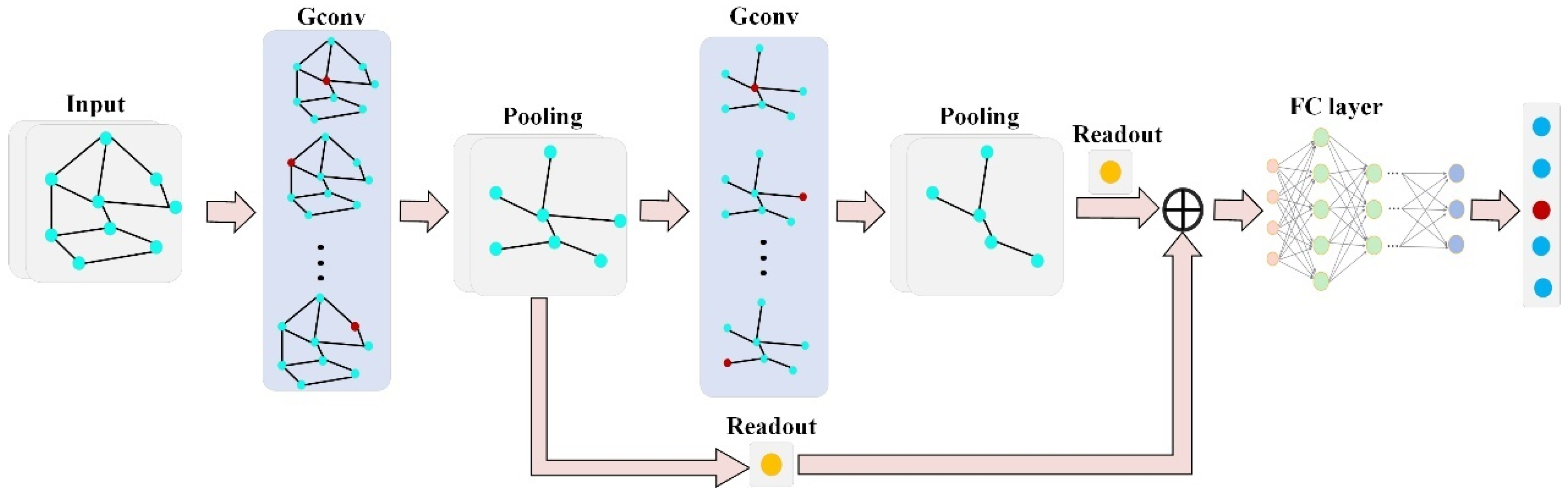
Current traditional GNN methods for fault diagnosis of complex electromechanical equipment, such as axial piston pumps, have poor classification accuracy, and lack temporal interpretability due to the dynamic characteristics of fault features in time series signals. GIN [21], is a variant of traditional GNN that was specifically designed for graph classification tasks. Inspired by the research work of previous scholars, a GIN with an attention mechanism is proposed in this article, in which a new attention-based READOUT module and Transformer encoder are designed to learn dynamic graph representations of different faults of axial piston pumps with spatio-temporal attention. The primary contributions of this paper include the following:

(1)

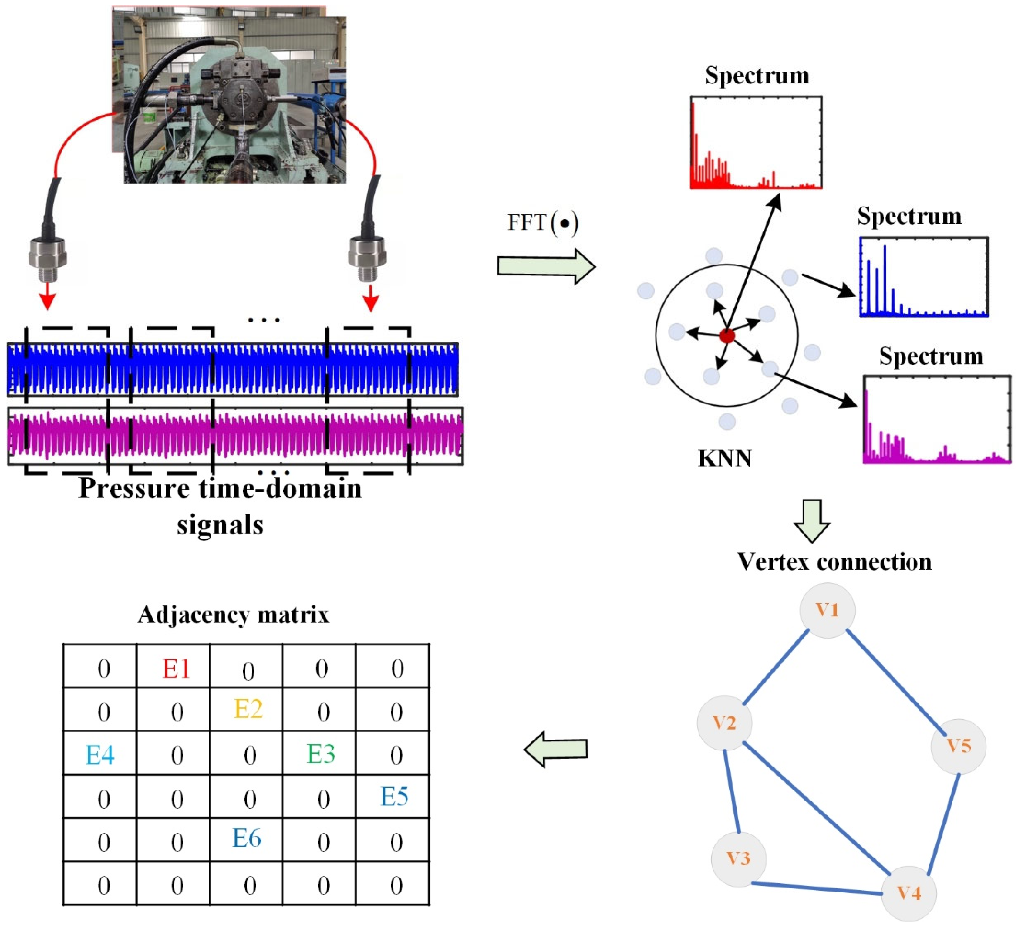
The relationship among input signals is gauged by transforming the raw signals into a weighted graph. Most current GCN implementations are built on unweighted graphs, despite the fact that, in reality, the importance of node neighbors often varies. By employing the weighted graph as the input, the proposed method (GIN-ST) exhibits a capacity to learn more comprehensive feature representations.

(2)

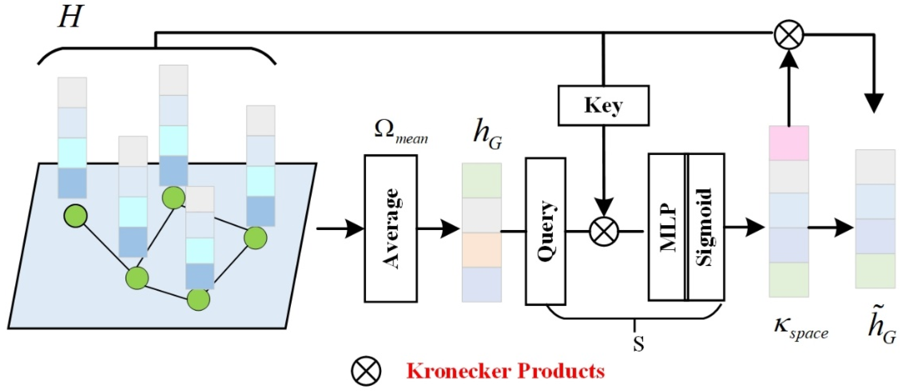
A novel attention-based READOUT module and Transformer encoder was devised in the present study. In contrast to conventional GIN networks, the designed READOUT module and Transformer encoder can decode deeper global features related to various faults in axial piston pumps. This enhancement markedly elevates the performance of the classification task, while concurrently affording spatiotemporal interpretability.

The paper’s organization follows a specific structure, beginning with the theoretical derivation of the graph convolutional networks (GCN) for diagnosing faults in axial piston pumps in Section 2. In Section 3, the proposed method is expounded upon, and Section 4 outlines the acquisition of experimental data for the axial piston pump. The subsequent Section 5 contains a discussion of the experimental results, and Section 6 provides a summary of the work in the concluding remarks. A brief flow of the proposed GIN-AM method for failure diagnosis of the axial piston pump is shown in Figure 1.

2. Graph Neural Networks

Graph neural networks (GNNs) integrate adjacency relationships and an extra dimension of information, often enhancing the model’s predictive performance. Figure 2 exhibits the architecture of the GNN for graph-level fault diagnosis, and the specific implementation procedure is described as follows:

2.1. Problem Definition

Let $G=(V,E)$ denote a graph with node feature vectors $X_v$ for $v\in V$, where $V$ is the set of vertices in the graph and $E$ is the set of edges connecting vertices in the graph. GNN utilizes graph structure and node feature $X_v$ to learn the representation vectors of node $h_v$ or the entire graph $h_G$. In GNNs, a neighborhood aggregation strategy is utilized, allowing the iterative update of representations for nodes via the aggregation of representations from neighboring nodes. The primary aim of this study is to conduct GNN training to optimize the representation of nodes.

$$f:G\to h_G$$

(1)

where $G=(G(1),\dots ,G(T))$ is a time signal sequence with T time points, and $h_G\in R^L$ is the vector representation of a graph. $f$ represents the linear mapping that needs to be learned.

2.2. Graph Isomorphic Network

GNN are typically composed of Aggregate and Combine functions [22], which determine the different variations in GNN.

$$a{a}_v^{(n)}=Aggregat{e}^{(n)}\left(\left\{h_u^{(n-1)}:u\in \mathcal{N}(v)\right\}\right)$$

(2)

$$h_v^{(n)}=Combin{e}^{(n)}\left(h_v^{(n-1)},a{a}_v^{(n)}\right)$$

(3)

where $h_v^{(n)}$ represents the feature vector of node $v$ at layer $n$ and $h_v^{(0)}:=x_v$.

The graph isomorphic network (GIN) is a significant variant of GNN. Traditional GNNs cannot efficiently discern features of two isomorphic graphs. The usage of sum aggregators instead of other functions enables GINs to learn more precise graph structure information. Thus, the sum aggregator serves as the AGGREGATE (•) function, followed by employing a multi-layer perceptron to model the COMBINE (•) function.

$$h_v^{(n)}=MLP\left(\left(1+{\Delta }^{(n)}\right)h_v^{(n-1)}+{\displaystyle \sum _{u\in N(v)}{h}_u^{(n-1)}}\right)$$

(4)

where $\mathrm{MLP}(\cdot )$ represents a multi-layer perceptron, where the learnable parameter, denoted by $\sigma$, is initialized to zero. To facilitate computations, Equation (4) can be expressed in a matrix format as follows:

$$H^{(n)}=\sigma \left(\left({\Delta }^{(n)}\cdot I+A\right)H^{(n-1)}{W}^{(n)}\right)$$

(5)

where the identity matrix is denoted as $I$, while $A$ refers to the adjacency matrix that captures the relationship between graph features, the MLP network weight is represented as $W$, and the variable $\sigma$ represents a nonlinear function.

The readout function in GIN uses updated node features $h_v^{(n)}$, and it can be written as follows:

$$h_G^{(n)}=Readout\left(\left\{h_v^{(n)}|v\in G\right\}\right).$$

(6)

The readout function here can be further represented in the following matrix form:

$$h_G^{(n)}=H^{(n)}{\Omega }_{\mathrm{mean}}$$

(7)

where ${\Omega }_{mean}^T=[1/N,\cdots ,1/N]$.

3. The Proposed Method

Section 2 of this paper highlights that the conventional READOUT function of GNN can be viewed as an unalterable decoder that deciphers the complete graph feature from the node features which are not adaptable. As a result, the issue at hand can be resolved by combining attention into the readout function, where attention denotes the scaling coefficient among nodes that are acquired through the model’s training process.

3.1. Graph-Attention READOUT

$H$ in Equation (8) can be used as a prior to calculate the spatial attention vector:

$${\kappa }_{space}=s(H)$$

(8)

$${\tilde{h}}_G={H\kappa }_{space}$$

(9)

where $\mathrm{s}(·)$ is attention function. ${\tilde{h}}_G$ is the spatial attention graph representation $h_G$.

Inspired by the attention mechanism, a novel attention-based readout function is designed. As presented in Figure 3, the attention-based readout module follows the Transformer’s attention based on key query embedding, with the key embedding calculated from the node feature matrix $H$, and the query embedding acquired from the unattended graph representation vector $H{\kappa }_{space}$.

$$\begin{array}{l}K=Q_{key}H\\ q=Q_{query}H{\Omega }_{mean}\\ {\kappa }_{space}=sigmoid\left({\displaystyle \frac{q^{T}K}{\sqrt{D}}}\right)\end{array}$$

(10)

where $Q_{key }\in R^{m\times m}$, $Q_{query }\in R^{m\times m}$ represents a key query parameter matrix that can be learned, and $K\in R^{m\times m}$ and $q\in R^m$ correspond to an embedded key matrix and an embedded query vector, respectively.

To enhance the classification accuracy and generalization capabilities of the GIN model, additional regularization techniques are applied to the adjacency matrix, including orthogonalization. In this regard, orthogonal regularization $L_{OR}$ is operationally defined as follows:

$$L_{OR }={‖1/n\cdot H^{T}H-I‖}_2$$

(11)

where $k=\max (H^{T}H)$. The scaling term $1/n$ preserves the orthogonality and equal length of the columns in the matrix H.

3.2. Transformer Encoder with Attention Mechanism

Due to the influence of a complex operating environment, the features of fault signals from axial piston pumps exhibit stochastic variations over time. To capture attention across time in the graph feature sequence (${\tilde{h}}_{G\left(1\right)},\cdots ,{\tilde{h}}_{G\left(T\right)}$), the final representation is generated by summing up these graph representations:

$$h_G=concatenate\left(\left\{h_G^{(n)}|n\in \{1,\dots ,N\}\right\}\right)$$

(12)

where $h_G$ is the concatenation of the graph representations of all $N$ layers.

3.3. Constructing Graphs from Time Series

The creation of weighted graphs is imperative for accurately representing the interactions between samples. Figure 4 demonstrates the step-by-step process for constructing weighted graphs, which involves data normalization of the original time series with a certain signal length. Subsequently, the time series data can be normalized as follows:

$$X^N=NOR(X)$$

(13)

where $X^N$ represents the normalized time series. NOR (·) refers to different normalization methods, and the maximum–minimum normalization method is employed [23].

Once data normalization is complete, the resulting values can be segmented into data samples of predetermined subsample lengths or dimensions $d$. This process yields a dataset that is ideal for further analysis and modeling:

$$\left\{\begin{array}{l}M=\left(x_1^{Nol},x_2^{Nol},\dots ,x_n^{Nol}\right),x_n^{Nol}\in X^{Nol}\hfill \\ n=floor \left({\displaystyle \frac{L}{d}}\right)\hfill \end{array}\right.$$

(14)

where $M$ is the constructed subsample set, $x_n^{Nol}$ denotes subsamples, $n$ is the total number of subsamples, $floor$ represents rounding to negative infinity, and $d$ is the size of the subsamples.

To mitigate the effects of environmental noise generated by axial piston pumps on graph features, we conducted fast Fourier transform (FFT) on each subsample, and viewed the resulting spectrum as a distinct sample. This process can be illustrated as follows:

$${\tilde{x}}_i=FFT\left(x_i^{Nol}\right),i=\mathrm{1,2}\cdots n.$$

(15)

The FFT refers to the process of converting subsamples to the frequency domain and then extracting the resultant frequencies. By assigning identical labels to each sample, a labeled dataset can be obtained:

$$D=\left[\left({\tilde{x}}_{1,}{y}_1\right),\left({\tilde{x}}_{2,}{y}_1\right),\cdots \left({\tilde{x}}_{n,}{y}_n\right)\right]$$

(16)

where $D$ is the labeled dataset.

To determine the top-k nearest neighbor for every node, a weighted graph can be generated using the aforementioned dataset. The resulting neighbors of node $x_i$ can then be written as follows:

$$Ne\left(x_i\right)=KNN\left(k^{\prime },x_i,\zeta \right)$$

(17)

where $k^{\prime }$ is taken as 5 in this paper. $\zeta =\left[x_{i+1},x_{i+2},\dots ,x_{i+m}\right]$ is a subset with $m$ samples, and $Ne\left(x_i\right)$ represents the nearest neighbor of node $i$. The edge weights between nodes in a weighted graph can be estimated using the Gaussian kernel weight function. This function is defined as follows:

$$e_{ij}=\exp \left(-{\displaystyle \frac{{‖\left(x_i,x_j\right)‖}^2}{2{\delta }^2}}\right),\hspace{1em}{x}_j\in Ne\left(x_i\right)$$

(18)

where $e_{ij}$ represents the edge weight between node $x_i$ and node $x_j$, while $\delta$ denotes the bandwidth of the Gaussian kernel.

4. Experimental Data Acquisition

4.1. Experimental Testing Platform for Axial Piston Pumps

This paper presents experimental investigations of a swash plate axial piston pump, as depicted in Figure 5a. The drive shaft is supported by front-end and rear-end bearings installed in the cover and shell, respectively. The rotor assembly comprises the cylinder block, pistons, and slippers, with the latter connected to their corresponding pistons via ball joints. The pistons, uniformly distributed around the center of the cylinder block, are essential components of the pump. The slipper pair, piston pair, and valve plate pair are three key interfaces in axial piston pumps, serving as a critical seal and support. These interfaces are crucial to the pump’s lifetime and reliability.

Figure 5b illustrates the test platform with three oil lines for the axial piston pumps: the input, leakage, and output lines. The pressure in the output line is regulated by a relief valve, and it significantly influences the pumps’ efficiency and performance. Therefore, the output pressure signals of the axial piston pumps are utilized as model inputs for failure diagnosis. A pressure transducer is used to measure the output pressure, and the data acquisition module collects the pressure signals with a sampling rate set at 65,536 Hz, while the data duration is 5 s. A detailed description of the test device is presented in

Table 1. Detailed descriptions of the test platform.

No.	Names	Descriptions
1	Electric motor	ABB-IEL-280M75
2	Axial piston pump	A4VSO40
3	Output pressure transducer	HM90-0~35MPa-H3V2F1
4	Relieve valve	DBW30B-1-50B/350bar
5	Data acquisition module	Type LAN-XI 3050, Brüel and Kjær,
6	Laptop	ASUS K450V with PULSE

.

Table 2. Technical specifications of the pressure transducer.

No.	Names	Descriptions
1	Transducer model	WIKA A-10 pressure transmitter
2	Pressure range	0–10 MPa
3	Accuracy	±0.25% full scale (FS)
4	Sampling frequency	10 kHz
5	Output signal	4–20 mA (converted via 16-bit ADC)
6	Impulse tube length	<200 mm

shows the specific models and parameters of the pressure sensors, which are mainly used to measure the flow pressure at the pump outlet.

Table 3. Detailed parameters of the axial piston pump.

No.	Names	Value
1	Rotating speed	1500 r/min
2	Maximum displacement	40 mL/r
3	Output pressure	21 MPa

displays the operating conditions of the test rig, which includes an electric motor rotating at 1500 r/min, axial piston pumps with a maximum displacement of 40 mL/r, and a pump output pressure of 21 MPa.

4.2. Health State Settings of Axial Piston Pumps

Figure 6 illustrates the six distinct health states of the axial piston pump: the normal piston pump (NOR), cavitation damage of the valve plate pair (CDV), slipper wear fault (SWF), piston wear fault (PWF), rolling element damage of the front-end bearing (RDFB), and rolling element damage of the rear-end bearing (RDRB).

In Figure 7, the corresponding time domain signals for each of these fault types are presented. The normal state, NOR, is characterized by a lack of any fault. Conversely, the CDV, SWF, and PWF represent fault states pertaining to the valve plate pair, slipper pair, and piston pair, respectively. Specifically, CDV is indicative of cavitation damage faults (1 mm in width) between adjacent piston holes on the cylinder block. SWF points to slipper wear faults (0.02 mm in wear along the thickness). PWF signifies piston wear faults (0.009 mm in wear along the diameter). Lastly, RDFB and RDRB denote rolling element damage affecting the front-end and rear-end bearings. In both cases, rolling element damage manifests as grooves 0.5 mm in width. A detailed overview of these states can be found in

Table 4. Detailed descriptions of different health states.

No.	Names	Descriptions
1	NOR	Normal
2	CDV	Cavitation damage of the valve plate pair
3	SWF	Slipper wear fault
4	PWF	Piston wear fault
5	RDFB	Rolling element damage of the front-end bearing
6	RDRB	Rolling element damage of the rear-end bearing

.

As illustrated in Figure 8, FFT analysis was carried out on a range of time domain pressure signals for various fault types associated with axial piston pumps, and the results show minimal differences in the spectral output between different fault types. These findings clearly suggest that when subject to significant background noise, a lack of significant variance in spectral features underscores the point that shallow spectral analysis of system data should not be solely relied upon as an accurate method of diagnosing potential faults.

To investigate the time–frequency spectrum of the output pressure signal, continuous wavelet transforms (CWT) were employed to convert six distinct health conditions into 2D time–frequency representations. In the signal pre-processing phase, the complex Morlet wavelet was selected as the basis function. This choice was made because of its ability to capture the signal’s characteristics through the amplitude and phase of the wavelet coefficients and its excellent interpretability.

The time–frequency spectrum of the six pump pressure signals is shown in Figure 9. There are strong similarities between the time–frequency representations for different fault types, with the frequency range and amplitude of different health states fluctuating within a narrow range. Therefore, it is difficult to accurately diagnose faults using the CNN method based on these images. As a result, it is necessary to employ a novel deep neural network to extract useful features and achieve reliable fault diagnosis.

5. Results and Discussion

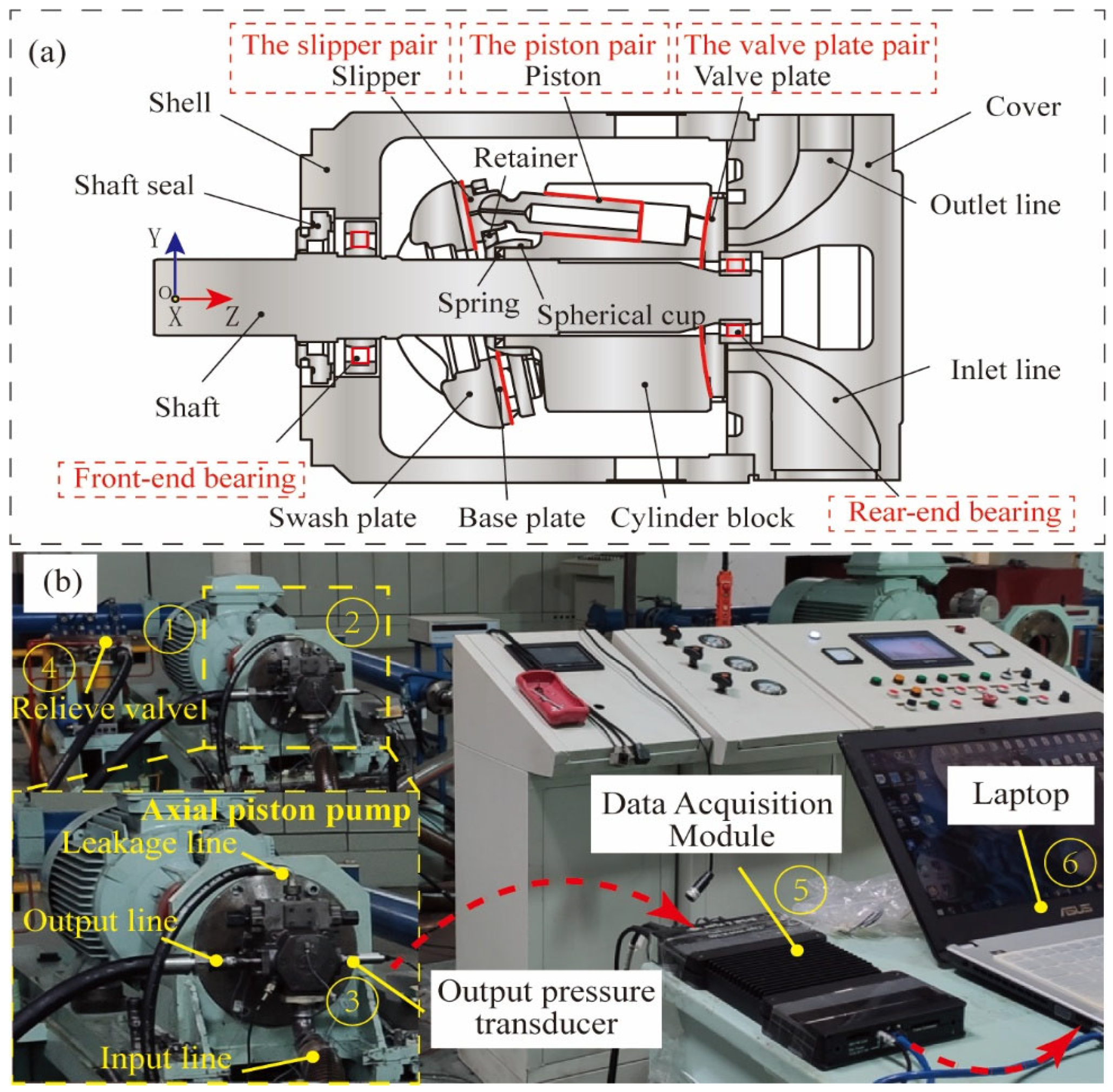
The intelligent diagnosis system for the axial piston pump can be broadly categorized into three key steps. In the primary stage, data acquisition equipment and monitoring software are employed to capture the pressure signals of the axial piston pump. Subsequently, a subset of training and testing samples can be randomly selected for analysis. In the second stage, the training sample subset is used to learn the GIN-ST model. Finally, in the third stage, a subset of test samples is inputted into the trained GIN-ST to obtain recognition outcomes for various fault modes.

5.1. Input Data

For future deployment of diagnostic models in the failure diagnosis of axial piston pumps, the present study avoids the use of traditional diagnostic models to extract deep-level features or multi-feature fusion approaches for input data. Instead, pressure signal data are collected from axial piston pump outlets and then normalized by means of minimum–maximum normalization [24]. Following this, an original signal is truncated using a sliding window of length 1024 without overlapping. After data segmentation, 2000 subsamples were generated for each dataset, of which the training set constituted 80%, with the remaining 20% retained for the test set. Subsequently, utilizing the weighted graph construction method proposed in Section 3.3 the graph data were constructed using subsamples taken from both the training set and the test set.

To further evaluate the intra-class variability of the dataset, we conducted a statistical analysis on key signal features extracted from samples within the same fault category. Specifically, we computed the standard deviation of root mean square (RMS), kurtosis, and spectral centroid across all samples in each fault class. The results reveal notable intra-class variation, particularly in the RMS and frequency domain features, which may be attributed to operating condition fluctuations and minor inconsistencies in fault progression.

Construction of the weight graph generates graph data for every 10 subsamples employed. Therefore, the resultant training set includes 160 subgraphs, and the test set comprises 40 subgraphs. Furthermore, the study considers two input types—the real-time domain (TD) input and frequency domain (FD) input, with the latter meaning preprocessing of subsamples through FFT.

5.2. Parameter Setting and Diagnostic Details

The experiment was conducted on a NVIDIA GeForce GTX 3080 Ti GPU, The software versions used for data processing in this text are Python version 3.8.6 and MATLAB version R2024b.The GIN-AM model $f$ is trained using a supervised end-to-end approach with loss $L=L_{cros}+\lambda {\mathcal{L}}_{ortho }$, where the cross-entropy loss is $L_{cros}$ and $\lambda$ is the proportion coefficient of orthogonal regularization. The number of layers $K=4$ is set, embedding dimension $D=64$, and regularization coefficient $\lambda =1.0\times {10}^{-5}$. Hyperparameters are adjusted by trial and error, with a batch size of 64, and with specific settings shown in the

Table 5. Experimental parameters.

Hyperparameters	Value
batch size	64
initial learning rate	0.0001
optimizer	Adam
edge weighting	Gaussian kernel
momentum	$1.0\times {10}^{-5}$
aggregation hidden size	128

.

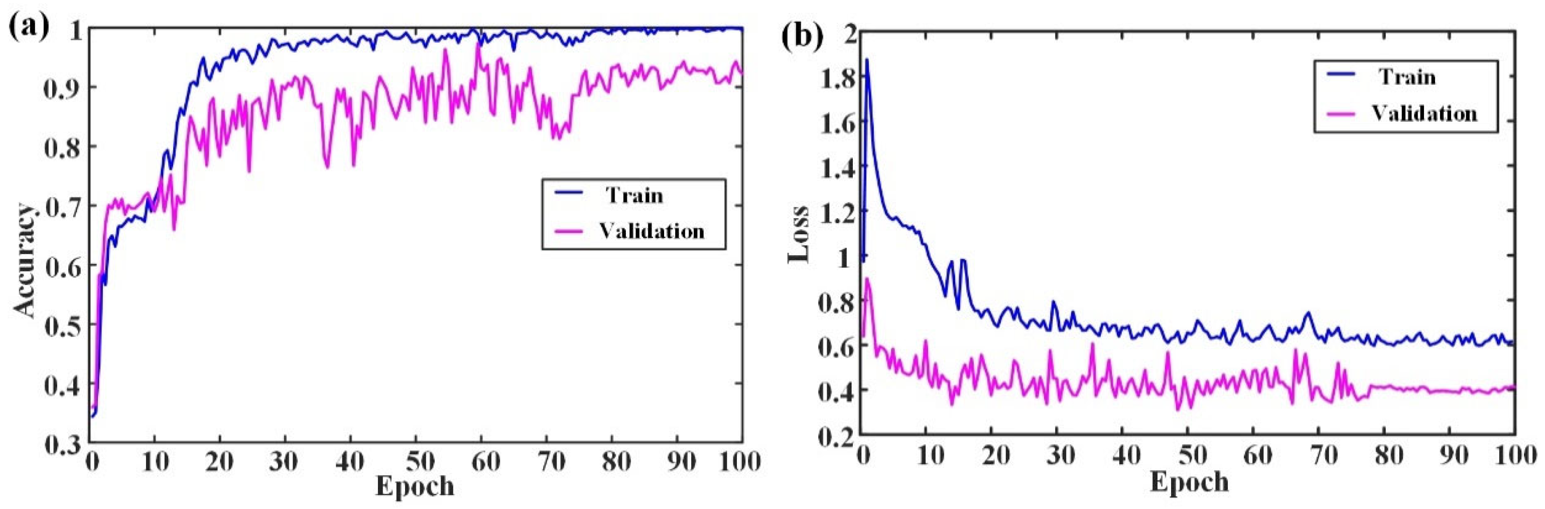
Figure 10 illustrates the training and validation process of the suggested fault diagnosis methodology for an axial piston pump on the GIN-ST model. To eliminate any potential random effects, five trails are conducted. The results in Figure 10 demonstrate that the GIN-ST model achieved convergence at epoch 100 with a training and validation loss approaching zero.

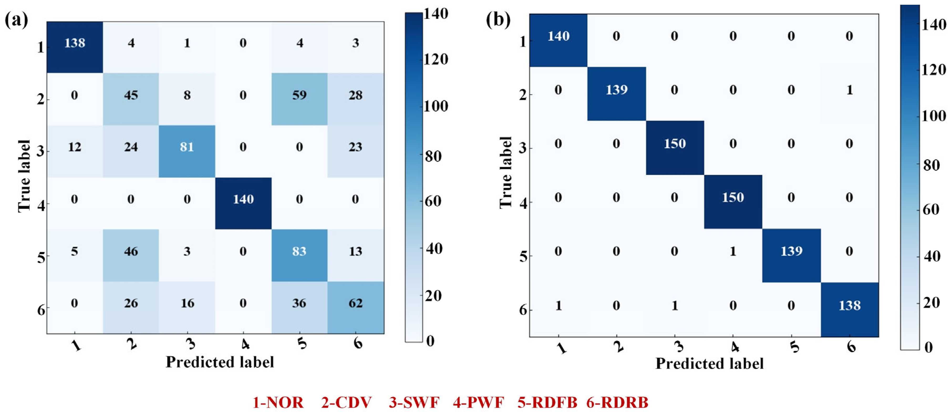
The confusion matrices in Figure 11 illustrate the performance of the proposed diagnostic method under both time domain and frequency domain input conditions. Within the graph, frequency domain input signifies the preprocessing of subsamples through the utilization of fast Fourier transform (FFT), aiding in the mitigation of noise interference inherent in time domain signals. 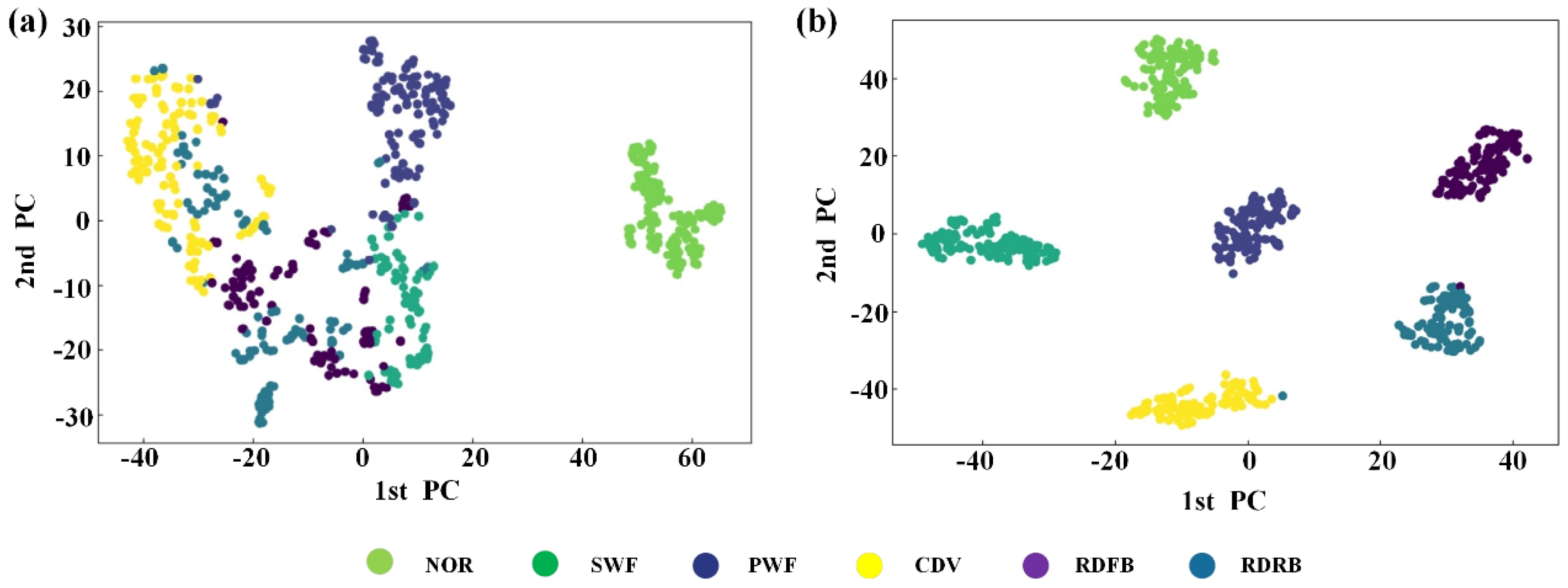The application of the proposed method to fault classification with two distinct inputs yields results as depicted in Figure 12a,b, respectively. The classification results show that predictions based on frequency domain input are markedly superior to those based on time domain input. This difference in outcome can be attributed to the substantial levels of noise present within the industrial working environment of axial piston pump systems. The application of FFT processing to the data can effectively reduce the disruptive influence of environmental noise on node features of the graph, thus enabling an easier acquisition of more meaningful node and graph representations.

To examine the outcomes of graph-based feature learning derived from the proposed model, we employed the widely utilized t-distribution stochastic neighbor embedding (t-SNE) method. The horizontal and vertical axes correspond to the two dimensions of the t-SNE embedding space, denoted as Component 1 and Component 2, respectively. As depicted in Figure 12, the t-SNE results reveal that in the time domain (TD), apart from capturing the typical characteristics of the plunger pump, the features associated with other fault categories exhibit incorrect classification. Conversely, in the frequency domain (FD), nearly all fault categories can be accurately classified.

5.3. Compared with Other Methods

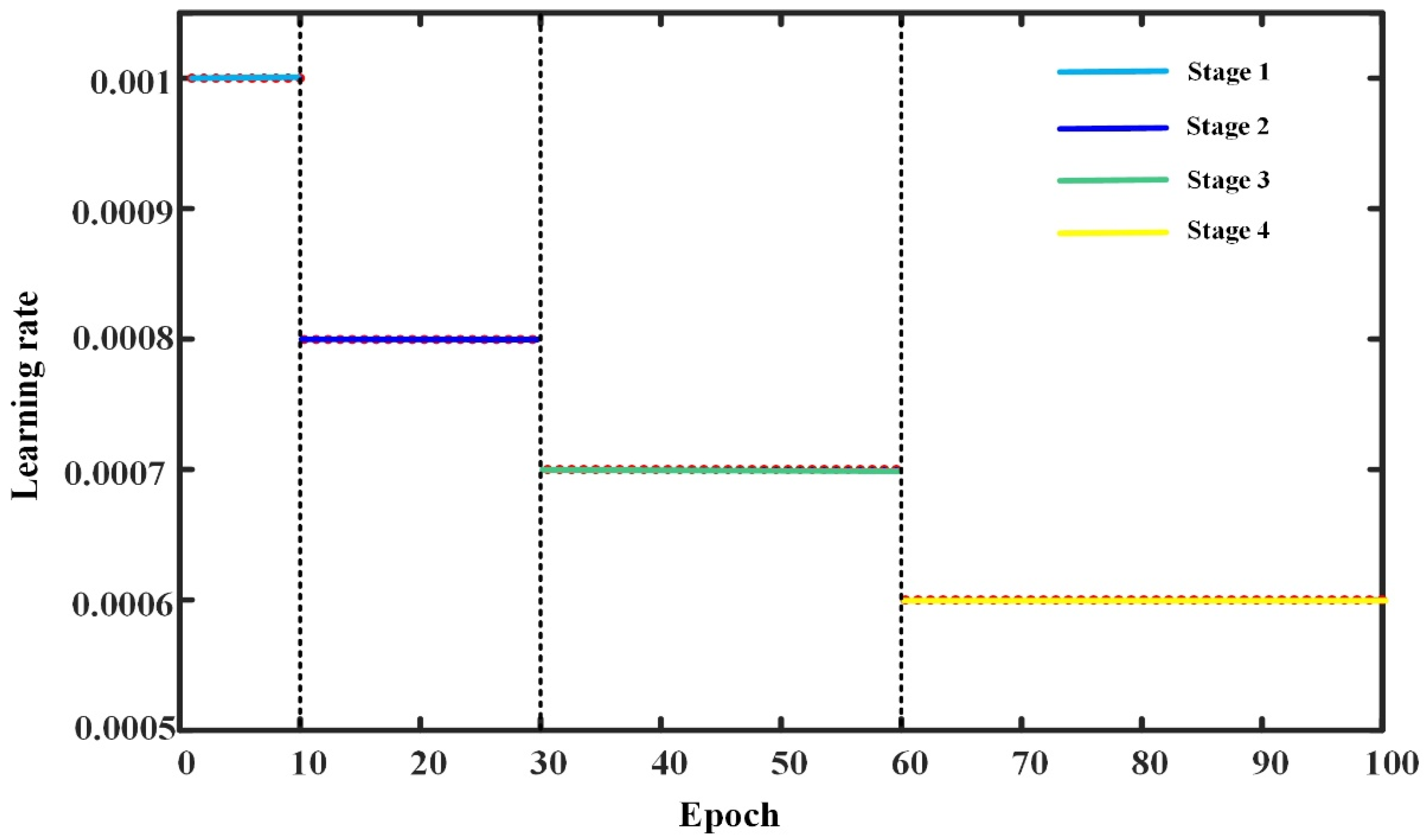
To demonstrate the efficacy and superiority of our proposed diagnostic approach, it is essential to compare it with other intelligent fault diagnosis methods. Accordingly, we benchmarked our GIN-ST algorithm against ARGCN [25], DCA-BiGRU [24], GCN [26], GAT [27], GIN [28], and other similar algorithms. Moreover, we compared our proposed method against the traditional five-layer CNN [23]. During our experimental process, the labeled samples were utilized before constructing the weighted graph as the input of CNN, while the weighted graph was used as the input of GCN. All models underwent training using 100 epochs with an initial learning rate of 0.001, and the learning rate during the model training process was adjusted through a multi-step strategy, which was divided into four stages: 0–10, 10–30, 30–60, and 60–100 training epochs, each using a different learning rate. The specific setting strategy is shown in Figure 13 and the optimizer was set to Adam.

To mitigate potential impacts of random events on our findings and to underscore the robustness and dependability of our proposed methodology, five experiments were performed. The assessment of classification efficacy centered on the overall classification accuracy, encompassing metrics such as maximum accuracy (max-acc), minimum accuracy (min-acc), average accuracy (avg-acc) across five trials, and training duration. The classification outcomes of various methods are delineated in

Table 6. Failure diagnosis results of axial piston pumps using different methods.

Models	Max-acc (%)	Min-acc (%)	Avg-acc (%)	Time (s)
CNN	93.83	90.94	$92.81 \pm 1.19$	119
ARGCN	91.36	86.88	$89.35 \pm$1.38	101.8
DCA-BiGRU	94.82	92.64	$93.94 \pm 0.87$	182.6
GCN	90.61	86.92	$89.27 \pm 1.41$	93.4
GAT	94.06	91.86	$93.09 \pm 0.84$	94.1
GIN	96.72	93.69	$95.2 \pm 1.24$	98.5
GIN-ST	98.8	96.06	$\mathbf{97.31}\mathbf{\pm }\mathbf{0.40}$	105.2

.

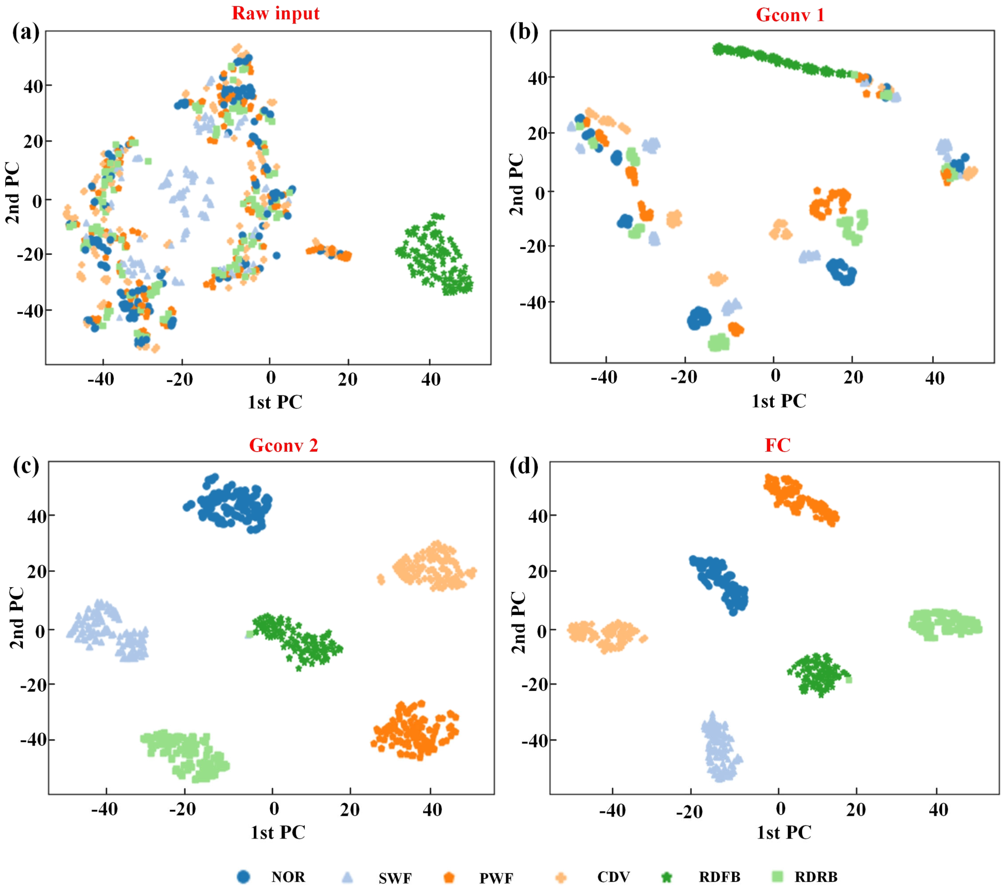
The failure diagnosis model presented in this study learns the process of graph feature in each layer, as demonstrated in Figure 14. The graph depicts scattered points in the distribution of features of the raw input. However, certain features in the RDFB category () tend to cluster; meanwhile, the majority of features representing other category faults continue to display almost uniform distribution, even after being processed by GConv1. Further information extraction by GConv2 enables the classification and clustering of distinct faults features. Eventually, feature clustering is established in the same type through the learning of FC, and clear classes are distinguishable at this stage. By utilizing the frequency domain input of the pressure signals, GIN-AM successfully accomplishes fault classification of the axial piston pump.

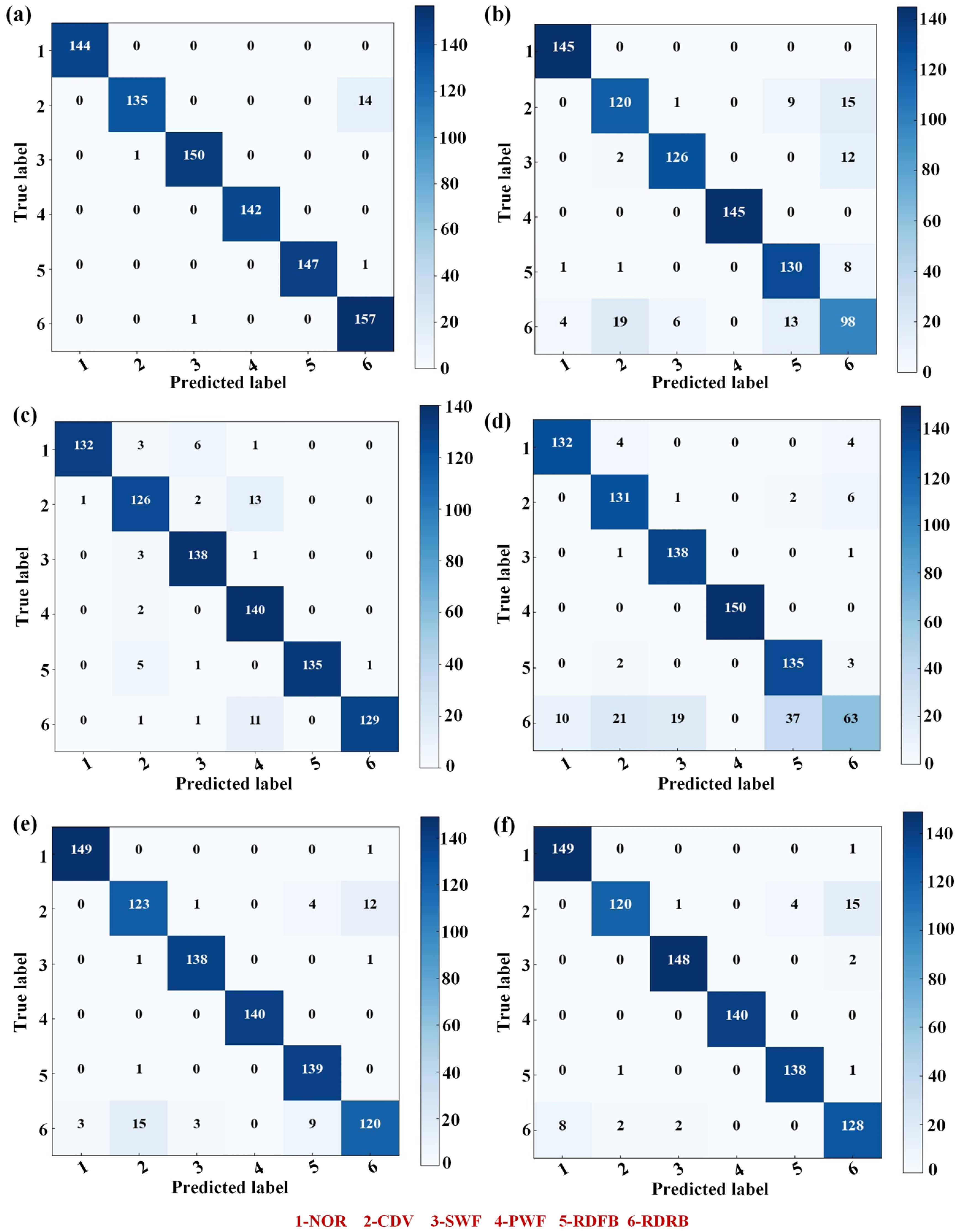
Figure 15 illustrates the confusion matrices of various intelligent failure diagnosis methods, excluding the proposed approach, under a similar frequency domain input. The classification results indicate substantial inconsistencies in sensitivity to strong noise among different diagnosis model input features. Moreover, it is commonly observed that graph convolutional neural networks with an attention mechanism (GAT) and GIN show significant superiority over other methods. Therefore, this paper provides an idea for designing a spatio-temporal attention mechanism module based on the traditional GIN model.

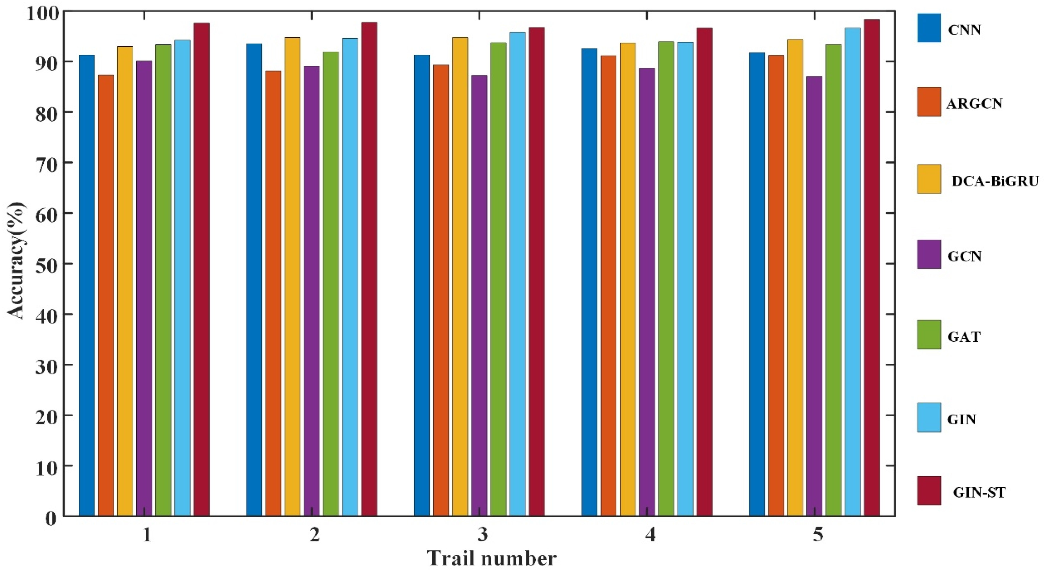
Further, the diagnostic results of the above six intelligent fault diagnosis methods in five random trails were compared with the proposed GIN-ST, as shown in Figure 16. The performance of GIN-ST is noted for its remarkable stability, consistently achieving peak performance across all datasets. The average diagnostic accuracies of GIN-ST for each dataset are 97.59%, 97.75%, 96.70%, 96.62%, and 98.28%, respectively. These figures underscore that the proposed method delivers the most comprehensive and optimal results in terms of efficiency and accuracy, particularly under conditions of significant noise interference.

To enhance the complexity of fault diagnosis, white noise with varying signal-to-noise ratios (SNR) was introduced into the dataset, mimicking the noise found in various operating conditions of axial piston pumps. Subsequently, the resulting dataset was randomly divided into a training set (80%) and a testing set (20%). Illustrated in Figure 17, the diagnostic accuracies of the aforementioned methods were assessed under different levels of random noise. The classification results demonstrate the superior noise resistance performance of the GIN-ST model compared to other fault diagnosis methods, primarily attributed to the design of the spatio-temporal attention module, which emphasizes fault features. Thus, these experimental findings indicate that the proposed model shows enhanced robust stability and noise resistance performance for diagnosing variable working conditions in axial piston pumps.

5.4. Ablation Research

In this section, two variants of the GIN-ST model are proposed for the ablation study that are aimed at evaluating the individual impact of model components on the final prediction outcomes: (1) UWG-GIN-ST, which transforms subsamples of the original signal into unweighted graphs as inputs for GIN-ST, wherein the importance of node neighbors is considered equally important. (2) WG-GIN, which omits the design of spatio-temporal dynamic attention mechanisms, employing the original GIN network with inputs as subsamples of the original signal transformed into weighted graphs but without the designed attention-based READOUT module and Transformer encoder. The average accuracy of both model variants in diagnosing faults in the axial piston pump over five instances is presented in

Table 7. Results of ablation study on fault diagnosis.

Methods	UWG-GIN-ST	WG-GIN	GIN-ST
Trail 1	92.05	90.82	97.59
Trail 2	93.81	89.3	97.75
Trail 3	92.64	89.14	96.70
Trail 4	93.2	91.76	96.62
Trail 5	90.44	88.54	98.28
Aver (%)	92.26 ± 1.11	89.91 ± 1.33	97.39 ± 0.71

.

The analysis results in Table 7 indicate that the average predictive accuracy of the proposed GIN-ST is 5.13% higher than that of UWG-GIN-ST. This suggests that weighted graphs should be used as inputs during the graph convolution operation, acknowledging the varying importance of node neighbors. Furthermore, GIN-ST outperforms WG-GIN by 7.48%, demonstrating that the introduction of a novel attention-based READOUT module and Transformer encoder effectively addresses the issue of incorporating temporal information into input node features. This approach facilitates the connection of encoded timestamps with node features, enabling the decoding of deeper global features associated with various faults in the axial piston pump. Consequently, this enhances fault classification accuracy.

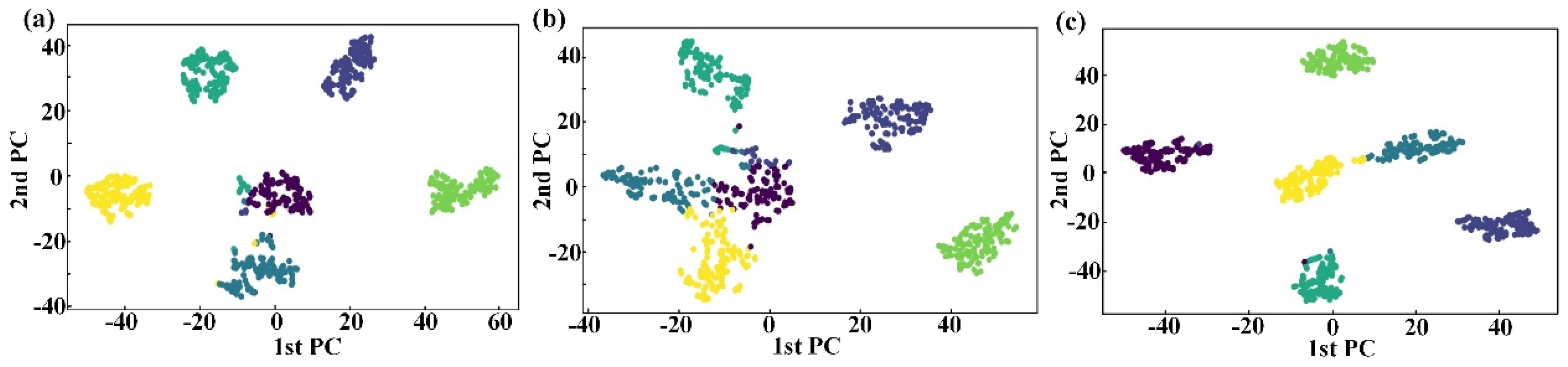
To showcase the efficacy of these three models in feature learning, the features extracted from the last layer of the feature extractor are visualized through T-SNE. Figure 18 shows the visualization features of these three different models to illustrate their impact on the task.

From the feature visualization and classification results in Figure 18a, b, it is evident that both UWG-GIN-ST and WG-GIN struggle to effectively distinguish between the rolling element damage of the front-end bearing (RDFB, ) and rolling element damage of the rear-end bearing (RDRB, ). This observation suggests that employing unweighted graphs as the input and omitting the spatiotemporal dynamic attention module are detrimental to the accurate classification of fault features in the axial piston pump. The feature visualization and classification results of the proposed method, as shown in Figure 18c, demonstrate that the proposed approach successfully and comparatively accurately classifies various fault features.

5.5. Real-Time Feasibility

To assess the applicability of the proposed method in embedded or on-board monitoring scenarios such as aircraft or railway systems, we evaluated its real-time feasibility in terms of computational latency and resource demand. The model was deployed on a representative edge computing platform (e.g., NVIDIA Jetson Nano with 4 GB RAM and quad-core ARM CPU), and inference time was measured using preprocessed input signals of fixed length (e.g., 1024 points after FFT).

The average inference time per sample was approximately 22.6 ms, which meets the real-time processing requirement for most low-frequency hydraulic monitoring tasks. Compared with a baseline 1D CNN, our GNN-based model demonstrated slightly higher latency (by ~6 ms) but provided significantly improved accuracy and noise robustness. The memory footprint remained below 250 MB during inference, ensuring compatibility with embedded environments.

6. Conclusions

In this paper, the GIN-ST model is introduced, presenting a novel fault diagnosis framework derived from the traditional GIN model by incorporating a spatio-temporal attention mechanism. The proposed method is applied to fault diagnosis in axial piston pumps under conditions of significant noise interference. Empirical results validate that GIN-ST surpasses other intelligent diagnostic tools in both classification accuracy and robustness. The following summarizes the conclusions drawn from this study:

(1)

A novel attention-based READOUT module and Transformer encoder was developed which can decode the deeper whole graph features of different faults in an axial piston pump. The proposed model can enhance the performance of the classification task and offers spatio-temporal interpretability.

(2)

This study investigated the effect of different inputs on fault diagnosis models and found that frequency domain input can partially mitigate the impact of strong noise on fault graph node features. However, diagnostic methods varied in sensitivity to noise. By introducing a spatio-temporal attention mechanism into the diagnostic model, the fault diagnosis of axial piston pumps under strong noise conditions can be more robust.

(3)

After comprehensive consideration of efficiency and accuracy, as well as a comparison of predictive results with other intelligent fault diagnosis methods, it was determined that GIN-ST exhibits superior diagnostic accuracy and robustness in the diagnosis of piston pump faults, particularly under conditions of strong noise.

Furthermore, the proposed method shows strong potential for integration into on-board aircraft health monitoring systems (AHMS). Its lightweight architecture, robustness to noise, and ability to extract discriminative features from non-stationary signals make it suitable for real-time condition monitoring under the strict operational and safety requirements of aviation environments.

In future work, we plan to explore hybrid modeling approaches that integrate physics-informed knowledge with data-driven representations. Specifically, incorporating fluid mechanics models—such as leakage flow equations, pressure drop formulations, and volumetric efficiency constraints—can provide a physically consistent foundation to augment the learned features from the GNN framework. This fusion of domain knowledge and deep learning has the potential to improve interpretability, enhance generalization to unseen fault modes, and enable failure diagnosis under sparse data conditions. Such hybrid architectures are particularly promising for safety-critical applications such as aviation hydraulics, where explainability and reliability are essential.