Analytic Continual Learning-Based Non-Intrusive Load Monitoring Adaptive to Diverse New Appliances

Abstract

Non-intrusive load monitoring (NILM) provides a cost-effective solution for smart services across numerous appliances by inferring appliance-level information from mains electrical measurements. With the rapid growth in appliance diversity, continual learning that adapts to new appliances while retaining knowledge of previously learned appliances is of great interest. However, existing methods can handle only a few new appliance types and suffer from high computational complexity and data leakage risks. Therefore, an analytic continual learning-based (ACL) NILM method is proposed. The method employs a lightweight model that is constructed with dual output branches using depthwise separable convolution for load identification and novelty detection. Meanwhile, a supervised contrastive learning strategy is applied to enhance the distinctiveness among appliance types in the feature extraction module. When the novelty detection branch determines that new data need to be learned, the parameters of the dual branches are updated by recursively calculating the analytical solution using only the current data. Experiments on four public datasets demonstrate superior performance on pre-collected appliances with lower computational effort. It also significantly outperforms existing methods during the continual learning process, as the number of appliance types increases to 56. The practicality of the proposed method is validated through a real-world application on an STM32F407-based smart socket.

1. Introduction

The smart grid integrates power transmission with information flows, offering the possibility of better electricity usage. However, limited access to appliance-level data renders behind-the-meter electricity usage at the grid’s edges a “black box”. Therefore, non-intrusive load monitoring (NILM), which estimates the operation of appliances only by analyzing mains electrical measurements, has emerged as a major research focus. It eliminates the need for installing separate sensors for each appliance, offering a cost-effective way to obtain fine-grained data [1]. Appliance-level data enable grid operators to design personalized demand–response programs tailored to users’ electricity usage patterns. At the same time, it brings direct benefits to users through services such as appliance maintenance, smart homes, and energy management [2].

NILM is categorized into two pathways: event-less and event-based. The former directly decomposes long-term aggregated power consumption into target appliance usage [3]. The latter first detects the leap of mains’ measurements in real time, extracts the corresponding event waveforms, and then estimates the appliance types using a load identification model [4]. The event-based pathway is prioritized due to the following three inherent advantages: (1) It is more suitable for monitoring multiple appliances in a single-load identification model, aligning with the growing diversity of appliances. (2) By focusing on appliance-specific characteristics, identification models designed for single-event waveforms are more robust to external factors such as user behavior. (3) Benefiting from high-frequency sampling, it has a wider range of application scenarios due to its faster response.

Although there are many event-based NILM studies, they focus on improving the learning of appliances in pre-collected datasets. However, rapid economic growth and technological advances have led to rich appliance diversity, making it impractical to collect data on all appliances in advance [5]. Therefore, in real-world applications where new users join or when monitoring requirements evolve, NILM models must continually update their parameters to adapt to emerging appliances in streaming data. Crucially, the integration of new appliance types does not negate the need to maintain the identification abilities for existing appliances. This necessitates preserving learned waveform-to-type mapping relationships during streaming data adaptation to mitigate catastrophic forgetting, a phenomenon where acquiring new knowledge degrades performance on original appliances [6]. While existing NILM methods based on transfer learning or meta-learning leverage accumulated knowledge to accelerate adaptation to new appliances [4,7,8], these methods exhibit critical limitations in streaming data contexts. Specifically, they are designed for single-round parameter updates using pre-collected target appliance datasets, inherently disregarding the retention of historical knowledge during learning. As a result, the continual learning paradigm for streaming data is attracting growing attention [9]. This paradigm aims to continually improve the identification of new appliances while preserving knowledge of previously learned ones.

Current continual learning methods in NILM aim to mitigate catastrophic forgetting by jointly training new data and original data. Pioneering work [10] introduced continual learning into NILM. When new data arrive, this method first evaluates performance to determine whether to randomly select stored data for joint fine-tuning. It then updates the appliance library based on waveform similarity. Ref. [11] employs density-based spatial clustering of applications with noise (DBSCAN) to extract representative waveforms when updating the appliance library, thereby reducing the forgetting of important knowledge more effectively. Ref. [12] selects important waveforms for storage using attention weights from the NILM model, but it is limited to specific model architectures. To avoid storing original appliance data, Ref. [13] leverages a generative model to recreate waveforms for joint fine-tuning with new data. But, the generative model may provide a biased representation of the original data and is difficult to update continually in streaming data. Moreover, ref. [14] applies a knowledge distillation loss on the original data during fine-tuning and scales the model’s output layer according to the parameter ratios of new and original appliance types to mitigate forgetting. Ref. [15] further selects model layers for dynamically updating based on the loss, but this significantly increases the complexity of continual learning. However, all existing continual learning-based NILM methods rely on storing substantial original data or generators, which not only burdens computational resources but also raises the risk of sensitive appliance data leakage. Furthermore, despite storing original data, the monitoring performance of existing methods still degrades rapidly as more new appliances are added.

Before the continual learning of load identification models, it is also necessary to detect whether the incoming data contain new appliances, which is known as novelty detection. In real-world scenarios, streaming data often include both new and previously seen appliances. Novelty detection helps prevent unnecessary model updates. It also prevents new appliance types from being identified as existing types in event-based NILM. Existing novelty detection methods focus on similarity matching using either raw waveforms or extracted features. Ref. [16] designs complex matching rules based on dynamic time warping, but they are limited to low-frequency power data and are sensitive to noise. Ref. [17,18] transform appliance waveforms into images, which are then matched in feature space using Euclidean distance. In contrast, ref. [19] uses DBSCAN to adaptively detect new data based on density in the feature space, avoiding manual tuning of distance thresholds. To enhance the flexibility of similarity computation, Ref. [20] uses a neural network in the feature space of the Siamese network to compute pairwise similarity. However, these methods are not only inefficient in similarity matching but also rely on storing large amounts of original data, facing the same critical challenges as continual learning-based load identification methods in streaming data. Moreover, these novelty detection methods are not yet capable of continual learning. As the NILM model learns new appliances, the novelty detection method must also be updated to prevent misclassifying previously learned appliances as new in subsequent streaming data.

To handle new appliances in streaming data while avoiding the complexity and data leakage risks of data storage, an analytic continual learning-based NILM method is proposed. To the best of our knowledge, this is the first NILM method that eliminates dependency on original data during continual learning while providing theoretical robustness against catastrophic forgetting. The contributions of this paper are summarized as follows:

(1)

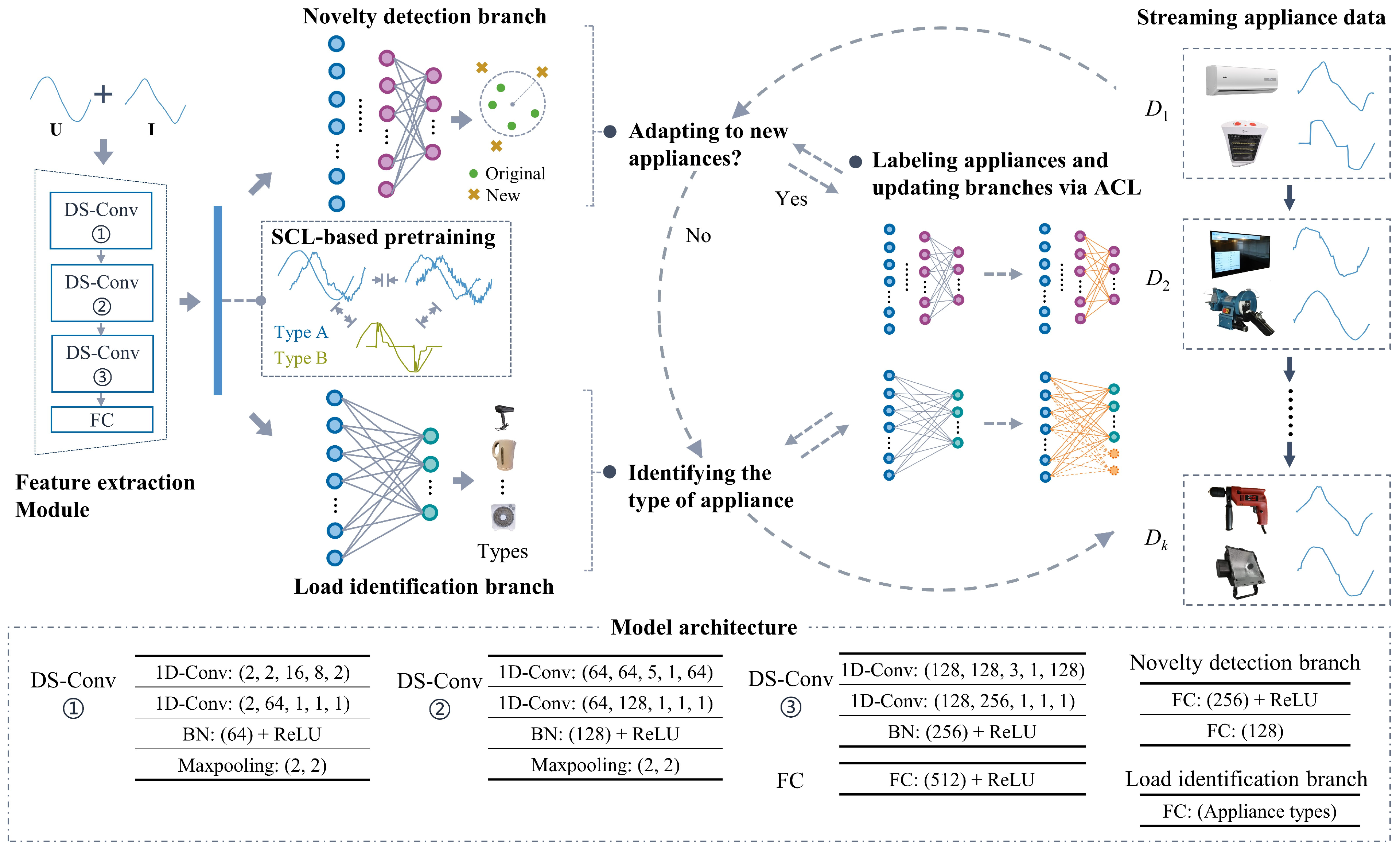
An analytic, continual learning-based framework adaptive to diverse new appliances is proposed. This framework establishes a closed-loop iteration between novelty detection and continual learning for streaming appliance data. It eliminates original data storage requirements and learns new appliances through a single forward propagation.

(2)

A unified model is designed featuring a depthwise separable convolutional feature extractor and dual output branches for load identification and novelty detection. Crucially, the novelty detection branch represents the original data via a hypersphere center and radius in feature space, avoiding the need for data storage.

(3)

A supervised contrastive learning-based pretraining strategy is proposed to enhance intra-type clustering and inter-type separation in feature space. This strategy provides a strong foundation for analytic, continual learning, enhancing both learning efficiency and task performance of load identification and novelty detection.

(4)

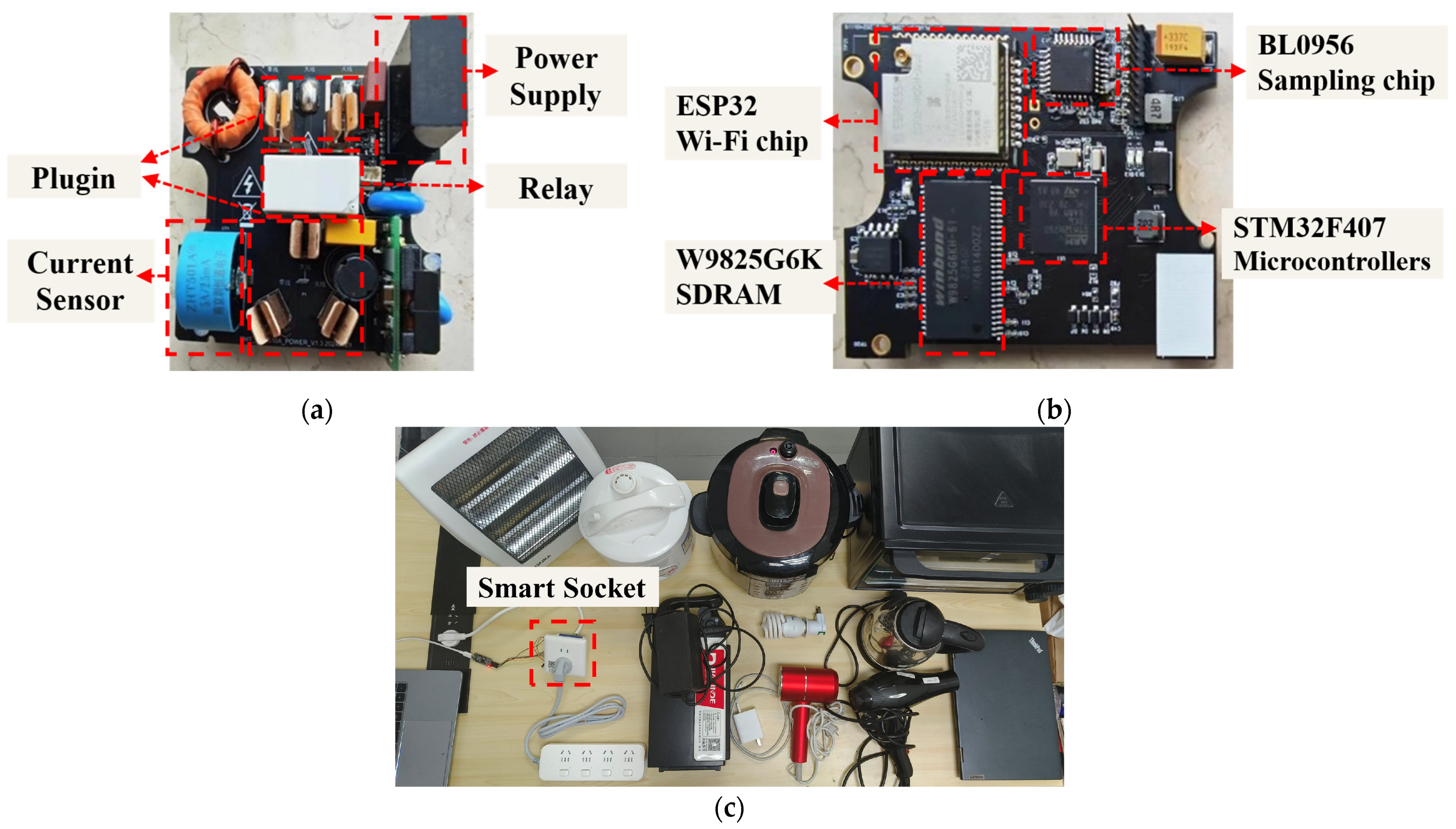
Extensive experiments are conducted on four public datasets covering 56 appliance types. The results demonstrate that the proposed method significantly outperforms existing continual learning-based NILM methods. Additionally, deployment testing on an STM32F407-based smart socket confirms the viability of the proposed method in real-world settings.

2. Problem Statement

2.1. Event-Based NILM

Event-based NILM involves three steps: event detection, waveform extraction, and load identification. First, the timing of appliance state changes is detected by comparing sequence differences within a sliding window [4]. Next, the current sequences I^b and I^a and voltage sequences U^b and U^a, before and after the event, are selected. Based on Kirchhoff’s law, the appliance current waveform I^e = I^a − I^b and the voltage waveform as U^e = (U^b + U^a)/2 corresponding to this event are extracted. Finally, the load identification model fⁱ(I^e, U^e; Wⁱ), parameterized by Wⁱ, maps the event waveforms to appliance types. Specifically, Wⁱ is typically learned via gradient descent on the collected dataset D₀ ~ {$I_0^{\mathrm{e}}$, $U_0^{\mathrm{e}}$, Y₀}, where Y₀ denotes the corresponding appliance types.

2.2. The Continual Learning Setting of NILM

In real-world applications, NILM models need to not only perform well on test data from the collected dataset D₀ but also continually learn from streaming data to adapt to new appliances. Streaming data are represented as a sequence of appliance datasets, {D₁ ~ {$I_1^{\mathrm{e}}$, $U_1^{\mathrm{e}}$, Y₁}, …, D_k ~ {$I_k^{\mathrm{e}}$, $U_k^{\mathrm{e}}$, Y_k}}, arriving in temporal order, with k denoting the number of data increment rounds [10]. In particular, the diversity of appliances causes variations in waveform distributions across datasets and differences in the appliance types of Y_k. Therefore, when new data arrive, a novelty detection model fⁿ(I^e, U^e; Wⁿ), parameterized by Wⁿ, is required to determine whether the appliances are already learned. If unknown appliances are detected, their types also need to be labeled. In the subsequent continual learning process, the NILM model should try to retain its original ability after updating its parameters on new data. For the load identification model, updating $W_{k-1}^{\mathrm{i}}$ to $W_k^{\mathrm{i}}$ extends its scope from identifying appliances in D₀ ~ D_k−1 to those in D_k. For the novelty detection model, updating $W_{k-2}^{\mathrm{n}}$ to $W_{k-1}^{\mathrm{n}}$ incorporates appliances in D_k−1 into the learned set, alongside those in D₀ ~ D_k−2, while continuing to treat appliances in D_k as novel.

3. Methodology

3.1. NILM Framework for Adapting to Diverse New Appliances

The proposed framework is shown in Figure 1. As the preparation for continual learning, a lightweight model with dual output branches is first built using depthwise separable convolutions, as shown in the left part of Figure 1. In the model, the feature extraction module transforms appliance waveforms into informative features. The load identification branch maps the features to appliance types. The novelty detection branch encloses the original data by constructing hyperspheres in the feature space. To enhance the feature representation and facilitate adaptation to new appliances, a pretraining strategy based on supervised contrastive learning (SCL) is proposed, as shown in the middle of Figure 1. When applied to streaming appliance data, the model first freezes all parameters except for the output layers. It then iteratively performs novelty detection and continual learning, as shown in the right part of Figure 1. When new data arrive, the novelty detection branch first determines whether the appliances are learned. If so, the appliance types are estimated by the load identification branch. If not, the appliance types of the unknown waveforms need to be labeled, and continual learning is then triggered. During continual learning, the load identification branch first expands its output layer according to the number of appliance types. Then, the parameters of the two output branches are recursively updated through analytic continual learning: on the one hand, data from new appliances are integrated into the waveform-to-type mapping of the original appliances; on the other hand, features of the new appliances are adjusted within the original hypersphere.

3.2. Lightweight Dual-Branch NILM Model

The proposed model consists of a feature extraction module, a novelty detection branch, and a load identification branch. Its detailed architecture is shown in the lower part of Figure 1. Given the close relevance between novelty detection and load identification, the dual branches share a common feature extraction module for improved computational efficiency. The model takes current and voltage waveforms concatenated along the channel dimension as input. These simple inputs preserve key electrical characteristics and their temporal dependencies. The feature extraction module comprises three stacked submodules followed by a fully connected layer. Each submodule sequentially connects depthwise separable convolution, batch normalization, and a ReLU activation function. Specifically, the depthwise separable convolution decomposes a standard convolution into a depthwise one-dimensional (1D) convolution within each channel and a pointwise 1D convolution that aggregates information across channels. This design significantly reduces computational costs [21]. Batch normalization standardizes each feature in a training batch using its mean and variance [22]. Its learnable parameters enable the model to adapt to the amplitude distribution of diverse appliance waveforms. Notably, the proposed model is more lightweight in both input and architecture than the existing NILM models based on image-based waveform representations and two-dimensional convolution networks (2D-CNNs) [5,23]. This lightweight design is motivated by the following reasons: (1) It enables easy deployment on low-resource hardware, especially when continual learning from streaming data is required. (2) Using raw waveforms as input reduces data processing complexity and minimizes the parameter count of the feature extraction module. (3) The lightweight 1D convolution has been proven effective in extracting features from appliance waveforms [4].

To avoid storing original appliance data, the novelty detection branch adopts the deep support vector data description (SVDD) method [24]. Specifically, two fully connected layers map the discriminative feature X^en, produced by the feature extraction module, to a feature space where learned appliances are tightly clustered. Since only data from learned appliances are available when constructing the mapping f(X^en; Wⁿ), the objective is to enclose these data points as tightly as possible within a hypersphere centered at c with radius r, as shown in (1). The hypersphere center c is set to the initial mean of the original appliance data in the feature space. In this space, the 99th percentile of distances from the center is used as a detection threshold. A feature exceeding this threshold is detected as a new appliance. To prevent trivial minimization of (1) by setting Wⁿ to zero, the fully connected layers in the novelty detection branch are implemented without bias terms.

$${\displaystyle \underset{W^{\mathrm{n}}}{\min }}{\displaystyle \frac{1}{m}}{\displaystyle \sum _{j=1}^m{‖f(X_j^{\mathrm{e}\mathrm{n}};W^{\mathrm{n}})-c‖}_2}+\lambda {‖W^{\mathrm{n}}‖}_2$$

(1)

3.3. Supervised Contrastive Learning-Based Pretraining Strategy

The pretraining on the initial dataset D₀ provides the foundation for continual learning and determines the upper bound of NILM performance on subsequent streaming data. The proposed pretraining strategy consists of two stages. First, the feature extraction module is trained jointly with the load identification branch. Then, the novelty detection branch is trained separately. This separation is necessary because the load identification branch learns to distinguish among original appliance types, while the novelty detection branch learns to treat them as a single group. This conflict has limited impact, as more discriminative features reduce the risk of confusing new appliances with original ones. In addition, the novelty branch includes one extra fully connected layer compared to the load identification branch, facilitating the transformation between the two kinds of feature spaces.

In the pretraining stage, in addition to the cross-entropy loss in existing continual learning-based NILM methods, a SCL-based loss [25] is applied to the feature extraction module parameters W^en, as shown below:

$${\displaystyle \underset{W^{\mathrm{en}}}{\min }}{\displaystyle {\displaystyle \sum _{j\in I}}\frac{-1}{\left|L(j)\right|}{\displaystyle {\displaystyle \sum _{l\in L(j)}}\log \frac{\exp (X_j^{\mathrm{en}}\cdot X_l^{\mathrm{en}}/\tau )}{{\displaystyle {\displaystyle \sum _{a\in I\backslash \left\{j\right\}}}\exp (X_j^{\mathrm{en}}\cdot X_a^{\mathrm{en}}/\tau )}}}}$$

(2)

where I denotes the set of sample indexes in a training batch, L(j) is the set of indexes sharing the same appliance type as the jth sample (excluding j itself), and τ is the temperature parameter used in the dot-product similarity calculation.

Compared to the unsupervised contrast learning loss that is commonly used in NILM, which only improves inter-sample distinctiveness [19,26], the SCL-based loss leverages label information to enhance inter-type separation and intra-type clustering, as shown in the middle part of Figure 1. This reduces the learning difficulty for both the novelty detection and load identification branches. To facilitate the SCL to better distinguish different types of features, the waveforms are augmented by adding random Gaussian noise I^g and random wandering noise I^r [27], doubling the training set. In particular, Gaussian noise simulates typical background noise, while random wandering noise models the variations in appliance waveforms. Both types are applied in equal proportion. For the first time, random walk noise is introduced as an augmentation method that is specifically adapted to NILM. This approach better reflects the electrical characteristics of appliances, enabling augmented samples to retain key distinctive features while more accurately representing the variations within the same appliance type. As shown in Figure 2, even with the same signal-to-noise ratio (SNR) of 5 dB, random walk noise preserves the flat peaks of air conditioner waveforms and the plateau in Halogen Fluter waveforms. These noise sequences are derived from unit noise I^g′ and I^r′, scaled according to the preset SNR and the signal power P^w of the appliance waveform, as shown in (3)~(5).

$$I^{\mathrm{g}}=\sqrt{P^{\mathrm{n}}}\times I^{\mathrm{g}\prime }$$

(3)

$$I^{\mathrm{r}}=\sqrt{P^{\mathrm{n}}}\times I^{\mathrm{r}\prime }$$

(4)

$$P^{\mathrm{n}}={\displaystyle \frac{P^{\mathrm{w}}}{{10}^{SNR/10}}}$$

(5)

3.4. Analytic Continual Learning-Based NILM Model Updating Strategy

In streaming data, the NILM model needs to extend its novelty detection and load identification abilities from appliances in D₀~D_k−1 to those in D₀~D_k as D_k arrives. To avoid the complexity and potential data leakage associated with storing original data, only the latest D_k was used in each round of continual learning. Without access to previous data, capturing the correlations and distinctions between new and original appliances becomes more difficult, increasing the risk of catastrophic forgetting. Recently, analytic continual learning has emerged as a new branch of continual learning [28], with preliminary validation in autonomous driving [29] and hyperspectral classification [30]. The core of the method is recursive Moore–Penrose learning, which treats D₁ to D_k in streaming data as blocks in blockwise linear regression. It theoretically guarantees that learning D₀ to D_k sequentially is equivalent to learning them simultaneously, eliminating the need to store original data and preventing catastrophic forgetting. Benefiting from the strong representation ability of the feature space obtained through the pretraining strategy in Section 3.3, the linearity assumption required for analytic continual learning can be effectively approximated. Therefore, it is expected to enable NILM to adapt to diverse new appliances.

Once continual learning is triggered, the feature extraction module and the first fully connected layer in the novelty detection branch are frozen. For the load identification branch, if the new data contain new appliance types, the parameters $W_k^{\mathrm{i}}$ of the fully connected layer need to be extended to match the total number of types. Assuming the data from D₀ to D_k are stored, the optimal solution for $W_k^{\mathrm{i}}$ in joint training is as follows:

$$W_k^{\mathrm{i}\ast }={\displaystyle \underset{W_k^{\mathrm{i}}}{\arg \min }}({‖Y_{0~k}-X_{0~k}^{\mathrm{en}}{W}_k^{\mathrm{i}}‖}_{\mathrm{F}}^2+\gamma {‖W_k^{\mathrm{i}}‖}_{\mathrm{F}}^2)$$

(6)

where γ is the weight coefficient of the regularization term.

The above optimization problem has an analytic solution, as shown below:

$$W_k^{\mathrm{i}\ast }={({\displaystyle \sum _{j=0}^k{(X_j^{\mathrm{en}})}^{\mathrm{T}}{X}_j^{\mathrm{en}}}+\gamma I)}^{-1}({\displaystyle \sum _{j=0}^k{(X_j^{\mathrm{en}})}^{\mathrm{T}}{Y}_j})=R_k{Q}_k$$

(7)

According to the Woodbury matrix identity [31], R_k can be calculated recursively from D₀ to D_k, as shown in the following:

$$R_k={(R_{k-1}^{-1}+{(X_k^{\mathrm{en}})}^{\mathrm{T}}{X}_k^{\mathrm{en}})}^{-1}=R_{k-1}-R_{k-1}{(X_k^{\mathrm{en}})}^{\mathrm{T}}{(I+X_k^{\mathrm{en}}{R}_{k-1}{(X_k^{\mathrm{en}})}^{\mathrm{T}})}^{-1}{X}_k^{\mathrm{en}}{R}_{k-1}$$

(8)

Further, Q_k is expanded to obtain the following:

$$W_k^{\mathrm{i}\ast }=R_k{Q}_k=R_k{Q}_{k-1}+R_k{X}_k^{\mathrm{en}}{Y}_k$$

(9)

Substituting (8) into (9) yields the following:

$$R_k{Q}_{k-1}=(I-R_k{(X_k^{\mathrm{en}})}^{\mathrm{T}}{X}_k^{\mathrm{en}})W_{k-1}^{\mathrm{i}\ast }$$

(10)

Then, substituting (10) into (9) gives the recursive computation of $W_k^{\mathrm{i}\ast }$ from D₀ to D_k, as shown below:

$$W_k^{\mathrm{i}\ast }=(I-R_k{(X_k^{\mathrm{en}})}^{\mathrm{T}}{X}_k^{\mathrm{en}})W_{k-1}^{\mathrm{i}\ast }+R_k{(X_k^{\mathrm{en}})}^{\mathrm{T}}{Y}_k$$

(11)

Consequently, when the streaming appliance data D_k arrives, R_k is first calculated according to (8), followed by the recursive computation of $W_k^{\mathrm{i}\ast }$ using (11), eliminating the need to store data from D₀ to D_k−1. Notably, $W_0^{\mathrm{i}}$ can also be recalculated according to (7) after the pretraining process described in Section 3.3. This reduces the error introduced by gradient descent, bringing the result closer to the analytic optimal solution for D₀.

For continual learning in the novelty detection branch, $W_k^{\mathrm{n}\ast }$ is obtained recursively according to (8) and (11) after replacing all type labels in Y_k with vectors corresponding to the hypersphere center c when new data D_k arrives. It is worth noting that this work is also the first to apply analytic continual learning to novelty detection, which has not been reported in other fields.

4. Experiments and Analysis

4.1. Introduction of Public Datasets

To fully validate the proposed method across diverse appliances, four public datasets are used: PLAID [32], HOUIDI [33], WHITED [34], and COOLL [35]. The PLAID dataset was collected in a laboratory and 55 U.S. households at a sampling frequency of 30 kHz, including 1876 samples from 16 types, totaling 329 appliances. It is the most commonly used dataset for household appliance identification. The HOUIDI dataset was collected in a French laboratory at a sampling frequency of 50 kHz, with 488 samples covering 24 types and 61 appliances. It mainly contains household heating appliances. The WHITED dataset was collected at a sampling frequency of 44.1 kHz across 8 regions in 4 countries (Canada, Germany, Australia, and Indonesia), covering 54 types and 127 appliances, with 1258 samples. It contains light industrial appliances such as drills, air pumps, and sanders, with a wide variation between appliance types. The COOLL dataset was collected in a French laboratory at a sampling frequency of 100 kHz, covering 12 types, 42 appliances, and 840 samples. It also includes light industrial appliances and household appliances.

This study focuses on class-incremental continual learning, thus requiring merged and preprocessed datasets from four sources to evaluate memory retention and catastrophic forgetting across extended device categories. Notably, public datasets for high-frequency load identification exhibit negligible structural discrepancies, as they predominantly capture authentic operational waveforms from diverse users’ appliances. Crucially, real-world households share common appliance types (e.g., hair dryers and air conditioners), resulting in partial overlaps across the datasets. Their primary variations manifest in sampling frequencies and the presence of niche appliance types. Consequently, dataset merging herein effectively consolidates multi-user measurements, thereby enhancing data richness and operational diversity. To align labeling granularity, the following appliance types are merged: FanHeater with Heater, LEDlight with G4LED, HandMixer with ElectricMixer, and TVPlasma with LCDTV. After deleting the Blender type, which had insufficient data, 59 types covering 558 appliances with a total of 4463 samples were selected. Due to varying sampling and grid frequencies, the SciPy package [36] was used to downsample the datasets uniformly to 150 points per waveform, equivalent to a 7.5 kHz sampling frequency on a 50 Hz grid. Finally, event waveforms were extracted, as described in Section 2.1, and used as input for the NILM model.

4.2. Validation Metrics

The accuracy (ACC) and macro-averaged F1-score (F₁-macro) were used to evaluate NILM performance. Compared to the accuracy, F1-macro is more suitable for evaluating tasks with an imbalanced distribution of types, as it fairly considers the contribution of each label. Especially in streaming data, new appliances often have only a few samples. Meanwhile, new and original appliances gradually transform between the majority and minority types during the continual learning experiment in novelty detection. Given the total number of samples N, the number of appliance types C, and the true-positive (TP_i), false-positive (FP_i), and false-negative (FN_i) samples for appliance type i, the ACC and F1-macro are calculated as follows:

$$ACC={\displaystyle \sum _{i=1}^{C}T{P}_{\mathrm{i}}}/N$$

(12)

$$F_1\text{-}\mathrm{macro}={\displaystyle \frac{1}{C}}{\displaystyle \sum _{i=1}^C\frac{2\cdot Pr{e}_i\cdot Re{c}_i}{Pr{e}_i+Re{c}_i}}$$

(13)

where Pre_i = TP_i/(TP_i + FP_i) and Rec_i = TP_i/(TP_i + FN_i).

To track the performance changes in the learned appliances during continual learning, the datasets from D₀ to D_k were merged after each learning round, with the ACC and F1-macro computed as average performance metrics [28].

4.3. Experiments for Validating the Basic Abilities of the Pretrained NILM Model

To validate that the pretrained model can support continual learning despite its lightweight design, basic experiments were conducted on load identification and novelty detection, comparing it with the representative methods. For load identification, the compared methods included the following: (1) 2DCNN with a colorful V-I trajectory as input [5], which is the most typical method. (2) The method incorporating an adaptive weighted recurrence graph (AWRG) of appliances into the backpropagation of 2DCNN [23], which has gained significant attention. (3) The method embedding image-based representation into CNN, denoted as LRG [37], which has the best performance currently. For novelty detection, the compared methods were based on the output of the proposed feature extraction module, including the following: (1) The Siamese network, which calculates sample similarity to determine novelty through a neural network and shows outstanding performance [20]. (2) The method that adaptively detects new data based on density using DBSCAN [19]. (3) The classical OC-SVM method for novelty detection, which has been used to determine whether an appliance belongs to fixed types [38]. The load identification experiment was conducted on four public datasets using ten-fold cross-validation. In the novelty detection experiment, the eight appliance types with the highest sample counts across four datasets—namely hair dryers, fans, air conditioners, incandescent lamps, vacuum cleaners, fluorescent lamps, microwave ovens, and laptops (totaling 2350 samples)—were designated as known classes. These commonly available household appliances were assigned a label of 0 due to their prevalence and suitability for establishing baseline data. Conversely, the remaining forty-eight appliance types (2085 samples) were treated as infrequent novel devices that were labeled 1. The dataset was partitioned into 8:2 training–testing splits, with experiments conducted in ten repeated trials to mitigate randomization effects.

The average performance of the basic load identification experiment is shown in

Table 1. The performance of the basic load identification experiment.

Method	PLAID		WHITED		HOUIDI		COOLL
	ACC	F1-Macro	ACC	F1-Macro	ACC	F1-Macro	ACC	F1-Macro
LRG	0.989	0.968	0.987	0.981	0.965	0.912	0.999	0.998
AWRG	0.978	0.955	0.979	0.975	0.998	0.993	0.999	0.998
2DCNN	0.947	0.936	0.986	0.982	0.902	0.833	0.973	0.964
Ours	0.968	0.970	0.996	0.993	0.996	0.992	0.999	0.998

Bold (optimal in vertical comparison).

. LRG performs best on the PLAID and COOLL datasets. AWRG performs best on the HOUIDI and COOLL datasets. In comparison, 2DCNN has the worst performance, probably due to the fact that it does not include information about the active current. The proposed method not only achieves the best performance on the WHITED dataset but also performs well on all datasets except PLAID when compared to the other methods. This is because the appliance patterns in these datasets are more homogeneous, making it easier to obtain optimal parameters using the analytic solution in (7). Notably, the proposed method requires only 0.69 MB of memory, significantly less than 2DCNN’s 436 MB and AWRG’s 2.55 MB. Although slightly larger than LRG’s 0.5 MB, it uses only 29.56% of LRG’s floating-point operations while delivering comparable performance to the methods with more complex inputs and architectures.

The performance of the basic novelty detection experiment is shown in

Table 2. The performance of the basic novelty detection experiment.

Metric	Siamese Network	DBSCAN	OC-SVM	Ours
ACC	0.875	0.649	0.595	0.823
F1-macro	0.871	0.579	0.532	0.816
Without original data	×	×	×	√

Bold (optimal in horizontal comparison); √ (no original data required); × (original data required).

. The Siamese network performs best, while DBSCAN and OC-SVM perform poorly. Especially, OC-SVM may fail due to the curse of dimensionality. It is worth noting that the Siamese network’s outstanding performance comes at the cost of high computational complexity, as it requires storing all training samples and matching each input sample to the training samples one by one. In contrast, the proposed method avoids storing the original data, reducing the risk of data leakage, and requires only one forward propagation to detect new appliances. Even without the original data, the proposed method’s accuracy is only about 6% lower than the Siamese network’s and is significantly higher than that of other methods. Thus, the proposed method retains its advantages in real-world applications.

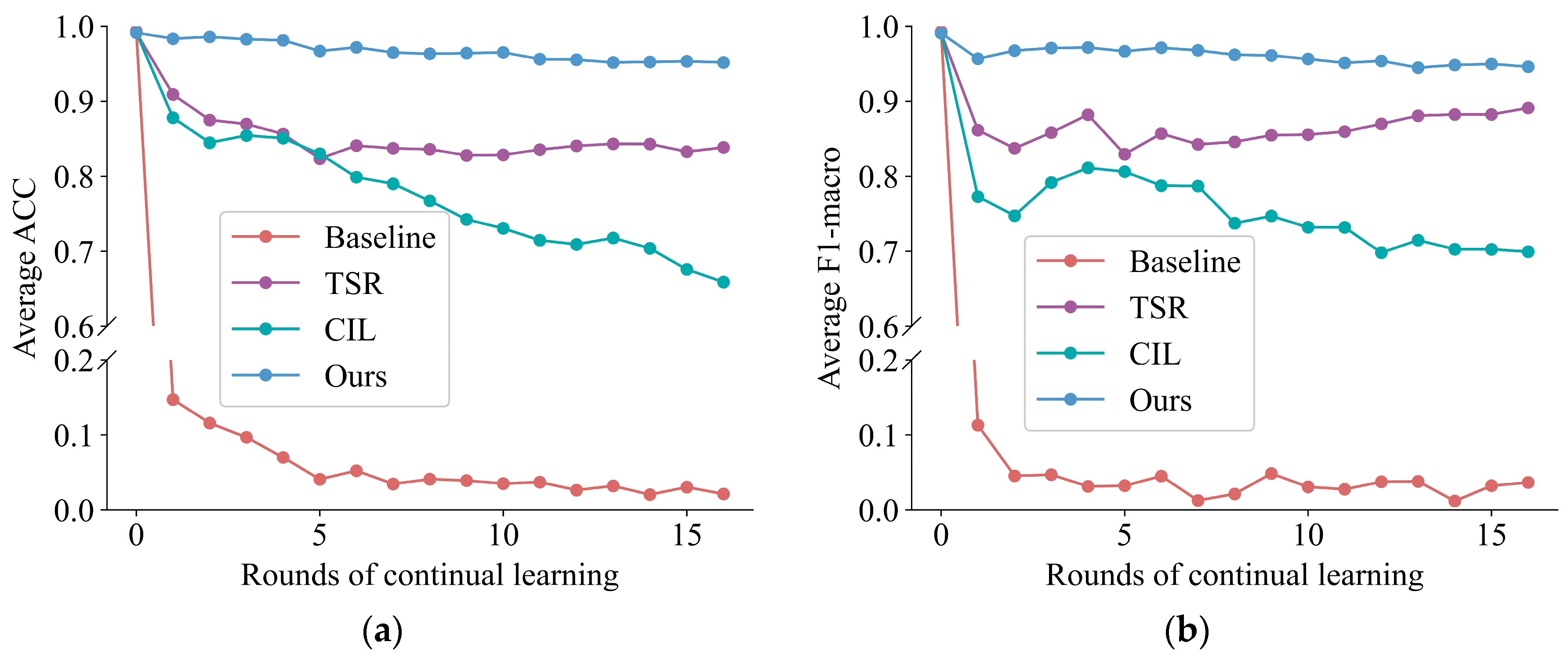
4.4. Experiment for Validating Analytic Continual Learning-Based Method in Load Identification

To validate the proposed continual learning-based NILM method in load identification, appliance types with over 200 samples across four public datasets are designated as common types, forming the dataset D₀ for pretraining the model. For the remaining appliances, a random set of every 3 types forms the streaming dataset D_k; that is, a total of 16 rounds of continual learning tasks are set up. For each appliance type, 80% of the samples are randomly selected for training, with the remaining used for testing. The following methods are used for comparation: (1) Freezing the feature extraction module and fine-tuning only the load identification branch as a baseline method without continual learning. (2) On the basis of freezing and then fine-tuning, DBSCAN-based typical waveform selection is added, and new data are jointly trained with the original data [11], denoted as TSR. The maximum number of stored samples per appliance type is set to 30. (3) The representative class-incremental learning method, incorporating knowledge distillation and output layer weight alignment in fine-tuning and simplifying waveform selection, based on average distance [14], is denoted as CIL. The maximum number of total stored samples for this method is set to 3000.

The performance of continual learning-based load identification is shown in Figure 3. Notably, the baseline method declines rapidly in performance. During the learning of D₁, it catastrophically forgets appliances from D₀ (the ACC drops from 0.99 to 0.07), and the loss of basic knowledge further hinders the learning of new appliances. This highlights the need to prevent catastrophic forgetting. After 16 rounds of continual learning, with the number of appliance types reaching 56, the ACC and F1-macro of the proposed method remain above 0.95 and 0.94, close to the performance of joint training with all the data. During the continual learning process, the proposed method degrades slowly and significantly outperforms the compared methods without requiring the storage of original data. In contrast, the two methods that store original data are less effective at mitigating catastrophic forgetting. As appliance types with fewer patterns arrive, TSR performs better and shows a slight increase in F1-macro by storing typical waveforms. In summary, the proposed method takes the practicality of continual learning-based load identification to a new height.

4.5. Experiment for Validating Analytic Continual Learning-Based Method in Novelty Detection

In the novelty detection experiment with continual learning settings, appliance types in the streaming data are divided in the same way as in Section 4.4. At the beginning of the experiment, appliances in the pretraining dataset D₀ are defined as the original appliances, and D₁ to D₁₆ are the new appliances. As continual learning progresses, D₁ to D₁₅ are sequentially transformed from new to original appliances. To ensure the presence of new appliances, the D₁₆ dataset is retained. Given the absence of continual learning-based novelty detection methods in NILM, the continual learning approaches from Section 4.4 are applied to the proposed novelty detection branch. Unlike the load identification branch, the novelty detection branch maintains a constant model capacity as new appliances arrive, updating the parameters to map their features into the hypersphere. As a result, novelty detection faces greater challenges in continual learning. The results are shown in Figure 4. The proposed method performs more stably during continual learning and outperforms the existing methods, with its accuracy consistently above 0.7. The new appliance types include resistive appliances with operating modes similar to the original appliances (e.g., ovens, shoe warmers, kettles) and appliances with distinct waveform patterns (e.g., water pumps, desoldering machines, shredders). These appliances activate the novelty detection branch to map inputs into the hypersphere, causing a drop in the F1-macro in later rounds due to misdetecting fewer new appliances than the original ones. In addition, the baseline method without continual learning suffers from catastrophic forgetting, reducing its performance to near-random guessing. TSR still outperforms CIL in novelty detection due to typical waveform selection, but its accuracy drops to 0.6 at the end.

4.6. Experiment for Validating the Proposed SCL-Based Pretraining Strategy

The above experiments show that the proposed method significantly outperforms the existing continual learning-based NILM methods without storing the original data. Based on the experiments in Section 4.4 and Section 4.5, this section strengthens the claim of the necessity of the proposed SCL strategy. The complete pretraining loss consists of cross-entropy (CE) loss and SCL loss, with both Gaussian (G) and random wandering (RW) noise used for data augmentation, as described in Section 3.3. It is compared with three alternatives: pure cross-entropy (CE), CE combined with SimCLR (an unsupervised contrastive loss) [26], and CE combined with SCL loss using only Gaussian noise (CE + SCL(G)). Comparing CE with CE + SCL(G + RN) directly verifies the necessity of SCL. Comparing CE + SimCLR with CE + SCL(G) demonstrates the effectiveness of supervised contrastive loss. Comparing CE + SCL(G) with CE + SCL(G + RN) serves as an ablation study for random wandering noise.

The results are shown in Figure 5. In load identification, the performance of CE + SCL(G + RN) is close to the optimal performance from joint training on D₀ to D₁₆, verifying the effectiveness of analytic continual learning. Pretraining with CE + SCL(G + RN) losses improves performance on the dataset D₀, as the feature space with greater distinctiveness between appliance types better satisfies the linear separability assumption for analytic continual learning. Moreover, the performance of the load identification model becomes more stable as the appliance types gradually increase. The final result shows a 1.8% improvement in the ACC and F1-macro compared to only using CE. In novelty detection, the CE + SCL(G + RN) offers greater advantages in this challenging continual learning task. In the initial rounds, a small number of appliances with the same operating mode (but mislabeled as unlearned types) are mapped to similar regions due to the enhanced feature representation from CE + SCL(G + RN)-based training. This label noise [4] leads to overly optimistic performance during training without the SCL strategy. In the continual learning process of novelty detection, the SCL-based pretraining strategy enhances feature space distinctiveness, making learned appliances less likely to be forgotten and improving overall stability. The final results show that CE + SCL(G + RN) improves the ACC by 32% and F1-macro by 18% compared to CE. If only the Gaussian noise is used for data augmentation in SCL, the performance is still better than CE, but after all the new appliance datasets are learned, identification and novelty detection accuracy are 1.1% and 14.8% lower, respectively. For unsupervised contrastive learning, SimCLR does not leverage the label information to enhance inter-type separation and intra-type clustering. In appliance identification, the model capacity increases with each new appliance, so the poor initial point from SimCLR pretraining has little impact on analytic continual learning. However, for novelty detection, where model capacity remains fixed, SimCLR-pretrained models tend to map almost all samples inside the hypersphere, classifying them as known appliances. Notably, as new datasets are added, the model’s accuracy increases in novelty detection simply because most samples are classified as known. When unknown samples are relabeled as known, the accuracy rises accordingly.

4.7. Validation of Hardware Deployment in Real-World Settings

To validate the proposed method in real-world environments, hardware deployment was implemented through pretraining, C code conversion, and chip programming, with the designed hardware being a smart socket comprising a high-power circuit board and a low-power circuit board interconnected via stacked pin headers to conserve space, as illustrated in Figure 6a,b. The core components of the high-power board include a plugin, power supply, relay, and sensor, while the low-power board handles data measurement, computation, and storage, utilizing an STM32F407 microcontroller (1 MB flash, 192 KB RAM) (STMicroelectronics, Geneva, Switzerland) as the edge computing core, a BL0956 chip (Belling, Shanghai, China) for high-frequency voltage/current sensing, an ESP32 Wi-Fi chip (Espressif Systems, Shanghai, China) for remote communication, and a W9825G6K chip (Winbond Electronics, Hsinchu, China) for expanded storage to enable NILM (non-intrusive load monitoring) feedback and manual appliance-type labeling. More than 21 types and a total of 151 appliances were prepared to mimic continual learning. For pretraining, device types with larger sample volumes were prioritized, with the streaming data partitioning detailed in

Table 3. The division of appliance types in streaming data.

Appliance Types in the Dataset	Role
D0: Hair dryer, induction cooker, fan, rice cooker, kettle, charger	Pretraining
D1: Disinfection cabinet, fridge, LED lamp	Continual learning
D2: Humidifier, iron, network switch	Continual learning
D3: Stove, TV, dehumidifier	Continual learning
D4: Electric bicycle, microwave, juice maker	Continual learning
D5: Electric blanket, incandescent light bulb, heater	Continual learning

. The overall partitioning principle is as follows: categories containing over 100 samples were allocated for pretraining, while the remaining classes, sorted in descending order by sample count, were grouped into triplets to form continual learning datasets. This approach stems from the observation that devices with higher sample volumes typically represent common real-world appliances, thereby facilitating easier access to trainable data. Conversely, devices with sparse samples are less likely to be captured during initial sampling; they are gradually integrated and discovered through prolonged monitoring, making them more suitable as incremental targets for continual learning. To ensure the presence of new appliances in the novelty detection experiment, the D₅ dataset was retained. As in previous experiments, about 20% of the appliances in each type are reserved for testing. For new appliances, the waveforms to be learned are saved locally, and the type labels are sent manually to the hardware via the host computer. After the hardware completes continual learning, the appliances are manually plugged in or unplugged for testing. The experimental environment is shown in Figure 6c.

The results are shown in Figure 7. In load identification, the similarity in operating patterns between power electronic appliances (e.g., chargers, computers, TV) and resistive appliances (e.g., disinfection cabinet, rice cooker, heater) increases identification difficulty, reducing performance by about 10% compared to the public datasets. Despite this, load identification performance fluctuates by less than 5% during continual learning as the number of appliance types expands to 21, making it feasible for practical application. In novelty detection, provided that the misclassification of new appliances as original types is correctable via user feedback, attention is restricted to cases where original appliances are misclassified as new, representing approximately 20% of the instances requiring relabeling. This ratio is acceptable for practical applications. Interestingly, as more new appliances with similar operating modes, initially mapped within the hypersphere, are correctly detected after their labels are transformed into learned appliances, the ACC increases in later rounds of continual learning. Whereas F1-macro declines slightly, as the model is more likely to misdetect new appliances as original ones in later rounds, which is consistent with the public datasets. For hardware operation efficiency, load identification and novelty detection for a single appliance take only 1.75 s and 3.24 s, respectively. The analytic continual learning for 16 appliances takes 1053.44 s for load identification and 316.03 s for novelty detection due to increased matrix computations. It should be clarified that the continual learning program does not need to run in real time. Even without the hardware acceleration techniques, such as sparse computation, its running time remains within acceptable limits.

5. Conclusions

To address the continual emergence of new appliances, a NILM method based on analytic continual learning is proposed, eliminating the complexity and data leakage risk of the existing methods that require storing original appliance data. The designed NILM model consists of a 1D depthwise separable convolution-based feature extraction module and dual output branches for load identification and novelty detection. It is further optimized for appliance-type distinctiveness in the feature space by the proposed SCL-based pretraining strategy. When new appliance data arrive, the novelty detection branch first determines whether learning is required. The analytic continual learning method then updates the load identification and novelty detection branches using only new data, realizing a closed-loop iteration of novelty detection-continual learning in streaming load data. The experimental results show that optimizing the learning process with the proposed method enables the NILM model to match the best performance of existing load identification and novelty detection methods while reducing the computational effort by 70.44%. Moreover, the proposed method exhibits a more stable continual learning ability when appliance types are added when compared to the methods that need to store original data. As appliance types are added from 8 to 56, the accuracy of load identification and novelty detection is 13.52% and 15.33% higher than the best existing method. In addition, the proposed method is deployed on an STM32F407-based smart socket, meeting real-world NILM performance requirements within an acceptable execution time. Overall, a novel and practical solution is presented for continual learning in NILM.

In the future, we will focus on the following challenges: (1) Improving novelty detection performance by exploring strategies such as dynamically expanding the model’s capacity as the number of appliance types increases. (2) Combining sample selection methods from active learning [39] to reduce the amount of labeling required for new appliances. (3) Promoting the application of smart sockets by deploying the proposed method to validate it across a wider variety of appliances.

References

1. Liu, Y.; Wang, Y.; Ma, J. Non-Intrusive Load Monitoring in Smart Grids: A Comprehensive Review. arXiv 2024, arXiv:2403.06474. [Google Scholar]
2. Mari, S.; Bucci, G.; Ciancetta, F.; Fiorucci, E.; Fioravanti, A. A review of non-intrusive load monitoring applications in industrial and residential contexts. Energies 2022, 15, 9011. [Google Scholar] [CrossRef]
3. Ji, T.; Chen, J.; Zhang, L.; Lai, H.; Wang, J.; Wu, Q. Low frequency residential load monitoring via feature fusion and deep learning. Electr. Power Syst. Res. 2025, 238, 111092. [Google Scholar] [CrossRef]
4. Luo, Q.; Yu, T.; Lan, C.; Huang, Y.; Wang, Z.; Pan, Z. A Generalizable Method for Practical Non-Intrusive Load Monitoring via Metric-Based Meta-Learning. IEEE Trans. Smart Grid 2024, 15, 1103–1115. [Google Scholar] [CrossRef]
5. Liu, Y.; Wang, X.; You, W. Non-Intrusive Load Monitoring by Voltage–Current Trajectory Enabled Transfer Learning. IEEE Trans. Smart Grid 2019, 10, 5609–5619. [Google Scholar] [CrossRef]
6. McCloskey, M.; Cohen, N.J. Catastrophic interference in connectionist networks: The sequential learning problem. In Psychology of Learning and Motivation; Elsevier: Amsterdam, The Netherlands, 1989; Volume 24, pp. 109–165. [Google Scholar]
7. D’Incecco, M.; Squartini, S.; Zhong, M. Transfer Learning for Non-Intrusive Load Monitoring. IEEE Trans. Smart Grid 2020, 11, 1419–1429. [Google Scholar] [CrossRef]
8. Wang, L.; Mao, S.; Wilamowski, B.M.; Nelms, R.M. Pre-Trained Models for Non-Intrusive Appliance Load Monitoring. IEEE Trans. Green Commun. Netw. 2022, 6, 56–68. [Google Scholar] [CrossRef]
9. Wang, L.; Zhang, X.; Su, H.; Zhu, J. A comprehensive survey of continual learning: Theory, method and application. IEEE Trans. Pattern Anal. Mach. Intell. 2024, 46, 5362–5383. [Google Scholar] [CrossRef]
10. Sykiotis, S.; Kaselimi, M.; Doulamis, A.; Doulamis, N. Continilm: A Continual Learning Scheme for Non-Intrusive Load Monitoring. In Proceedings of the ICASSP 2023—2023 IEEE International Conference on Acoustics, Speech and Signal Processing (ICASSP), Rhodes Island, Greece, 4–10 June 2023; pp. 1–5. [Google Scholar]
11. Zhang, J.; Tan, Z.; Gao, J.; Liu, B.; Zeng, P. A Generalizability-Enhancing Method for Load Identification Based on Typical Sample Replay. In Proceedings of the 2023 3rd International Conference on Computer Science, Electronic Information Engineering and Intelligent Control Technology (CEI), Wuhan, China, 13–15 December 2023; pp. 683–687. [Google Scholar]
12. Yin, L.; Ma, C. Interpretable Incremental Voltage–Current Representation Attention Convolution Neural Network for Nonintrusive Load Monitoring. IEEE Trans. Ind. Inf. 2023, 19, 11776–11787. [Google Scholar] [CrossRef]
13. Zhou, R.; Fang, X. Non-intrusive Load Monitoring Based Data-Free Incremental Electrical Appliance Identification. In Proceedings of the International Conference on Energy and Environmental Science, Chongqing, China, 5–7 January 2024; pp. 869–879. [Google Scholar]
14. Qiu, L.; Yu, T.; Lan, C. A semi-supervised load identification method with class incremental learning. Eng. Appl. Artif. Intell. 2024, 131, 107768. [Google Scholar] [CrossRef]
15. Tanoni, G.; Principi, E.; Mandolini, L.; Squartini, S. Appliance-Incremental Learning for Non-Intrusive Load Monitoring. In Proceedings of the 2023 IEEE International Conference on Communications, Control, and Computing Technologies for Smart Grids (SmartGridComm), Glasgow, UK, 31 October–3 November 2023; pp. 1–6. [Google Scholar]
16. Guo, X.; Wang, C.; Wu, T.; Li, R.; Zhu, H.; Zhang, H. Detecting the novel appliance in non-intrusive load monitoring. Appl. Energy 2023, 343, 121193. [Google Scholar] [CrossRef]
17. Kang, J.-S.; Yu, M.; Lu, L.; Wang, B.; Bao, Z. Adaptive Non-Intrusive Load Monitoring Based on Feature Fusion. IEEE Sens. J. 2022, 22, 6985–6994. [Google Scholar] [CrossRef]
18. Zhao, Q.; Liu, W.; Li, K.; Wei, Y.; Han, Y. Unknown appliances detection for non-intrusive load monitoring based on vision transformer with an additional detection head. Heliyon 2024, 10, e30666. [Google Scholar] [CrossRef] [PubMed]
19. Gao, A.; Zheng, J.; Mei, F.; Sha, H.; Xie, Y.; Li, K.; Liu, Y. Non-intrusive multi-label load monitoring via transfer and contrastive learning architecture. Int. J. Electr. Power Energy Syst. 2023, 154, 109443. [Google Scholar] [CrossRef]
20. Lu, L.; Kang, J.-S.; Meng, F.; Yu, M. Non-intrusive load identification based on retrainable siamese network. Sensors 2024, 24, 2562. [Google Scholar] [CrossRef]
21. Chollet, F. Xception: Deep learning with depthwise separable convolutions. In Proceedings of the IEEE Conference on Computer Vision and Pattern Recognition, Honolulu, HI, USA, 21–26 July 2017; pp. 1251–1258. [Google Scholar]
22. Ioffe, S.; Szegedy, C. Batch normalization: Accelerating deep network training by reducing internal covariate shift. In Proceedings of the International Conference on Machine Learning, Lille, France, 6–11 July 2015; pp. 448–456. [Google Scholar]
23. Faustine, A.; Pereira, L.; Klemenjak, C. Adaptive Weighted Recurrence Graphs for Appliance Recognition in Non-Intrusive Load Monitoring. IEEE Trans. Smart Grid 2021, 12, 398–406. [Google Scholar] [CrossRef]
24. Ruff, L.; Vandermeulen, R.; Goernitz, N.; Deecke, L.; Siddiqui, S.A.; Binder, A.; Müller, E.; Kloft, M. Deep one-class classification. In Proceedings of the International Conference on Machine Learning, Stockholm, Sweden, 10–15 July 2018; pp. 4393–4402. [Google Scholar]
25. Khosla, P.; Teterwak, P.; Wang, C.; Sarna, A.; Tian, Y.; Isola, P.; Maschinot, A.; Liu, C.; Krishnan, D. Supervised contrastive learning. Adv. Neural Inf. Process. Syst. 2020, 33, 18661–18673. [Google Scholar]
26. Zhao, R.; Lu, J.; Liu, B.; Yu, Z.; Ren, Y.; Zheng, W. Non-Intrusive Load Identification Method Based on Self-Supervised Regularization. IEEE Access 2023, 11, 144696–144704. [Google Scholar] [CrossRef]
27. Box, G.E.; Jenkins, G.M.; Reinsel, G.C.; Ljung, G.M. Time Series Analysis: Forecasting and Control; John Wiley & Sons: Hoboken, NJ, USA, 2015. [Google Scholar]
28. Zhuang, H.; Weng, Z.; Wei, H.; Xie, R.; Toh, K.-A.; Lin, Z. ACIL: Analytic class-incremental learning with absolute memorization and privacy protection. Adv. Neural Inf. Process. Syst. 2022, 35, 11602–11614. [Google Scholar]
29. Zhuang, H.; Fang, D.; Tong, K.; Liu, Y.; Zeng, Z.; Zhou, X.; Chen, C. Online Analytic Exemplar-Free Continual Learning with Large Models for Imbalanced Autonomous Driving Task. IEEE Trans. Veh. Technol. 2024, 74, 1949–1958. [Google Scholar] [CrossRef]
30. Zhuang, H.; Yan, Y.; He, R.; Zeng, Z. Class incremental learning with analytic learning for hyperspectral image classification. J. Franklin Inst. 2024, 361, 107285. [Google Scholar] [CrossRef]
31. Woodbury, M.A. Inverting Modified Matrices; Department of Statistics, Princeton University: Princeton, NJ, USA, 1950. [Google Scholar]
32. Medico, R.; De Baets, L.; Gao, J.; Giri, S.; Kara, E.; Dhaene, T.; Develder, C.; Berges, M.; Deschrijver, D. A voltage and current measurement dataset for plug load appliance identification in households. Sci. Data 2020, 7, 49. [Google Scholar] [CrossRef] [PubMed]
33. Houidi, S.; Fourer, D.; Auger, F.; Sethom, H.B.A.; Miegeville, L. Home electrical appliances recordings for NILM. IEEE DataPort 2020. [Google Scholar] [CrossRef]
34. Kahl, M.; Haq, A.U.; Kriechbaumer, T.; Jacobsen, H.-A. Whited-a worldwide household and industry transient energy data set. In Proceedings of the 3rd International Workshop on Non-Intrusive Load Monitoring, Vancouver, BC, Canada, 14–15 May 2016; pp. 1–4. [Google Scholar]
35. Picon, T.; Meziane, M.N.; Ravier, P.; Lamarque, G.; Novello, C.; Bunetel, J.-C.L.; Raingeaud, Y. COOLL: Controlled on/off loads library, a public dataset of high-sampled electrical signals for appliance identification. arXiv 2016, arXiv:1611.05803. [Google Scholar]
36. Virtanen, P.; Gommers, R.; Oliphant, T.E.; Haberland, M.; Reddy, T.; Cournapeau, D.; Burovski, E.; Peterson, P.; Weckesser, W.; Bright, J. SciPy 1.0: Fundamental algorithms for scientific computing in Python. Nat. Methods 2020, 17, 261–272. [Google Scholar] [CrossRef]
37. Zhang, Y.; Wu, H.; Ma, Q.; Yang, Q.; Wang, Y. A Learnable Image-Based Load Signature Construction Approach in NILM for Appliances Identification. IEEE Trans. Smart Grid 2023, 14, 3841–3849. [Google Scholar] [CrossRef]
38. Liu, Y.; Xu, Q.; Yang, Y.; Zhang, W. Detection of Electric Bicycle Indoor Charging for Electrical Safety: A NILM Approach. IEEE Trans. Smart Grid 2023, 14, 3862–3875. [Google Scholar] [CrossRef]
39. Fu, Y.; Zhu, X.; Li, B. A survey on instance selection for active learning. Knowl. Inf. Syst. 2013, 35, 249–283. [Google Scholar] [CrossRef]
Figure 1. Overview of the proposed NILM framework for adapting to new appliances. SCL stands for supervised contrastive learning, ACL for analytic continual learning, DS-Conv for depthwise separable convolution, 1D-Conv for one-dimensional convolution, BN for batch normalization, and FC for a fully connected layer.
Applsci 15 06571 g001
Figure 2. The raw appliance waveforms and the augmented waveforms with a signal-to-noise ratio of 5 dB: (a) air conditioner (raw waveform); (b) air conditioner (with random wandering noise); (c) air conditioner (with Gaussian noise); (d) Halogen Fluter (raw waveform); (e) Halogen Fluter (with random wandering noise); (f) Halogen Fluter (with Gaussian noise).
Applsci 15 06571 g002
Figure 3. The average performance of continual learning-based methods in load identification: (a) ACC and (b) F1-macro.
Applsci 15 06571 g003
Figure 4. The average performance of continual learning-based methods in novelty detection: (a) ACC and (b) F1-macro.
Applsci 15 06571 g004
Figure 5. The average performance with and without SCL-based pretraining strategy: (a) load identification (ACC); (b) load identification (F1-macro); (c) novelty detection (ACC); (d) novelty detection (F1-macro).
Applsci 15 06571 g005aApplsci 15 06571 g005b
Figure 6. The platform for the hardware deployment experiment: (a) strong electrical board; (b) weak electrical board; (c) experimental environment using the smart socket.
Applsci 15 06571 g006
Figure 7. The average performance in hardware deployment: (a) load identification (ACC); (b) load identification (F1-macro); (c) novelty detection (ACC); (d) novelty detection (F1-macro).
Applsci 15 06571 g007