Multi-Scenario Robust Distributed Permutation Flow Shop Scheduling Based on DDQN

Abstract

In order to address the Distributed Displacement Flow Shop Scheduling Problem (DPFSP) with uncertain processing times in real production environments, Plant Simulation is employed to construct a simulation model for the MSRDPFSP. The model conducts quantitative analyses of workshop layout, assembly line design, worker status, operating status of robotic arms and AGV vehicles, and production system failure rates. A hybrid NEH-DDQN algorithm is integrated into the simulation model via a COM interface and DLL, where the NEH algorithm ensures the model maintains optimal performance during the early training phase. Four scheduling strategies are designed for workpiece allocation across different workshops. A deep neural network replaces the traditional Q-table for greedy selection among these four scheduling strategies, using each workshop’s completion time as a simplified state variable. This approach reduces algorithm training complexity by abstracting away intricate workpiece allocation details. Experimental comparisons show that for the data of 500 workpieces, the NEH algorithm in 3 s demonstrates equivalent quality to that produced by the GA algorithm in 300 s. After 2000 iterations, the DDQN algorithm achieves a 15% reduction in makespan with only a 2.5% increase in computational time compared to random search, this joint simulation system offers an efficient and stable solution for the modeling and optimization of the MSRDPFSP issue.

1. Introduction

Since the early 21st century, the manufacturing industry has entered a new era of intelligentization, informatization, and automation [1,2]. With continuous breakthroughs in cutting-edge technologies such as artificial intelligence, the Internet of Things, robotics, and big data analytics, intelligent manufacturing has emerged as a key strategic approach for countries aiming to enhance their industrial competitiveness. As globalized production expands and manufacturing scales increase, enterprises face increasingly complex and diversified market demands. To maintain a competitive edge in the global market, large manufacturing enterprises are actively exploring ways to reduce production costs, improve efficiency, and enhance production flexibility. In this context, manufacturing paradigms are undergoing a fundamental shift from traditional centralized workshop-based production models to distributed production systems.

The DPFSP refers to the simultaneous processing of multiple jobs across multiple factories or production lines, where jobs may be reassigned or permuted between different factories. The objective is typically to minimize the total completion time (makespan). The problem was first formally introduced by Naderi and Ruiz [3], who proposed six mixed-integer linear programming formulations based on different modeling perspectives. Following this foundational study, contributions to the DPFSP literature have steadily increased.

Ruiz et al. [4] proposed a series of dispatching rules based on heuristics or experiences to optimize flow shop scheduling problems. These rules offer simplicity and practicality, enabling high-quality near-optimal solutions with relatively low computational costs. Xiong et al. [5] extended traditional routing-based dispatching rules using a simulation-driven approach and conducted a systematic evaluation of rule performance in dynamic environments, emphasizing the need for responsive and robust scheduling strategies in settings with complex constraints.

Deng et al. [6] introduced a novel competitive memetic algorithm. This algorithm effectively improves global optimization performance by dividing the search space and employing multiple subpopulations for localized search. Lu et al. [7] proposed an improved hybrid tabu search algorithm, which enhances traditional tabu search by incorporating problem-specific features and optimization objectives to improve performance and computational efficiency. Ruiz et al. [8] also introduced an iterative greedy algorithm. This method is particularly well-suited for solving scheduling challenges involving complex constraints and multiple objectives, such as those encountered in production scheduling and logistics optimization.

Gogos [9] proposed an innovative approach in solving DPFSP to optimize the scheduling scheme utilizing constraint planning techniques. Li et al. [10] developed a self-adaptive population-based iterated greedy algorithm to address the DPFSP.

With the advancement of intelligent technologies, emerging methods such as DQN and hybrid algorithms have provided powerful tools to address large-scale, dynamic, and complex DPFSP scenarios. By integrating uncertainty into the state and reward functions, Zhao et al. [11] explored the application of Q-learning to DPFSP with uncertain processing times, enabling agents to dynamically adjust decisions based on learned experiences.

Wang et al. [12] designed a K-means-based workload allocation rule to balance load among factories and applied Deep Q-Network to capture nonlinear relationships between states and actions. This enables the agent to generalize and solve problems of different scales after training.

Due to the inherent complexity of DPFSP, no single algorithm has yet demonstrated superior performance across all scenarios [13]. Most existing studies focus on specific cases by simplifying problem models or assuming fewer real-world constraints to improve computational performance. However, in real manufacturing environments, numerous uncontrollable and uncertain factors—such as machine aging and failure, variations in operator skill levels, unstable material supply, and external environmental changes—can significantly affect system stability and scheduling effectiveness. These uncertainties are often challenging to predict during the planning phase, resulting in deviations between deterministic scheduling models and actual production. Consequently, this affects the feasibility and robustness of solutions.

Therefore, research on the MSRDPFSP is of great significance. It not only improves scheduling stability in complex and dynamic manufacturing environments but also holds substantial economic value and practical application potential [14].

Zhang and Cai [15] proposed a collaborative optimization framework integrating dual population genetic algorithm and Q-learning for multi-objective DPFSP. Zhou et al. [16] proposed a bio-inspired reinforcement learning method to tackle the robustness challenges in replacement flow shop scheduling, offering a bio-inspired solution for adaptive scheduling in smart manufacturing environments. Waubert et al. [17] conducted a comprehensive survey of reinforcement learning-based production scheduling systems, highlighting the challenges in applying such methods to industrial environments, such as high training costs and limited model stability. Souza et al. [18] addressed machine unavailability due to preventive and corrective maintenance in job shop scheduling by proposing a robust scheduling method that incorporates both deterministic and stochastic unavailability constraints. This method enhances system stability and execution reliability amid uncertainty. Luo et al. [19] proposed a hybrid optimization approach combining Estimation of Distribution Algorithm and Proximal Policy Optimization. Gu et al. [20] devised a DQN approach within a multi-agent system architecture to tackle dynamic disturbances, including uncertain processing times, order changes, and machine failures. This framework provides a novel strategy for real-time scheduling in intelligent manufacturing environments, enabling adaptive response to runtime uncertainties.

However, solving the MSRDPFSP using traditional algorithms is extremely time-consuming, particularly in simulation-based environments. Against this backdrop, digital transformation has provided strong support for technological innovation and industrial upgrading in intelligent manufacturing. By using Plant Simulation to establish digital twin models of existing workflows, Malega et al. [21] improved resource allocation efficiency. Fedoko et al. [22] innovatively applied Plant Simulation to traffic node modeling and optimization, achieving dynamic simulation and 3D visualization of vehicle operation, congestion formation, and delay situations. Sobrino et al. [23] simulated the logic verification of manufacturing systems using Plant Simulation, enabling rapid verification and optimization of control logic in manufacturing systems, thereby significantly reducing costs and risks during the actual debugging phase. Zhao et al. [24] proposed an assembly flow shop scheduling optimization method integrating virtual simulation and a migratory bird optimization algorithm. They established a virtual simulation environment incorporating digital twin technology and enabled real-time performance evaluation of scheduling schemes. Recent studies have demonstrated Plant Simulation as a discrete event simulation tool—a tool boasting significant advantages in modeling complex systems in the manufacturing industry [25,26,27]. Digital modeling enables real-time access to production environment data while supporting efficient simulation, which significantly improves the accuracy and feasibility of solving complex scheduling problems under MSRDPFSP scenarios. Despite these advantages, most existing digital simulation platforms still rely on exhaustive search strategies for scheduling. As the problem scale expands, this leads to a dramatic increase in computational complexity, making the optimization of scheduling sequences increasingly time-consuming and less efficient.

This paper presents a hybrid simulation system that models the MSRDPFSP using Plant Simulation to address scheduling sequence simulation time. The system more accurately replicates complex real-world production environments compared to traditional methods. The DDQN algorithm retrieves model simulation results via the COM interface or DLL, enabling iterative learning from initial populations generated by the NEH algorithm to rapidly balance maximum completion times across workshops. The main contributions of this work are summarized as follows:

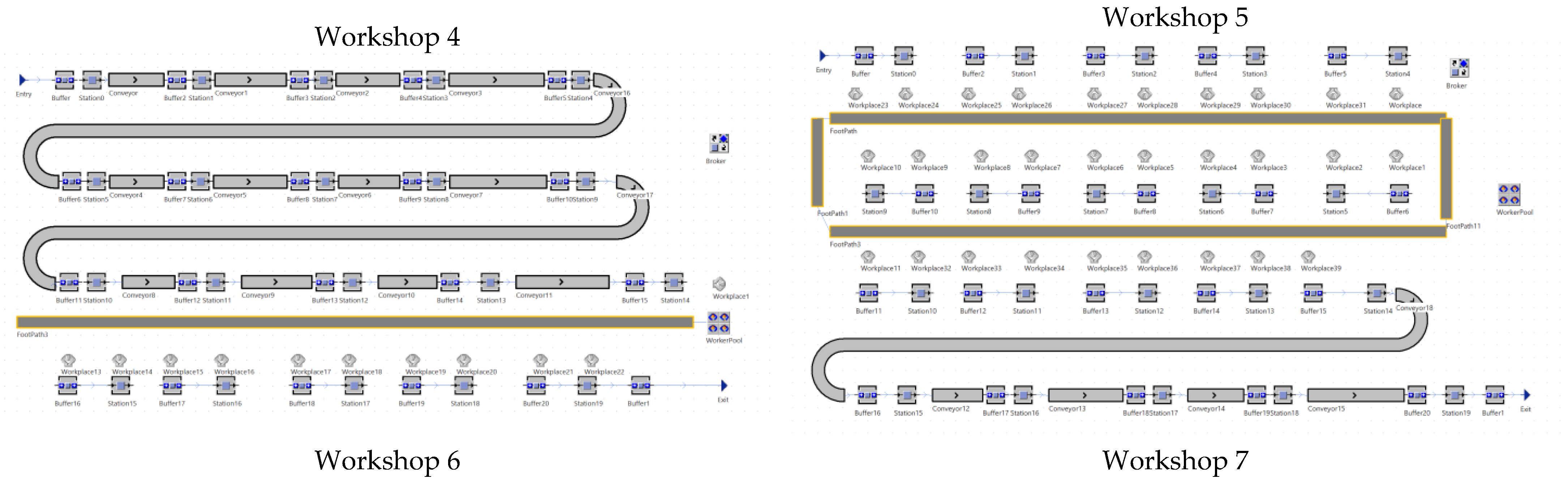
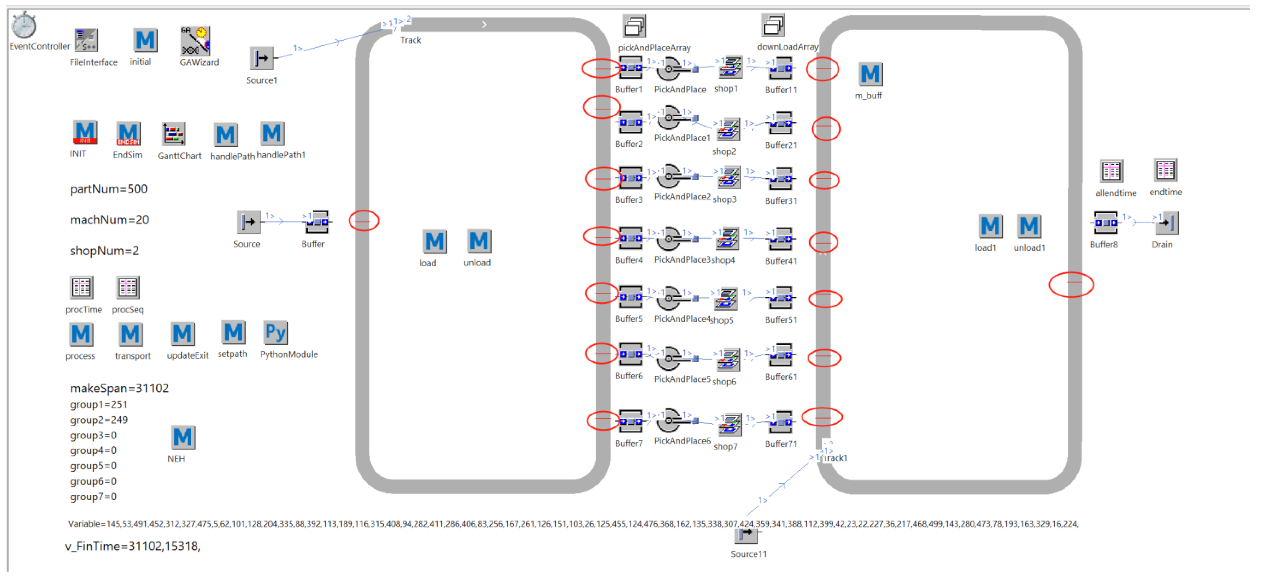
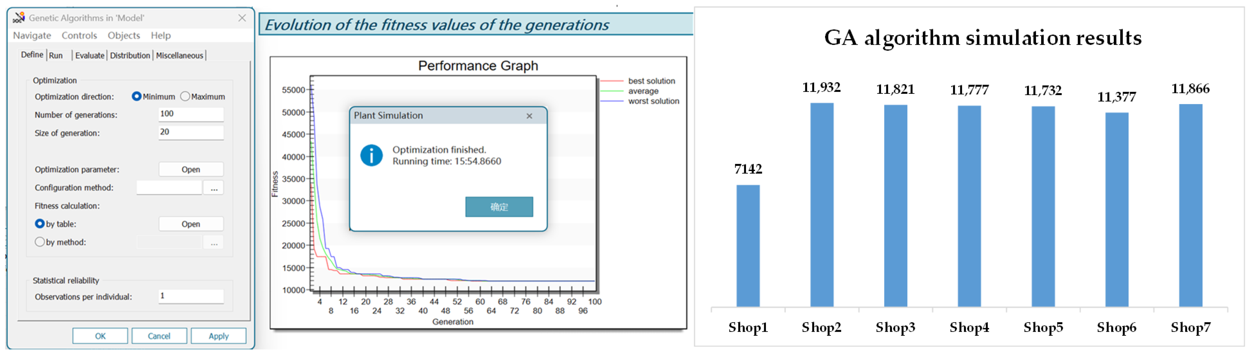
• Siemens Plant Simulation is employed to digitally model the distributed workshop through the definition of operational processes, dynamic events, scheduling rules, and optimization goals. To simulate the complexity of real-world production environments, seven distinct factory types are designed to quantitatively analyze the workshop layout, assembly line design, the state of the workers, robotic arms, AGV vehicles, and other production system parameters. Fault rates are incorporated into the production system to maximize the reproduction of the real production environment. Moreover, GA components are employed to optimize the production process, greatly improving production efficiency.
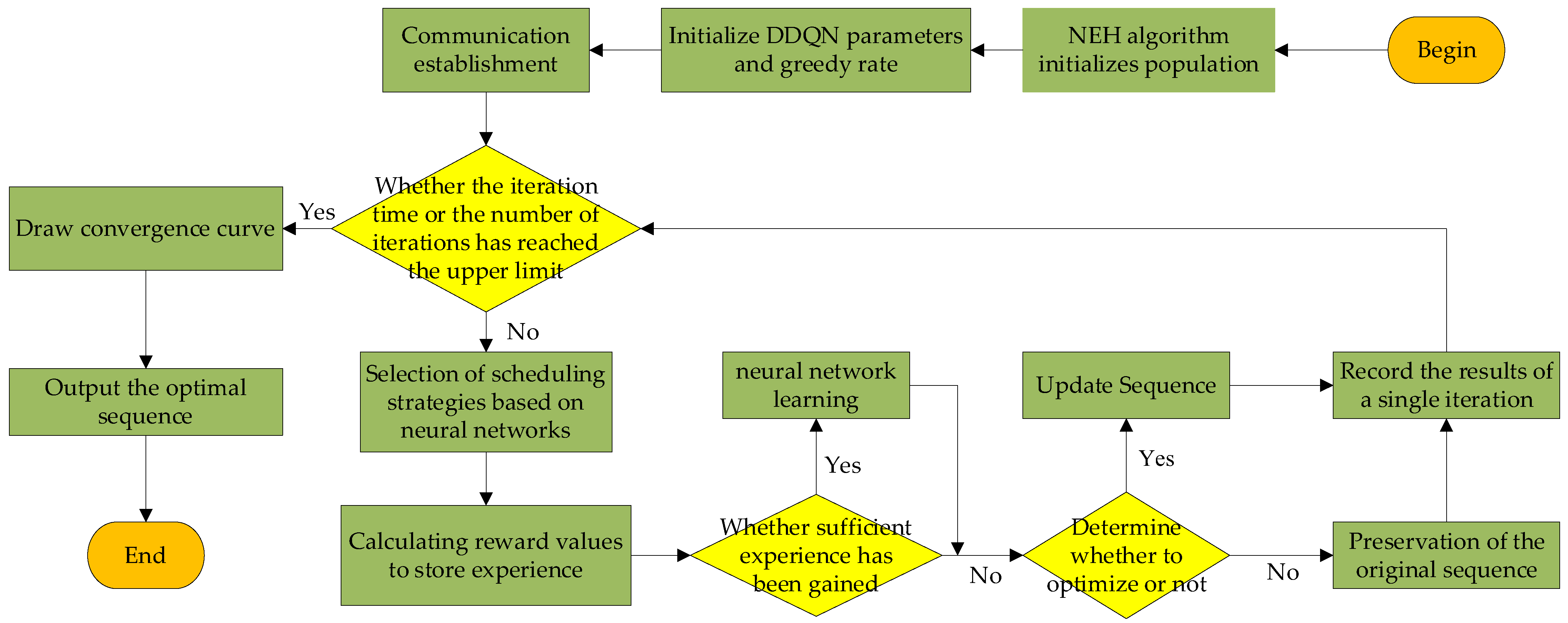
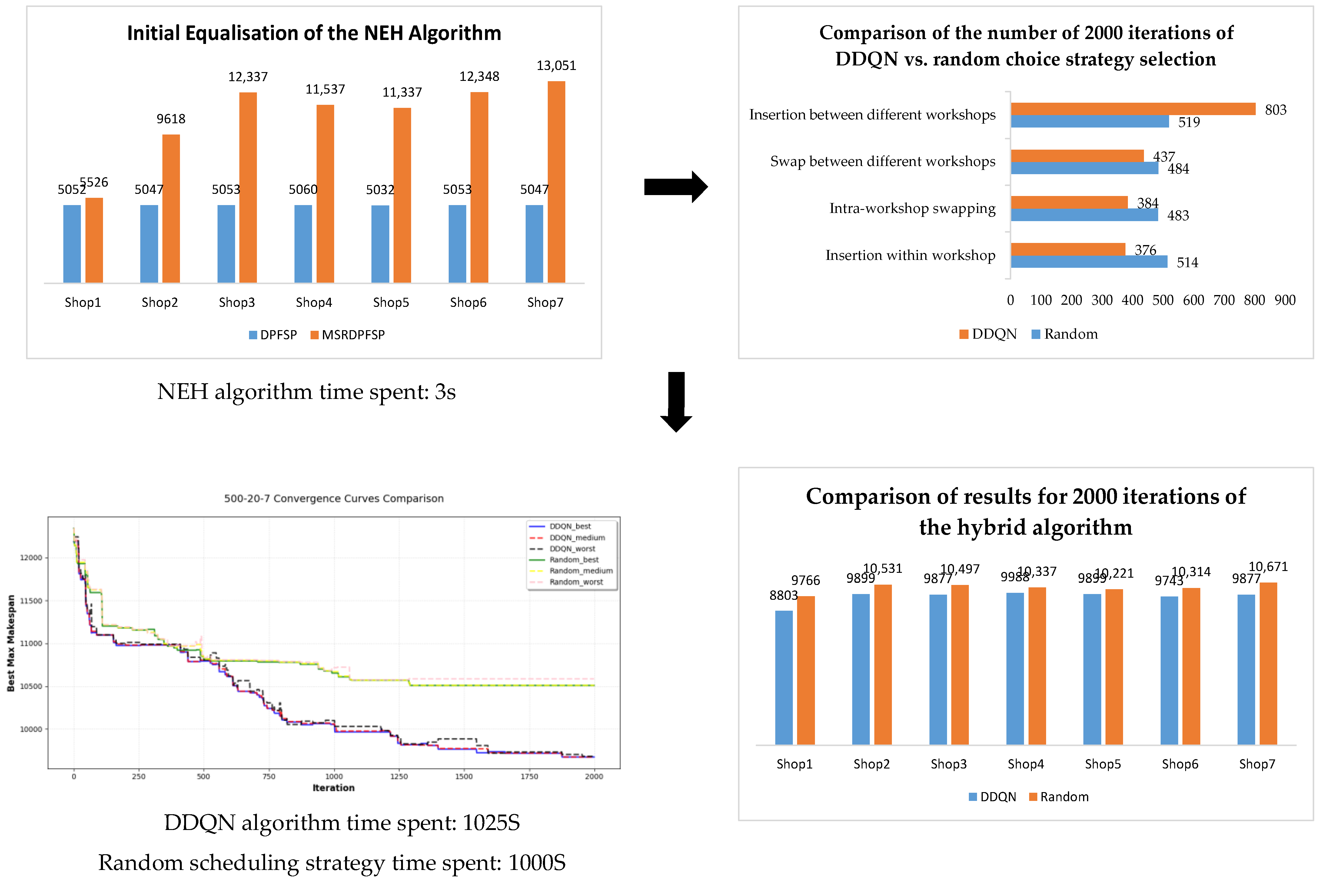
• An approximate optimal solution is generated for the DPFSP using the NEH algorithm and used as the initial solution for MSRDPFSP. Four search strategies are designed, with DQN introduced to minimize the processing time as the target for evaluating Q values. Greedy selection is performed among the four search strategies. The DDQN approach separates the Target Network and the Evaluation Network to mitigate the overestimation of Q-values. Additionally, the allocation information of the workpieces is replaced with the makespan of each workshop as the state information, reducing the training difficulty of the neural network.
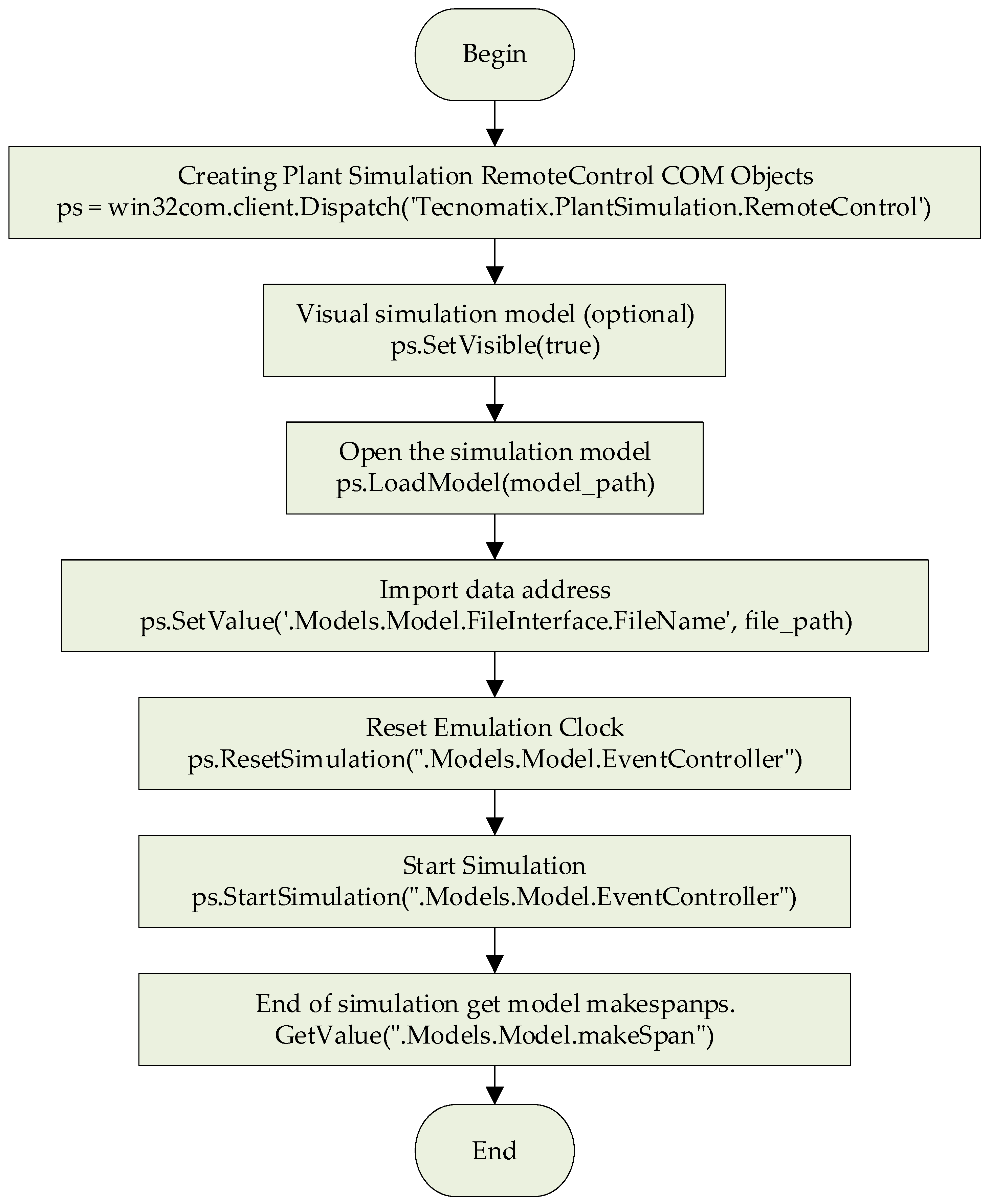
• Using the COM interface of Plant Simulation, the models in Plant Simulation are controlled through Pytharm to retrieve simulation results, while calculation and analysis functions in Pytharm are invoked through Plant Simulation. The hybrid DDQN-NEH algorithm is directly integrated into the MSRDPFSP simulation model via DLL, thus completing the entire link from modeling, optimization, to simulation.

The remaining chapters of this paper are structured as follows: Section 2 introduces some basic concepts of the research content; Section 3 constructs a digital simulation model of DPFSP using Plant Simulation reference Taillard dataset and thus builds a MSRDPFSP simulation model by increasing the scenario complexity as well as the robustness; Section 4 elaborates on the design of the hybrid DDQN-NEH algorithm proposed in this paper and its interaction with the simulation model established in Section 3; Section 5 evaluates the performance of this joint simulation system; Section 6 delineates the experimental protocol and engages in a comprehensive discourse on the findings; and Section 7 furnishes the conclusions, highlights the study’s limitations, and illuminates avenues for future exploration.

2. Related Theory

2.1. The Distributed Replacement Flow Shop Scheduling Problem

The DPFSP refers to the assignment of multiple workpieces to be processed on an assembly line in multiple shops, where each workpiece is required to go through multiple processes in sequence. Moreover, the workpieces can be displaced in different shops, with the goal of minimizing the total completion time of all the workpieces [28]. Two subproblems should be considered simultaneously in DPFSP: the allocation of workpieces between workshops and the sequencing of workpieces within workshops. The problem can be described as follows: there are F identical workshops and M identical machines in each workshop. N workpieces are assigned to be processed in each workshop. A conceptual diagram of the distributed workshop is shown in Figure 1 below.

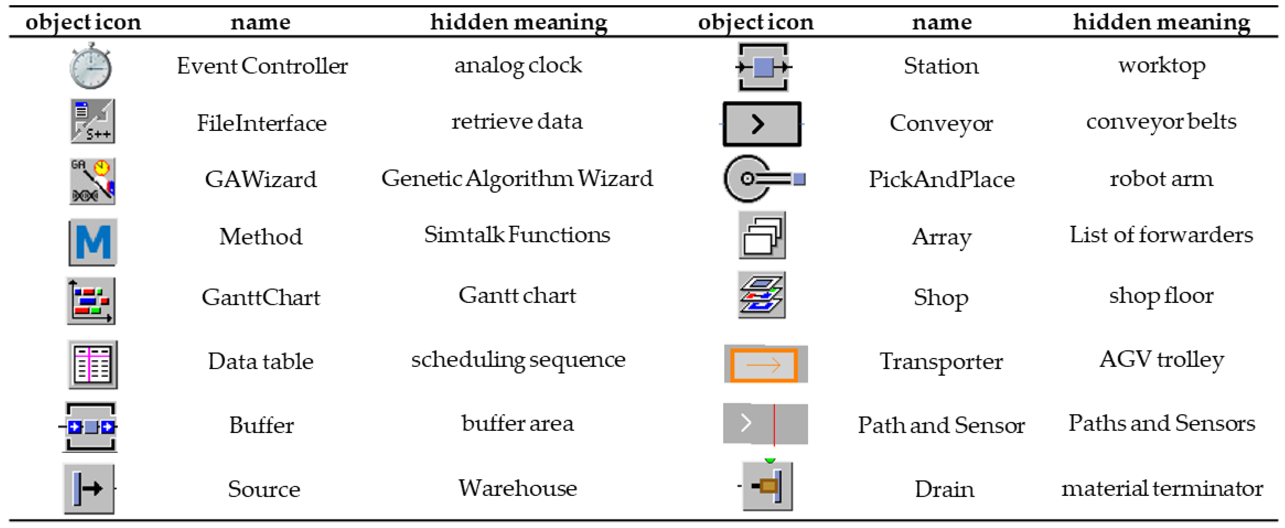
2.2. Computer Simulation Software Plant Simulation

Computer simulation software, as a multifunctional tool, not only covers the construction of simulation models and the storage of simulation data but also has the ability to analyze the simulation results in depth [29]. Plant Simulation is a software tool for discrete-event simulation introduced by Siemens, extensively used in the modeling, optimization, and analysis of production systems [30]. Through simulation, complex production processes can be modeled and optimized in a digital environment to improve productivity, resource utilization, and responsiveness [31]. The model elements in the Plant Simulation software used in this paper, along with their names and meanings, are shown in Figure 2 below.

2.3. NEH and DDQN Algorithms

The NEH algorithm is widely used to generate high-quality initial scheduling sequences [32]. Its core idea is to sort the workpieces in descending order according to their total machining time in each process. Workpieces are then sequentially inserted into all possible positions in the currently constructed scheduling sequence. For each insertion position, the makespan is calculated, and the position yielding the minimum makespan is selected. This process iteratively extends the existing scheduling sequence until all the artifacts are inserted. Figure 3 below illustrates a simplified flowchart of seven tasks assigned to three workshops.

The core of reinforcement learning is the process by which an agent learns to obtain the best behavior based on environmental rewards, i.e., there exists a mapping relationship between the state and the action [33]. This mechanism learns to maximize cumulative rewards by iteratively refining the policy through exploration and exploitation. The agent continuously experiments in the environment and optimizes the state–action correspondence through the inverse of the environment.

DDQN is a deep reinforcement learning algorithm optimized and improved on the basis of DQN. Its main goal is to alleviate the overestimation of Q value that tends to occur in the training process of DQN. In DQN, both the selection of actions and the evaluation of action values are performed by the same neural network, and this mechanism often leads to the Q-value deviating from the actual return, thus affecting the optimality and convergence of the strategy. To solve this problem, DDQN introduces two independent neural networks: the Evaluation Network used to select the optimal action in the current state, and the Target Network responsible for evaluating the value of the action. This improves the stability of the policy learning through the separation mechanism of action selection and action evaluation, effectively reduces the Q-value estimation bias, and demonstrates superior stability in addressing workshop scheduling problems [34].

3. Simulation Model

Intelligent manufacturing is not only a key component of Industry 4.0, but also a core driving force to promote the transformation and upgrading of the manufacturing industry [35]. Through the deep integration of informatization, digitalization, automation, and intelligence, intelligent manufacturing can significantly improve production efficiency, reduce production costs, improve product quality, and enhance production flexibility. In intelligent manufacturing, the production workshop is endowed with more intelligent functions, such as completing the assembly, testing, and packaging of products through automated equipment, etc. The cooperative work of these equipment and systems requires more accurate and efficient scheduling of resources (equipment, manpower, materials, etc.) in the workshop [36].

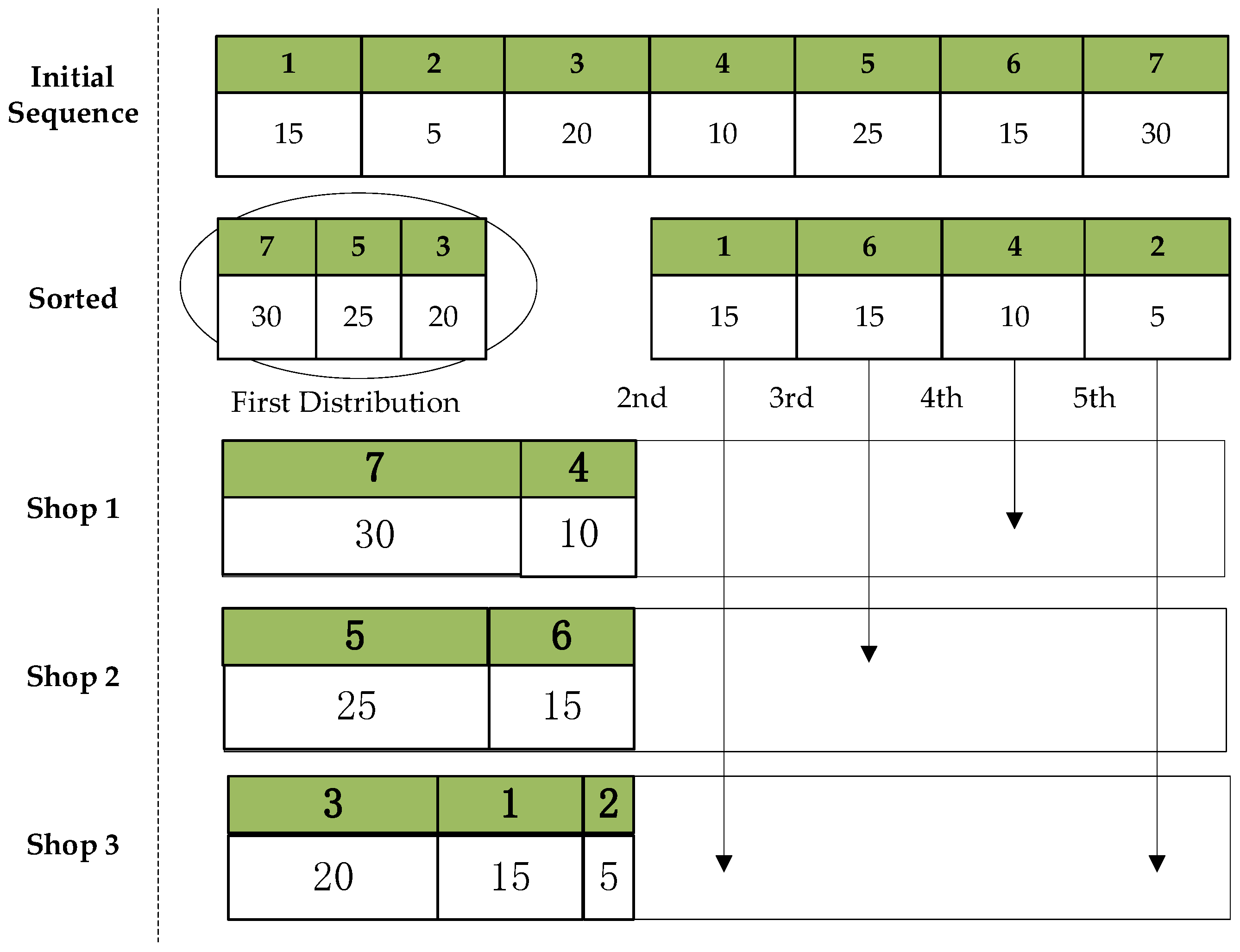
3.1. DPFSP Model Construction

Distributed System Architecture in Plant Simulation is a way to improve simulation efficiency by splitting the production process into multiple subsystems or computing nodes, especially for large, complex production systems. In this architecture, the production process is decomposed into multiple independent modules, each of which can run independently on different computer nodes, thus achieving faster computation speed and more efficient resource utilization. By coordinating multiple simulation modules and computing nodes, the distributed system significantly improves the simulation performance, especially when dealing with large-scale, multi-workshop, and complex production processes, thereby effectively reducing the computation time and resource consumption.

The dataset selected in this paper is the Taillard dataset, a benchmark instance data for the distributed replacement flow shop scheduling problem. Each factory in this dataset contains up to 20 machines, with a maximum of seven factories. The data specifications are shown in

Table 1. Results of ablation experiment.

Number of Workpieces	Number of Machines	Number of Workshops
20	5, 10, 20	2, 3, 4, 5, 6, 7
50	5, 10, 20	2, 3, 4, 5, 6, 7
100	5, 10, 20	2, 3, 4, 5, 6, 7
200	10, 20	2, 3, 4, 5, 6, 7
500	20	2, 3, 4, 5, 6, 7

below.

Firstly, the DPFSP is split into several sub-problems, and each sub-problem can be handled by a separate simulation module. Each workshop can be treated as an independent module, while task assignment, scheduling, and allocation of machine resources can be handled separately. The number of enabled workshops is selected by judging the input data type, and each module or subsystem is simulated on different computing nodes. Real-time data exchange and synchronization through the network can avoid the performance bottleneck of a single computing node. In this system, it is expanded to seven, as shown in Figure 4 below. In the DPFSP considered here, the number of machines as well as the production speed are identical across workshops. Thus, it is only necessary to determine the order of the combination of different machines as well as the number of machines assigned to each workshop. For each independent plant, a total of 20 machines are designed. The distribution of machines in the validated DPFSP model is illustrated in Figure 5 below.

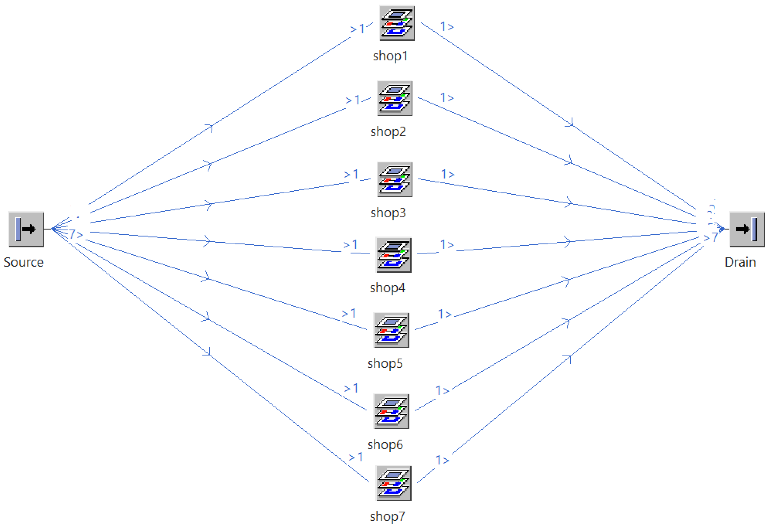
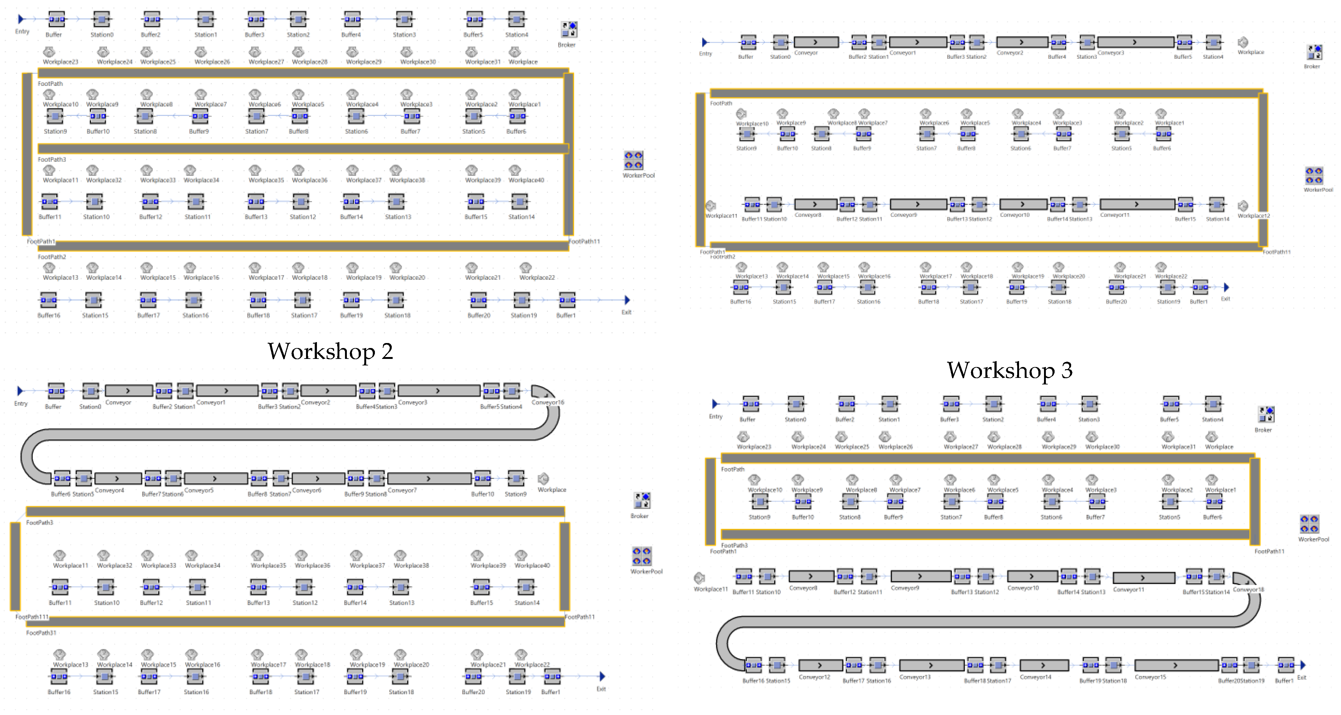
3.2. MSRDPFSP Model Construction

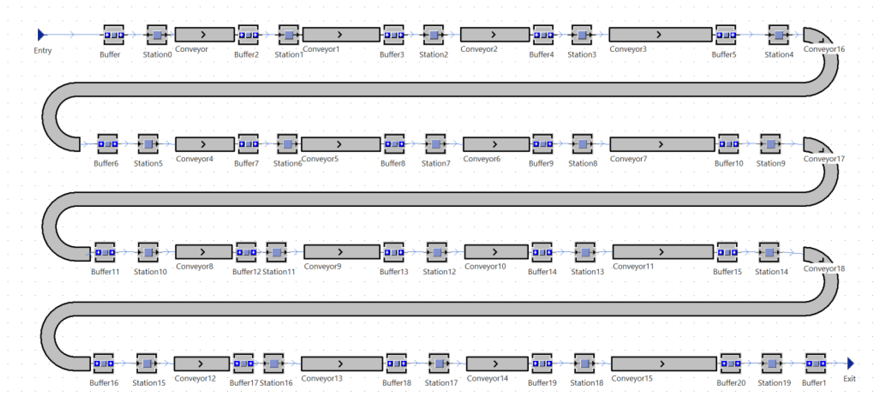
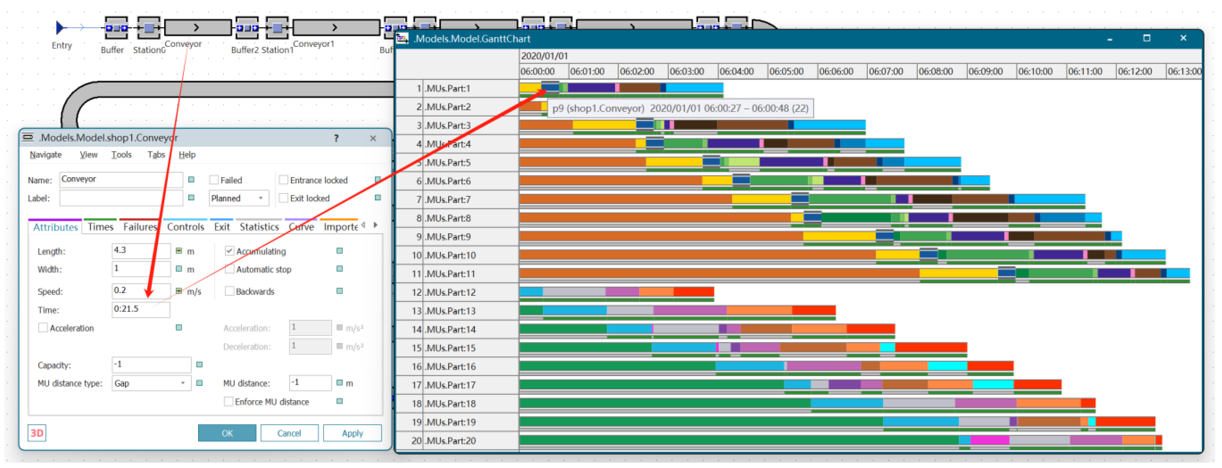
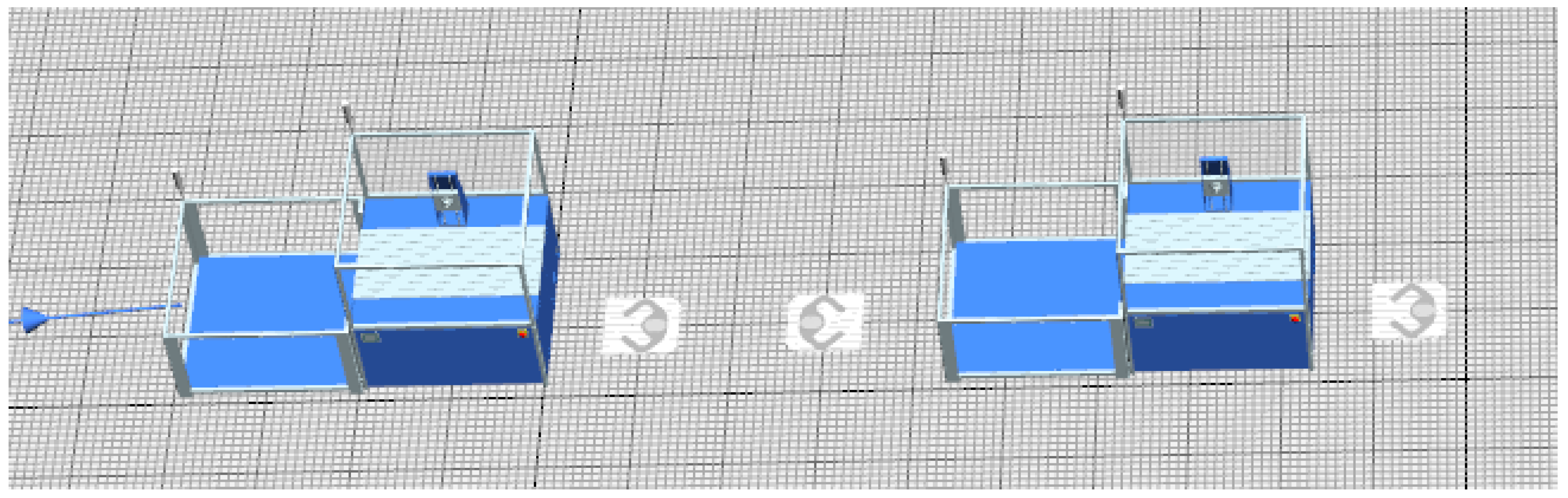
3.2.1. Conveyor Belt Workshop Construction

One of the assumptions of the DPFSP includes that the transfer time of the workpieces between the two processes is not counted. However, in practice, the material handling and transfer between the workshops may be a non-negligible part of the DPFSP, as the machining sequences of the DPFSP have already been determined. Therefore, it is particularly suitable for transporting the workpieces for the machines by means of a conveyor belt in the future, and the conveyor belt is one of the key elements for automation and optimization of the assembly line workshop. In Plant Simulation, the entire production process can be accurately simulated and optimized by setting the speed, capacity, path, and other parameters of the conveyor belt. The speed of the conveyor belt determines the speed at which the workpiece moves on the conveyor belt, and the capacity of the conveyor belt usually refers to the maximum number of pieces that can be transported at a time. Workpieces are transported between machines via a linear, irreversible conveyor belt. The conveyor belt cannot reverse until the processing task of the preceding machine is completed. The workpiece is stored in the buffer when the previous machine has not completed the machining task, as shown in Figure 6 below.

By setting the speed and length of the conveyor belt, the component automatically calculates the transfer time of the workpiece between different machines. Differences in calculations between the workshop in Figure 6 and the workshop in Figure 5 are shown in the Gantt chart in Figure 7 below.

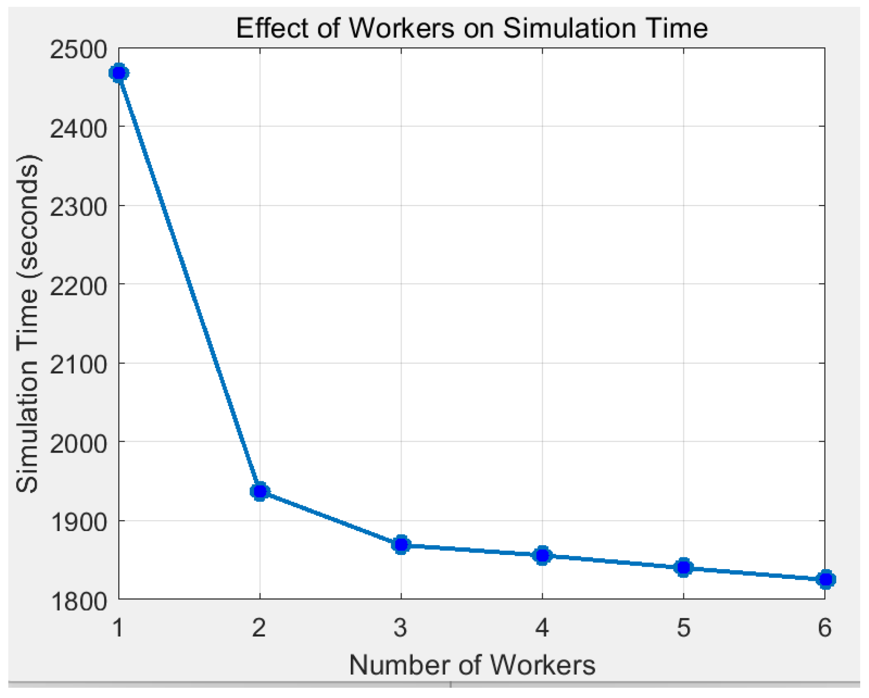
3.2.2. Workshop Construction for Workers

Workers are an important part of shop floor scheduling [37], requiring comprehensive consideration of multiple factors such as worker assignment, movement paths, task scheduling, and rest management [38]. Through reasonable modeling and optimization, the production efficiency can be improved, the waiting time of workers can be reduced, and the whole production system can thus be optimized. The WorkerPool can be considered a parallel computation manager responsible for distributing tasks among multiple worker threads. Compared to conveyor belts, when the number of workers on the shop floor is low, tasks should be queued for available workers, which can increase the time it takes for workpieces to flow within a certain range. Increasing the number of workers improves productivity. However, when the number of workers exceeds a certain threshold, the improvement in scheduling time decreases. Additionally, excessive complexity in worker scheduling may even reduce management efficiency, as shown in Figure 8 below.

The Worker object is linked to the production workstation to indicate that a certain worker performs a particular operation. Each workstation can have more than one worker resource to execute tasks, set the number of workers, and assign tasks to the workers. The WorkerPool component specifies the number of workers assigned to each workstation and the working and rest time of the workers, etc. The WorkerPool can be regarded as a parallel computing manager, responsible for allocating tasks among multiple worker threads. When the number of workers in the workshop is small, tasks need to queue up and wait for available workers, which leads to an increase in the flow time of the workpiece within a certain range. Increasing the number of workers can improve productivity. However, when the number of workers exceeds a certain threshold, the improvement effect of scheduling time declines, and even the management efficiency may decrease due to overly complex worker scheduling. Details are illustrated in Figure 9 below.

Upon completing the basic resource allocation, it is necessary to create a Path according to the layout of the workstations to reasonably connect the workstations with the starting points of the workers and form a complete walking route network. Combined with the SimTalk scripting language, it can also achieve a high degree of customization of worker behaviors, such as task assignment, path selection, waiting mechanism, etc., so as to achieve complex production scheduling strategies and path optimization during the simulation process. This also provides strong support for modeling a variety of production systems. In combination with the assembly line shop, six additional shops are constructed, as shown in Figure 10 below.

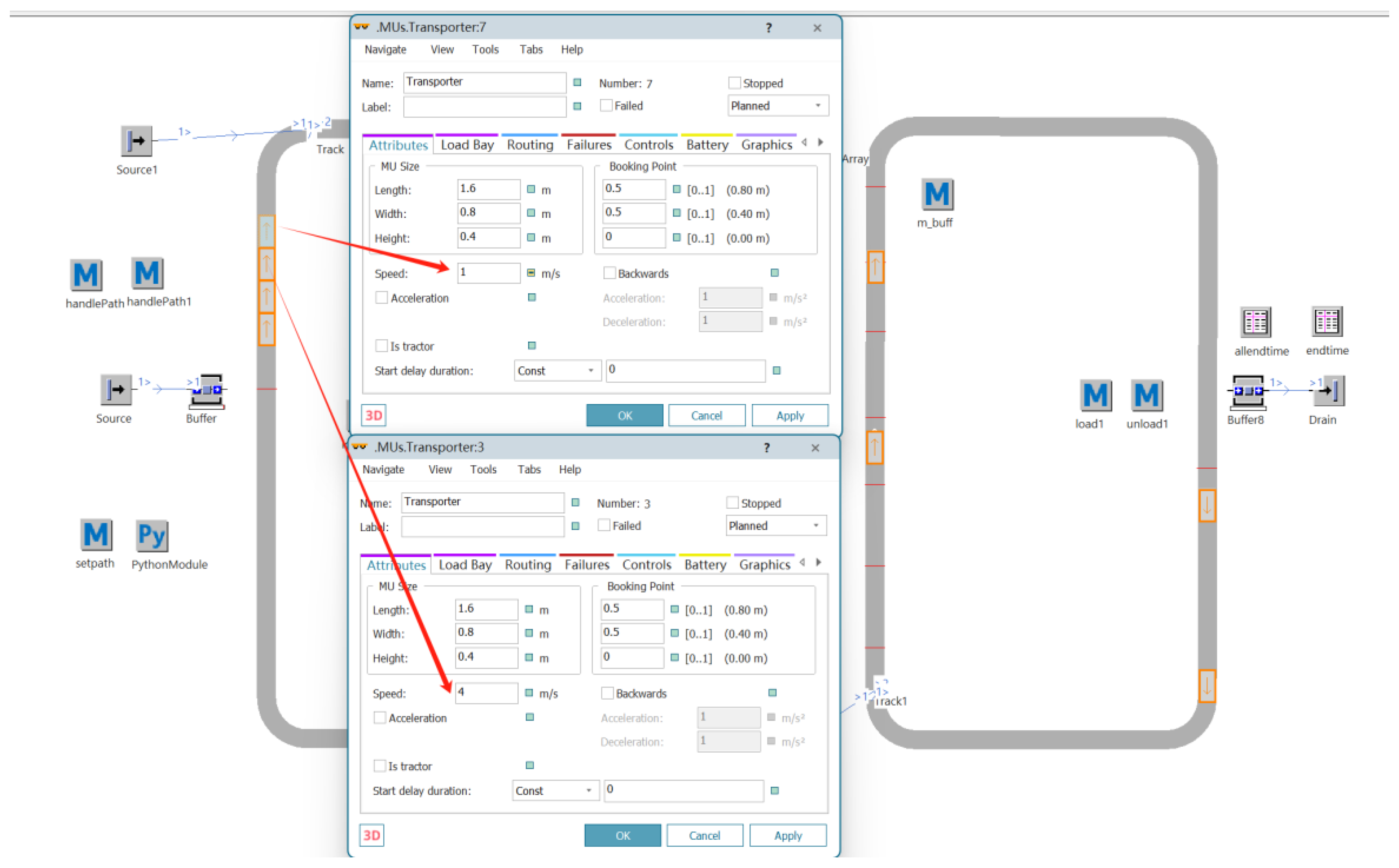
3.2.3. AGV Carts and Robotic Arms and Path Setting

With the advancement of logistics automation, workshop logistics transportation tools forklifts and rickshaws are gradually replaced by AGVs. Since the price of AGV is generally in the hundreds of thousands of dollars, the reasonable number of AGVs and the design of logistics routes have become key considerations in the design of automated workshop logistics [39]. To address this problem, a distributed system with AGV carts and robotic arms is constructed to simulate the collaborative work of AGVs and robotic arms, and to ensure the efficient operation of the system by means of a scheduling system, path planning, etc. The paths of AGV carts constitute a critical factor in determining their movement patterns within a factory or production environment [40]. In this paper, preset paths, which are usually defined through node objects and connecting lines, are used. The AGV will move in the order between these path points. This paper does not consider the problem of path optimization but introduces this component to simulate machine logistics and replicate a multi-scenario shop floor environment. As illustrated in Figure 11 below, the path is configured as a circle track to facilitate the flow of the whole system. The sensors on the track are used to detect the position and status of AGV (Automated Guided Vehicle), other transportation equipment, and the items passing through the position. When an AGV traverses a node, these sensors are triggered. As an important part of the intelligent logistics system, the track-mounted sensors enable precise detection of transporters or AGVs’ positions, facilitating dynamic path control, obstacle avoidance, task triggering, and data analysis. The workpieces are transported to the sensors via AGV carts and then transported to individual workshops via PickAndPlace.

The simulation time of MSRDPFSP workshop is affected by many conditions, such as the number and speed of AGV carts, whether the transportation path is blocked or not, the loading time and unloading time of the robotic arm, etc. Each will affect the final simulation time. The parameters of the Transporter need to be set reasonably. Similar to the allocation of workers across workshops, the number of AGV carts directly affects the final simulation time. The speed of each Transporter and other information also matter considerably. If a cart runs too slowly, it will lead to congestion in the entire AGV system along its path. As shown in Figure 12 below, when the speed of one of the carts is 1 m/s and the time of other carts is 4 m/s, such speed discrepancies lead to system-wide blockages.

The difference between the first two parts is that when the workpieces enter each workshop, they need to be delivered by the AGV carriage to the buffer of the robot arm and wait for the robot arm to deliver the workpieces to each workshop.

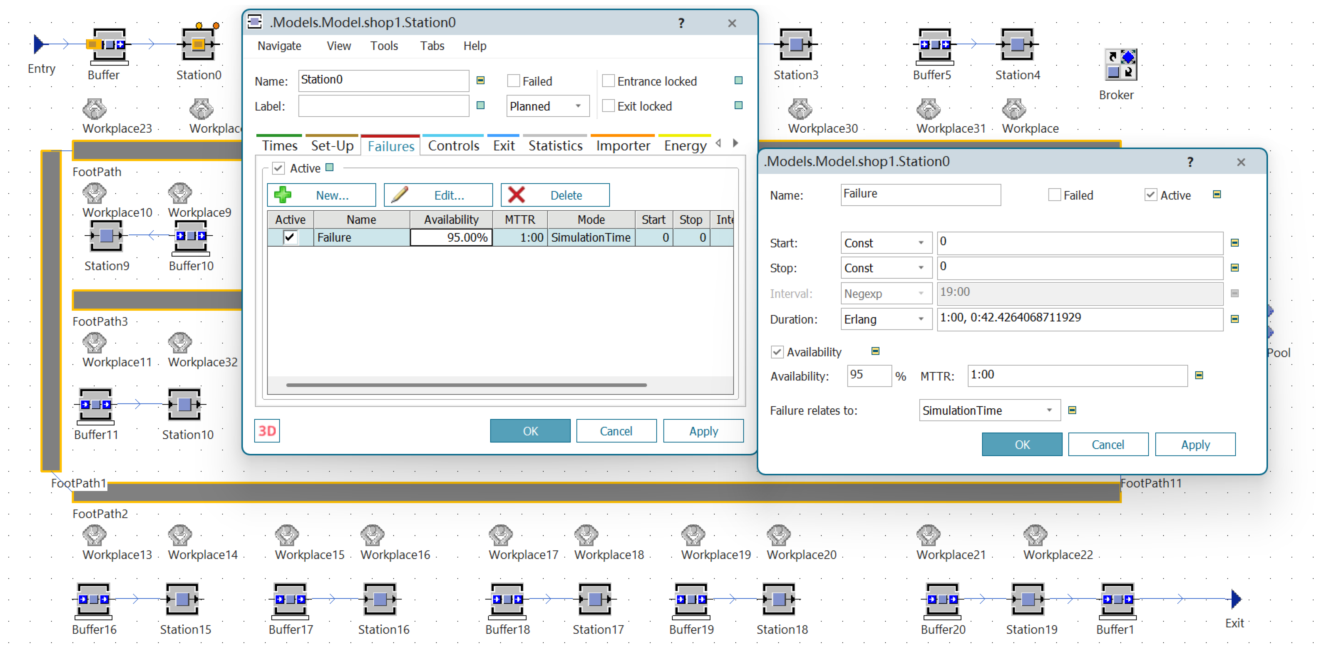
3.2.4. MTTR and Statistics Function Settings

Mean Time to Repair (MTTR) plays a crucial role in production scheduling, and its value directly affects equipment availability [41], scheduling stability, and overall productivity. In order to more realistically simulate the reliability characteristics of the equipment in actual production, the failure behavior and MTTR are configured for each machine and equipment, as shown in Figure 13 below. Through this configuration, equipment in the simulation will exhibit periodic failure and repair patterns following statistical laws, thereby influencing the overall scheduling process. This design aligns the scheduling model with the uncertainty characteristics of real-world production systems, thus enhancing the robustness of the model analysis capabilities.

Upon setting the faults of the equipment, in order to ensure that the fault occurrence and maintenance behavior of the equipment can be correctly executed in accordance with the preset random pattern at the beginning of each simulation or the initialization of each round of the production task, the reset random variable is set in the EventController. Consequently, the random distribution related to the faults is re-initialized at the beginning of the simulation, avoiding the repetition or distortion of the simulation results due to fixed random seeds. This improves the accuracy and realism of the simulation, which is especially important in the comparison of multiple experiments or robustness analysis, as shown in Figure 14 below.

3.2.5. Statistical Modules and Summaries

In the Drain module, by setting the SimTalk script function, it accurately records the time when each workpiece finishes processing and leaves the system. Concurrently, it tags the workpiece with its originating workshop and its completion sequence within that workshop. Based on this recording mechanism, real-time statistics on the completion of each workpiece in each workshop can be achieved. Specifically, the time when the last workpiece exits each workshop is extracted as the makespan of the workshop. The makespan of each workshop effectively captures the load distribution and production bottleneck information of each workshop during the scheduling process, reflecting not only the operational pressure within individual workshops but also revealing the overall efficiency of system resource utilization and coordination levels. Makespan as a feature input can provide richer and more meaningful state information for the subsequent reinforcement learning algorithms. This can help the intelligentsia accurately perceive the actual impacts of different scheduling schemes on the system performance, optimizing the resource allocation and job sequencing more efficiently during the decision-making process, and improving the convergence speed and policy quality of the learning.

The introduction of assembly lines as well as workers introduces workpiece transfer time between stations, thereby increasing the computational complexity on the shop floor. The incorporation of AGV trolleys, paths, and robotic arms introduces time costs for workpiece distribution, thereby elevating the computational complexity off the shop floor. The first three parts are the embodiment of multi-scenarios. In each simulation, the same scheduling sequence remains consistent across scenario changes, while the introduction of failure rates leads to different simulation results for the same sequence, which embodies the model robustness.

4. Algorithm Design

4.1. Search Strategy

The quality of the initial solution plays a crucial role in the training performance of reinforcement learning algorithms. In the DDQN algorithm, the intelligent body continuously optimizes its strategy by interacting with the environment, and the quality of the initial strategy directly affects the convergence speed of the learning process and the final scheduling performance; if the initial solution is of poor quality, the intelligent body needs a longer training time to explore a high-quality scheduling strategy, resulting in poor strategy convergence performance [42]. This paper addresses the MSRDPFSP by using the excellent initial solution generated based on the NEH algorithm as the policy starting point of the DDQN intelligences and performing continuous iterative learning in a multi-scenario, dynamic uncertainty environment. Although there are some differences between DPFSP and MSRDPFSP in terms of problem complexity and scenario diversity, the experimental results show that the initial solution generated by NEH can significantly outperform the completely random initialization in the robust optimization process. For this initial solution, the following four global search strategies are designed:

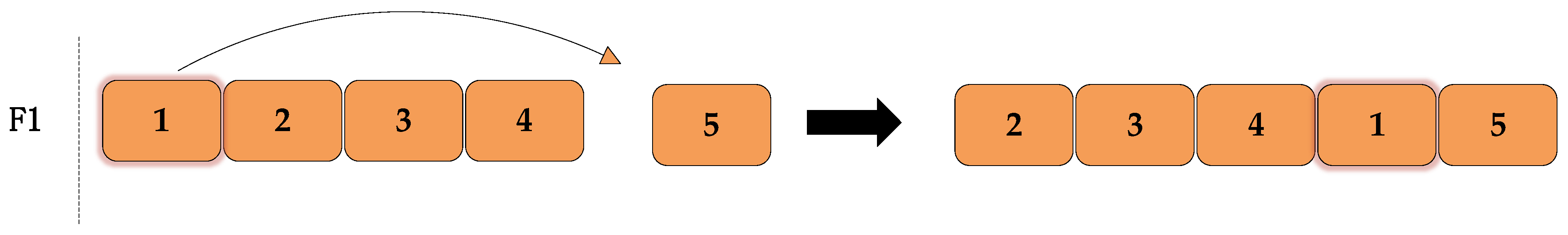
• Insertion within workshop: It is executed for all workshops. A set of consecutive sequences within a workshop are randomly selected and inserted into a random position in that workshop. If there is optimization, the optimized sequences are returned; otherwise, the pre-optimized sequences are returned, as shown in Figure 15 below.
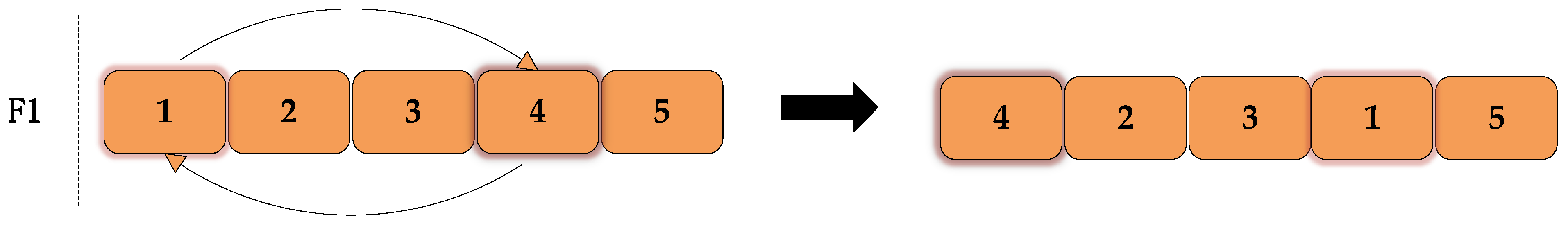
• Intra-workshop swapping: It is executed for all workshops. A set of consecutive sequences within a workshop are randomly selected to recombine their positions, and the optimized sequence is returned if there is an optimization; otherwise, the pre-optimized sequence is returned, as shown in Figure 16 below.
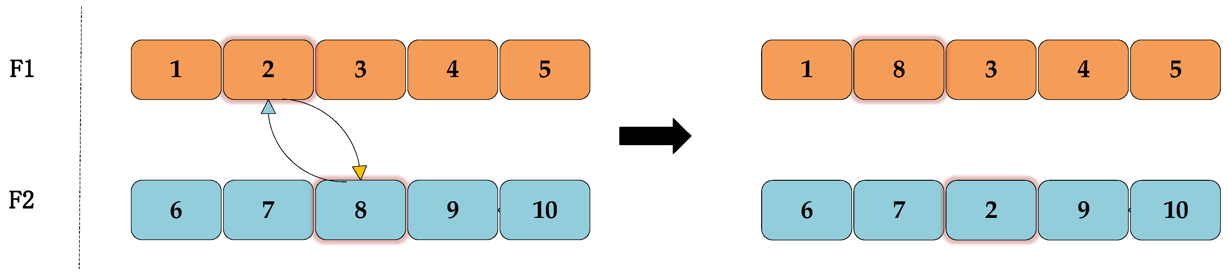
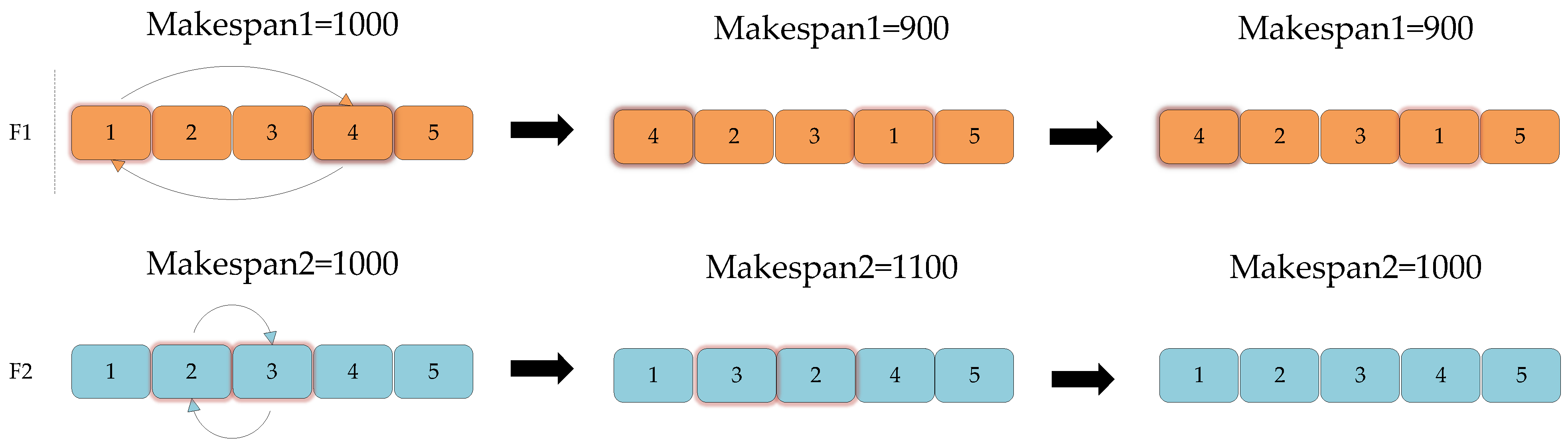
• Swap between different workshops: All workshops are sorted in terms of elapsed time. Specifically, a set of consecutive sequences in the workshop with the longest elapsed time are chosen to be swapped with the same number of consecutive random sequences in another random workshop. If there is an optimization, the optimized sequences are returned; otherwise, the pre-optimized sequences are returned, as shown in Figure 17 below.
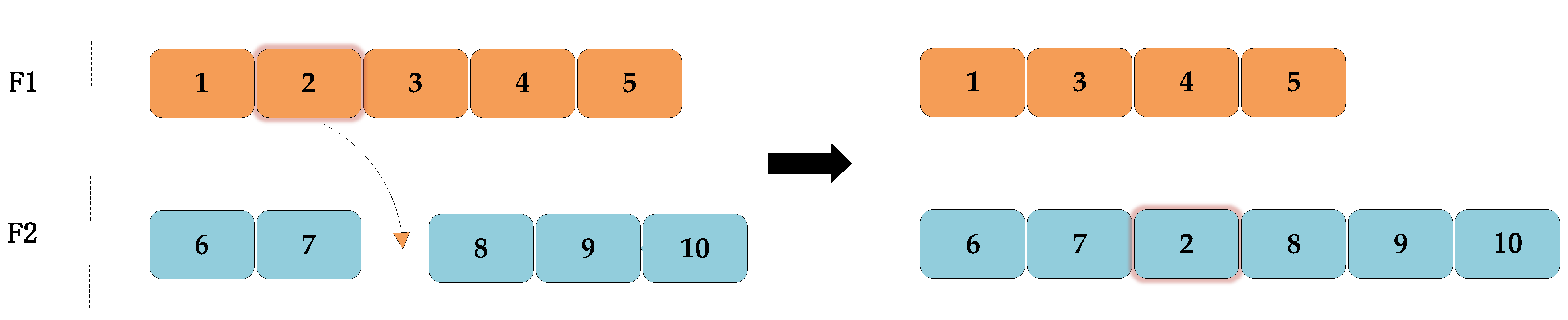
• Insertion between different workshops: All workshops are sorted in terms of elapsed time. Multiple tasks within the workshop taking the longest time are selected and inserted into other workshops with a short elapsed time. If there is an optimization, the optimized sequence is returned; otherwise, the pre-optimized sequence is returned, as shown in Figure 18 below.

In this paper, four local search strategies are set up for the insertion and exchange within the workshop. Different workshops do not affect each other. Compared with the traditional genetic algorithm, this approach only needs to interact with the simulation model once to make an optimization attempt for all workshops, as long as there is an improvement within the workshop. Even if there is no improvement in other workshops, the update sequence of the improved workshop is retained, while unimproved workshops continue to use their original sequence. This approach—retaining updates for improved workshops and maintaining original sequences for unimproved ones—is referred to as local updating in this paper, as shown in Figure 19 below.

For swapping between different workshops, both scheduling strategies target the workshop with the longest and shortest time consumption compared to the traditional method. This can quickly equalize the load of each workshop, and the neural network can extract more effective information.

4.2. Reward Function and Update Strategy Design

In the complex workshop scheduling environment, the state space is huge, and the uncertainty factor is significant. If the reward function design is unreasonable, it is easy to cause the learning direction of the intelligent body to deviate from the target [43], resulting in unstable or even invalid scheduling strategy generated. In the multi-scene DPFSP, the reward function design is as follows:

$$\begin{array}{c}\mathrm{r}\mathrm{e}\mathrm{w}\mathrm{a}\mathrm{r}\mathrm{d}=\left\{\begin{array}{c}5, \mathrm{O}\mathrm{v}\mathrm{e}\mathrm{r}\mathrm{a}\mathrm{l}\mathrm{l} \mathrm{i}\mathrm{m}\mathrm{p}\mathrm{r}\mathrm{o}\mathrm{v}\mathrm{e}\mathrm{m}\mathrm{e}\mathrm{n}\mathrm{t}\mathrm{s}\\ 3, \mathrm{l}\mathrm{o}\mathrm{c}\mathrm{a}\mathrm{l} \mathrm{i}\mathrm{m}\mathrm{p}\mathrm{r}\mathrm{o}\mathrm{v}\mathrm{e}\mathrm{m}\mathrm{e}\mathrm{n}\mathrm{t}\\ -1, \mathrm{u}\mathrm{n}\mathrm{i}\mathrm{m}\mathrm{p}\mathrm{r}\mathrm{o}\mathrm{v}\mathrm{e}\mathrm{d}\end{array}\right.\end{array}$$

(1)

For the MSRDPFSP with included fault rates, the same set of sequences will yield different results in this problem for different times of simulation. In order to improve the performance of DDQN in this problem, this study constructs a reward mechanism based on the ordering. This involves running three times of interaction between each set of scheduling sequences and the simulation model, then arranging the final results in ascending order, marking them as superior, medium, and inferior values in order, and making a comparison. The three sets of results corresponding to the old and new states are compared to obtain three sets of reward values. Finally, the weighted reward values are calculated as follows:

$$\begin{array}{c}\mathrm{r}\mathrm{e}\mathrm{w}\mathrm{a}\mathrm{r}\mathrm{d}=0.4 \times \mathrm{e}\mathrm{w}\mathrm{a}\mathrm{r}{\mathrm{d}}_{\mathrm{best}}+0.2 \times \mathrm{r}\mathrm{e}\mathrm{w}\mathrm{a}\mathrm{r}{\mathrm{d}}_{\mathrm{medium} }+0.4 \times \mathrm{e}\mathrm{w}\mathrm{a}\mathrm{r}\mathrm{d}\_\mathrm{w}\mathrm{o}\mathrm{r}\mathrm{s}\mathrm{t}\end{array}$$

(2)

The convergence effect of the three-valued sorting algorithm under the MSRDPFSP is shown in Figure 20 below. The update strategy is set to perform population replacement only when the total value improves and the other logics are kept unchanged. In order to enhance the exploratory ability and convergence efficiency of the DDQN in solving the MSRDPFSP, a dynamically adjusted greedy rate strategy is designed in this study. The initial greedy rate (ε) is set to 1 to ensure that the intelligent body has sufficient exploratory ability in the early stage of training; with the advancement of training, the greedy rate gradually converges at a rate of 0.2% reduction per iteration round until it is reduced to 0.1. Meanwhile, in order to avoid the exploratory ability loss of new strategies in scenarios of local optimums or training stagnation, when the successive reward obtained is less than or equal to 0 (indicating no improvement in scheduling performance), the greedy rate is increased by 0.1% each time. This adjustment restores the exploration ability of the intelligent body, thus improving the probability of jumping out of the local optimum.

4.3. DDQN Neural Network Design

For the MSRDPFSP, since it belongs to the NP-hard problem in combinatorial optimization, the state space is extremely large, and it is not feasible to record all the q-values corresponding to all the states at one time. For the data of 500 workpieces assigned to seven workshops, there are 7500 possible solutions, and such a state–action mapping cannot be stored or trained. Therefore, it is necessary to rely on function approximation methods, such as neural network structures common in DQN for approximate representations, to dynamically learn the value functions of state–action pairs.

If the state is stored by means of the traditional gene chromosome, for the data of 500 workpieces, the dimension of state is 1000. Given that the gene chromosome cannot obtain the specific processing time of each workpiece on each machine, the information that can be extracted is also limited. Consequently, in this paper, the information stored in the state is the makespan value of each workshop. Given the presence of failure rates and processing time uncertainty in the problem model, a set of sequences interacts with the model three times to generate results that collectively form the state information. This state information is solely tied to the number of workshops; for seven workshops, the dimensions of the state is only 21, compared to just 7 in a model without failure rates. This greatly reduces the training difficulty. Moreover, makespan can more intuitively express the state information of each workshop, and the information stored by the neural network each time is shown in Figure 21 below.

4.4. Joint Communications Establishment

4.4.1. Joint Calls Via COM Interfaces

Win32com is a Python-based COM interface library [44]. It enables Python scripts to call COM-enabled application objects on Windows platforms as clients, realizing cross-software data interaction and process control [45], thereby dynamically scheduling the simulation process and collecting real-time system state data without relying on the traditional graphical interface operation. Through this mechanism, the DDQN algorithm can directly manipulate the simulation model while batch generating and evaluating the performance index of different scheduling schemes, which greatly improves the automation and computational efficiency of the scheduling optimization process. Compared with the traditional manual modeling and validation, the combination of Python and Plant Simulation simplifies the complexity of the model control. Concurrently, it also enables the scheduling algorithm to be flexibly migrated to different types of workshop simulation models, reflecting the high ease of use, versatility, and value of engineering applications. Details are shown in Figure 22 below.

The time management component of Plant Simulation is the EventController. Through EventController, the simulation speed of the model can be set. Prior to the simulation, the simulator should be reset using the Reset function. The startWithoutAnimation function is used to initiate the simulation. The difference between startWithoutAnimation and start is that startWithoutAnimation directly ignores all dynamic processes, enabling the model to obtain the simulation results at full speed. This is also the main bottleneck in the current experimental process. Even with full-speed simulation, the model will still be affected by the complexity of the model. As the problem scale expands, the simulation time will increase significantly.

Table 2. Time consumed at different data sizes.

N × M × F	Time	N × M × F	Time
100 × 5 × 7	0.03 s	100 × 5 × 2	0.03 s
100 × 10 × 7	0.04 s	100 × 10 × 2	0.04 s
100 × 20 × 7	0.04 s	100 × 20 × 2	0.06 s
200 × 10 × 7	0.05 s	200 × 10 × 2	0.06 s
200 × 20 × 7	0.08 s	200 × 20 × 2	0.11 s
500 × 20 × 7	0.18 s	500 × 20 × 2	0.26 s

below shows the time required for one simulation of the model at partial scale. After each simulation is initiated—where N represents the number of workpieces, M represents the number of machines, and F represents the number of workshops—it is necessary to wait for the simulation to conclude before using the GetValue function to retrieve the simulation results of the model. The ExecuteSimTalk function is used to execute SimTalk script functions and control all behaviors, variables, and parameters in the model.

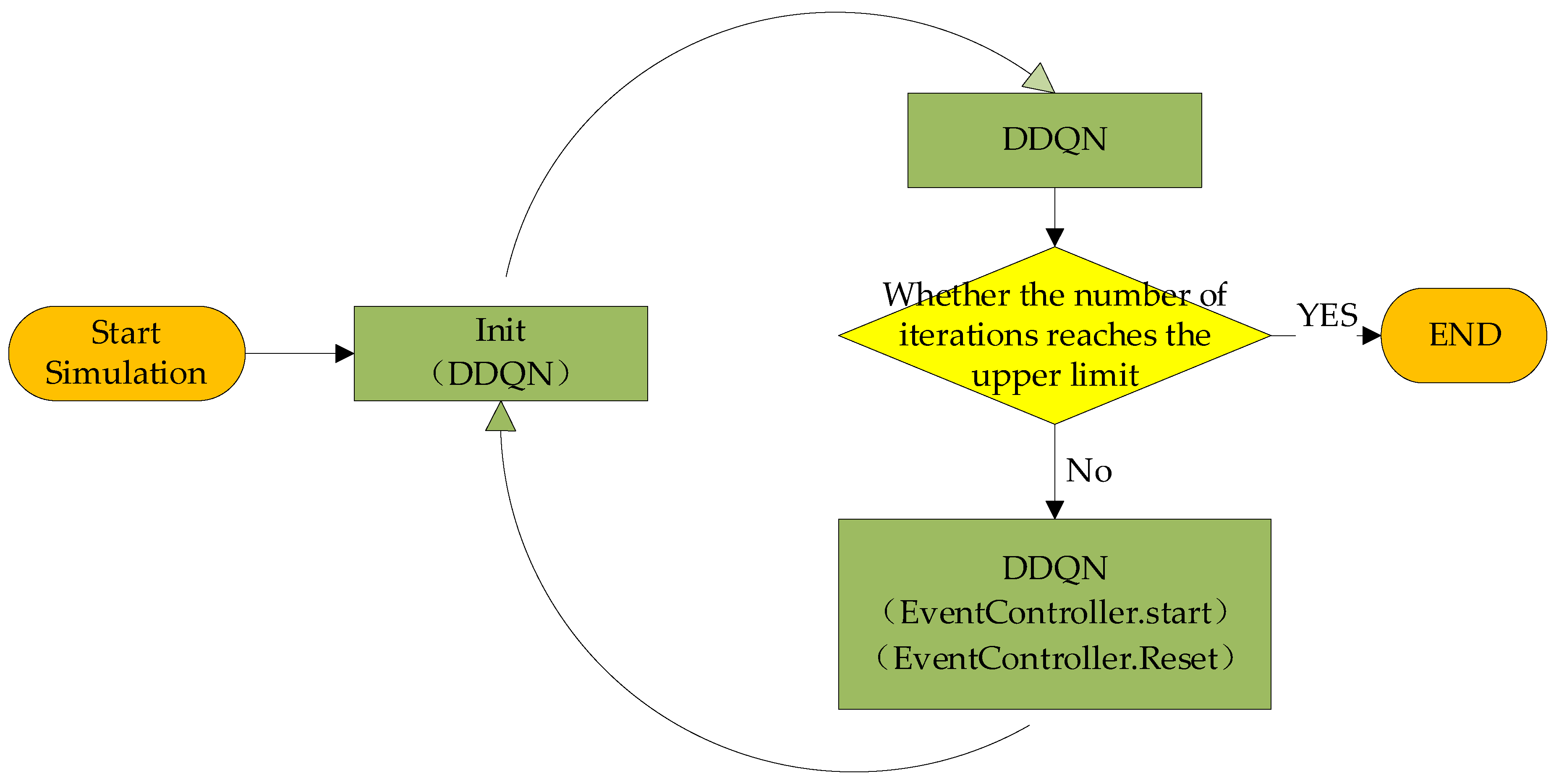
4.4.2. Joint Calls Via DLL

Since version 24.04, Plant Simulation has supported direct interaction with simulation models using Python, with the minimum version being 3.12. Before calling, the setPythonDLLPath function is first used to allocate the DLL path address for Plant Simulation [46]. Plant Simulation itself has a built-in time manager. If the time controller is manually run too many times, errors may occur. To achieve the same continuous iterative effect as the COM interface, the solution adopted in this paper is to place the DDQN component in the init function. The init function is used to initialize the parameters, variables, and objects of the model before the simulation starts. This ensures that the simulation is carried out in the correct initial state. Each time this function is executed, the event manager will be reset, as shown in Figure 23 below.

4.5. Algorithm Flow

Firstly, the initial population is generated by the NEH algorithm. Meanwhile, the joint simulation system of the DDQN algorithm and the MSRDPFSP model is constructed, and the heuristic optimization iterations are continuously performed on the initial population through four scheduling strategies. As the number of iterations continues to improve, the intelligent agent gradually learns to select scheduling strategies with a larger solution space. The specific flow of the algorithm is shown in Figure 24 below.

5. Experiments

5.1. DDQN Performance Evaluation for DPFSP

The experimental platform configuration consists of an Intel 13900k CPU @3.0 GHz and a NVIDIA GeForce RTX 4080 (16 GB) GPU running on the Windows 11 operating system with PyTorch 2.4.1 deep learning framework, CUDA 12.4, and Python 3.13. Plant Simulation uses Version 24.04.

To further evaluate the superiority of the DDQN algorithm proposed in this paper, the percentage deviation RPD is employed to measure the superiority of the algorithm and is calculated as:

$$\begin{array}{c}\mathrm{R}\mathrm{P}\mathrm{D}={\displaystyle \frac{\mathrm{Alg} - \mathrm{Min}}{\mathrm{Min}}}\times 100\end{array}$$

(3)

where Alg denotes the best maximum completion time for both algorithms, and Min denotes the best minimum completion time found in the benchmark example Taillard dataset. The validation is carried out through different combinations of the number of artifacts and the number of machines in the dataset, as each combination has 10 different iterations of the algorithm, which is very computationally intensive. Therefore, in this paper, ARPD is used to denote the average RPD of the same combination in different repetitions, and the formula is as follows. The final results are shown in

Table 3. Model elements and their names commonly used in Plant Simulation software.

N × M × F	DDQN	NEH	N × M × F	DDQN	NEH
100 × 5 × 2	0.74	7.24	200 × 10 × 2	0.86	6.12
100 × 5 × 3	0.50	5.43	200 × 10 × 3	1.85	6.93
100 × 5 × 4	0.38	4.41	200 × 10 × 4	1.91	5.82
100 × 5 × 5	1.35	7.80	200 × 10 × 5	1.91	5.54
100 × 5 × 6	1.71	7.83	200 × 10 × 6	2.28	5.60
100 × 5 × 7	1.32	6.24	200 × 10 × 7	2.60	5.11
100 × 10 × 2	0.72	5.15	200 × 20 × 2	0.29	5.28
100 × 10 × 3	1.93	6.87	200 × 20 × 3	0.08	2.83
100 × 10 × 4	2.14	6.31	200 × 20 × 4	0.08	1.84
100 × 10 × 5	1.89	5.69	200 × 20 × 5	1.62	8.17
100 × 10 × 6	2.52	6.06	200 × 20 × 6	1.84	7.91
100 × 10 × 7	2.34	4.95	200 × 20 × 7	1.23	6.26
100 × 20 × 2	0.73	6.67	500 × 20 × 2	0.84	6.40
100 × 20 × 3	0.17	3.31	500 × 20 × 3	2.10	6.86
100 × 20 × 4	0.19	3.89	500 × 20 × 4	1.81	6.03
100 × 20 × 5	1.36	7.88	500 × 20 × 5	1.95	5.93
100 × 20 × 6	1.52	7.34	500 × 20 × 6	2.39	5.38
100 × 20 × 7	1.26	5.67	500 × 20 × 7	3.03	5.13

below, where N represents the number of workpieces, M represents the number of machines, and F represents the number of workshops. Other parameters of DDQN are shown in

Table 4. DDQN parameter setting.

Parameters	Hidden Meaning	Parameter Value
lr	Discount rate	0.005
batch_size	Number of training samples	32
EPSILON	Initial greedy rate	1
EPSILON_decay	Decay rate	0.998
EPSILON_min	Minimum greedy rate	0.1
GAMMA	Discount rate	0.9
TARGET_REPLACE_ITER	Synchronization frequency	16
MEMORY_CAPACITY	Experience pool size	128

below.

$$\begin{array}{c}\mathrm{A}\mathrm{R}\mathrm{P}\mathrm{D}={\displaystyle \frac{{\sum }_{\mathrm{i}=1}^{10}{\mathrm{RPD}}_{\mathrm{i}}}{10}}\end{array}$$

(4)

Through data analysis, the introduction of the NEH and DDQN algorithms endows the DPFSP with a better performance at the initial stage under different numbers of workpieces and plant sizes. Through continuous iterations, 121 groups out of 720 groups of data can reach the optimal value and show better ARPD values, which verifies the effectiveness of the algorithms proposed in this paper.

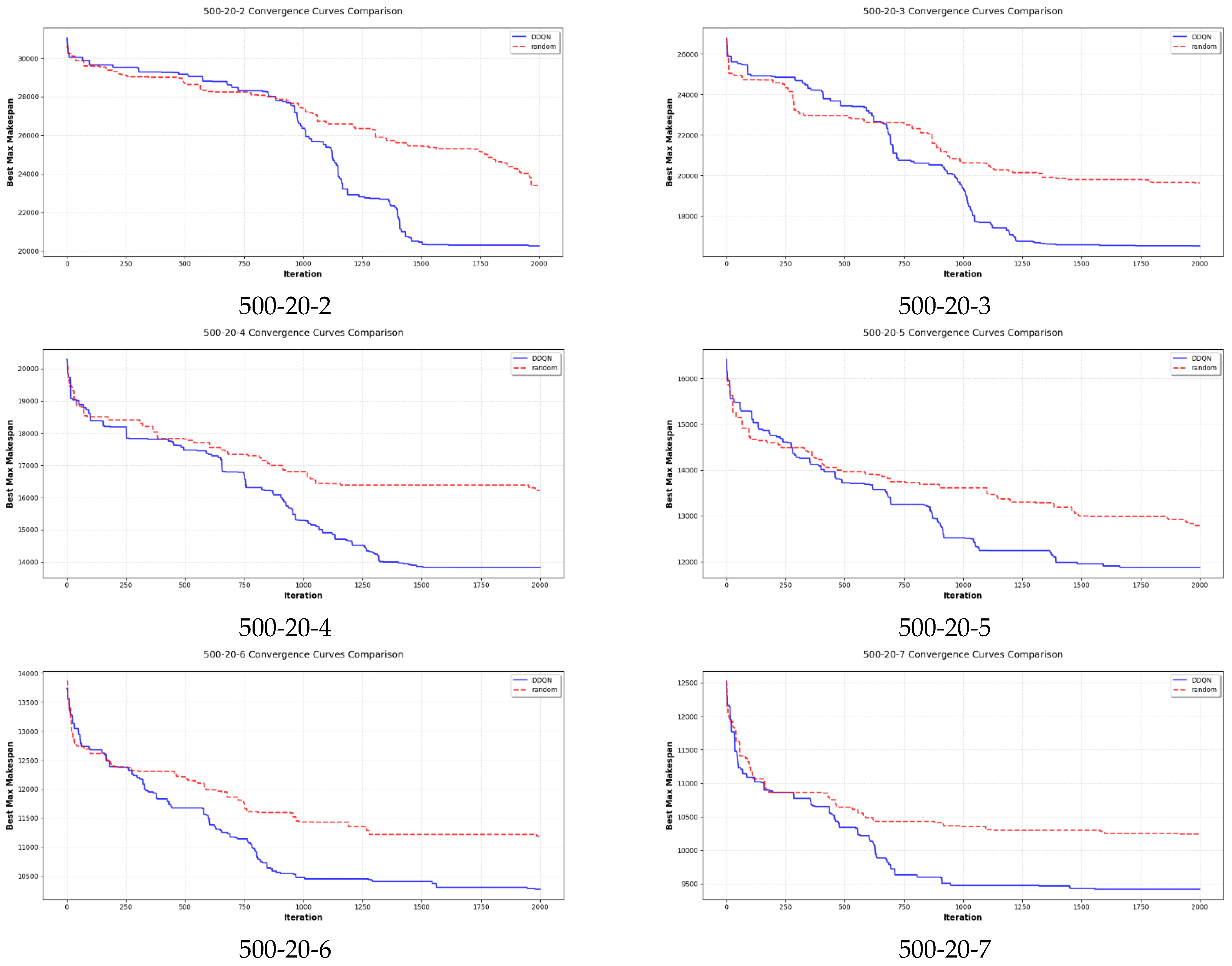
5.2. DDQN Performance Evaluation for MSRDPFSP

Since there is no publicly available dataset for testing MSRDPFSP, the publicly available dataset of DPFSP is still used. The dataset mainly tests the data of 500 workpieces processed by 20 machine tools allocated to different workshops. The convergence curves of the random search strategy algorithm and the DDQN algorithm with 2000 iterations are compared. The test results are shown in Figure 25 below.

From the convergence curve, it can be seen that after the introduction of the DDQN algorithm to learn the strategy, it shows faster convergence speed and better results compared to the random selection strategy during the iteration process. Specifically, once the experience pool has accumulated enough experience and gradually starts to select from randomly selected actions to high q-value actions, the convergence speed of DDQN starts to be significantly ahead of the randomly selected algorithm. This empirical superiority underscores DDQN’s capacity to effectively guide the scheduling policy to converge towards the optimization goal and highlights its enhanced learning ability and optimization performance for the MSRDPFSP with uncertain processing times.

Taking the data of 500-20-7 as an example, the initial solution of NEH for the DPFSP in MSRDPFSP each workshop is initially not balanced. Workshop 1 has a faster machining speed because of the use of conveyor belts in the workshop. Over 2000 iterations, the stochastic optimization strategy distributes scheduling actions nearly uniformly (approximately 500 executions per strategy), whereas the DDQN algorithm selectively executes the insertion strategy 800 times after learning its higher reward potential. Specifically, DDQN prioritizes inserting workpieces from the longest-processing-time workshop into the shortest-processing-time one. This learning does not take too much time: the time taken for executing the DDQN strategy for the 2000th time is 1025 s, while that of the stochastic strategy is 1000 s, as shown in Figure 26 below.

Plant Simulation has a built-in genetic algorithm component for the workshop scheduling problem, which is compared with the hybrid algorithm proposed in this paper, using the same data, with the initial population size set to 20, 100 iterations, and a final elapsed time of 1000 s. The results obtained are shown in Figure 27 below. As illustrated in the figure, the experimental comparison demonstrates that the approach proposed in this paper outperforms the hybrid algorithm, which in turn significantly surpasses this genetic algorithm module.

6. Discussion

Distributed systems are essentially designed to cope with the limitations of a single system or plant difficult to meet complex demands. This idea is applicable in several fields, including intelligent scheduling in manufacturing, computer system architecture, and data processing. In intelligent manufacturing and shop scheduling problems, with the complexity of the production environment, it is difficult to manage all tasks efficiently with only a single software or centralized system. As a result, distributed scheduling and co-simulation have become prominent trends, with different software or system modules each playing distinct roles. Broadly speaking, distributed is not only a trend in the manufacturing industry, but also a direction for the development of the entire intelligent society.

In this article, the method of calculating the scheduling sequence time is obtained by interacting with the simulation model to obtain simulation results. This method demonstrates significant advantages in reproducing real and complex production environments. The hybrid algorithm proposed in this article can efficiently perform heuristic optimization within the black box environment of this interactive simulation system. However, it also entails several limitations, detailed as follows:

Firstly, the calculation of such results is limited by the model’s maximum speed for obtaining simulation results, which far exceeds the neural network’s learning time. To address this, this paper employs a lot of operations to improve efficiency, yet at the expense of the diversity of the initial population.

Secondly, the computation of a new scheduling sequence must wait for the end of the last simulation to start. If a new scheduling sequence is introduced before the simulation concludes, the simulation will terminate early, yielding an erroneously smaller value for that scheduling sequence. Consequently, subsequent optimizations of the sequence of the altered group cannot exceed the wrong value, causing the algorithm to become trapped in a wrong local optimum.

Thirdly, in this kind of iterative problem, despite the time saved by using DLL calls between Plant Simulation and Python compared to COM interface calls, this approach still has significant limitations. Notably, when using the COM interface in Pycharm, the simulation model can run without opening the simulation software’s interface, which enables the fastest and most stable simulation performance.

7. Conclusions

For the MSRDPFSP, which is difficult to be modeled by traditional simulation methods, this paper employs Plant Simulation to digitally model MSRDPFSP using a hybrid algorithm of DDQN and NEH, and heuristically interacting with the simulation model through the COM interface and DLL. The experiments show that the DDQN algorithm can well guide the intelligences to choose the model with higher return values and better robustness. Moreover, the hybrid algorithm achieves far better results than the genetic algorithm component of Plant Simulation in a shorter time, verifying the advantages of the co-simulation system in this paper. For the first time, the MSRDPFSP is combined with the DDQN algorithm and the Plant Simulation software of Siemens. Overall, this offers a novel perspective for addressing problems that require consideration of complex mathematical modeling, data analysis, and high-performance computing.

Due to the limited conditions, the construction of the model in this paper relies on the Taillard dataset of the DPFSP rather than the construction of the real production workshop environment. Thus, it cannot be called a digital twin workshop. In the future, integration with more complex and dynamic real-world production environments should be considered. It is anticipated that such a joint simulation system will assume a more pivotal role in the field of digital twin workshops.

References

1. Ghobakhloo, M. Industry 4.0, digitization, and opportunities for sustainability. J. Clean. Prod. 2020, 252, 119869. [Google Scholar] [CrossRef]
2. Zimmermann, A.; Schmidt, R.; Sandkuhl, K.; Wißotzki, M.; Jugel, D.; Möhring, M. Digital enterprise architecture-transformation for the internet of things. In Proceedings of the IEEE 19th International Enterprise Distributed Object Computing Workshop, Adelaide, Australia, 21–25 September 2015; pp. 130–138. [Google Scholar]
3. Naderi, B.; Ruiz, R. The distributed permutation flowshop scheduling problem. Comput. Oper. Res. 2010, 37, 754–768. [Google Scholar] [CrossRef]
4. Ruiz, R.; Vázquez-Rodríguez, J.A. The hybrid flow shop scheduling problem. Eur. J. Oper. Res. 2010, 205, 1–18. [Google Scholar] [CrossRef]
5. Xiong, H.; Fan, H.; Jiang, G.; Li, G. Asimulation-based study of dispatching rules in a dynamic job shop scheduling problem with batch release and extended technical precedence constraints. Eur. J. Oper. Res. 2017, 257, 13–24. [Google Scholar] [CrossRef]
6. Deng, J.; Wang, L. A competitive memetic algorithm for multi-objective distributed permutation flow shop scheduling problem. Swarm Evol. Comput. 2017, 32, 121–131. [Google Scholar] [CrossRef]
7. Lu, P.H.; Wu, M.C.; Tan, H.; Peng, Y.H.; Chen, C.F. A genetic algorithm embedded with a concise chromosome representation for distributed and flexible job-shop scheduling problems. J. Intell. Manuf. 2018, 29, 19–34. [Google Scholar] [CrossRef]
8. Ruiz, R.; Pan, Q.K.; Naderi, B. Iterated Greedy methods for the distributed permutation flowshop scheduling problem. Omega 2019, 83, 213–222. [Google Scholar] [CrossRef]
9. Gogos, C. Solving the Distributed Permutation Flow-Shop Scheduling Problem Using Constrained Programming. Appl. Sci. 2023, 13, 12562. [Google Scholar] [CrossRef]
10. Li, Q.Y.; Pan, Q.K.; Sang, H.Y.; Jing, X.L.; Framiñán, J.M.; Li, W.M. Self-adaptive population-based iterated greedy algorithm for distributed permutation flowshop scheduling problem with part of jobs subject to a common deadline constraint. Expert Syst. Appl. 2024, 248, 123278. [Google Scholar] [CrossRef]
11. Zhao, A.; Liu, P. Q-Learning-Based Priority Dispatching Rule Preference Model for Non-Permutation Flow Shop. J. Adv. Manuf. Syst. 2024, 23, 601–612. [Google Scholar] [CrossRef]
12. Wang, Y.; Qian, B.; Hu, R.; Yang, Y.; Chen, W. Deep Reinforcement Learning for Solving Distributed Permutation Flow Shop Scheduling Problem. In Advanced Intelligent Computing Technology and Applications, Proceedings of the 19th International Conference, ICIC 2023, Zhengzhou, China, 10–13 August 2023; Springer: Berlin/Heidelberg, Germany, 2023; pp. 333–342. [Google Scholar]
13. Meng, T.; Pan, Q.K.; Wang, L. A distributed permutation flowshop scheduling problem with the customer order constraint. Knowl.-Based Syst. 2019, 184, 104894. [Google Scholar] [CrossRef]
14. Wang, B.; Wang, X.; Lan, F.; Pan, Q. A hybrid local-search algorithm for robust job-shop scheduling under scenarios. Appl. Soft Comput. 2018, 62, 259–271. [Google Scholar] [CrossRef]
15. Zhang, J.; Cai, J. A dual-population genetic algorithm with Q-learning for multi-objective distributed hybrid flow shop scheduling problem. Symmetry 2023, 15, 836. [Google Scholar] [CrossRef]
16. Zhou, T.; Luo, L.; Ji, S.; He, Y. A reinforcement learning approach to robust scheduling of permutation flow shop. Biomimetics 2023, 8, 478. [Google Scholar] [CrossRef]
17. Waubert de Puiseau, C.; Meyes, R.; Meisen, T. On reliability of reinforcement learning based production scheduling systems: A comparative survey. J. Intell. Manuf. 2022, 33, 911–927. [Google Scholar] [CrossRef]
18. Souza, R.L.C.; Ghasemi, A.; Saif, A.; Gharaei, A. Robust job-shop scheduling under deterministic and stochastic unavailability constraints due to preventive and corrective maintenance. Comput. Ind. Eng. 2022, 168, 108130. [Google Scholar] [CrossRef]
19. Luo, L.; Yan, X. Scheduling of stochastic distributed hybrid flow-shop by hybrid estimation of distribution algorithm and proximal policy optimization. Expert Syst. Appl. 2025, 271, 126523. [Google Scholar] [CrossRef]
20. Gu, W.; Liu, S.; Guo, Z.; Yuan, M.; Pei, F. Dynamic scheduling mechanism for intelligent workshop with deep reinforcement learning method based on multi-agent system architecture. Comput. Ind. Eng. 2024, 191, 110155. [Google Scholar] [CrossRef]
21. Malega, P.; Daneshjo, N. Increasing the production capacity of business processes using plant simulation. Int. J. Simul. Model. 2024, 23, 41–52. [Google Scholar] [CrossRef]
22. Fedorko, G.; Molnár, V.; Strohmandl, J.; Horváthová, P.; Strnad, D.; Cech, V. Research on using the tecnomatix plant simulation for simulation and visualization of traffic processes at the traffic node. Appl. Sci. 2022, 12, 12131. [Google Scholar] [CrossRef]
23. Sobrino, D.R.D.; Ružarovský, R.; Václav, Š.; Caganova, D.; Rychtárik, V. Developing simulation approaches: A simple case of emulation for logic validation using tecnomatix plant simulation. J. Phys. Conf. Ser. 2022, 2212, 012011. [Google Scholar] [CrossRef]
24. Zhao, W.B.; Hu, J.H.; Tang, Z.Q. Virtual Simulation-Based Optimization for Assembly Flow Shop Scheduling Using Migratory Bird Algorithm. Biomimetics 2024, 9, 571. [Google Scholar] [CrossRef] [PubMed]
25. Pekarcikova, M.; Trebuna, P.; Kliment, M.; Schmacher, B.A.K. Milk run testing through Tecnomatix plant simulation software. Int. J. Simul. Model. 2022, 21, 101–112. [Google Scholar] [CrossRef]
26. Afizul, N.A.; Selimin, M.A.; Pagan, N.A.; Yinn, N.K. Modelling an assembly line using tecnomatix plant simulation software. Res. Manag. Technol. Bus. 2024, 5, 1048–1055. [Google Scholar]
27. Wesch, J.O. An Implementation Strategy for Tecnomatix Plant Simulation Software. Master’s Thesis, North-West University, Potchefstroom, South Africa, 2022. [Google Scholar]
28. Komaki, G.M.; Sheikh, S.; Malakooti, B. Flow shop scheduling problems with assembly operations: A review and new trends. Int. J. Prod. Res. 2019, 57, 2926–2955. [Google Scholar] [CrossRef]
29. Siderska, J. Application of tecnomatix plant simulation for modeling production and logistics processes. Bus. Manag. Educ. 2016, 14, 64–73. [Google Scholar] [CrossRef]
30. Bangsow, S. Tecnomatix Plant Simulation; Springer International Publishing: Cham, Switzerland, 2020. [Google Scholar]
31. Kikolski, M. Identification of production bottlenecks with the use of plant simulation software. Econ. Manag./Ekon. Zarz. 2016, 8, 103–112. [Google Scholar] [CrossRef]
32. Gao, J.; Chen, R. An NEH-based heuristic algorithm for distributed permutation flowshop scheduling problems. Sci. Res. Essays 2011, 6, 3094–3100. [Google Scholar]
33. del Real Torres, A.; Andreiana, D.S.; Ojeda Roldán, Á.; Bustos, A.H.; Galicia, L.E.A. A review of deep reinforcement learning approaches for smart manufacturing in industry 4.0 and 5.0 framework. Appl. Sci. 2022, 12, 12377. [Google Scholar] [CrossRef]
34. Han, B.A.; Yang, J.J. Research on adaptive job shop scheduling problems based on dueling double DQN. IEEE Access 2020, 8, 186474–186495. [Google Scholar] [CrossRef]
35. Zhong, R.Y.; Xu, X.; Klotz, E.; Newman, S.T. Intelligent manufacturing in the context of industry 4.0: A review. Engineering 2017, 3, 616–630. [Google Scholar] [CrossRef]
36. Malega, P.; Gazda, V.; Rudy, V. Optimization of production system in plant simulation. Simulation 2022, 98, 295–306. [Google Scholar] [CrossRef]
37. Mraihi, T.; Driss, O.B.; El-Haouzi, H.B. Distributed permutation flow shop scheduling problem with worker flexibility: Review, trends and model proposition. Expert Syst. Appl. 2024, 238, 121947. [Google Scholar] [CrossRef]
38. Luo, Q.; Deng, Q.; Gong, G.; Guo, X.; Liu, X. A distributed flexible job shop scheduling problem considering worker arrangement using an improved memetic algorithm. Expert Syst. Appl. 2022, 207, 117984. [Google Scholar] [CrossRef]
39. Hu, H.; Jia, X.; He, Q.; Liu, K.; Fu, S. Deep reinforcement learning based AGVs real-time scheduling with mixed rule for flexible shop floor in industry 4.0. Comput. Ind. Eng. 2020, 149, 106749. [Google Scholar] [CrossRef]
40. Chen, K.; Bi, L.; Wang, W. Research on integrated scheduling of AGV and machine in flexible job shop. J. Syst. Simul. 2022, 34, 461–469. [Google Scholar]
41. Holthaus, O. Scheduling in job shops with machine breakdowns: An experimental study. Comput. Ind. Eng. 1999, 36, 137–162. [Google Scholar] [CrossRef]
42. Fernandez -Viagas, V.; Framinan, J.M. NEH-based heuristics for the permutation flowshop scheduling problem to minimise total tardiness. Comput. Oper. Res. 2015, 60, 27–36. [Google Scholar] [CrossRef]
43. Salh, A.; Audah, L.; Alhartomi, M.A.; Kim, K.S.; Alsamhi, S.H.; Almalki, F.A. Smart packet transmission scheduling in cognitive IoT systems: DDQN based approach. IEEE Access 2022, 10, 50023–50036. [Google Scholar] [CrossRef]
44. Li, J.; Wang, P.; Li, Q.; He, Y.; Sun, L.; Sun, Y.; Zhao, P.; Jia, L. Research on Application Automation Operations Based on Win32com. In Advances in Artificial Intelligence, Big Data and Algorithms; IOS Press: Amsterdam, The Netherland, 2023; pp. 113–118. [Google Scholar]
45. Towers, M.; Kwiatkowski, A.; Terry, J.; Balis, J.U.; De Cola, G.; Deleu, T.; Goulão, M.; Kallinteris, A.; Krimmel, M.; Arjun, K.G.; et al. Gymnasium: A standard interface for reinforcement learning environments. arXiv 2024, arXiv:2407.17032. [Google Scholar]
46. Schäfer, G.; Schirl, M.; Rehrl, J.; Huber, S.; Hirlaender, S. Python-Based Reinforcement Learning on Simulink Models. In Proceedings of the International Conference on Soft Methods in Probability and Statistics, Salzburg, Austria, 3–6 September 2024; Springer Nature: Cham, Switzerland, 2024; pp. 449–456. [Google Scholar]
Figure 1. Conceptual diagram of DPFSP.
Applsci 15 06560 g001
Figure 2. Model elements and their names in the Plant Simulation software.
Applsci 15 06560 g002
Figure 3. NEH algorithm solution generation.
Applsci 15 06560 g003
Figure 4. DPFSP model workshop distribution.
Applsci 15 06560 g004
Figure 5. DPFSP model machine distribution.
Applsci 15 06560 g005
Figure 6. Conveyor belt workshop.
Applsci 15 06560 g006
Figure 7. Impact of conveyor belts on scheduling time.
Applsci 15 06560 g007
Figure 8. Workshop workstations.
Applsci 15 06560 g008
Figure 9. Simulation results change trend with workers.
Applsci 15 06560 g009
Figure 10. Differentiated workshops.
Applsci 15 06560 g010aApplsci 15 06560 g010b
Figure 11. AGV path and sensor settings.
Applsci 15 06560 g011
Figure 12. A traffic jam caused by a car running too slowly.
Applsci 15 06560 g012
Figure 13. MTTR parameter setting.
Applsci 15 06560 g013
Figure 14. Failure rate setting.
Applsci 15 06560 g014
Figure 15. Insertion in the workshop.
Applsci 15 06560 g015
Figure 16. Disturbances in the workshop.
Applsci 15 06560 g016
Figure 17. Interchangeable between different workshops.
Applsci 15 06560 g017
Figure 18. Insertion between different workshops.
Applsci 15 06560 g018
Figure 19. Locally improved retention policies.
Applsci 15 06560 g019
Figure 20. Three-value sorting iteration.
Applsci 15 06560 g020
Figure 21. Neural networks store information.
Applsci 15 06560 g021
Figure 22. Pytharm calls the Plant Simulation process.
Applsci 15 06560 g022
Figure 23. Using the init function to drive iteration.
Applsci 15 06560 g023
Figure 24. Algorithm flow chart.
Applsci 15 06560 g024
Figure 25. Comparison of 500 workpieces on 20 machines across different workshops.
Applsci 15 06560 g025
Figure 26. Hybrid algorithm time comparison.
Applsci 15 06560 g026
Figure 27. Model genetic algorithm.
Applsci 15 06560 g027