Article

Fusion-Based Localization System Integrating UWB, IMU, and Vision

1
School of Electronics and Information, Zhengzhou University of Aeronautics, Zhengzhou 450046, China
2
School of Electronic Engineering, Beijing University of Posts and Telecommunications, Beijing 100876, China
3
School of Electrical and Information Engineering, Zhengzhou University, Zhengzhou 450001, China
*
Author to whom correspondence should be addressed.
Appl. Sci. 2025, 15(12), 6501; https://doi.org/10.3390/app15126501
Submission received: 9 May 2025 / Revised: 28 May 2025 / Accepted: 5 June 2025 / Published: 9 June 2025

Abstract

Accurate indoor positioning services have become increasingly important in modern applications. Various new indoor positioning methods have been developed. Among them, visual–inertial odometry (VIO)-based techniques are notably limited by lighting conditions, while ultrawideband (UWB)-based algorithms are highly susceptible to environmental interference. To address these limitations, this study proposes a hybrid indoor positioning algorithm that combines UWB and VIO. The method first utilizes a tightly coupled UWB/inertial measurement unit (IMU) fusion algorithm based on a sliding-window factor graph to obtain initial position estimates. These estimates are then combined with VIO outputs to formulate the system’s motion and observation models. Finally, an extended Kalman filter (EKF) is applied for data fusion to achieve optimal state estimation. The proposed hybrid positioning algorithm is validated on a self-developed mobile platform in an indoor environment. Experimental results show that, in indoor environments, the proposed method reduces the root mean square error (RMSE) by 67.6% and the maximum error by approximately 67.9% compared with the standalone UWB method. Compared with the stereo VIO model, the RMSE and maximum error are reduced by 55.4% and 60.4%, respectively. Furthermore, compared with the UWB/IMU fusion model, the proposed method achieves a 50.0% reduction in RMSE and a 59.1% reduction in maximum error.

1. Introduction

In modern society, the demand for high-precision positioning services has increased dramatically. Accurate and reliable localization plays a crucial role not only in national defense and emergency responses, but also in the rapid development of industrial automation, smart logistics, and autonomous navigation [1]. Although outdoor positioning technologies have become relatively mature, especially with the widespread use of global navigation satellite systems (GNSS), their applicability significantly declines in complex or obstructed environments [2].
In urban canyons, industrial sites, and indoor environments, GNSS signals are frequently blocked or reflected by surrounding structures. These disruptions lead to signal attenuation, multipath interference, and reduced satellite visibility, which in turn degrade positioning accuracy and reliability. As studies show that approximately 80–90% of human activities occur indoors, solving the challenge of accurate indoor positioning in GNSS-denied environments has become a key research direction [3].
Visual simultaneous localization and mapping (VSLAM) has emerged as a widely explored alternative [4]. VSLAM methods utilize monocular, stereo, or RGB-D cameras to estimate ego-motion and map unknown environments. However, in dynamic or texture-poor scenarios, visual methods alone often suffer from motion blur, occlusions, or lighting variations, leading to drift or even tracking failure. To address these issues, many recent studies incorporate inertial measurements, such as those from an inertial measurement unit (IMU), to complement visual data [5]. The combination results in visual–inertial odometry (VIO), which achieves high-frequency pose estimation and drift correction [6].
In parallel, wireless positioning technologies based on signal strength indicators—such as wireless local area network (WLAN), radio frequency identification (RFID), Bluetooth, and ZigBee—have seen rapid development in recent years [7]. These systems estimate position by analyzing the received signal strength (RSS) or signal patterns within known environments. However, due to their high sensitivity to environmental interference, such as multipath propagation and signal attenuation caused by walls or obstacles, their performance often suffers from instability and low accuracy. As a result, they are generally unsuitable for applications that demand reliable and robust localization, such as autonomous indoor robotics. On the other hand, ultra-wideband (UWB) has gained significant attention for indoor wireless positioning due to its ability to achieve centimeter-level accuracy, high time resolution, and strong resistance to multipath interference [8]. As an active ranging technology, UWB can provide global positioning constraints that help mitigate the drift of visual-inertial systems.
Motivated by the complementary characteristics of VIO and UWB, this study aims to propose a loosely coupled multi-sensor fusion framework that combines UWB/IMU positioning with VIO to provide accurate and robust indoor localization. The system is designed to address the limitations of GNSS in indoor environments by leveraging the complementary strengths of global and relative positioning. Our approach offers a practical solution for reliable localization under challenging conditions.
The main contributions of this paper are summarized as follows:
(1)
A tightly coupled UWB/IMU localization model based on a sliding-window factor graph is proposed. This model constructs a cost function for state estimation by leveraging the localization principles of both UWB and IMU.
(2)
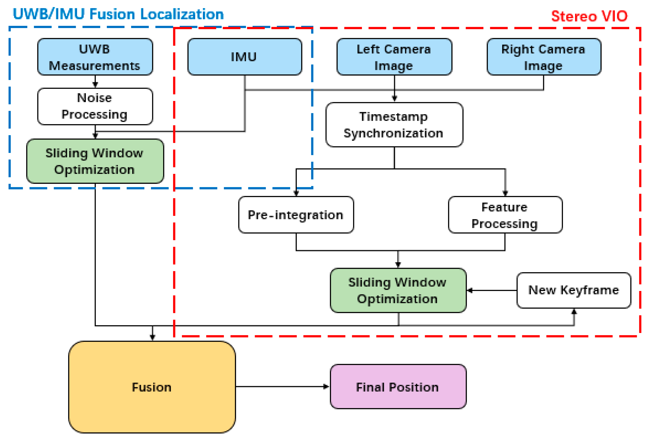
An indoor UWB and stereo VIO fusion localization method based on the EKF is proposed to enable long-term, accurate, and reliable real-time localization.
The remainder of this paper is organized as follows:
Section 3 presents the theoretical background of factor graphs and introduces a tightly coupled UWB/IMU fusion method based on factor graph optimization. Section 4 provides an overview of the EKF and details the proposed UWB–stereo VIO fusion localization method. Section 5 presents experimental validation and result analysis. Section 6 concludes the paper and outlines future research directions.

2. Related Work

2.1. Visual–Inertial Odometry

In GNSS-denied environments, VIO has become one of the most prominent solutions for motion estimation and mapping. By fusing the complementary information of visual and inertial sensors, VIO provides robust and accurate short-term localization [6]. Leutenegger et al. [9] introduced OKVIS, a keyframe-based VIO system that utilizes nonlinear optimization. Although it achieves high-quality localization and mapping, it lacks loop closure mechanisms, which results in the accumulation of drift over time. Similarly, Mourikis et al. [10] developed the Multi-State Constraint Kalman Filter (MSCKF), a filtering-based approach that reduces computational complexity by limiting state dimensionality, demonstrating good performance in large-scale real-world environments. Mur-Artal et al. [11] proposed a tightly coupled optimization-based VI-SLAM system that integrates loop closure to address the significant drift present in earlier VI systems. This system is capable of achieving unbiased pose estimation in looped trajectories and has been widely adopted in the research community. Shen et al. [12] from the Hong Kong University of Science and Technology developed the Visual–Inertial Navigation System-Mono (VINS-Mono), a robust monocular VIO system. It employs KLT optical flow tracking for front-end feature management and a sliding-window nonlinear optimization backend, while also integrating loop closure detection. This design offers excellent accuracy in diverse indoor and outdoor scenarios. Bloesch et al. [13] presented a VIO method based on an iterated extended Kalman filter (EKF), which minimizes photometric error from image patches. This approach achieves lightweight, real-time fusion of inertial and visual measurements and provides reliable localization performance even in the absence of loop closure. Campos et al. [14] introduced ORB-SLAM3, a feature-based SLAM framework that supports monocular, stereo, and inertial configurations. However, it is sensitive to environmental variations such as lighting changes. VINS-Mono [13] combines visual and inertial data using a sliding-window filter and requires careful initialization. Another notable contribution is OpenVINS [15], an open-source, real-time visual–inertial odometry system developed by Geneva et al. It supports monocular, stereo, and multi-camera configurations and is designed for easy integration and deployment in resource-constrained embedded systems. OpenVINS features a tightly coupled EKF backend and emphasizes repeatability, robustness, and portability, making it an attractive baseline system for real-time robotics applications.
Despite these significant advancements, current VIO systems still suffer from limitations such as accumulated drift, sensitivity to visual degradation (e.g., poor lighting, motion blur), and the lack of absolute positioning references.

2.2. UWB Positioning

UWB has become a prominent candidate for high-accuracy indoor localization due to its excellent time resolution, wide bandwidth, and robustness against multipath interference [8]. In indoor localization systems based on UWB, nodes are typically classified into two types: anchor nodes, which are fixed and known in position, and unknown nodes, which are mobile and require positioning. The unknown node’s location is calculated using its spatial relationship with multiple anchors [16].
Prorok et al. [17] proposed a Time Difference of Arrival (TDOA) measurement model for UWB, revealing the multimodal statistical distribution of UWB positioning error in space. Hanssens et al. [18] further characterized the geometric properties of UWB signal propagation, including arrival time delays, angles of arrival and departure, and the variances of these parameters. Common UWB localization techniques rely on Time of Arrival (TOA) [19], TDOA [20], and Two-Way Ranging (TWR) [21] measurement principles, with solution algorithms such as least squares, CHAN, and Taylor series methods [22]. In addition to these traditional approaches, intelligent optimization algorithms have gained popularity in recent years to improve estimation accuracy under non-ideal conditions [23]. For challenging environments with multipath and non-line-of-sight (NLOS) effects, various strategies have been proposed to mitigate signal distortion. For instance, B. Silva [24] introduced a high-accuracy localization system based on Symmetric Double-Sided Two-Way Ranging (SDS-TWR) combined with trilateration, which reduces errors introduced by timing offsets.
Deep learning has also been explored for direct signal processing. Reference [25] proposed a method to extract accurate ToA from raw Channel Impulse Response (CIR) data using a neural network, thereby enabling accurate positioning in multipath scenarios. Additionally, Ma et al. [26] proposed a hybrid solution that combines the C-Taylor weighting approach with an Adaptive Robust Kalman Filter (ARKF) to optimize the weight assignment of TOA measurements, effectively reducing the positioning error caused by NLOS conditions.
Overall, UWB provides a strong foundation for high-precision indoor localization. However, signal degradation in complex environments remains a challenge. To improve long-term accuracy and robustness, recent trends are increasingly exploring multi-sensor fusion frameworks, combining UWB with vision, IMU, or other modalities.

2.3. Multi-Sensor Fusion Strategies

Given the complementary strengths of VIO and UWB positioning, their integration has become a promising direction for achieving accurate and robust indoor localization. UWB, as an active positioning technique, provides absolute global position measurements, while VIO, as a passive method, ensures high-frequency relative pose estimation. Combining these modalities enables both global accuracy and local continuity.
In recent years, various fusion frameworks have been proposed. Reference [27] introduced a tightly coupled VIO-UWB fusion scheme, where VIO and UWB raw measurements are jointly optimized to estimate the robot’s pose. This approach achieves high accuracy but often requires complex, computation-intensive optimization. Reference [28] presented a loosely coupled monocular VIO system assisted by UWB, using an EKF [29] to integrate relative and absolute positioning information. EKF-based fusion is computationally efficient and suitable for real-time applications, though it may be sensitive to sensor noise models and linearization errors.
To address scalability and modularity, an optimization-based loosely coupled framework was proposed in [30], demonstrating that UWB data can effectively reduce drift in visual localization and enhance system robustness. In addition, graph-based optimization methods have gained significant attention. Notably, the Georgia Tech Smoothing and Mapping (GTSAM) [31] framework provides a flexible factor graph structure for fusing heterogeneous sensor inputs. GTSAM enables efficient batch or incremental optimization and is increasingly used in VIO-UWB fusion systems for its ability to model measurement constraints explicitly and maintain system consistency across time.

3. Tightly Coupled UWB/IMU Fusion Localization Based on Sliding-Window Factor Graph

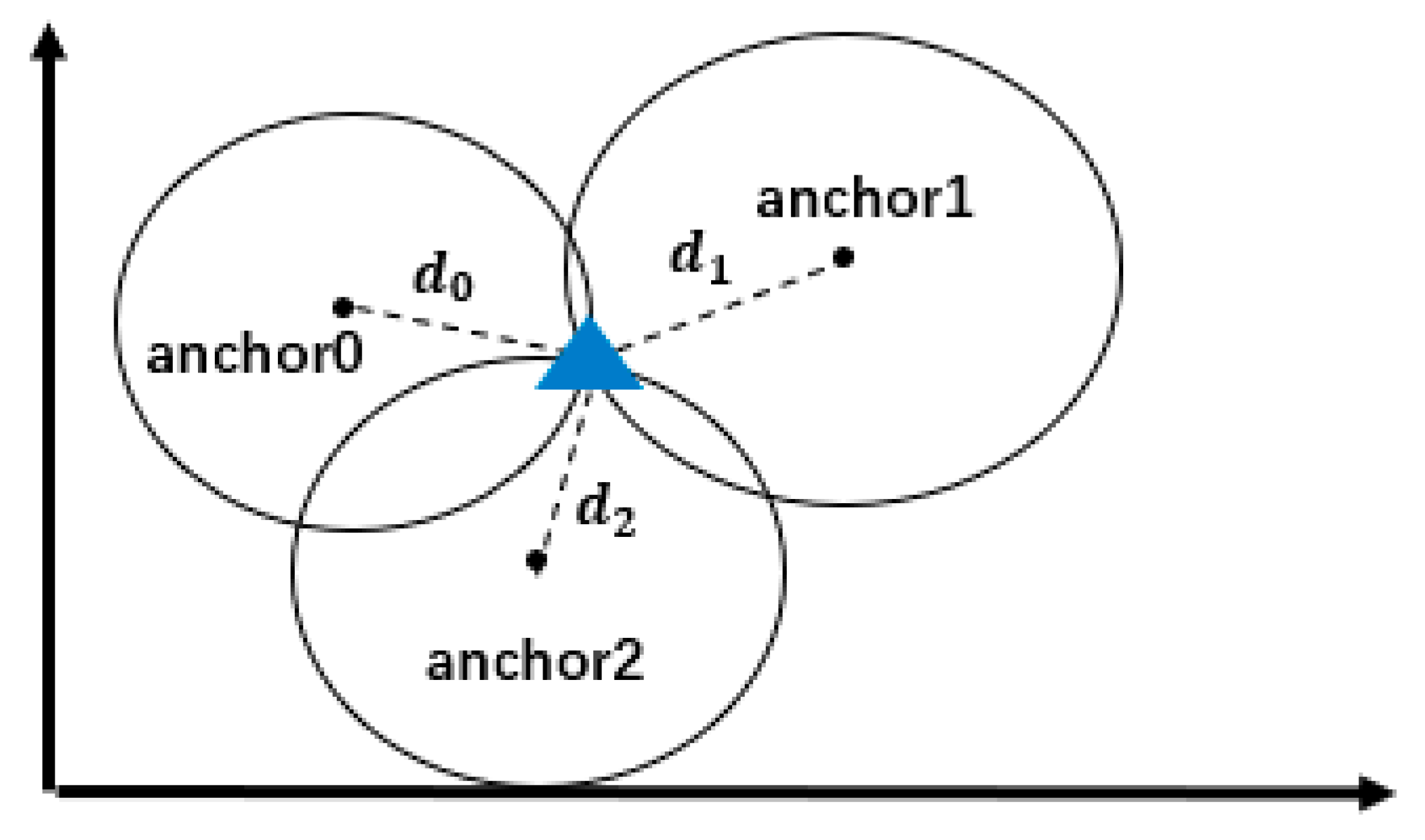
3.1. UWB Ranging Model

In fusion-based localization systems, UWB technology has been widely adopted for indoor positioning due to its high accuracy and strong resistance to multipath interference. Our system employs a TOA-based positioning method, which determines the signal propagation time by directly measuring the interval between when the UWB pulse is transmitted by the mobile station and when it is received by the reference station [32]. The distance is then calculated by multiplying the propagation time by the speed of light in free space. This distance is subsequently used to determine the position of the mobile station. Specifically, the UWB mobile station transmits a pulse signal at time t 1 and the reference station receives it at time t 2 . The propagation time is t 2 t 1 and the distance d i between the two stations is given by:
d i = c · t 2 t 1 + n i
Here, c denotes the speed of light, n i represents the measurement noise, and d i is the measured distance between the i -th reference station and the mobile station. In a two-dimensional localization scenario, let the unknown position of the UWB mobile station be denoted as ( x , y ) , and the known position of the i -th reference station be x i ,   y i . The corresponding TOA ranging equation can be expressed as:
d i = x x i 2 + y y i 2 + n i
As illustrated in Figure 1, by introducing multiple reference stations (at least three), the nonlinear equations can be jointly solved to accurately estimate the two-dimensional position of the UWB mobile station. This method achieves high ranging accuracy and stability, provided that strict time synchronization is maintained among all base stations. Compared with other positioning models such as TDOA and Angle of Arrival (AOA), the TOA-based method demonstrates superior absolute positioning performance in systems where hardware-level time synchronization is supported. It is particularly suitable for indoor navigation and mobile robotics applications that require high positioning accuracy.

3.2. Factor Graph-Based Fusion Localization

The core idea of factor graph-based navigation lies in constructing a global optimization model by establishing probabilistic constraints between system state variables and navigation observations. The optimal system state is then estimated under the maximum a posteriori (MAP) criterion. The system state X typically includes 3D position, velocity, attitude, and sensor biases. The observation data, denoted as Z , may originate from various sensors, including IMU, UWB, and cameras [33]. Within the probabilistic inference framework, the navigation and localization problem can be formulated as estimating the system state X that maximizes the posterior probability P ( X | Z ) given the observations Z . This leads to a MAP estimation problem:
X * = argmax x P X k : 1 Z k : 2 = argmax x P Z k : 2 X k : 1 P X k : 1 P Z k : 2
Here, k denotes the discrete time step. The term P ( Z k : 2 ) does not affect the estimation of the state variables. According to Bayes’ theorem, this expression is expanded as the product of a likelihood function and a prior distribution. Here, P ( Z k : 2 | X k : 1 ) denotes the likelihood of the observations given the state, reflecting the sensor measurement model. P ( X k : 1 ) represents the prior knowledge about the system states. In the factor graph model, state variables are represented as variable nodes, while sensor observations are formulated as factor nodes connected to the corresponding variables. This structure results in a sparse graphical representation.
X * = argmax x P Z k : 2 X k : 1 P X k : 1
Based on the first-order Markov assumption and the observation independence assumption.
P Z k : 2 X k : 1 = i = 2 k P z i x i
P X k : 1 = i = 2 k P x i x i 1 P x 1
Assuming that both process noise and measurement noise follow a Gaussian distribution, we obtain:
P x i x i 1 e x p 1 2 x i f x i 1 R i 2
P z i x i e x p 1 2 z i h x i Q i 2
f (   ) denotes the transition function that models the relationship between state variables x i 1 , and x i . h (   ) denotes the observation function relating the state variable x i to the measurement z i . R i denotes the measurement noise covariance matrix, and Q i denotes the process noise covariance matrix. Here, α i is an arbitrary vector. |   | R i 2 denotes the marginal distance with respect to the covariance matrix R i , and is computed as:
α i R i 2 = α i · R i · α i T
Therefore, the above equation can be reformulated as:
X * = argmax i = 2 k e x p 1 2 x i f x i 1 R i 2 × i = 2 k e x p 1 2 Z i h x i Q i 2
By simplifying the above expression, we obtain:
X * = argmax e x p 1 2 i = 1 k x i f x i 1 R i 2 + i = 1 k Z i h x i Q i 2
To achieve the maximum a posteriori probability, the cost function must be minimized; that is:
X * = argmin x i = 1 k x i f x i 1 R i 2 + i = 1 k Z i h x i Q i 2
Once the global cost function based on the MAP criterion is established, the state estimation problem in the navigation system can be transformed into a nonlinear least-squares optimization problem. The objective is to obtain the optimal state estimate by minimizing the cost function. Common methods for solving this optimization problem include the Gauss–Newton algorithm and the Levenberg–Marquardt algorithm. These algorithms iteratively approximate the local minimum of the objective function at each step.

3.3. UWB/IMU Fusion Localization

The sliding-window factor graph structure combining the UWB and IMU localization mechanisms is illustrated in Figure 2.
Let a i denote the system state at time i , which includes the object’s position along the x- and y-axes, i.e.,
a i = x i ,   y i
The IMU factor models the transition between the states a i 1 and a i . The UWB factor establishes the constraint between the state a i and the UWB range measurement. Based on the IMU measurement model, the corresponding cost function can be formulated as:
a i f I M U a i 1 R i 2 = a i a i 1 + s k × cos θ k s k × sin θ k R i 2
Here, θ k represents the yaw angle of the platform at time step k . f I M U ( ) is the IMU-based motion prediction function, and h U W B is the UWB measurement model. The cost function based on the UWB range measurement is given by:
z i h U W B a i Q i 2 = r j a i a n c j R i 2
The global cost function constructed from IMU and UWB factors can thus be expressed as:
X * = argmin a i = k k + w i n d o w a i f I M U a i 1 R i 2 + i = k k + w i n d o w z i h U W B a i Q i 2
In the global cost function, the sliding window is used to control the number of historical states involved in the optimization. When the number of states has not yet reached the predefined maximum window size, the actual length of the sliding window equals the current number of available states. Once the number of states reaches the threshold, the window maintains a fixed length by discarding the oldest state and incorporating the newest one in a first-in, first-out (FIFO) manner, enabling dynamic updates of the state sequence. Upon receiving new sensor data, the system constructs the current global cost function within the sliding window based on the included state nodes and their corresponding observations. This cost function incorporates residual terms from all sensor constraints and seeks the optimal solution in the state space. This optimization problem is typically solved using nonlinear optimization algorithms, such as the Gauss–Newton or Levenberg–Marquardt methods. By iteratively minimizing the sum of squared residuals, the optimal estimate of the state variables within the current window is obtained. The sliding window strategy significantly reduces computational complexity while preserving temporal continuity and observation redundancy, thereby enabling efficient and accurate real-time navigation. In this paper, the DogLeg algorithm is employed to solve the optimization problem.
The DogLeg algorithm is a widely used iterative method for solving nonlinear least-squares problems and is extensively applied in navigation and localization tasks such as factor graph optimization. Its core idea is to operate within a trust-region framework and combine the strengths of the Gauss–Newton and steepest descent methods by constructing a piecewise linear search path to efficiently determine the step direction. The DogLeg algorithm first computes the steepest descent step a i S D and the Gauss–Newton step a i G N . If a i G N lies within the trust region radius , it is directly accepted as the update step. If it exceeds the radius, a DogLeg path is constructed between a i S D and a i G N , and the point within the trust region along this path is selected as the update step a i d . At each iteration, the algorithm evaluates the step quality using a performance metric ρ .
ρ = F a i F a i + a i d L 0 L a i d
Here, F denotes the actual cost function, while L represents the second-order approximation of the model-predicted cost. If ρ is close to 1, the model prediction is considered accurate, and the trust-region radius is increased. If ρ is small or negative, it indicates that the current step is ineffective, and the trust-region radius should be reduced to improve convergence. This iterative process continues until the termination condition is met. The detailed steps are presented in Algorithm 1.
Algorithm 1 DogLeg Method
1: begin
2: intialize  k = 0   r = r 0
3: While  k < k max
4:   compute  g i = J a i 1 T F a i 1
5:   if  g i 2 t h 1  or  r i 1 t h 2 ( a i 1 2 + t h 2 )  or  F ( a i ) 2 t h 3
6:    break
7:   endif
8:    a i G N = J ( a i 1 ) T F ( a i 1 ) J ( a i 1 ) T J ( a i 1 )
9:    Δ a i S D = J ( a i 1 ) T F ( a i 1 )
10:   α = g i 2 2 J ( a i 1 ) g i 2 2
11:  if  Δ a i G N 2 r i 1
12:    Δ a i D L = Δ a i S D
13:  elseif  Δ a i S D 2 r i 1
14:    Δ a i D L = r i 1 Δ a i S D Δ a i S D 2
15:   else
16:     u = a i G N Δ a i S D
17:     a = u T u
18:     b = 2 Δ a i S D u
19:     c = Δ a i S D T Δ a i S D r i 1 2
20:     t a u = b + b 2 4 a c 2 a
21:     Δ a i D L = Δ a i S D + t a u u
22:   endif
23:  if  Δ a i D L 2 t h 2 a i 1 2 + t h 2
24:    break
25:   endif
26:   a i = a i 1 + Δ a i D L
27:   L 0 = 0.5 × f a i T f a i ;
28:   L Δ a i D L = f a i T f a i + Δ a D L T J a i T F a i + Δ a D L + 1 2 Δ a D L T J ( a i ) T J ( a i ) Δ a i D L ;
29:   ρ = F a i 1 f a i 1 T F a i F a i T L 0 L Δ a i D L
30:  if  ρ > 0.75
31:    r i = { m a x r i 1 , 3 × Δ a i D L 2 }
32:  elseif  ρ < 0.25
33:    r i = 0.5 r i 1
34:   endif
35:   k = k + 1
36: end

4. Stereo VIO/UWB Fusion Localization Algorithm

The two representative mainstream VIO algorithms are (1) the filter-based MSCKF, and (2) the optimization-based VINS. The MSCKF algorithm maintains the current IMU state and a limited number of past camera poses to construct constraints on feature observations without explicitly recovering the 3D positions of the features. As the MSCKF only retains a fixed number of camera states within a sliding window, its update and estimation process is strictly recursive. However, it cannot incorporate global observation information for consistent global pose optimization, which limits its ability to suppress long-term drift. In contrast, VINS introduces a sliding-window optimization framework that jointly incorporates IMU pre-integration and visual feature residuals into a nonlinear optimization problem, enabling batch optimization within the window and significantly improving localization accuracy. This method fully exploits the high-order correlations among all states within the window, making more effective use of observation data. It demonstrates robust and accurate trajectory reconstruction, especially in dynamic or low-texture environments.
Therefore, this paper adopts VINS for stereo VIO localization and integrates it with the aforementioned tightly coupled UWB/IMU fusion method based on a sliding-window factor graph. A filtering algorithm is then employed to fuse the localization results from both systems, in order to obtain the optimal position estimates of the mobile robot at each time step. The workflow of the stereo VIO/UWB fusion localization system is illustrated in Figure 3.

4.1. State Model Construction

The commonly used fusion method is the Kalman filter, which requires defining a state equation and a measurement equation based on the integrated positioning sources. It performs predictions using the state equation and updates using the observation equation to estimate the state vector. The standard Kalman filter assumes a linear state and observation models, whereas in practical scenarios, nonlinearities are often present. To address this issue, the EKF is employed for fusion-based state estimation. The nonlinear functions are linearized via first-order Taylor expansion, enabling the application of Kalman filtering to estimate the system’s position updates. In the UWB-VIO fusion system, the independent coordinate frame used by UWB is typically selected as the global reference frame for the entire system. The local VIO coordinate system is then transformed into this global frame to achieve spatial alignment of the sensor observations. The system state is modeled using the 2D position and velocity of the mobile platform. Assume that at time step k, the UWB and VIO measurements are approximately time-aligned, with the algorithm retrieving the most recent VIO data that precedes or closely matches the corresponding UWB timestamp. This allows both observations to jointly constrain the state estimation at this time step. The system state vector is defined as:
X k = x k y k v x , k v y , k T
Here, x k and y k denote the robot’s position in the 2D plane, while v x , k and v y , k represent the velocity components along the x- and y-axes, respectively. Assuming that the nominal state vector at time k is X ^ k and the associated error is δ X k , then the true state is given by X k = X ^ k + δ X k . The error-state model of the stereo VIO/UWB fusion system is defined as:
δ x k = δ x k 1 + δ v k 1 x t + t 2 2 a k 1 x δ y k = δ y k 1 + δ v k 1 y t + t 2 2 a k 1 y δ v k x = δ v k 1 x + a k 1 x t δ v k y = δ v k 1 y + a k 1 y t
Here, t denotes the sampling interval, and a k 1 x and a k 1 y represent the accelerations in the x and y directions at time k 1 . The nominal state X ^ k is initialized using the received VIO data, followed by an error-state update. By reorganizing Equation (19), the predicted error state and covariance at time k can be obtained, as shown in Equation (20).
δ X k | k 1 = F δ X k 1 + W k 1
where F = 1 0 t 0 0 1 0 t 0 0 1 0 0 0 0 1 is the system state transition matrix; W k 1 = t 2 2 a k 1 x t 2 2 a k 1 y a k 1 x t a k 1 y t represents the system noise vector.

4.2. Observation Model Construction

Upon obtaining the UWB/IMU localization data, a measurement equation can be constructed, where the difference between the UWB/IMU and VIO localization results is used as the observation vector Y k . The observation model for the stereo VIO/UWB fusion system is thus given by:
Y k = H δ X k + V k
where the observation vector is defined as Y k = x k U I x k V I O y k U I y k V I O , V k represents the observation noise, and the observation matrix is given by:
H = x k U I x k , i B k , i U I y k U I y k , i B k , i U I 0 0 x k V I O x k 1 V I O k , k 1 V I O y k V I O y k 1 V I O k , k 1 V I O 0 0
k , i U I = x k U I x k , i B 2 y k U I y k , i B 2
k , k 1 V I O = x k V I O x k 1 V I O 2 y k V I O y k 1 V I O 2
where x k U I , y k U I denote the UWB/IMU coordinates at time k ; x k , i B , y k , i B represent the coordinates of the i -th anchor at time k ; x k V I O , y k V I O and x k 1 V I O , y k 1 V I O are the stereo VIO coordinates at time steps k and k 1 .

4.3. Extended Kalman Filter

As shown in Equations (20) and (21), the proposed stereo VIO/UWB fusion system can be approximated as a linear system. Once the state and observation equations are established, state estimation can be performed using the standard Kalman filtering equations. The standard Kalman filter begins with a prediction step based on the state transition equation.
δ X k | k 1 = F δ X k 1 + W k 1 P k | k 1 = F P k 1 F T + Q k 1
The subsequent update step involves computing the Kalman gain K k , updating the error state δ X k | k , and revising the covariance matrix P k | k .
K k = P k | k 1 H T H P k | k 1 H T + R k 1 δ X k | k = δ X k | k 1 + K k Y k H δ X k | k 1 P k | k = I K k H P k | k 1
Here, R k denotes the observation noise covariance at time step k .

5. Experiments and Results Analysis

5.1. Experimental Platform Setup

5.1.1. Hardware Platform

The stereo localization platform employs the Intel RealSense D435i camera, which captures single-frame RGB images at a resolution of 640 × 480 pixels and a frame rate of 30 Hz. The UWB module is based on the Qorvo DW1000 chip, operating at a sampling frequency of 1 Hz. The IMU employs the ICM-42688 chip with a sampling frequency of 1000 Hz. As shown in Figure 4, all devices are integrated into a wearable testing that is vest worn by the test subject during data collection.

5.1.2. Software Platform

In this experiment, data acquisition and processing were integrated into a development board centered on the Orange Pi 5B for sensor fusion. All computing platforms ran on the Ubuntu 20.04 Linux operating system. The system was developed under the Robot Operating System (ROS) framework using Visual Studio Code v. 1.100.2 as the primary development tool. The ROS is an open-source meta-operating system designed specifically for robotics software development, featuring strong modularity and cross-platform compatibility. It provides hardware abstraction and device driver support for low-level robotic components, and integrates an efficient message-passing mechanism with a comprehensive toolchain and extensive open-source libraries for software retrieval, building, development, and execution. For multi-sensor fusion localization tasks, ROS offers unified data encapsulation and high-precision timestamp management for heterogeneous sensor inputs, enabling effective data alignment and temporal synchronization across different sensors. Based on this, the ROS built-in timestamping mechanism was employed to achieve time synchronization between monocular VIO and UWB measurements during fusion. In addition, the ROS integrates a powerful 3D visualization toolkit, RViz, which enables real-time 3D visualization of localization results by subscribing to trajectory topics published by the VIO module. This provides intuitive and effective support for system debugging and performance evaluation.

5.2. Experiment and Analysis

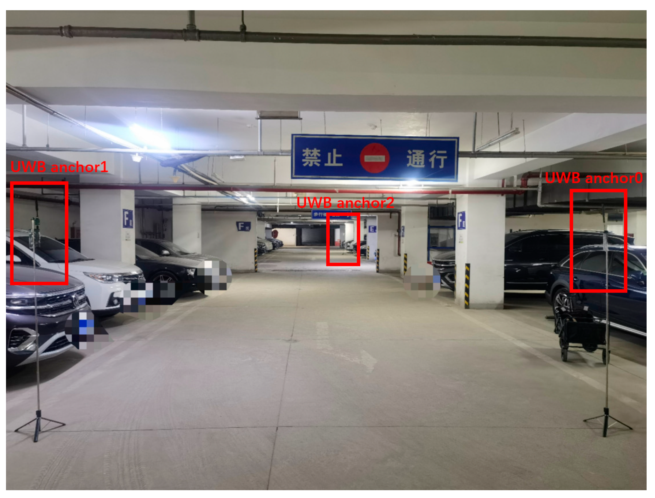
5.2.1. Experimental Scenario

To evaluate the positioning accuracy of the stereo VIO/UWB fusion system, the experiment was conducted in an underground parking garage, which is a common indoor localization environment, as shown in Figure 5. The environment is relatively open with good line-of-sight conditions, making it suitable for validating the system’s localization performance. As shown in Figure 6, the test subject walked along a rectangular path measuring 30 m in length and 4 m in width.
Four UWB modules were used in total, with three serving as fixed anchors and one mounted on the test subject as a mobile tag. The test subject moved at an approximately constant speed in a clockwise direction while collecting data.

5.2.2. Localization Accuracy Evaluation Criteria

Localization accuracy is typically evaluated using the root mean square error (RMSE), which quantifies the average deviation between the estimated trajectory and the ground truth. It reflects the overall error magnitude and provides a clear indication of the average trend in localization deviations. It is defined as follows:
R M S E = i = 1 n x i x ^ i 2 + y i y ^ i 2
Here, ( x i ,   y i ) denotes the ground-truth position at time step i , and x ^ i ,   y ^ i represents the corresponding estimated position.
C D F ( y ) = P e Y

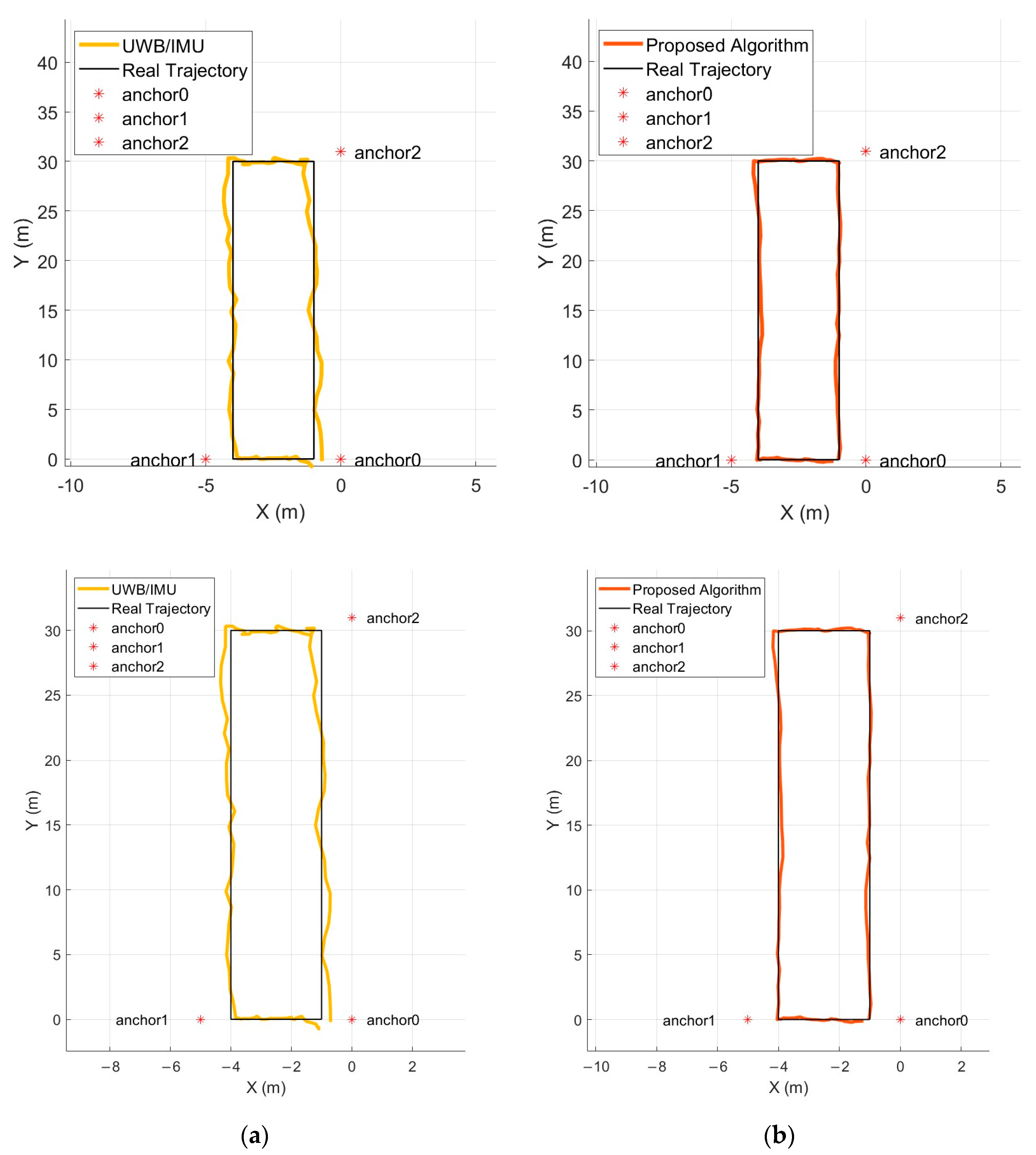
5.2.3. Results and Analysis

To evaluate the effectiveness of the proposed method, four comparative experiments were designed: (1) UWB-only localization, (2) UWB/IMU fusion localization, (3) stereo VIO-based localization, and (4) stereo VIO/UWB fusion localization.
The UWB data collected during the experiment were processed and compared against the ground-truth trajectory, as illustrated in Figure 7a. It can be observed that the UWB system provides higher localization accuracy when the user is close to the anchor nodes, but as the distance from the anchors increases, the trajectory begins to drift, which is particularly evident along the longer sides of the walking path. The maximum localization error in this scenario reaches 0.8446 m.
Using the stereo VIO model, estimated positions were obtained and compared with the actual walking trajectory, as shown in Figure 7b. It is evident that the system maintains high localization accuracy in the early phase of motion, but the trajectory gradually drifts over time due to cumulative error. The maximum localization error reaches 0.4997 m, especially when returning to the initial position.
The UWB/IMU fusion model was used for localization estimation and compared with the ground-truth trajectory, as shown in Figure 8a. Compared to the UWB-only system, the fusion model demonstrates higher localization accuracy, with reduced drift in regions far from the anchor nodes. The overall trajectory aligns more closely with the actual walking path. Although the factor graph-based UWB/IMU fusion model incorporates more historical states and observations, some drift still occurs in the latter part of the trajectory, resulting in increased error. The maximum localization error in this case is 0.3947 m.
The proposed model in this study was also used for localization estimation and was compared against the actual walking trajectory, as shown in Figure 8b. The EKF-based stereo VIO and UWB fusion system achieved superior localization accuracy, effectively addressing the drift commonly observed in VIO-only systems, while also mitigating the impact of UWB NLOS errors on the fusion system. As a result, the estimated trajectory is more consistent with the reference path. The maximum localization error of the fusion system is 0.2465 m.
Figure 9 presents the statistical localization errors for UWB, stereo VIO, UWB/IMU fusion models, and stereo VIO/UWB fusion models. As shown in Table 1, compared with the UWB-only method, the proposed algorithm improves localization accuracy by 67.6% and reduces the maximum error by approximately 67.9%. Compared with the stereo VIO model, the accuracy improves by 55.4%, and the maximum error decreases by about 60.4%. Compared with the UWB/IMU fusion model, it improves accuracy by 50.0% and reduces the maximum error by approximately 59.1%.

6. Conclusions

To address the limitations of stereo VIO—such as drift and significant localization errors in indoor environments—and the susceptibility of UWB to large errors under NLOS conditions, this study recognizes that single-sensor systems still struggle to meet the stability requirements of high-precision navigation. To overcome these challenges, this paper adopts the EKF to fuse UWB/IMU localization data with stereo VIO observations, and develops a UWB-VIO hybrid localization system based on the ROS platform for mobile robot applications. Comparative experiments demonstrate that the proposed method significantly improves localization accuracy and robustness in complex indoor environments. It effectively mitigates the drift problem in VIO and enhances the system’s resistance to NLOS interference.
Although the proposed filter-based fusion method provides good real-time performance and meets the continuous localization needs of indoor mobile robots, it still lags behind state-of-the-art graph-based optimization methods in terms of localization accuracy. Therefore, future work may explore the integration of filtering and optimization strategies to balance real-time performance with accuracy. In addition, the current method does not explicitly address the influence of environmental interference, including RF noise, signal multipath, or visual occlusions. These factors may degrade localization performance in dynamic or cluttered environments. In future research, we plan to incorporate interference-aware strategies in future research, such as robust outlier detection, adaptive covariance tuning, and sensor confidence weighting, to improve reliability.
Since the current system primarily performs localization in a two-dimensional plane, it does not fully account for dynamic variations in altitude. With the advancement of spatial operations, three-dimensional mobile platforms, such as unmanned aerial vehicles (UAVs), are expected to play a key role in indoor intelligent systems. Therefore, future research may extend to the development of 3D localization systems based on UAV platforms in order to meet the demands of higher-dimensional and more accurate localization applications. Moreover, although the current work mainly focuses on indoor scenarios due to the limitations of GNSS signals in such environments, we believe that the proposed method has the potential to be extended to outdoor or mixed environments. Future research may consider incorporating GNSS information to enhance localization robustness, especially in cases where UWB or visual features are limited.
Although the present work targets indoor positioning, we recognize that the core fusion strategies may be applicable in other domains facing similar challenges. For example, high-frequency surface wave radar (HFSWR) systems also require robust multi-source data integration under interference. Inspired by recent advances in high-resolution signal processing for HFSWR [34,35], future work may explore the cross-domain adaptation of our framework.

Author Contributions

Conceptualization, Z.D. and H.L.; methodology, H.L. and X.G.; software, H.L.; validation, H.L., P.L. and Z.D.; formal analysis, H.L.; investigation, H.L.; resources, H.L. and Z.D.; data curation, H.L.; writing—original draft preparation, H.L.; writing—review and editing, H.L.; visualization, H.L.; supervision, H.L. and Z.D.; project administration, H.L. All authors have read and agreed to the published version of the manuscript.

Funding

This research received no external funding.

Institutional Review Board Statement

Not applicable.

Informed Consent Statement

Not applicable.

Data Availability Statement

The original contributions presented in the study are included in the article, further inquiries can be directed to the corresponding authors.

Acknowledgments

We thank the Research Centre for Convergence of Wireless Network Communication and Navigation for their support for this research.

Conflicts of Interest

The authors declare no conflicts of interest.

References

  1. Yang, L.; Zhu, J.; Fu, Y.; Yu, Y. Integrity Monitoring for GNSS Precision Positioning. In Positioning and Navigation Using Machine Learning Methods; Springer: Berlin, Germany, 2024; pp. 59–75. [Google Scholar]
  2. Gan, X.; Yu, B.; Wang, X.; Yang, Y.; Jia, R.; Zhang, H.; Sheng, C.; Huang, L.; Wang, B. A New Array Pseudolites Technology for High Precision Indoor Positioning. IEEE Access 2019, 7, 153269–153277. [Google Scholar] [CrossRef]
  3. Xu, H.; Wang, L.; Zhang, Y.; Qiu, K.; Shen, S. Decentralized visual-inertial-UWB fusion for relative state estimation of Aerial Swarm. In Proceedings of the 2020 IEEE International Conference on Robotics and Automation (ICRA), Paris, France, 31 May 2020–31 August 2020; IEEE: New York, NY, USA, 2020; pp. 8776–8782. [Google Scholar]
  4. Cadena, C.; Carlone, L.; Carrillo, H.; Latif, Y.; Scaramuzza, D.; Neira, J.; Reid, I.; Leonard, J.J. Past, Present, and Future of Simultaneous Localization and Mapping: Toward the Robust-Perception Age. IEEE Trans. Robot. 2016, 32, 1309–1332. [Google Scholar] [CrossRef]
  5. Benini, A.; Adriano, M.; Sauro, L. An imu/uwb/vision-based extended kalman filter for mini-uav localization in indoor environment using 802.15.4a wireless sensor network. J. Intell. Robot. Syst. 2013, 70, 461–476. [Google Scholar] [CrossRef]
  6. Delmerico, J.; Davide, S. A benchmark comparison of monocular visual-inertial odometry algorithms for flying robots. In Proceedings of the 2018 IEEE International Conference on Robotics and Automation (ICRA), Brisbane, Australia, 21–25 May 2018; IEEE: New York, NY, USA, 2018. [Google Scholar]
  7. William, S.; Banerjee, S.; Hoover, A. Using a map of measurement noise to improve UWB indoor position tracking. IEEE Trans. Instrum. Meas. 2013, 62, 2228–2236. [Google Scholar]
  8. Shi, Q.; Cui, X.; Li, W.; Xia, Y.; Lu, M. Visual-UWB Navigation System for Unknown Environments. In Proceedings of the 31st International Technical Meeting of the Satellite Division of The Institute of Navigation (ION GNSS+ 2018), Miami, FL, USA, 24–28 September 2018; pp. 3111–3121. [Google Scholar]
  9. Leutenegger, S.; Lynen, S.; Bosse, M.; Siegwart, R.; Furgale, P. Keyframe-based visual–inertial odometry using nonlinear optimization. Int. J. Robot. Res. 2015, 34, 314–334. [Google Scholar] [CrossRef]
  10. Mourikis, A.I.; Stergios, I.R. A multi-state constraint Kalman filter for vision-aided inertial navigation. In Proceedings of the 2007 IEEE International Conference on Robotics and Automation, Rome, Italy, 10–14 April 2007; IEEE: New York, NY, USA, 2007. [Google Scholar]
  11. Mur-Artal, R.; Tardós, J.D. Visual-Inertial Monocular SLAM With Map Reuse. IEEE Robot. Autom. Lett. 2017, 2, 796–803. [Google Scholar] [CrossRef]
  12. Qin, T.; Li, P.; Shen, S. Vins-mono: A robust and versatile monocular visual-inertial state estimator. IEEE Trans. Robot. 2018, 34, 1004–1020. [Google Scholar] [CrossRef]
  13. Bloesch, M.; Omari, S.; Hutter, M.; Siegwart, R. Robust visual inertial odometry using a direct EKF-based approach. In Proceedings of the 2015 IEEE/RSJ International Conference on Intelligent Robots and Systems (IROS), Hamburg, Germany, 28 September 2015–2 October 2015; IEEE: New York, NY, USA, 2015. [Google Scholar]
  14. Campos, C.; Elvira, R.; Rodríguez, J.J.; Montiel, J.M.; Tardós, J.D. Orb-slam3: An accurate open-source library for visual, visual–inertial, and multimap slam. IEEE Trans. Robot. 2021, 37, 1874–1890. [Google Scholar] [CrossRef]
  15. Geneva, P.; Eckenhoff, K.; Lee, W.; Yang, Y.; Huang, G. OpenVINS: A Research Platform for Visual-Inertial Estimation. In Proceedings of the 2020 IEEE International Conference on Robotics and Automation (ICRA), Paris, France, 31 May 2020–31 August 2020; pp. 4666–4672. [Google Scholar] [CrossRef]
  16. Yu, T. Research on AGV Navigation and Positioning System Based on UWB, IMU and Vision Fusion. Master’s Thesis, Zhejiang University, Hangzhou, China, 2022. [Google Scholar]
  17. Prorok, A.; Martinoli, A. Accurate indoor localization with ultra-wideband using spatial models and collaboration. Int. J. Robot. Res. 2014, 33, 547–568. [Google Scholar] [CrossRef]
  18. Brecht, H.; David, P.; Emmeric, T.; Claude, O.; Davy, P.G.; Martine, L. An indoor variance-based localization technique utilizing the UWB estimation of geometrical propagation parameters. IEEE Trans. Antennas Propag. 2018, 66, 2522–2533. [Google Scholar]
  19. Taponecco, L.; D’Amico, A.A.; Mengali, U. Joint TOA and AOA estimation for UWB localization applications. IEEE Trans. Wirel. Commun. 2011, 10, 2207–2217. [Google Scholar] [CrossRef]
  20. Yun, C.; Zhou, T. UWB indoor positioning algorithm based on TDOA technology. In Proceedings of the 2019 10th International Conference on Information Technology in Medicine and Education (ITME), Qingdao, China, 23–25 August 2019; IEEE: New York, NY, USA, 2019. [Google Scholar]
  21. Sang, C.L.; Steinhagen, B.; Homburg, J.D.; Adams, M.; Hesse, M.; Rückert, U. Identification of NLOS and multi-path conditions in UWB localization using machine learning methods. Appl. Sci. 2020, 10, 3980. [Google Scholar] [CrossRef]
  22. Guo, Q.; Bu, L.; Song, X. Integrated navigation in indoor NLOS environment based on Kalman filter. In Proceedings of the 2021 5th International Conference on Electronic Information Technology and Computer Engineering, Xiamen, China, 22–24 October 2021; pp. 586–590. [Google Scholar]
  23. Li, T.; Deng, Z.; Wang, G.; Yan, J. Time difference of arrival location method based on improved snake optimization algorithm. In Proceedings of the 2022 IEEE 8th International Conference on Computer and Communications (ICCC), Chengdu, China, 9–12 December 2022; pp. 482–486. [Google Scholar]
  24. Silva, B.; Pang, Z.; Åkerberg, J.; Neander, J.; Hancke, G. Experimental study of UWB-based high precision localization for industrial applications. In Proceedings of the 2014 IEEE International Conference on Ultra-WideBand (ICUWB), Paris, France, 1–3 September 2014; pp. 280–285. [Google Scholar] [CrossRef]
  25. Niitsoo, A.; Edelhäußer, T.; Mutschler, C. Convolutional neural networks for position estimation in tdoa-based locating systems. In Proceedings of the Nternational Conference on Indoor Positioning and Indoor Navigation (IPIN), Nantes, France, 24–27 September 2018; pp. 1–8. [Google Scholar]
  26. Ma, W.; Fang, X.; Liang, L.; Du, J. Research on indoor positioning system algorithm based on UWB technology. Meas. Sens. 2024, 33, 101121. [Google Scholar] [CrossRef]
  27. Nguyen, T.H.; Nguyen, T.-M.; Xie, L. Range-focused fusion of camera-IMU-UWB for accurate and drift-reduced localization. IEEE Robot. Autom. Lett. 2021, 6, 1678–1685. [Google Scholar] [CrossRef]
  28. Nyqvist, H.E.; Skoglund, M.A.; Hendeby, G.; Gustafsson, F. Pose estimation using monocular vision and inertial sensors aided with ultra wide band. In Proceedings of the 2015 International Conference on Indoor Positioning and Indoor Navigation (IPIN), Banff, AB, Canada, 13–16 October 2015; IEEE: New York, NY, USA, 2015. [Google Scholar]
  29. Krishnaveni, B.V.; Reddy, K.S.; Reddy, P.R. Indoor positioning and tracking by coupling IMU and UWB with the extended Kalman filter. IETE J. Res. 2023, 69, 6757–6766. [Google Scholar] [CrossRef]
  30. Wang, C.; Zhang, H.; Nguyen, T.-M.; Xie, L. Ultra-wideband aided fast localization and mapping system. In Proceedings of the 2017 IEEE/RSJ International Conference on Intelligent Robots and Systems (IROS), Vancouver, BC, Canada, 24–28 September 2017; pp. 1602–1609. [Google Scholar] [CrossRef]
  31. Jurić, A.; Kendeš, F.; Marković, I.; Petrović, I. A Comparison of Graph Optimization Approaches for Pose Estimation in SLAM. In Proceedings of the 2021 44th International Convention on Information, Communication and Electronic Technology (MIPRO), Opatija, Croatia, 24–28 May 2021; pp. 1113–1118. [Google Scholar] [CrossRef]
  32. Alavi, B.; Pahlavan, K. Modeling of the TOA-based distance measurement error using UWB indoor radio measurements. IEEE Commun. Lett. 2006, 10, 275–277. [Google Scholar] [CrossRef]
  33. Lyu, P.; Wang, B.; Lai, J.; Bai, S.; Liu, M.; Yu, W. A factor graph optimization method for high-precision IMU-based navigation system. IEEE Trans. Instrum. Meas. 2023, 72, 9509712. [Google Scholar] [CrossRef]
  34. Golubović, D.; Erić, M.; Vukmirović, N.; Orlić, V. High-Resolution Sea Surface Target Detection Using Bi-Frequency High-Frequency Surface Wave Radar. Remote Sens. 2024, 16, 3476. [Google Scholar] [CrossRef]
  35. Golubović, D.; Erić, M.; Vukmirović, N. High-Resolution Azimuth Detection of Targets in HFSWRs Under Strong Interference. In Proceedings of the 2024 11th International Conference on Electrical, Electronic and Computing Engineering (IcETRAN), Nis, Serbia, 3–6 June 2024; pp. 1–6. [Google Scholar] [CrossRef]
Figure 1. Distance-based measurement method.
Applsci 15 06501 g001
Figure 2. UWB/IMU tightly coupled fusion localization based on sliding-window factor graphs.
Applsci 15 06501 g002
Figure 3. System architecture diagram.
Applsci 15 06501 g003
Figure 4. Integration demonstration.
Applsci 15 06501 g004
Figure 5. Underground garage environment.
Applsci 15 06501 g005
Figure 6. True trajectory of the underground garage.
Applsci 15 06501 g006
Figure 7. (a) The UWB-only localization results and the ground-truth trajectory; (b) the stereo VIO localization results and the ground-truth trajectory.
Applsci 15 06501 g007
Figure 8. (a) The UWB/IMU fusion model localization results and ground-truth trajectory; (b) the proposed model in this study’s localization results and ground-truth trajectory.
Applsci 15 06501 g008
Figure 9. (a) CDF of underground garage positioning results; (b) position error of underground garage with steps.
Applsci 15 06501 g009
Table 1. Comparison of localization error across algorithms.
Localization AlgorithmError MetricsError Magnitude (m)
UWBRMSE0.4212
MAX0.9297
VIORMSE0.3052
MAX0.7778
UWB/IMURMSE0.2722
MAX0.7515
Proposed AlgorithmRMSE0.1361
MAX0.3073
Disclaimer/Publisher’s Note: The statements, opinions and data contained in all publications are solely those of the individual author(s) and contributor(s) and not of MDPI and/or the editor(s). MDPI and/or the editor(s) disclaim responsibility for any injury to people or property resulting from any ideas, methods, instructions or products referred to in the content.

