
Triple-Stream Deep Feature Selection with Metaheuristic Optimization and Machine Learning for Multi-Stage Hypertensive Retinopathy Diagnosis


Abstract
1. Introduction
- A comprehensive literature analysis was conducted to examine existing AI-based studies in the diagnosis of eye diseases.
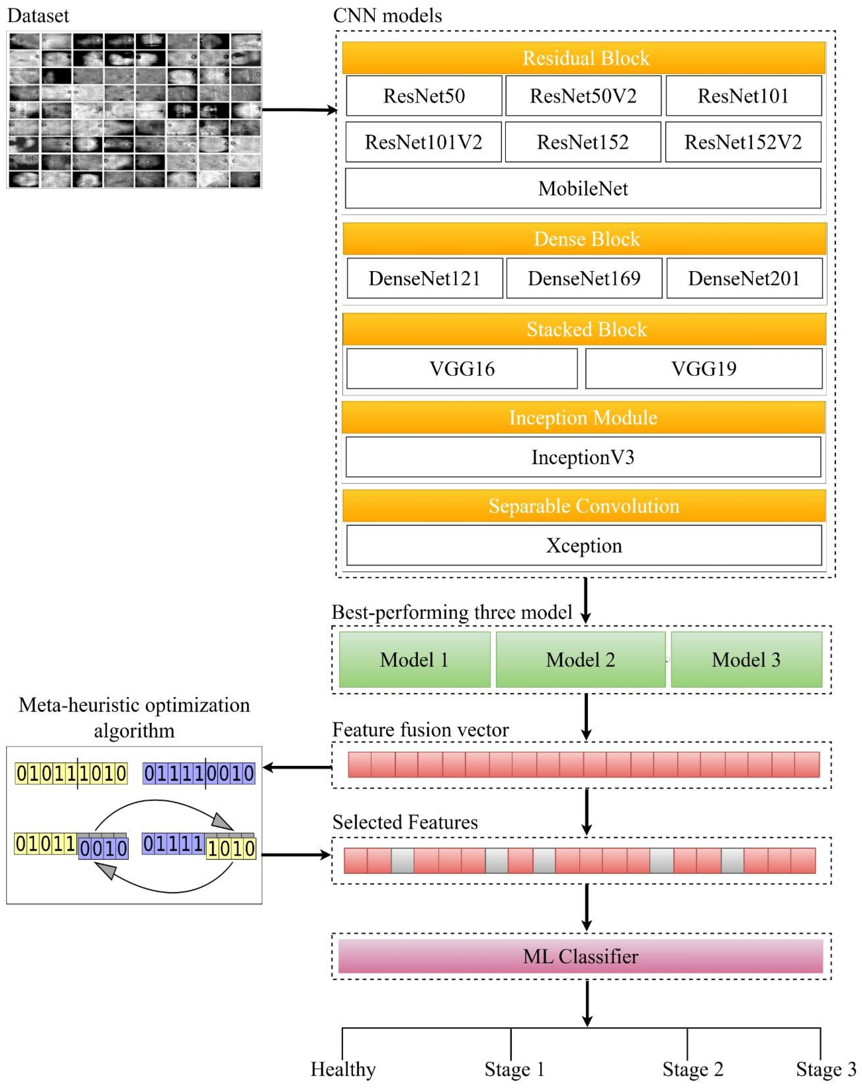
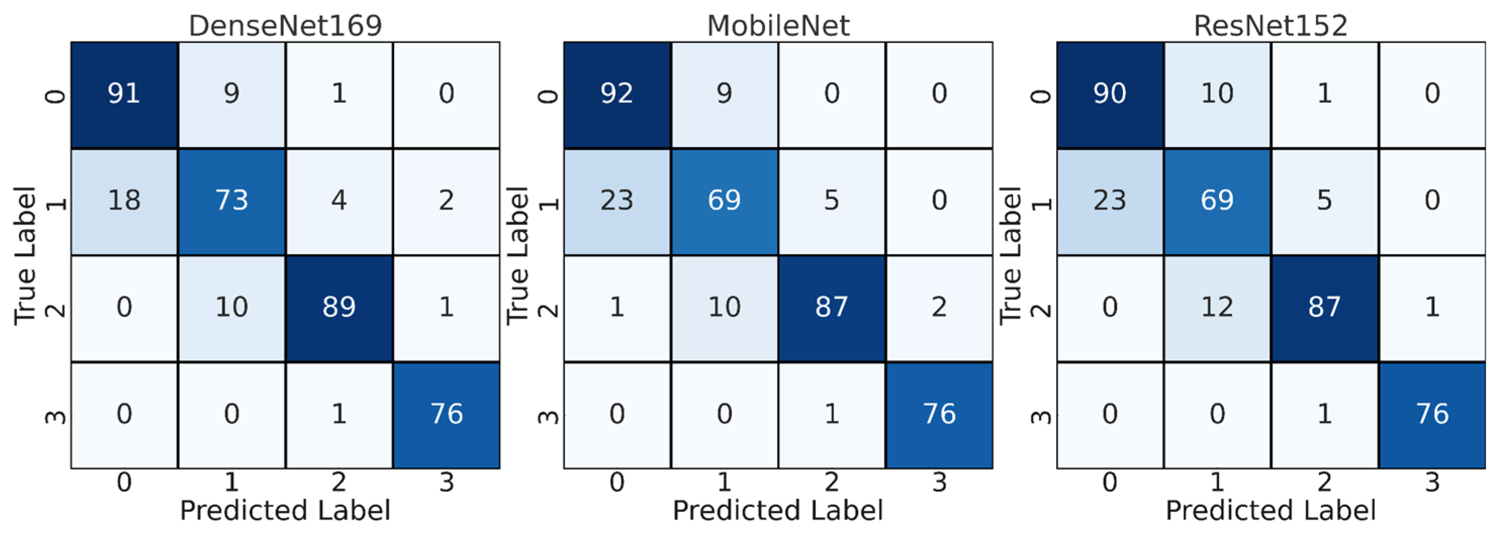
- Fourteen different CNN models commonly used in the literature were trained on a custom HR dataset and the three best-performing models were determined.
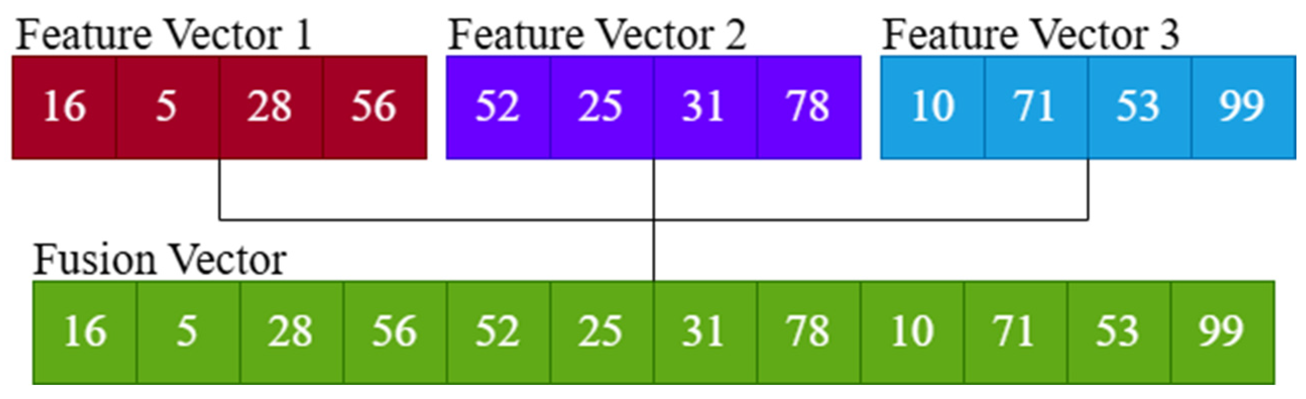
- Deep features extracted from the top three CNN models were combined to create a more robust feature set.
- The combined features were classified by ML algorithms (SVM, RF and XGBoost).
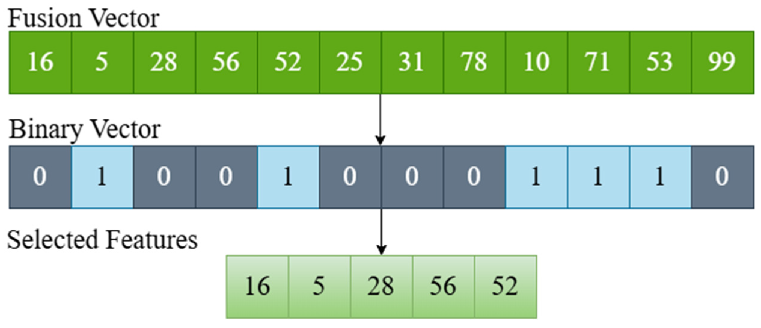
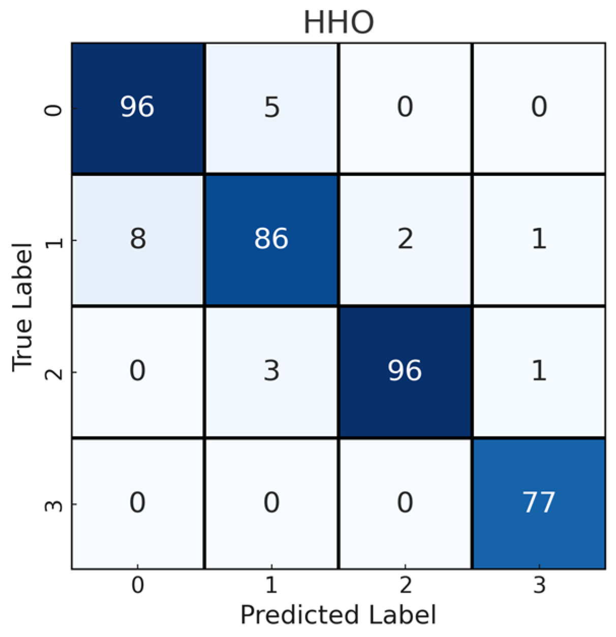
- GA, ABC, PSO and HHO methods were used in the feature selection process.
- The classification performance of the model was analyzed using extensive experiments and different evaluation metrics.
2. Materials and Methods
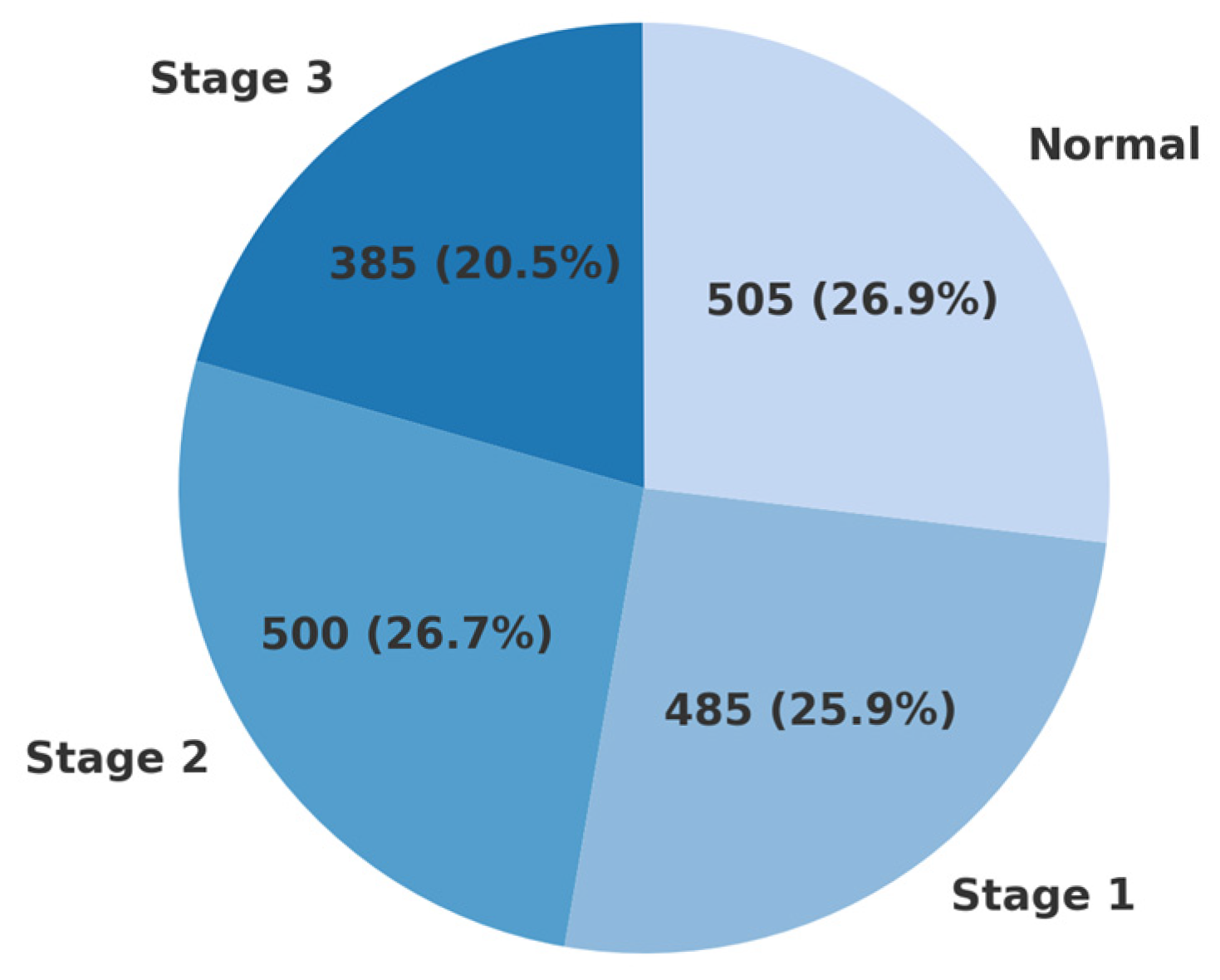
2.1. Dataset
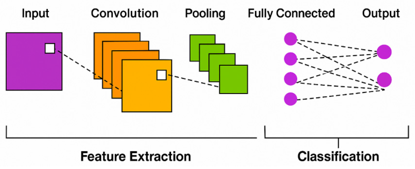
2.2. CNN
2.3. Transfer Learning
2.4. ML Algorithms
2.4.1. SVM
2.4.2. RF
2.4.3. XGBoost
2.5. CNN-Based Feature Extraction and Fusion
2.6. Feature Selection with Metaheuristic Optimization Algorithms
3. Experimental Setup
3.1. Experiment Setting
3.2. Evaluation Metrics
4. Results
4.1. CNN Results
4.2. Feature Fusion Results
4.3. Feature Selection Results
5. Discussion
6. Limitations and Future Work
7. Conclusions
Author Contributions
Funding
Institutional Review Board Statement
Informed Consent Statement
Data Availability Statement
Conflicts of Interest
References
- Shen, C.J.; Kry, S.F.; Buchsbaum, J.C.; Milano, M.T.; Inskip, P.D.; Ulin, K.; Francis, J.H.; Wilson, M.W.; Whelan, K.F.; Mayo, C.S.; et al. Retinopathy, optic neuropathy, and cataract in childhood cancer survivors treated with radiation therapy: A PENTEC comprehensive review. Int. J. Radiat. Oncol. Biol. Phys. 2024, 119, 431–445. [Google Scholar] [CrossRef] [PubMed]
- Ba, M.; Li, Z. The impact of lifestyle factors on myopia development: Insights and recommendations. AJO Int. 2024, 1, 100010. [Google Scholar] [CrossRef]
- Uyar, K.; Yurdakul, M.; Taşdemir, Ş. Abc-based weighted voting deep ensemble learning model for multiple eye disease detection. Biomed. Signal Process. Control 2024, 96, 106617. [Google Scholar] [CrossRef]
- Shin, H.J.; Costello, F. Imaging the optic nerve with optical coherence tomography. Eye 2024, 38, 2365–2379. [Google Scholar] [CrossRef] [PubMed]
- Li, Y.; Daho, M.E.H.; Conze, P.-H.; Zeghlache, R.; Le Boité, H.; Tadayoni, R.; Cochener, B.; Lamard, M.; Quellec, G. A review of deep learning-based information fusion techniques for multimodal medical image classification. Comput. Biol. Med. 2024, 177, 108635. [Google Scholar] [CrossRef]
- Shoukat, A.; Akbar, S.; Hassan, S.A.; Iqbal, S.; Mehmood, A.; Ilyas, Q.M. Automatic diagnosis of glaucoma from retinal images using deep learning approach. Diagnostics 2023, 13, 1738. [Google Scholar] [CrossRef]
- Patel, R.K.; Chouhan, S.S.; Lamkuche, H.S.; Pranjal, P. Glaucoma diagnosis from fundus images using modified Gauss-Kuzmin-distribution-based Gabor features in 2D-FAWT. Comput. Electr. Eng. 2024, 119, 109538. [Google Scholar] [CrossRef]
- Sharma, S.K.; Muduli, D.; Priyadarshini, R.; Kumar, R.R.; Kumar, A.; Pradhan, J. An evolutionary supply chain management service model based on deep learning features for automated glaucoma detection using fundus images. Eng. Appl. Artif. Intell. 2024, 128, 107449. [Google Scholar] [CrossRef]
- Geetha, A.; Sobia, M.C.; Santhi, D.; Ahilan, A. DEEP GD: Deep learning based snapshot ensemble CNN with EfficientNet for glaucoma detection. Biomed. Signal Process. Control 2025, 100, 106989. [Google Scholar] [CrossRef]
- Muthukannan, P. Optimized convolution neural network based multiple eye disease detection. Comput. Biol. Med. 2022, 146, 105648. [Google Scholar]
- Kihara, Y.; Shen, M.; Shi, Y.; Jiang, X.; Wang, L.; Laiginhas, R.; Lyu, C.; Yang, J.; Liu, J.; Morin, R.; et al. Detection of nonexudative macular neovascularization on structural OCT images using vision transformers. Ophthalmol. Sci. 2022, 2, 100197. [Google Scholar] [CrossRef] [PubMed]
- Gu, Y.; Fang, L.; Mou, L.; Ma, S.; Yan, Q.; Zhang, J.; Liu, F.; Liu, J.; Zhao, Y. A ranking-based multi-scale feature calibration network for nuclear cataract grading in AS-OCT images. Biomed. Signal Process. Control 2024, 90, 105836. [Google Scholar] [CrossRef]
- Liu, Y.; Yao, D.; Ma, Y.; Wang, H.; Wang, J.; Bai, X.; Zeng, G.; Liu, Y. STMF-DRNet: A multi-branch fine-grained classification model for diabetic retinopathy using Swin-TransformerV2. Biomed. Signal Process. Control 2025, 103, 107352. [Google Scholar] [CrossRef]
- Kulyabin, M.; Zhdanov, A.; Nikiforova, A.; Stepichev, A.; Kuznetsova, A.; Ronkin, M.; Borisov, V.; Bogachev, A.; Korotkich, S.; Constable, P.A.; et al. Octdl: Optical coherence tomography dataset for image-based deep learning methods. Sci. Data 2024, 11, 365. [Google Scholar] [CrossRef] [PubMed]
- Irshad, S.; Akram, M.U. Classification of retinal vessels into arteries and veins for detection of hypertensive retinopathy. In Proceedings of the 2014 Cairo International Biomedical Engineering Conference (CIBEC), Cairo, Egypt, 11–13 December 2014; IEEE: New York, NY, USA, 2015. [Google Scholar]
- Abbas, Q.; Qureshi, I.; Ibrahim, M.E. An automatic detection and classification system of five stages for hypertensive retinopathy using semantic and instance segmentation in DenseNet architecture. Sensors 2021, 21, 6936. [Google Scholar] [CrossRef]
- Suman, S.; Tiwari, A.K.; Sachan, S.; Singh, K.; Meena, S.; Kumar, S. Severity grading of hypertensive retinopathy using hybrid deep learning architecture. Comput. Methods Programs Biomed. 2025, 261, 108585. [Google Scholar] [CrossRef]
- Khan, A.; Sohail, A.; Zahoora, U.; Qureshi, A.S. A survey of the recent architectures of deep convolutional neural networks. Artif. Intell. Rev. 2020, 53, 5455–5516. [Google Scholar] [CrossRef]
- Pacal, I.; Ozdemir, B.; Zeynalov, J.; Gasimov, H.; Pacal, N. A novel CNN-ViT-based deep learning model for early skin cancer diagnosis. Biomed. Signal Process. Control 2025, 104, 107627. [Google Scholar] [CrossRef]
- Pacal, I. Investigating deep learning approaches for cervical cancer diagnosis: A focus on modern image-based models. Eur. J. Gynaecol. Oncol. 2025, 46, 125–141. [Google Scholar]
- Liang, J.; Liang, R.; Wang, D. A novel lightweight model for tea disease classification based on feature reuse and channel focus attention mechanism. Eng. Sci. Technol. Int. J. 2025, 61, 101940. [Google Scholar] [CrossRef]
- Zhong, J.; Tian, W.; Xie, Y.; Liu, Z.; Ou, J.; Tian, T.; Zhang, L. PMFSNet: Polarized multi-scale feature self-attention network for lightweight medical image segmentation. Comput. Methods Programs Biomed. 2025, 261, 108611. [Google Scholar] [CrossRef] [PubMed]
- Gao, Y.; Zhang, J.; Wei, S.; Li, Z. PFormer: An efficient CNN-Transformer hybrid network with content-driven P-attention for 3D medical image segmentation. Biomed. Signal Process. Control 2025, 101, 107154. [Google Scholar] [CrossRef]
- Shoaib, M.R.; Emara, H.M.; Mubarak, A.S.; Omer, O.A.; El-Samie, F.E.A.; Esmaiel, H. Revolutionizing diabetic retinopathy diagnosis through advanced deep learning techniques: Harnessing the power of GAN model with transfer learning and the DiaGAN-CNN model. Biomed. Signal Process. Control 2025, 99, 106790. [Google Scholar] [CrossRef]
- Muthusamy, D.; Palani, P. Deep neural network model for diagnosing diabetic retinopathy detection: An efficient mechanism for diabetic management. Biomed. Signal Process. Control 2025, 100, 107035. [Google Scholar] [CrossRef]
- Mewada, H.; Pires, I.M.; Engineer, P.; Patel, A.V. Fabric surface defect classification and systematic analysis using a cuckoo search optimized deep residual network. Eng. Sci. Technol. Int. J. 2024, 53, 101681. [Google Scholar] [CrossRef]
- He, K.; Zhang, X.; Ren, S.; Sun, J. Deep residual learning for image recognition. In Proceedings of the IEEE Conference on Computer Vision and Pattern Recognition, Las Vegas, NV, USA, 26 June–1 July 2016. [Google Scholar]
- Huang, G.; Liu, Z.; van der Maaten, L.; Weinberger, K.Q. Densely connected convolutional networks. In Proceedings of the IEEE Conference on Computer Vision and Pattern Recognition, Honolulu, HI, USA, 21–26 July 2017. [Google Scholar]
- Simonyan, K.; Zisserman, A. Very deep convolutional networks for large-scale image recognition. arXiv 2014, arXiv:1409.1556. [Google Scholar]
- Chollet, F. Xception: Deep learning with depthwise separable convolutions. In Proceedings of the IEEE Conference on Computer Vision and Pattern Recognition, Honolulu, HI, USA, 21–26 July 2017. [Google Scholar]
- Szegedy, C.; Liu, W.; Jia, Y.; Sermanet, P.; Reed, S.; Anguelov, D.; Erhan, D.; Vanhoucke, V.; Rabinovich, A. Going deeper with convolutions. In Proceedings of the IEEE Conference on Computer Vision and Pattern Recognition, Boston, MA, USA, 7–12 June 2015. [Google Scholar]
- Howard, A.G.; Zhu, M.; Chen, B.; Kalenichenko, D.; Wang, W.; Weyand, T.; Andreetto, M.; Adam, H. Mobilenets: Efficient convolutional neural networks for mobile vision applications. arXiv 2017, arXiv:1704.04861. [Google Scholar]
- Lu, J.; Behbood, V.; Hao, P.; Zuo, H.; Xue, S.; Zhang, G. Transfer learning using computational intelligence: A survey. Knowl.-Based Syst. 2015, 80, 14–23. [Google Scholar] [CrossRef]
- Alzubi, J.; Nayyar, A.; Kumar, A. Machine learning from theory to algorithms: An overview. J. Phys. Conf. Ser. 2018, 1142, 012012. [Google Scholar] [CrossRef]
- Cortes, C.; Vapnik, V. Support-Vector networks. Mach. Learn. 1995, 20, 273–297. [Google Scholar] [CrossRef]
- Breiman, L. Random forests. Mach. Learn. 2001, 45, 5–32. [Google Scholar] [CrossRef]
- Chen, T.; Guestrin, C. Xgboost: A scalable tree boosting system. In Proceedings of the 22nd ACM Sigkdd International Conference on Knowledge Discovery and Data Mining, San Francisco, CA, USA, 13–17 August 2016. [Google Scholar]
- Yurdakul, M.; Uyar, K.; Taşdemir, Ş. Enhanced ore classification through optimized CNN ensembles and feature fusion. Iran J. Comput. Sci. 2025, 8, 491–509. [Google Scholar] [CrossRef]


| Author(s) and Reference | Year | Methodology | Imaging Technique | Disease | Results | Merits | Limitations |
|---|---|---|---|---|---|---|---|
| Irshad et al. [15] | 2014 | SVM-based classification using intensity features | Fundus | HR | Accuracy: 81.3% | Simple and interpretable method | Small dataset, low accuracy |
| Abbas et al. [16] | 2021 | DenseNet-based semantic segmentation | Fundus | HR | Accuracy: 92.6% Sensitivity: 90.5% Specificity: 91.5% | High classification performance across stages | Limited scalability to other datasets |
| Muthukannan [10] | 2022 | CNN-based feature extraction and SVM | Fundus | AMD, DR, Cataract, Glaucoma, Normal | Accuracy: 98.30% Recall: 95.27% Specificity: 98.28% F1-Score: 93.3% | Very high accuracy and recall | Dataset-specific optimization; may overfit |
| Kihara et al. [11] | 2022 | ViT-based segmentation model using encoder–decoder architecture | OCT | neMNV | Sensitivity: 82% Specificity: 90% PPV: 79% NPV: 91% AUC: 0.91 | Strong generalization; human-level performance | Focused only on neMNV in AMD |
| Shoukat et al. [6] | 2023 | ResNet-50 architecture with transfer learning and data augmentation | Fundus | Glaucoma | Accuracy: 98.48% Sensitivity: 99.30% Specificity: 96.52% AUC: 97% F1-Score: 98% | Excellent performance with transfer learning | Limited generalizability; single disease |
| Patel et al. [7] | 2024 | FAWT and GKDG based feature extraction and LS-SVM. | Fundus | Glaucoma | Accuracy: 95.84% Specificity: 97.17% Sensitivity: 94.55% | Effective feature engineering approach | Complex preprocessing pipeline |
| Gu et al. [12] | 2024 | A ranking-based multi-scale feature calibration network | OCT | Cataract | Accuracy: 88.86% Sensitivity: 89.08% Precision: 90.15% F1-Score: 89.49% | Fine-grained severity classification | Narrow disease focus |
| Sharma et al. [8] | 2024 | Customized CNN, PCA + LDA for dimensionality reduction, ELM optimized with MOD-PSO | Fundus | Glaucoma | G1020 Dataset: Accuracy: 97.80% Sensitivity: 94.92% Specificity: 98.44% ORIGA Dataset: Accuracy: 98.46% Sensitivity: 97.01% Specificity: 98.96% | Optimized feature selection boosted results | Relatively complex architecture |
| Kulyabin et al. [14] | 2024 | ResNet50 and VGG16 | OCT | AMD, DME, ERM, RAO, RVO, VID, Normal | ResNet50: Accuracy: 84.6% Precision: 89.8% Recall: 84.6% F1-Score: 86.6% VGG16: Accuracy: 85.9% Precision: 88.8% Recall: 85.9% F1-Score: 86.9% | Benchmarking with multiple models and diseases | Accuracy moderate compared to others |
| Geetha et al. [9] | 2025 | EfficientNetB4, Snapshot Ensemble, Aquila Optimization and V-Net | Fundus | Glaucoma | Accuracy: 99.35% Precision: 99.04% Specificity: 99.19% Recall: 98.89% F1-Score: 98.97% | Extremely high accuracy and precision | High computational requirements |
| Liu et al. [13] | 2025 | STMF-DRNet | Fundus | DR | Accuracy:77% Sensitivity: 77% Specificity: 94.2% F1-Score: 77% Kappa: 87.7% | Advanced attention mechanisms for DR | Moderate accuracy; DR-specific only |
| Suman et al. [17] | 2025 | Hybrid DL model (ResNet-50 and ViT) | Fundus | HR | Accuracy: 96.88% Sensitivity: 94.35% Specificity: 97.66% F1-Score: 94.42% | Best-in-class hybrid performance | Resource-intensive and complex |
| Category | Identification |
|---|---|
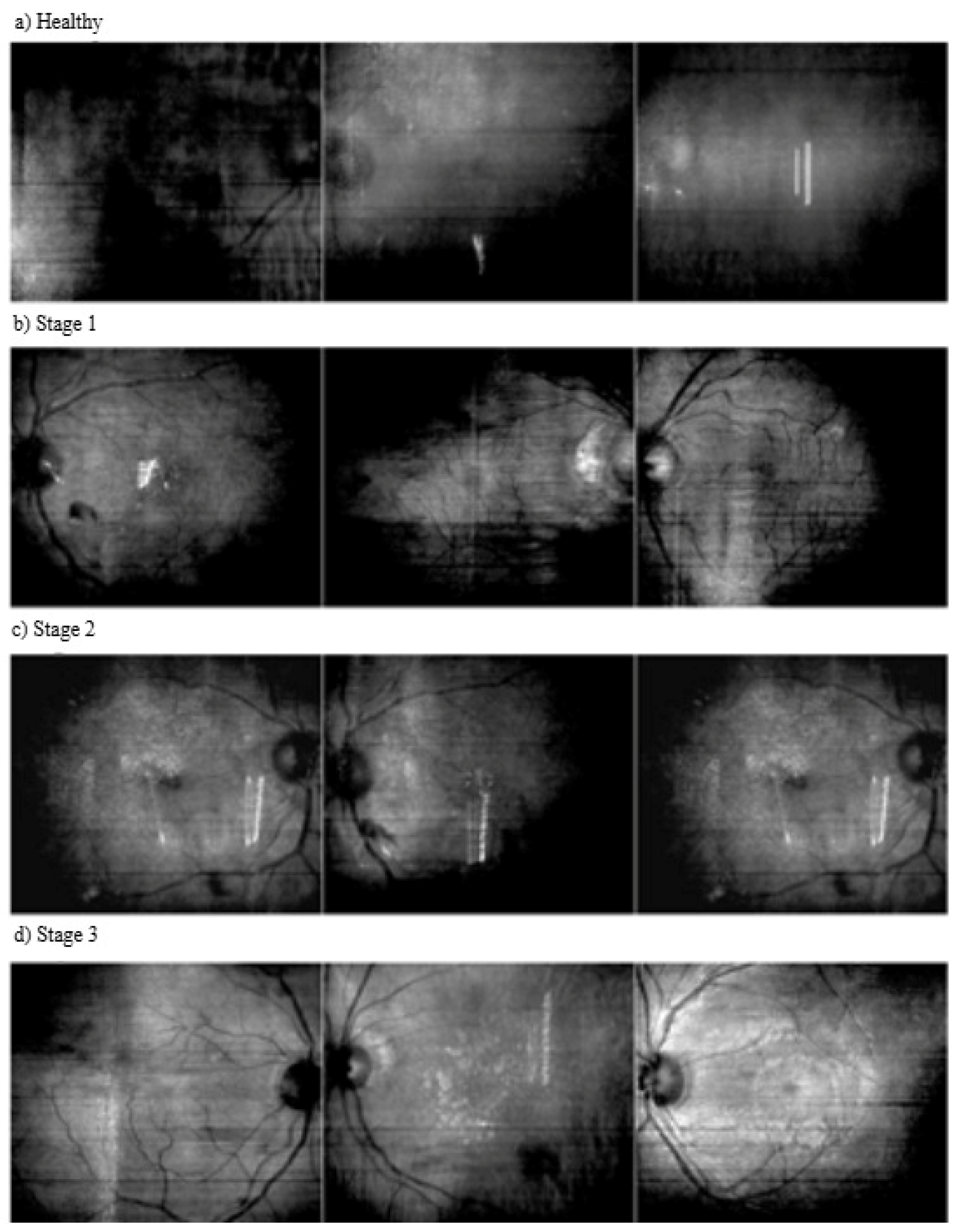
| Normal | No hypertension-related changes or abnormalities in the retina. |
| Stage 1 | A condition with mild arterial narrowing and thickening of the vessel walls. |
| Stage 2 | A condition with more pronounced vasoconstriction, arteriovenous crossing and atherosclerosis. |
| Stage 3 | A condition involving serious vascular disorders with hemorrhages, exudates and cotton wool-like spots in the retina. |
| Algorithm | Working Principle | Pseudocode | Merits | Limitations |
|---|---|---|---|---|
| GA | Based on the principles of natural selection and genetic evolution. Solutions are improved from generation to generation using genetic operators (selection, crossover, mutation). New solutions are generated by selecting the best individuals and the process continues until the optimum solution is reached. | Initialize population X randomly for t = 1…T: evaluate fitness f(X) P ← select parents from X C ← crossover P with rate α mutate C with rate pm X ← form new generation from X and C return best individual | Robust global search in complex search spaces | Requires parameter configuration; convergence speed is moderate |
| ABC | Mimics the behavior of honeybees searching for food sources. Three types of bees (worker, observer and explorer) try to find the best solutions. While developing good solutions, they also keep discovering new ones. | Initialize nectar sources {xi} randomly repeat: // Employed bees for each xi: x’i ← xi + φ·(xi − xk) if f(xi’) > f(xi): xi ← x’i // Onlooker bees compute pi = f(xi)/Σf(xj) select sources by pi and apply employed-bee step // Scout bees if trial[i] > limit: xi ← LB + rand·(UB − LB) until stopping criterion return best xi | Good exploration diversity; simple implementation | Convergence speed moderate; exploitation could improve |
| PSO | Emulates the collective movements of flocks of birds and schools of fish. Each particle (solution candidate) moves in line with its own best position and the swarm’s best position. Velocity updates are based on cognitive (personal best) and social (swarm best) components. | Initialize each particle i: position xi, velocity vi, personal best pi = xi g ← best of all pi for t = 1…T: for each particle i: vi ← w·vi + c1·rand·(pi − xi) + c2·rand·(g − xi) xi ← xi + vi if f(xi) < f(pi): pi ← xi if f(pi) < f(g): g ← pi return g | Fast convergence; few parameters to tune | Risk of local optima; may need restarts |
| HHO | Inspired by the hunting strategies of Harris’s hawks. It works in a balanced way between exploration (searching for prey) and exploitation (capturing prey), both seeking new solutions and improving existing ones. | Initialize hawks xi randomly within [LB, UB] for t = 1…T: E0 ← random in (−1,1) E ← 2·E0·(1 − t/T) Xbest ← hawk with best f if |E| ≥ 1: // exploration update Xi by random exploration formulas else: // exploitation J ← 2·(1 − rand) if |E| ≥ 0.5: Xi ← Xbest − E·|J·Xbest − Xi| else: Δ ← Xbest − Xi Xi ← Δ − E·|Δ| // optional: apply Lévy flight for further diversification return Xbest | Balanced exploration–exploitation; strong adaptability | Computationally more intensive; moderate implementation complexity |
| Configuration | Parameter |
|---|---|
| Operating System | Windows 11, 64 Bit |
| Programming Language | Python version 3.11.4 |
| Fameworks | Tensorflow 2.14.0, Keras version 2.11.4, Matplotlib 3.7.1 |
| GPU | 2 x Nvidia RTX 3090 24 GB |
| CPU | Intel(R) Core(TM) i9-10920X CPU @ 3.50 GHz |
| RAM | 128 GB |
| CUDA | v12.7 |
| Batch Size | Epoch | Learning Rate | Optimizer | Weights_Decay_Rate |
|---|---|---|---|---|
| 64 | 100 | 0.0003 | Adam | 0.9 |
| Metric | Equation | Description |
|---|---|---|
| Accuracy | Refers to the proportion of the model’s total predictions that are correct. | |
| Precision | Refers to the proportion of positive predicted samples that are actually positive. | |
| Recall | Measures how many true positive samples are correctly predicted. | |
| F1-Score | Provides the balance between precision and sensitivity. | |
| Cohen’s kappa score | Assesses how well the model performs compared to random guessing and is calculated based on observed accuracy (p0) and expected accuracy (pe). |
| Model | Accuracy | Precision | Recall | F1-Score | Kappa |
|---|---|---|---|---|---|
| DenseNet121 | 82.93 | 82.68 | 82.93 | 82.67 | 0.7717 |
| DenseNet169 | 87.73 | 87.75 | 87.73 | 87.67 | 0.8359 |
| DenseNet201 | 85.07 | 84.91 | 85.07 | 84.83 | 0.8002 |
| InceptionV3 | 82.13 | 81.67 | 82.13 | 81.60 | 0.7616 |
| MobileNet | 86.40 | 86.60 | 86.40 | 86.31 | 0.8180 |
| ResNet101 | 85.07 | 84.88 | 85.07 | 84.92 | 0.8001 |
| ResNet101V2 | 85.33 | 85.25 | 85.33 | 85.00 | 0.8037 |
| ResNet152 | 85.87 | 86.01 | 85.87 | 85.83 | 0.8188 |
| ResNet152V2 | 83.20 | 83.14 | 83.20 | 82.91 | 0.7754 |
| ResNet50 | 84.88 | 84.57 | 84.88 | 84.62 | 0.7965 |
| ResNet50V2 | 80.27 | 79.64 | 80.27 | 79.42 | 0.7362 |
| VGG16 | 85.87 | 85.38 | 85.07 | 85.06 | 0.8083 |
| VGG19 | 85.87 | 85.64 | 85.87 | 85.41 | 0.8108 |
| Xception | 84.27 | 84.18 | 84.27 | 84.13 | 0.7895 |
| Model | Accuracy | Precision | Recall | F1-Score | Kappa |
|---|---|---|---|---|---|
| SVM (linear) | 88.77 | 88.82 | 88.77 | 88.72 | 0.8497 |
| SVM (polynom) | 91.14 | 91.16 | 91.14 | 91.14 | 0.8818 |
| SVM (rbf) | 90.11 | 90.16 | 90.11 | 90.05 | 0.8677 |
| SVM (sigmoid) | 92.00 | 91.93 | 92.00 | 91.91 | 0.8930 |
| RF | 87.97 | 87.98 | 87.97 | 87.91 | 0.839 |
| XGBoost | 88.60 | 88.52 | 88.59 | 88.62 | 0.8480 |
| Model | Accuracy | Precision | Recall | F1-Score | Kappa |
|---|---|---|---|---|---|
| GA | 93.23 | 93.27 | 93.23 | 93.24 | 0.909 |
| ABC | 93.72 | 93.73 | 93.72 | 93.72 | 0.916 |
| PSO | 92.96 | 92.98 | 92.96 | 92.97 | 0.9061 |
| HHO | 94.66 | 94.66 | 94.66 | 94.64 | 0.9286 |
| Technique | Accuracy | Precision | Recall | F1-Score | Kappa |
|---|---|---|---|---|---|
| DenseNet169 | 87.73 | 87.75 | 87.73 | 87.67 | 0.8359 |
| MobileNet | 86.40 | 86.60 | 86.40 | 86.31 | 0.8180 |
| ResNet152 | 85.87 | 86.01 | 85.87 | 85.83 | 0.8188 |
| Feature Fusion SVM (Linear) | 92.00 | 91.93 | 92.00 | 91.91 | 0.8930 |
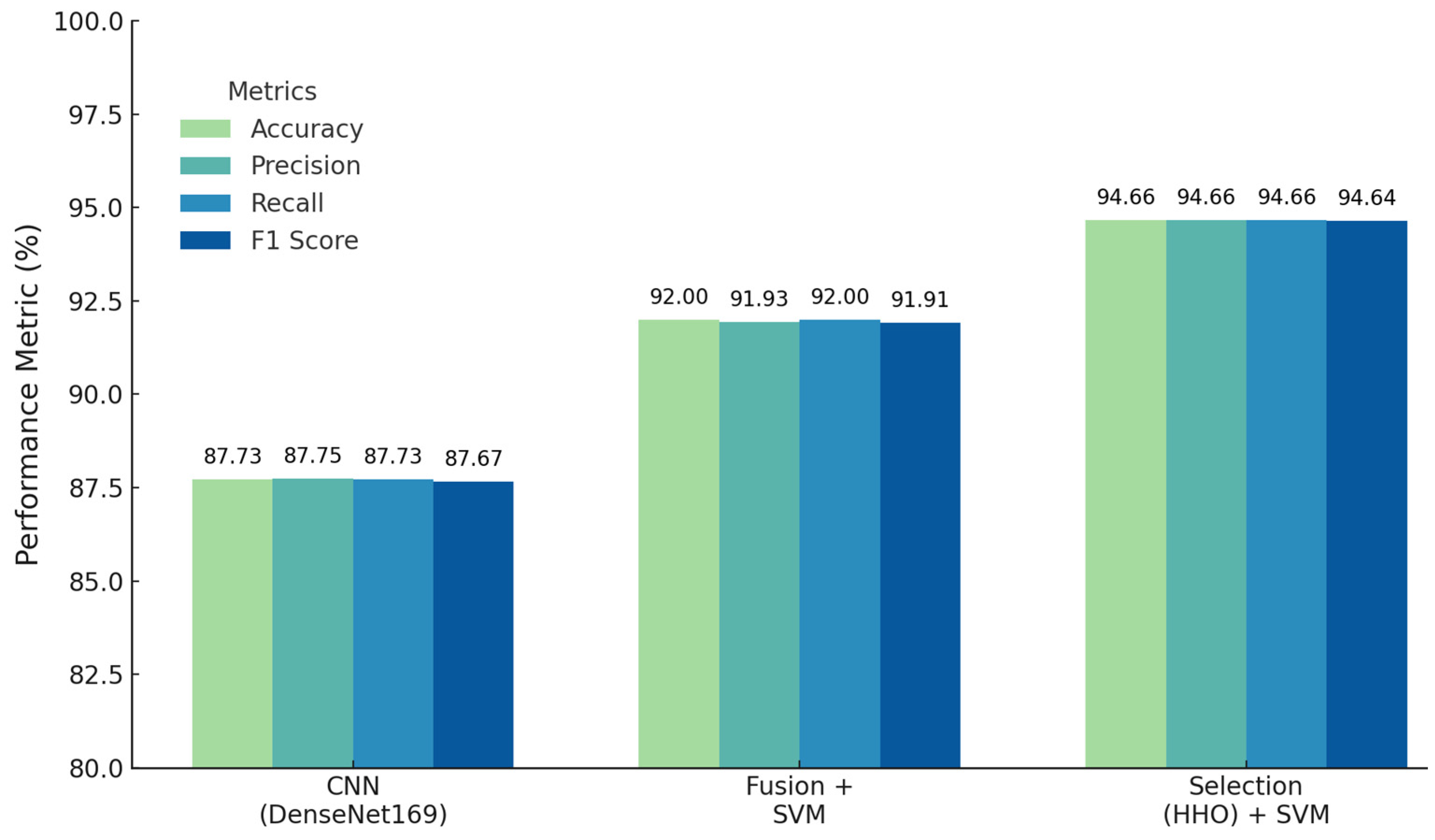
| Feature Selection (HHO) | 94.66 | 94.66 | 94.66 | 94.64 | 0.9286 |
Disclaimer/Publisher’s Note: The statements, opinions and data contained in all publications are solely those of the individual author(s) and contributor(s) and not of MDPI and/or the editor(s). MDPI and/or the editor(s) disclaim responsibility for any injury to people or property resulting from any ideas, methods, instructions or products referred to in the content. |
© 2025 by the authors. Licensee MDPI, Basel, Switzerland. This article is an open access article distributed under the terms and conditions of the Creative Commons Attribution (CC BY) license (https://creativecommons.org/licenses/by/4.0/).
Share and Cite
Şüyun, S.B.; Yurdakul, M.; Taşdemir, Ş.; Biliş, S. Triple-Stream Deep Feature Selection with Metaheuristic Optimization and Machine Learning for Multi-Stage Hypertensive Retinopathy Diagnosis. Appl. Sci. 2025, 15, 6485. https://doi.org/10.3390/app15126485
Şüyun SB, Yurdakul M, Taşdemir Ş, Biliş S. Triple-Stream Deep Feature Selection with Metaheuristic Optimization and Machine Learning for Multi-Stage Hypertensive Retinopathy Diagnosis. Applied Sciences. 2025; 15(12):6485. https://doi.org/10.3390/app15126485
Chicago/Turabian StyleŞüyun, Süleyman Burçin, Mustafa Yurdakul, Şakir Taşdemir, and Serkan Biliş. 2025. "Triple-Stream Deep Feature Selection with Metaheuristic Optimization and Machine Learning for Multi-Stage Hypertensive Retinopathy Diagnosis" Applied Sciences 15, no. 12: 6485. https://doi.org/10.3390/app15126485
APA StyleŞüyun, S. B., Yurdakul, M., Taşdemir, Ş., & Biliş, S. (2025). Triple-Stream Deep Feature Selection with Metaheuristic Optimization and Machine Learning for Multi-Stage Hypertensive Retinopathy Diagnosis. Applied Sciences, 15(12), 6485. https://doi.org/10.3390/app15126485