Research on Predicting Joint Rotation Angles Through Mechanomyography Signals and the Broad Learning System

Abstract

To address the limitation of current upper limb rehabilitation exoskeletons—where pattern recognition-based assistance disrupts patients’ continuous motion—this study proposes a mechanomyography-based model for predicting shoulder and elbow joint angles. Small contact microphones were employed to collect mechanomyography signals, leveraging their ability to capture vibration signals above 8 Hz, making them ideal for mechanomyography acquisition. After extracting raw mechanomyography data, a bandpass filter (10–50 Hz) was applied to eliminate low- and high-frequency noise. To reduce computational overhead during model training, a Broad Learning System was adopted, which iteratively refines predictions by incrementally expanding nodes in the feature and enhancement layers rather than adding hidden layers. The Slime Mold Algorithm was further used to optimize hyperparameters of the Broad Learning System, enhancing prediction accuracy. Experimental results demonstrate that mechanomyography signals exhibit a typical central frequency range of 10–50 Hz, and the Slime Mold Algorithm-optimized Broad Learning System model achieved a minimum coefficient of determination (R²) of 0.978, effectively predicting arm joint angles. This approach shows promise for exoskeletons, combining high control accuracy, real-time joint angle prediction, and computational efficiency.

1. Introduction

In recent years, wearable exoskeletons and robotic limbs have gained widespread adoption across industrial, service, and medical rehabilitation fields, serving to reduce physical strain and restore mobility [1,2]. Often described as a “third hand” or “third leg,” these assistive devices enhance human capabilities by providing supplementary support for demanding tasks [3,4]. However, seamless integration with users requires precise synchronization—exoskeletons must align with human biomechanics, while robotic limbs must accurately interpret motion intent. Consequently, research in human motion intention recognition has become crucial, encompassing pattern classification, joint kinematics prediction, and end-point trajectory analysis [5,6]. The critical significance of continuous motion prediction for rehabilitation exoskeletons lies in enhancing the spatiotemporal coherence of motion control [7]. Through temporal neural networks, continuous motion prediction captures the dynamic temporal features of signals, achieving a leap from discrete action recognition to continuous joint angle prediction. For instance, in exoskeletons, predictive algorithms can anticipate swing trajectories in advance, enabling the exoskeleton to adjust torque output beforehand and avoid motion stuttering caused by traditional discrete control [7]. This forward-looking control in the time dimension reduces the phase difference between assistance and human motion rhythm, significantly lowering energy consumption during movement.

According to recent research [8], MMG, sEMG, inertial sensors, and ultrasound have all been applied to the research on human motion intention perception. The following is an introduction and comparison of them. MMG captures low-frequency mechanical vibration signals (2–150 Hz) generated during muscle contraction using accelerometers or microphones. It offers high signal-to-noise ratio, strong resistance to electromagnetic interference, and the ability to collect signals through clothing. Its advantage lies in directly reflecting mechanical changes in muscles, making it suitable for dynamic motion monitoring, though it has lower spatial resolution. sEMG records muscle electrical activity signals (frequency range: 20–500 Hz) on the skin surface, containing rich neural control information. However, it is susceptible to electrode placement, variations in skin impedance, and electromagnetic interference, requiring direct skin contact. Its strength is high temporal resolution, making it ideal for fine motion recognition, but signal stability is relatively poor. Inertial sensors (accelerometers, gyroscopes) measure limb motion states by detecting acceleration and angular velocity, offering real-time performance and non-contact operation. However, they cannot directly reflect muscle activity and suffer from cumulative errors. They are suitable for navigation and motion trajectory analysis but require integration with other modalities to improve accuracy. Ultrasound uses high-frequency sound waves to image muscle morphology and dynamic changes, enabling the observation of deep muscle structures. However, it has high equipment costs, poor portability, and relies on operator expertise. When combined with sEMG, it can provide complementary morphological information about muscles.

Recent studies have increasingly focused on human motion intention recognition using physiological signals, among which mechanomyography (MMG) has emerged as a prominent modality. MMG signals, which capture muscle contraction-induced vibrations, exhibit a strong correlation with human movement dynamics. For instance, Seongbin An et al. developed a wearable hand gesture recognition system based on pneumatic MMG (pMMG) for direct wrist tendon monitoring, achieving 98.12% accuracy—surpassing conventional sEMG systems (93.89%) [9]. Similarly, P. Wattanasiri et al. proposed a gesture recognition framework combining Continuous Wavelet Transform (CWT) feature extraction with a Domain-Adversarial CNN (DACNN), reporting accuracies of 87.43% (same-posture) and 64.29% (different-posture), which improved to 92.32% and 71.75%, respectively, when extending the MMG window from 200 ms to 600 ms [10]. Further advancing this field, Yongjun Shi et al. leveraged the Hilbert–Huang Transform (HHT) and random forest regression to estimate joint torque from MMG signals, enabling precise control of rehabilitation exosuits [11]. Complementing these efforts, Talib et al. demonstrated significant correlations (p < 0.05) between forearm anthropometrics, MMG root-mean-square values, and flexion torque, highlighting MMG’s potential for muscle activation and size prediction [12].

From recent research, it can be found that both MMG and surface electromyography (sEMG) signals are signals generated by muscle contraction, and they have some differences and connections. MMG measures the vibrational characteristics of muscles, while sEMG detects the electrical activity associated with muscle activation; MMG monitors the mechanical changes during muscle contraction, whereas sEMG tracks the timing of muscle activation; MMG has a lower frequency than sEMG, requiring a lower sampling frequency; and MMG sensors are more convenient to wear compared to sEMG sensors, as they do not require skin preparation or adhesive attachment.

In recent studies, there were three main types of MMG acquisition methods: one was with an accelerometer, one was with a microphone, and the other was with a new piezoelectric sensor or piezoresistive sensor. Jingyu Quan et al. developed high-sensitivity acceleration sensors to detect vibrations that are >10 dB smaller than those detected by conventional commercial sensors. They were the first to measure high-frequency micro-vibrations in muscle fibers, termed micro MMG in patients with Parkinson’s disease (PwPD), using a high-sensitivity acceleration sensor [13]. Soonjae Ahn et al. investigated the relationship of the accelerometer mass and the MMG signal. When the accelerometer mass increased from 8 g to 13 g, the amplitude of the MMG signal increased the most, and the MF of the MMG signal decreased the most. However, for accelerometers heavier than 13 g, no significant change was observed in both the amplitude and MF [14]. Anna Jaskólska et al. compared MMG recorded by a condenser microphone (MIC) and an accelerometer (ACC) during submaximal isometric, concentric, and eccentric contractions in 14 males. The results showed that the information contained in microphone- and accelerometer-based MMG signals is different despite similar trends. It can be concluded that at low-moderate movement velocity, concentric contractions can be investigated by means of an accelerometer and microphone [15]. C. Sebastian Mancero Castillo et al. introduced a new mode of MMG signal capture for enhancing the performance of human–machine interfaces (HMIs) through the modulation of normal pressure at the sensor location. Utilizing this novel approach, increased MMG signal resolution is enabled by a tunable degree of freedom normal to the microphone–skin contact area [16]. Mateusz Szumilas presented a new design of an MMG sensor, which consists of two coupled piezoelectric disks in a single housing. The sensor’s functionality was verified in two experimental setups related to typical MMG applications: an estimation of the force/MMG relationship under static conditions and a neural network-based gesture classification [17]. Cheng-Tang Pan et al. developed a new type of fiber-based MMGmsensor, which was used as a motion on/off trigger sensor for a lower limb rehabilitation exoskeleton (LLRE). Piezoelectric material, polyvinylidene difluoride (PVDF), was applied to fabricate an MMG sensor, using the near-field electrospinning technology to electrically spin PVDF fibers to 5–10 μm in diameter. PVDF fibers attached on an interdigitated (IDT) electrode with different pole pairs and interspaces were packaged into an MMG sensor. This MMG sensor was stuck on the thigh muscles to detect and acquire human motion intention signal, then trigger the controller and actuate the LLRE [18]. Fang Q et al. developed an MMG sensor using a flexible piezoresistive MMG signal sensor based on a pyramidal polydimethylsiloxane (PDMS) microarray sprayed with carbon nanotubes (CNTs). The experiment was conducted, and the results show that the sensitivity of the sensor can reach 0.4 kPa⁻¹ in the measurement range of 0~1.5 kPa, and the correlation reached 96% [19]. Esposito D et al. developed a new, simple, non-invasive sensor based on a force-sensitive resistor (FSR), which is able to measure muscle contraction. The sensor, applied on the skin through a rigid dome, senses the mechanical force exerted by the underlying contracting muscles. In addition to the larger contraction signal, the sensor was able to detect the MMG. The frequency response of the FSR sensor was found to be large enough to correctly measure the MMG. Simultaneous recordings from flexor carpi ulnaris showed a high correlation (Pearson’s r > 0.9) between the FSR output and the MMG linear envelope [20].

From recent research, it can be found that the three acquisition methods have their own advantages and disadvantages. The MMG signal collected by the accelerometer is highly accurate, but it is easily interfered by gravity acceleration and limb movement acceleration; the MMG signal collected by the microphone is not interfered by gravity acceleration and limb movement acceleration, but the influence of environmental noise cannot be ignored; the new piezoelectric and piezoresistive materials are highly comfortable to wear and have high acquisition accuracy, but the material preparation is complex, which makes it difficult to obtain the material and ultimately leads to a high cost of the sensor.

Recent advances in human activity recognition have demonstrated the effectiveness of time-series regression algorithms in analyzing body sensor data, particularly for joint torque and angle prediction. Christopher Caulcrick et al. compared EMG and MMG sensing modalities for assist-as-needed lower-limb exoskeleton (LLE) control, showing that MMG achieves slightly lower torque prediction accuracy than EMG in isometric conditions (94.8 ± 0.7% vs. 97.6 ± 0.8% with neural networks) but comparable performance in dynamic exercises [21]. For joint angle estimation, Chen J et al. developed a deep belief network (DBN)-based regression model using multichannel MMG signals, reducing the RMSE of lower-limb flexion/extension angles by 50% compared to PCA-based methods during walking [22]. Similarly, Coker J et al. employed an artificial neural network to predict knee flexion angles during gait, revealing that prediction accuracy significantly degraded with longer time horizons (p < 0.001), with the RMSE increasing from 0.68° (50 ms) to 4.62° (200 ms) [23]. Hondo N further enhanced dynamic motion analysis by combining MMG with low-frequency acceleration signals (<6 Hz) for knee joint torque estimation. Using Support Vector Regression (SVR), this approach improved the coefficient of determination in healthy subjects and reduced the RMSE during closed kinetic chain (CKC) motions, such as walking-to-standing transitions and chair rises [24].

Despite the progress made, there are still some challenges. Differences in human anatomy and kinematics make it complex to create a universal model, variations in the wearing position can lead to changes in the collected signals, and there are also differences in the signals collected from different individuals; environmental factors such as electromagnetic interference and temperature can affect sensor performance, and non-invasive sensors, such as sEMG sensors based on dry electrodes and MMG sensors based on microphones, are convenient to wear but are susceptible to external noise.

According to previous studies, although sEMG is the standard method for evaluating muscle activation, MMG also has its unique advantages. In this study, in order to construct a human joint motion angle prediction model based on muscle physiological signals, the MMG signal rather than the sEMG signal was selected as the input signal for the angle prediction model. In this study, the small contact microphones were used to measure MMG signals. Compared with microphones, the data collected by small contact microphones were more stable, with stronger anti-noise capabilities and stronger resistance to electromagnetic interference; compared with the accelerometer, the data collected by small contact microphones were not be affected by gravity acceleration and limb movement acceleration, and compared with the new piezoelectric sensor or piezoresistive sensor, small contact microphones are readily available and inexpensive. What’s more, a novel method for predicting joint rotation angles based on the Broad Learning System (BLS) [25,26] was proposed, and the model hyperparameters were optimized using the Slime Mold Algorithm (SMA) [27]. The implementation of the SMA-BLS algorithm significantly improved the generalization ability of the joint angle prediction model while enhancing the training efficiency.

2. Materials and Methods

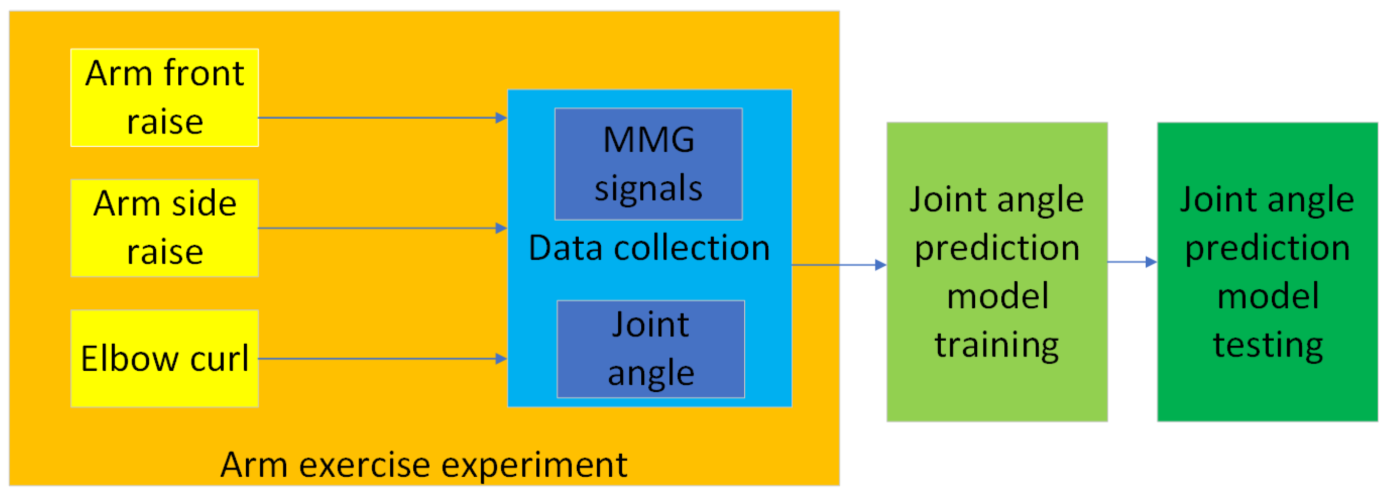
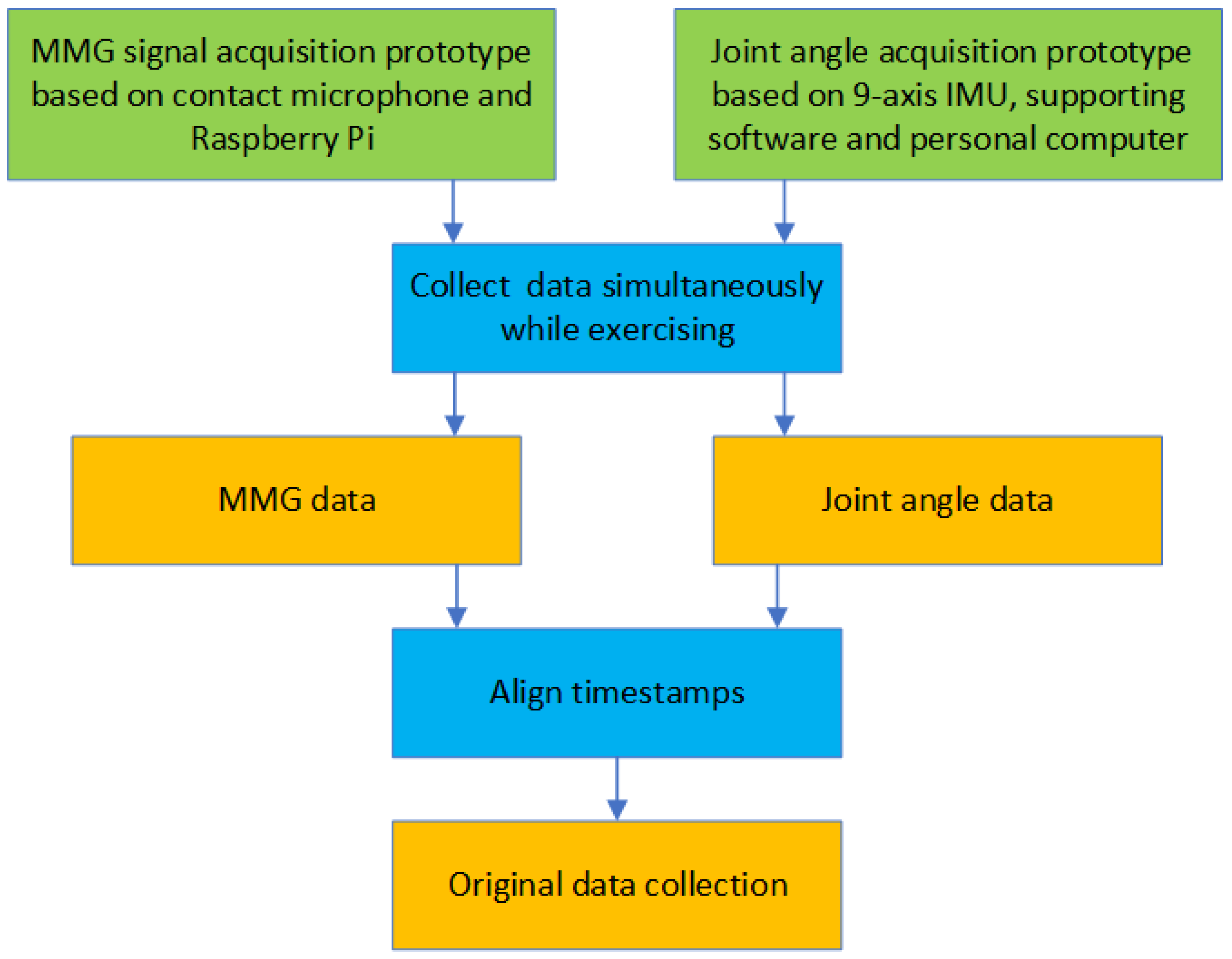
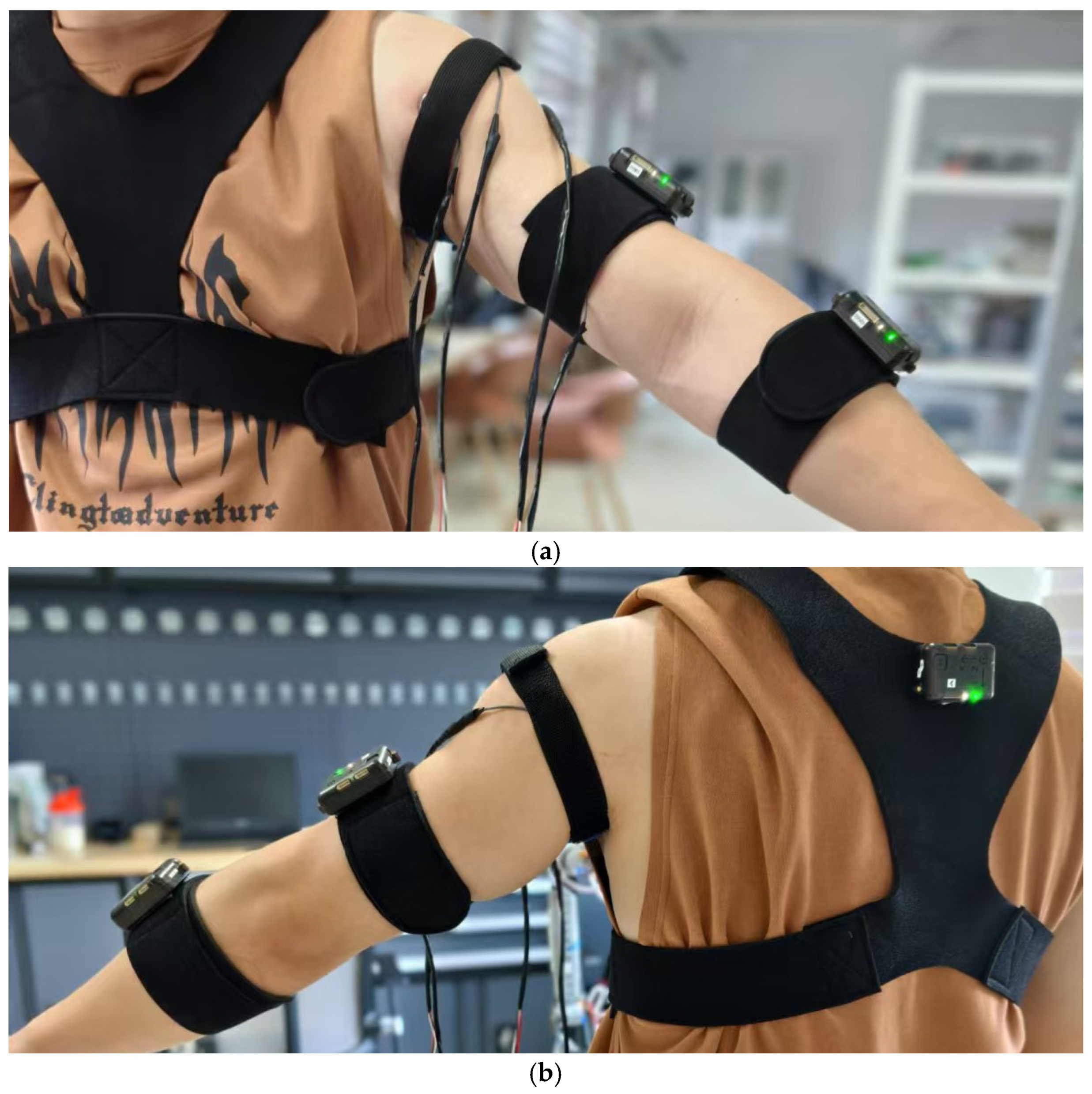
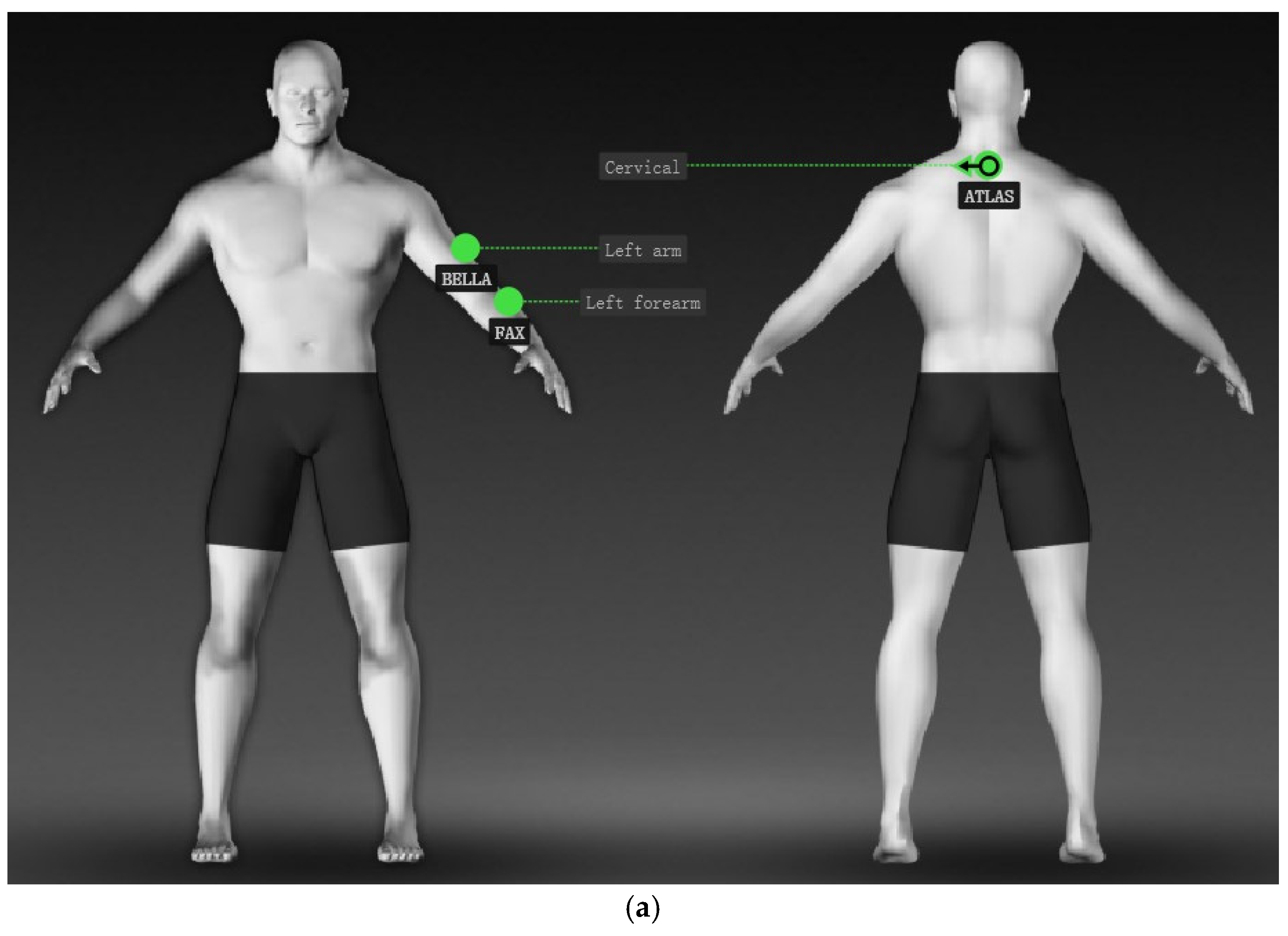
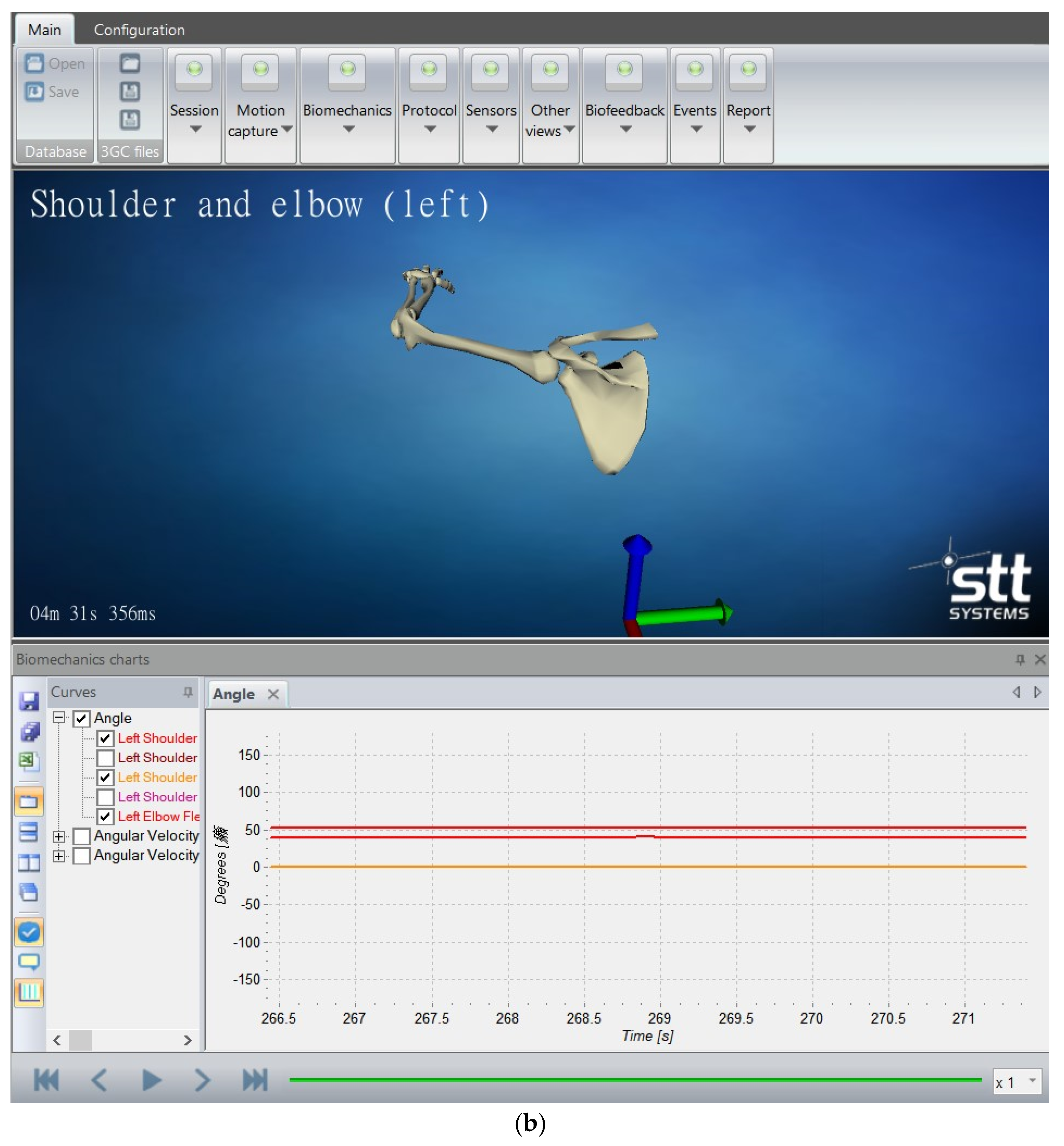
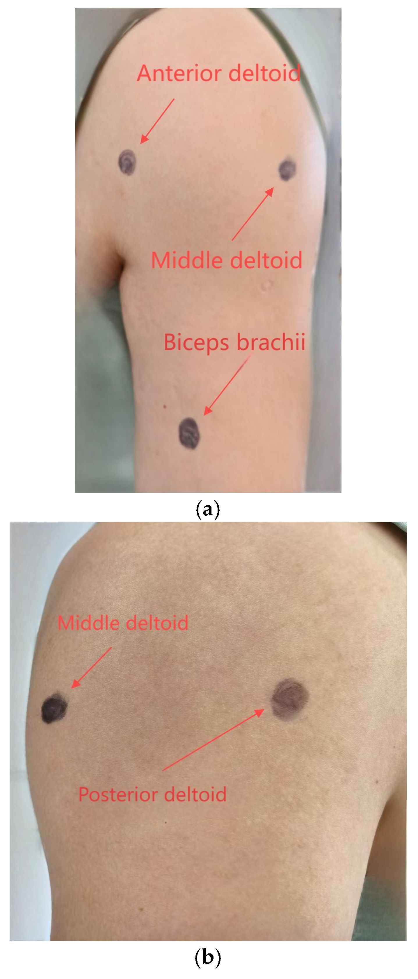
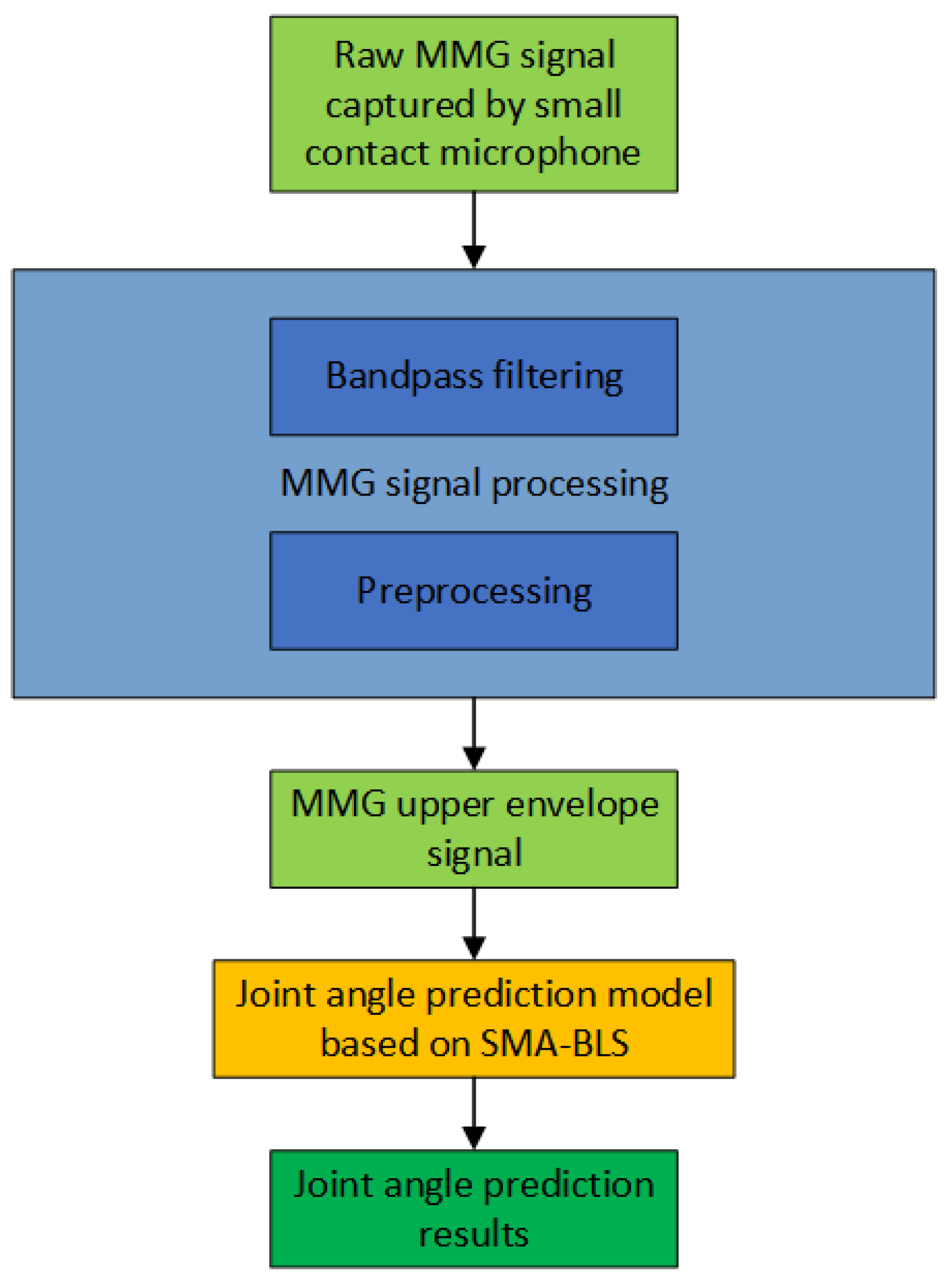
2.1. Experimental Process

The experiment lasted for four days, from 2 January 2024 to 5 January 2024. During this period, relevant data were collected for research purposes. The author had access to the participants’ identifiable information both during and after the data collection phase. A total of 12 volunteers participated in this study. All the subjects were school students, aged between 24 and 30 years old. The height was between 174.3 and 185.6 cm, weight was between 75.6 and 92.8 KG, and body mass index was between 21.3 and 25.9. Before the experiment began, all participants were fully informed about the research objectives, procedures, and potential risks. Written informed consent was obtained from each participant prior to the implementation of the experimental protocol.

Figure 1 is the flowchart of the experiment and research. In this study, participants were required to perform three specific upper limb movements at a constant speed: arm forward raise, bicep curl, and arm lateral raise. To ensure consistency in movement execution, participants were instructed to maintain a steady and controllable rhythm throughout the exercise. During the exercise, small contact microphones were attached to the skin over the anterior deltoid, medial deltoid, posterior deltoid, and the biceps brachii to record the MMG signals. To enhance the amplitude and quality of the MMG signals, participants were required to hold a dumbbell during the exercise. This additional load was chosen to increase muscle activation within a safe and manageable range for all participants. The weight of the dumbbells was 0.5 KG and 1 KG, and finally the prescribed movements are completed without dumbbells. Three load conditions were compared to determine whether changes in muscle activation due to varying loads could improve the accuracy of the model in predicting joint angles. Heavier dumbbells were not used, as greater weights might cause muscles to fatigue too quickly, leading to significant changes in the characteristics of the MMG signals and a substantial reduction in the accuracy of the model’s joint angle predictions. This is not the main focus of the current study. A metronome was used to guide participants to maintain a constant speed, set at 30 beats per minute, to ensure consistency across all trials and participants. For each subject, a total of 60 min of data were collected for each exercise, among them, 20 min of data are without load, 20 min of data are with load of 0.5 KG, and 20 min of data are with load of 1KG. During the subject’s exercise, the subject rested for one minute after every one minute of exercise, and no data were collected during the rest period. This research aims to focus on joint angle prediction using MMG signals in non-fatigued states, as fatigue causes significant alterations in MMG signal characteristics, which would substantially reduce the model’s generalization performance and significantly increase training costs. According to previous studies [28], one minute of low-intensity exercise will not cause muscle fatigue, and the characteristics of muscle sound signals will not change significantly. The fatigue status of the subjects was recorded throughout the collection process. During the experiment, no subject felt obvious fatigue.

Figure 2 is a schematic diagram of data collection during the experiment. The MMG signal is continuously recorded by a data acquisition system with a sampling rate of 400 Hz. Joint angles are measured by multiple inertial measurement units (IMUs) with a sampling rate of 200 Hz. The MMG signal is a signal generated by muscle contraction and precedes joint movement, so it can be used for joint angle prediction [29,30]. However, the IMU data are synchronous with joint movement, compared with IMU data, MMG signals are more suitable for joint angle prediction.

In this study, the MMG signal was collected by small contact microphones, which are shown in Figure 3. Contact microphones are not affected by ambient noise, nor by gravity or body movement acceleration; therefore, it is suitable for measuring MMG data related to human motion research. The contact sensor is first connected to the signal amplification module. The signal amplification module has a built-in Butterworth bandpass filter circuit, and the filtered MMG signal was transmitted to a Raspberry Pi. The MMG signal acquisition prototype is shown in Figure 4.

In this study, 9-axis inertial measurement units (IMUs) were used to record the angle of joints throughout the movement process. The appearance of the IMU is shown in Figure 5. The IMU integrates a tri-axis accelerometer, gyroscope, and magnetometer, providing powerful functionality for tracking comprehensive motion dynamics. The 9-axis IMU sensor has matching data processing software, which can convert the data of the IMU sensor into human joint angle data. The positions of the IMU and the small contact microphones are shown in Figure 6, the interface of the data processing software is shown in Figure 7, the connection of the joint angle acquisition prototype is shown in Figure 8.

During the data collection process, scripts control the collection process of MMG data and joint angle data, and the simultaneity of the two data collections was confirmed using timestamps. Since the purpose of this study was to use MMG signals to predict joint angles, MMG signals were used to estimate joint angles as a function of their temporal characteristics after a certain time interval, the time interval ranges from 10 ms, 30 ms, to 60 ms. In previous studies [31], sEMG signals were used to predict joint angles, and the time in the future was set to 50 ms. Considering that MMG is not more ahead of human movement than sEMG, the time in the future used in this study is not much larger than 50 ms. As the time in the future increases, the prediction error gradually increases, and excessive prediction errors will cause the angle prediction to lose its practical value. Therefore, the maximum time in the future of 60 ms used in this study is reasonable. In addition, in order to compare the impact of different time in the future on prediction accuracy, two parameters, 10 ms and 30 ms, were selected to compare with 60 ms.

After bandpass filtering, the MMG signal underwent a series of preprocessing steps [31], which runs on the Raspberry Pi, as delineated below:

(1)

Full-wave rectification;

(2)

Upper envelope signal extraction.

To accurately locate the muscle bellies of each head of the biceps brachii and the deltoid, two anatomical landmarks were selected as reference points, and palpation was used for confirmation [32]. Figure 9 is a schematic diagram of the muscle belly position. The long head of the biceps brachii originates from the supraglenoid tubercle of the scapula. The short head originates from the coracoid process of the scapula. Its insertion is at the radial tuberosity anterior to the elbow joint, which is the tendon insertion point of the biceps brachii. The palpation steps are as follows: Ask the subject to flex the elbow and perform a slight supination movement. At this time, the biceps brachii will contract noticeably. Use fingers to slide along the anterior side of the upper arm from the shoulder to the elbow, the protruding muscle tissue is the muscle belly of the biceps brachii. The muscle belly is usually located at the middle of the upper arm, about one-third to one-half of the distance from the elbow joint.

The anterior deltoid originates from the lateral third of the clavicle. Its insertion is at the deltoid tuberosity of the humerus. The palpation steps are as follows: Locate the lateral end of the clavicle and use hand to slide along the clavicle towards the shoulder to determine the position of the lateral third of the clavicle. Ask the subject to perform shoulder flexion or internal rotation. At this time, the anterior deltoid will contract. Use fingers to press downward from the lateral end of the clavicle, the protruding muscle tissue is the muscle belly of the anterior deltoid. The muscle belly is usually located near the shoulder joint, below the clavicle.

The middle deltoid originates from the acromion. Its insertion is at the deltoid tuberosity of the humerus. The palpation steps are as follows: Locate the acromion. Ask the subject to perform shoulder abduction. At this time, the middle deltoid will contract noticeably. Use fingers to slide outward from the acromion, the bulging muscle tissue is the muscle belly of the middle deltoid. The muscle belly is usually located laterally to the acromion, near the lateral side of the upper arm.

The posterior deltoid originates from the posterior surface of the spine of the scapula. Its insertion is at the deltoid tuberosity of the humerus. The palpation steps are as follows: Locate the posterior surface of the spine of the scapula. Ask the subject to perform shoulder extension or external rotation. At this time, the posterior deltoid will contract. Use fingers to slide outward from the posterior surface of the spine of the scapula, the tense muscle tissue is the muscle belly of the posterior deltoid. The muscle belly is usually located posterior to the spine of the scapula, near the posterior side of the upper arm. After confirming the locations of the muscle bellies of the four muscles, mark the most prominent positions of each muscle belly with a pen for subsequent analysis and training guidance.

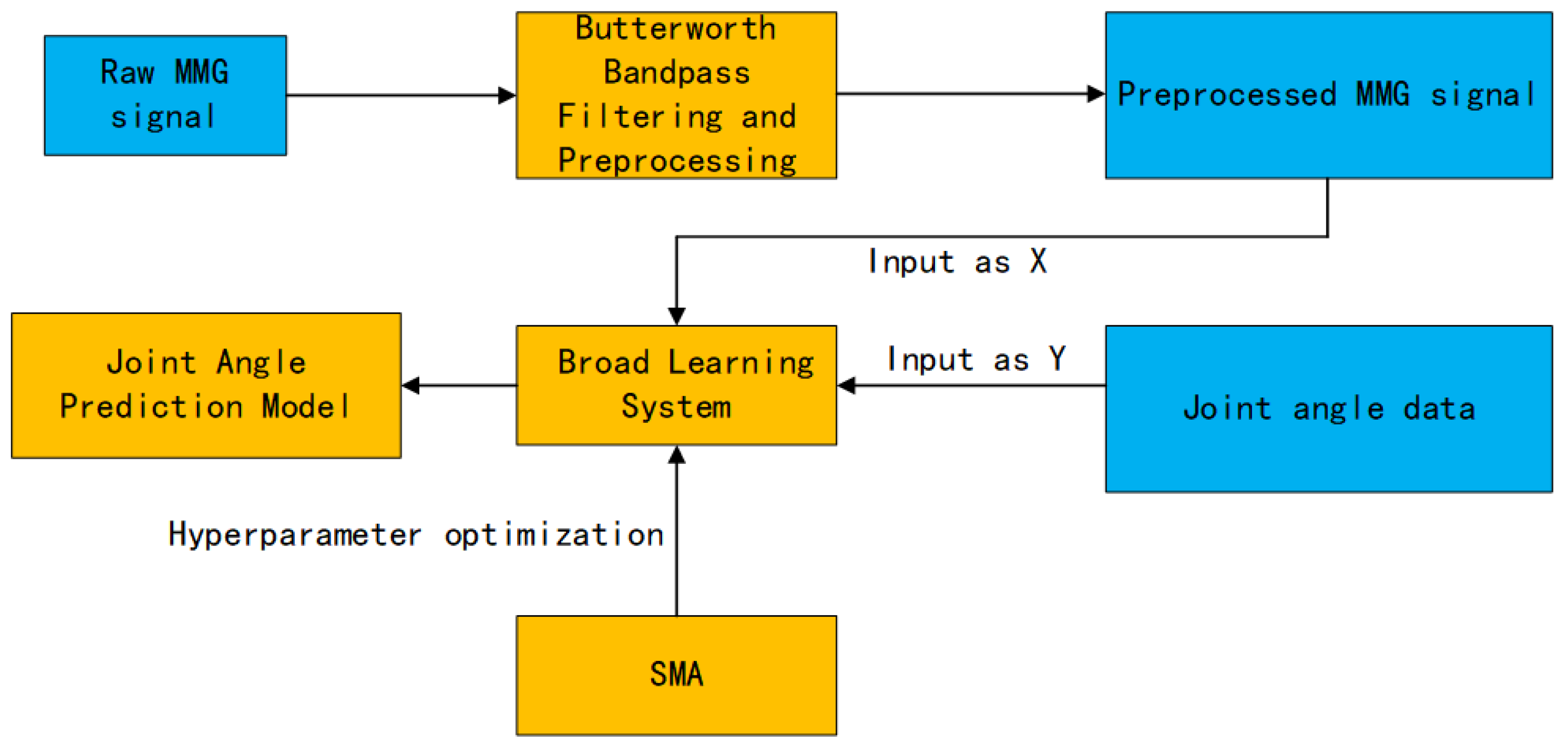
2.2. Human Joint Rotation Angle Estimation Model Based on SMA-BLS

In this research, the Broad Learning System (BLS) was utilized for human joint angle prediction, and the Slime Mold Algorithm (SMA) was utilized for optimization of hyperparameters in BLS.

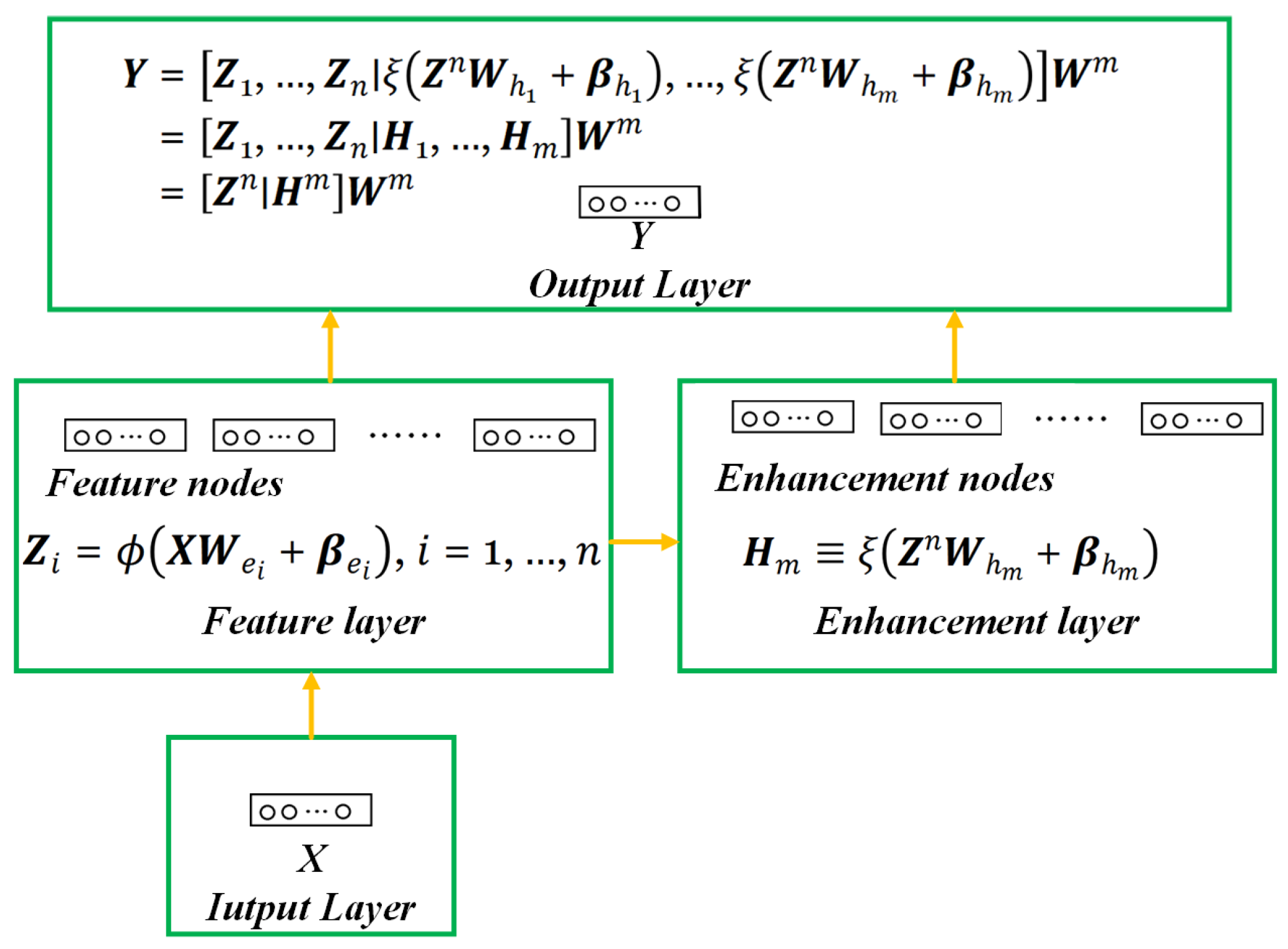
2.2.1. Broad Learning System

The Broad Learning System (BLS) (Algorithm 1) represents an innovative machine learning architecture, introduced as a substitute for conventional deep learning methodologies. Its primary objectives are to streamline the complexity of the model structure and to expedite the training phase. The hypothesis was introduced by a team of investigators from Guangdong University of Technology in the year 2017. The BLS has been architected to deliver elevated performance across diverse computational tasks such as classification, regression, and clustering. Notably, it accomplishes this with a substantial reduction in computational resource demands, in contrast to the more intensive requirements of deep neural networks. The pseudo code of the BLS is shown in Figure 10. The structure of the BLS is shown in Figure 10. The following is the pseudo code of the BLS.

Algorithm 1 Broad Learning System

$\mathrm{Input}\text{:} \mathrm{Raw} \mathrm{MMG} \mathrm{signals} X$$; \mathrm{Joint} \mathrm{angle} \mathrm{data} Y$. $\mathrm{Hyperparameters}\text{:} N$$(\mathrm{feature} \mathrm{nodes}); D$$(\mathrm{projection} \dim ); \lambda$$\left(\mathrm{regularization}\right) \mathrm{Trained} \mathrm{weights} Beta$. $\mathrm{Output}\text{:} \mathrm{Predicted} \mathrm{values} \widehat{Y}.$ (1) Data Preparation: Extract upper envelope MMG via preprocessing $\mathrm{Combine} \mathrm{envelopes} \mathrm{to} \mathrm{form} \mathrm{input} \mathrm{matrix} X$ (2) Initialize Feature Nodes: $\mathrm{Generate} \mathrm{random} \mathrm{projection} \mathrm{matrix} W\in {\mathbb{R}}^{d\times D}$ $\mathrm{Compute} \mathrm{feature} \mathrm{nodes}\text{:} Z\leftarrow X\cdot W$ (3) Generate Enhancement Nodes: $\mathrm{Create} \mathrm{random} \mathrm{weights} W_e$$\mathrm{and} \mathrm{bias} {\beta }_e$ $\mathrm{Compute} \mathrm{nonlinear} \mathrm{transform}\text{:} E\leftarrow \xi (Z\cdot W_e+{\beta }_e)$ $\mathrm{Concatenate} \mathrm{features}\text{:} H\leftarrow [Z\mid E]$ (4) Ridge Regression: $\mathrm{Compute} \mathrm{regularized} \mathrm{weights}\text{:} Beta\leftarrow (H^{T}H+\lambda I{)}^{-1}{H}^{T}Y$ (5) Training & Prediction: Training: $\mathrm{Store} H$$\mathrm{and} Beta$ $\mathrm{Prediction} \mathrm{for} \mathrm{new} X_{\mathrm{new}}$: $Z_{\mathrm{new}}\leftarrow X_{\mathrm{new}}\cdot W$ $E_{\mathrm{new}}\leftarrow \xi (Z_{\mathrm{new}}\cdot W_e+{\beta }_e)$ $H_{\mathrm{new}}\leftarrow [Z_{\mathrm{new}}\mid E_{\mathrm{new}}]$ $\widehat{Y}\leftarrow H_{\mathrm{new}}\cdot Beta$ (6) Incremental Learning: If New data available  $W^{\mathrm{\prime }}\leftarrow \mathrm{random}\text{\_}\mathrm{init}\left(\right)$  $Z^{\mathrm{\prime }}\leftarrow X_{\mathrm{new}}\cdot W^{\mathrm{\prime }}$  $H\leftarrow [H\mid Z^{\mathrm{\prime }}]$  $\mathrm{Update} Beta$ End if If Performance insufficient  $E^{\mathrm{\prime }}\leftarrow \xi (Z\cdot W_{e^{\mathrm{\prime }}}+{\beta }_{e^{\mathrm{\prime }}})$  $H\leftarrow [H\mid E^{\mathrm{\prime }}]$  $\mathrm{Recalculate} Beta\leftarrow (H^{T}H+\lambda I{)}^{-1}{H}^{T}Y$ End if

2.2.2. Slime Mold Algorithm

The Slime Mold Algorithm (SMA) (Algorithm 2) constitutes a metaheuristic optimization technique inspired by natural processes, specifically emulating the foraging and adaptive behavior exhibited by slime mold. The algorithm was initially proposed by Li et al. The algorithm, developed in 2020, has garnered significant interest due to its demonstrated efficiency and efficacy in addressing a diverse array of optimization challenges. The following is the pseudo code of the SMA.

Algorithm 2 Slime Mold Algorithm

$\mathrm{Input}\text{:} \mathrm{Population} \mathrm{size} N$$; \mathrm{Max} \mathrm{iterations} T$$; \mathrm{Search} \mathrm{space} \mathrm{boundaries} [lb,ub]$$; \mathrm{Objective} \mathrm{function} f\left(X\right)$. $\mathrm{Output}\text{:} \mathrm{Global} \mathrm{best} \mathrm{solution} X_{\mathrm{best}}$$; \mathrm{Best} \mathrm{fitness} \mathrm{value} f_{\mathrm{best}}$. (1) Initialization: $X_i\leftarrow lb+\mathrm{rand}\left(\right)\times (ub-lb)$ $\mathrm{Initialize} \mathrm{dynamic} \mathrm{parameter} a$ $\mathrm{Set} \mathrm{probability} \mathrm{threshold} z$ for random exploration (2) Fitness Evaluation: ${\mathrm{fitness}}_i\leftarrow f\left(X_i\right)$ $X_{\mathrm{best}}\leftarrow \mathrm{a}\mathrm{r}\mathrm{g}\mathrm{m}\mathrm{i}\mathrm{n}\left(\mathrm{fitness}\right)$ $f_{\mathrm{best}}\leftarrow f\left(X_{\mathrm{best}}\right)$ $\left(3\right) \mathrm{Main} \mathrm{Loop} (t=1$$\mathrm{to} T$): $\mathrm{Update} a\leftarrow 1-(t/T)$ If rand() < z then $X_i^{t+1}\leftarrow lb+\mathrm{rand}\left(\right)\times (ub-lb)$ else $r_1\leftarrow \mathrm{uniform}\text{\_}\mathrm{random}\left[\mathrm{0,1}\right]$ $r_2\leftarrow \mathrm{uniform}\text{\_}\mathrm{random}[-\mathrm{1,1}]$ $X_i^{t+1}\leftarrow X_i^t+r_1\times (X_{\mathrm{best}}^t-|X_i^t\left|\right)\times r_2$ Boundary Handling: $\mathrm{If} X_i^{t+1}$$> ub$ $X_i^{t+1}\leftarrow ub$ $\mathrm{If} X_i^{t+1}$$< lb$ $X_i^{t+1}\leftarrow lb$ Fitness Re-evaluation: $\mathrm{Update} {\mathrm{fitness}}_i\leftarrow f\left(X_i\right)$ $\mathrm{Update} X_{\mathrm{best}}$$\mathrm{and} f_{\mathrm{best}}$ if better solution found (4) Termination: $\mathrm{Return} X_{\mathrm{best}}$$\mathrm{and} f_{\mathrm{best}}$$\mathrm{when} t=T$ or convergence criteria met

2.2.3. Role of SMA in BLS Parameter Optimization

(1)

Global Search:

The SMA efficiently searches large solution spaces to find near-optimal parameters for BLS, such as the number of feature nodes and projection dimensions.

(2)

Local Fine-Tuning:

After finding good solutions, the SMA refines them further, improving the model’s performance through precise adjustments.

(3)

Avoid Premature Convergence:

The SMA prevents getting stuck in suboptimal solutions by dynamically adjusting its search strategy, leading to better results.

Advantages of Using SMA for BLS Parameter Optimization

(1)

Flexibility:

The SMA works well with various types of optimization problems, including those without gradient information or highly nonlinear functions, making it ideal for complex models like the BLS.

(2)

Efficiency:

The SMA is computationally efficient, finding good solutions quickly, which is especially useful for large datasets and high-dimensional parameter spaces.

(3)

Ease of Use:

The SMA is simple to understand and implement, making it easy to integrate into existing machine learning frameworks.

(4)

Improved Performance:

By optimizing BLS parameters, the SMA enhances the model’s accuracy, stability, and ability to generalize, leading to better practical outcomes.

(5)

Robustness:

The SMA handles noisy data and uncertainties effectively, providing reliable optimization even in challenging conditions.

The structure of human joint angle prediction method is shown in Figure 11. The joint angle prediction model training process is shown in Figure 12. The process of real-time prediction of joint angle is shown in Figure 13.

3. Results

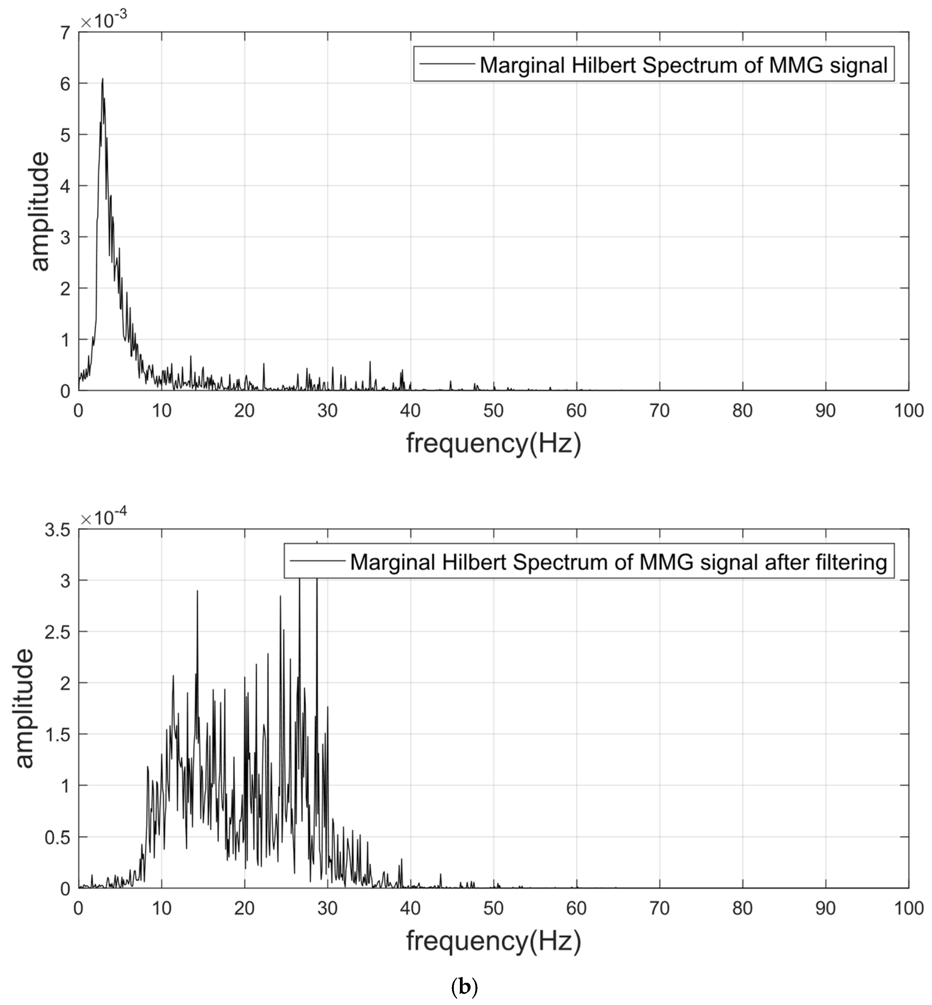
3.1. The Results of Butterworth Bandpass Filtering of the MMG Signal

Taking the results of the raw signals of the biceps brachii during the curling exercise as an example, Figure 14 illustrate the results of Butterworth Bandpass Filtering of the MMG signal. There was a bandpass filter circuit on the signal amplification module of the sensor. The passband of the bandpass filter is 10–50 Hz [33]. After being processed by the Butterworth bandpass filter, the low-frequency and high-frequency noise in the original MMG signal are removed, which is well shown in the spectrum in Figure 14b. The Marginal Hilbert Spectrum is a two-dimensional representation derived from the Hilbert spectrum; it shows the total energy contribution of each frequency value. The Marginal Hilbert Spectrum helps us understand the energy distribution of different frequencies in a signal [34,35].

3.2. The Results of Preprocessing the MMG Signal

Figure 15 illustrates the MMG signal after bandpass processing and the MMG signal after preprocessing, which was used as an example to illustrate the effect of preprocessing, and the results for other muscles were similar to this example. The graphical representation clearly demonstrated that the MMG signals, with significant fluctuation characteristics, were converted into a more regular and stationary form following the preprocessing procedure. The joint angle prediction model based on the upper envelope signal of MMG is easier to train and has higher accuracy than the prediction model based on the MMG signal [31].

3.3. The Results of Joint Angle Prediction

This study used a dataset containing data from 12 people. This study studied three specific upper limb movements, so there are three datasets in total. Each dataset is divided into six parts. This study employed a six-fold cross-validation scheme to ensure the robustness and reliability of the model training results. For each fold, five of the six segments were used as the training set, while the remaining sixth segment was used as the test set. The model was trained on the training set and subsequently evaluated using the corresponding test set. Performance metrics, including the mean squared error (MSE), root mean squared error (RMSE), mean absolute error (MAE), and coefficient of determination (R²), were obtained for each fold. The training and testing process was repeated six times, with each segment serving as the test set once. After completing the six iterations, the final performance metrics were obtained by calculating the average of the results from each fold. This approach not only comprehensively evaluated the model’s performance but also minimized the bias and variance introduced by single train-test splits. After completing the model training, the model was used to realize the real-time prediction of joint angles, and the RMSE was used to evaluate the results of the model’s real-time prediction.

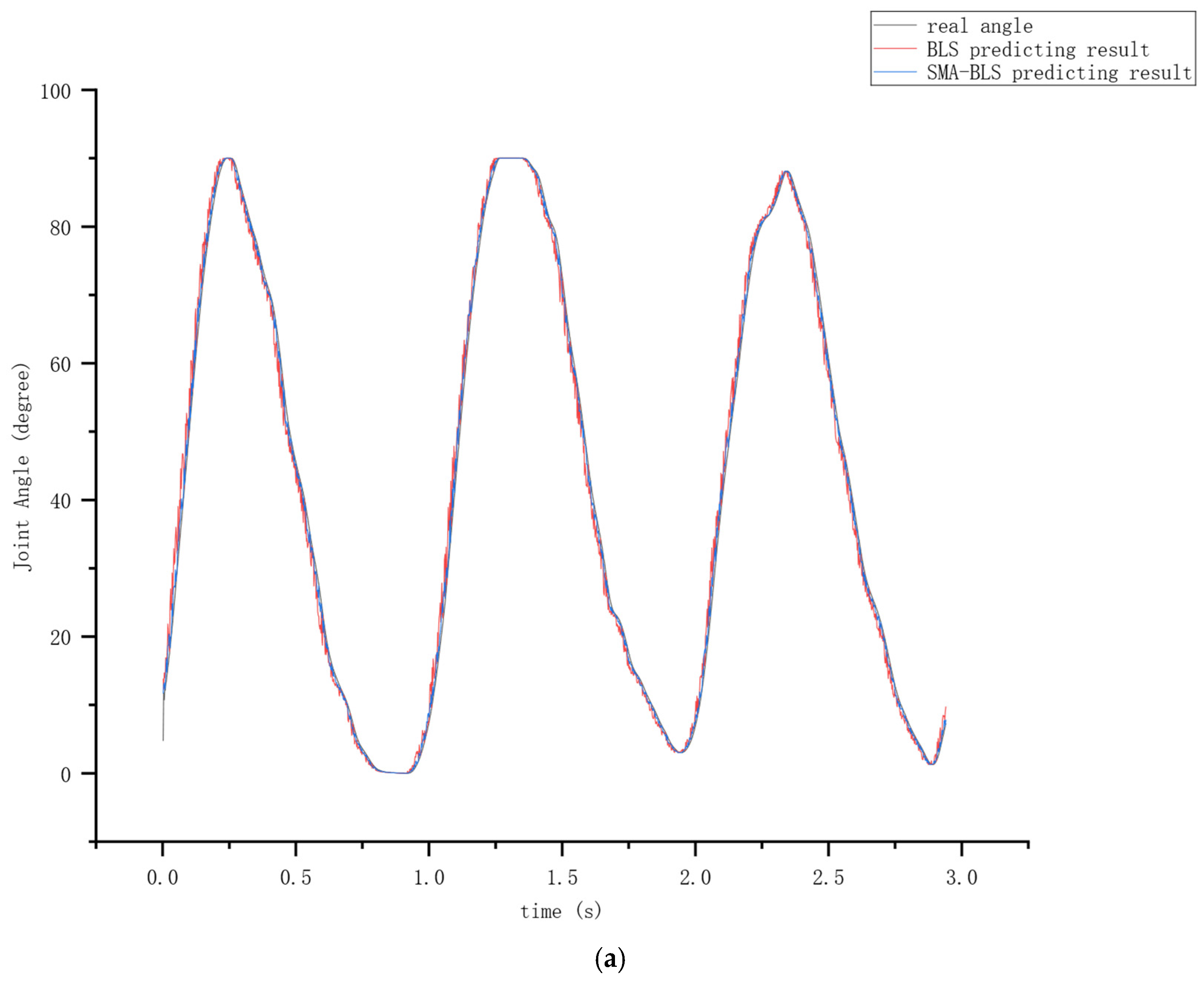
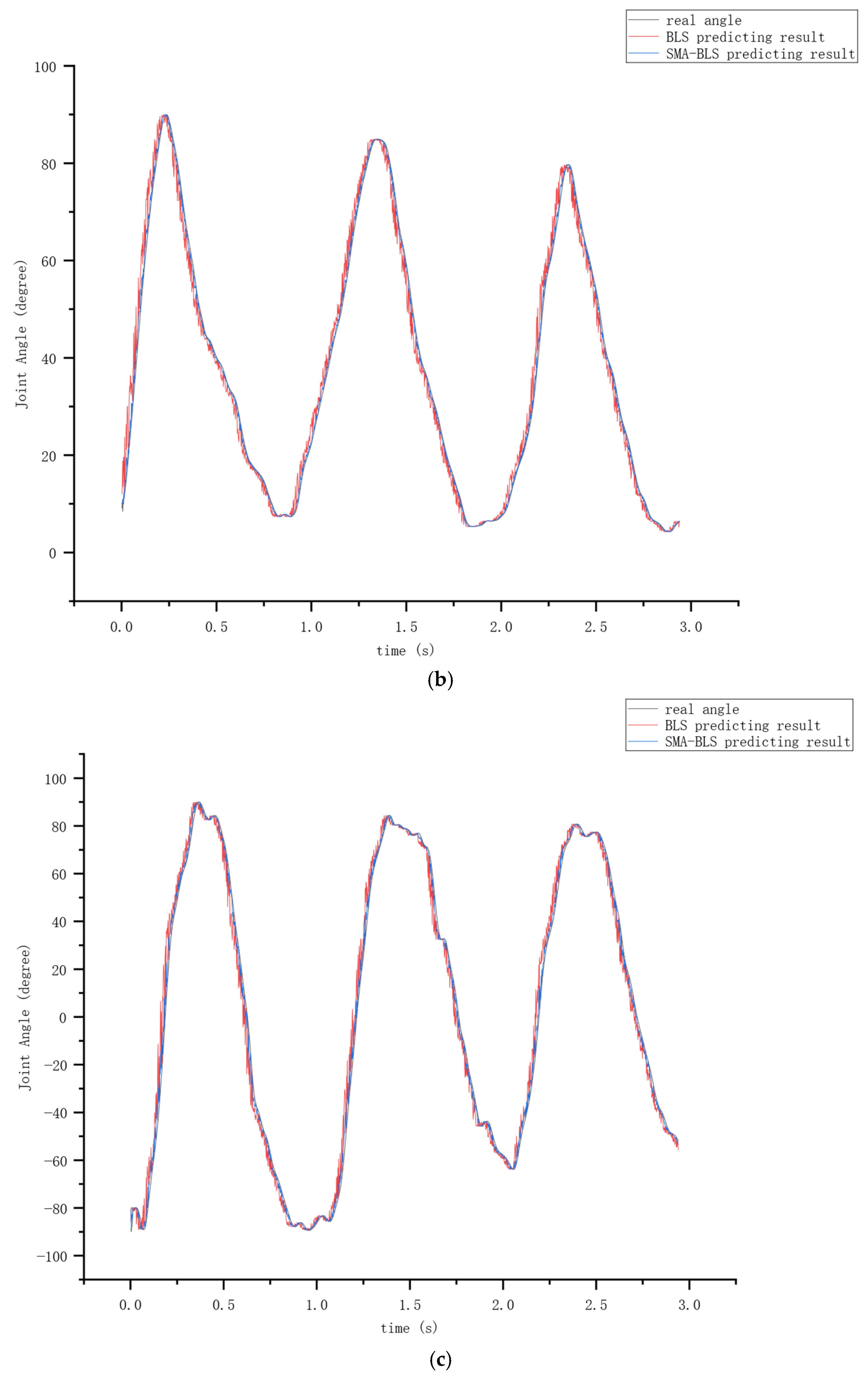
3.3.1. The Impact of the SMA on the Prediction Results

In this research, a total of three upper limb movements were taken as research objects, including arm front raise, arm side raise, and elbow curl. In the arm front raise and arm side raise, the shoulder joint angle is the object to be predicted, and in the arm curl, the elbow joint angle is the object to be predicted.

Table 1. (a) Best parameters of shoulder joint angle prediction results during arm side raises. (b) Best parameters of shoulder joint angle prediction results during arm front raises. (c) Best parameters of shoulder joint angle prediction results during elbow curls. (d) Parameters of SMA.

(a)
Parameters	Value
L2 regularization parameters and enhanced node reduction ratio	0.959
Number of windows in feature layer	52
Number of feature nodes per window in feature layer	51
Number of nodes in the enhancement layer	199
(b)
Parameters	Value
L2 regularization parameters and enhanced node reduction ratio	0.958
Number of windows in feature layer	53
Number of feature nodes per window in feature layer	51
Number of nodes in the enhancement layer	200
(c)
Parameters	Value
L2 regularization parameters and enhanced node reduction ratio	0.960
Number of windows in feature layer	52
Number of feature nodes per window in feature layer	51
Number of nodes in the enhancement layer	202
(d)
Parameters	Value
Population number	10
Maximum number of iterations	20
Objective function	MSE
Bottom of search area	[0.01, 10, 10, 10]
Top of search area	[1, 100, 100, 300]

reveals the refined parameters of the BLS and the parameters of the SMA. L2 regularization parameters and enhanced node reduction ratio, the number of windows in feature layer, number of feature nodes per window in feature layer, and number of nodes in the enhancement layer were hyperparameters of the BLS which were optimized by the SMA. The model was trained using data from subjects with no load on their hands, and the time in the future was 10 ms.

Table 2. (a) Prediction results of BLS and SMA-BLS during arm side raise. (b) Prediction results of BLS and SMA-BLS during arm front raise. (c) Prediction results of BLS and SMA-BLS during elbow curl.

(a)
Method	MSE	RMSE	MAE	R2	p-Value
SMA-BLS	$0.0019 \pm$0.0001	$0.0366 \pm$0.0012	$0.0098 \pm$0.0006	$0.970 \pm$0.002	/
BLS	$0.0046 \pm$0.0002	$0.0658 \pm$0.0021	$0.0564 \pm$0.0025	$0.937 \pm$0.004	0.0077
(b)
Method	MSE	RMSE	MAE	R2	p-Value
SMA-BLS	$0.0020 \pm$0.0001	$0.0387 \pm$0.0009	$0.0108 \pm$0.0007	$0.963 \pm$0.001	/
BLS	$0.0051 \pm$0.0004	$0.0677 \pm$0.0033	$0.0587 \pm$0.0027	$0.931 \pm$0.004	0.0086
(c)
Method	MSE	RMSE	MAE	R2	p-Value
SMA-BLS	$0.0021 \pm$0.0001	$0.0402 \pm$0.0010	$0.0119 \pm$0.0006	$0.959 \pm$0.002	/
BLS	$0.0062 \pm$0.0004	$0.0734 \pm$0.0032	$0.0631 \pm$0.0021	$0.929 \pm$0.003	0.0084

shows the results of model training. Table 2 confirms the SMA-BLS’s exceptional predictive precision. Notably, for collective datasets, the peak metrics were MSE = 0.0019, RMSE = 0.0366, MAE = 0.0098, and R² = 0.970. Table 2 further highlights the SMA’s proficiency in fine-tuning BLS hyperparameters, markedly elevating prediction reliability. To evaluate whether there is a statistically significant difference in the R² between the SMA-BLS and BLS, two-sample T-test was employed. According to Table 2, the p-value were significantly lower than the commonly accepted level (α = 0.02). This indicated that there was strong evidence to suggest that there was a statistically significant difference in the mean accuracy rates between the SMA-BLS and BLS.

Figure 16 delineates the results of predicting in real time. During arm side raises, the RMSE of shoulder joint angle prediction based on the SMA-BLS was 0.0418; during arm front raises, the RMSE of shoulder joint angle prediction based on the SMA-BLS was 0.0441; during elbow curls, the RMSE of the elbow joint angle prediction based on the SMA-BLS was 0.0485.

3.3.2. Prediction Results of Different Input Signals

In order to verify the superiority of the MMG signal, the rotation angle data collected by the IMU were also used to predict joint angles. The rotation angle data of the IMU located at the forearm were used to predict the joint angle of elbow joint, and the rotation angle data of the IMU located at the upper arm was used to predict the joint angle of shoulder joint.

Table 3. (a) Prediction results of different input signals during arm side raises. (b) Prediction results of different input signals during arm front raises. (c) Prediction results of different input signals during elbow curls.

(a)
Input Signals	MSE	RMSE	MAE	R2	p-Value
MMG	$0.0019 \pm$0.0001	$0.0366 \pm$0.0012	$0.0098 \pm$0.0006	$0.970 \pm$0.002	/
IMU rotation angle	$0.0052 \pm$0.0003	$0.0701 \pm$0.0019	$0.0531 \pm$0.0036	$0.941 \pm$0.005	0.0065
(b)
Input signals	MSE	RMSE	MAE	R2	p-Value
MMG	$0.0020 \pm$0.0001	$0.0387 \pm$0.0009	$0.0108 \pm$0.0007	$0.963 \pm$0.001	/
IMU rotation angle	$0.0054 \pm$0.0003	$0.0768 \pm$0.0026	$0.0695 \pm$0.0037	$0.936 \pm$0.003	0.0053
(c)
Input signals	MSE	RMSE	MAE	R2	p-Value
MMG	$0.0021 \pm$0.0001	$0.0402 \pm$0.0010	$0.0119 \pm$0.0006	$0.959 \pm$0.002	/
IMU rotation angle	$0.0059 \pm$0.0002	$0.0831 \pm$0.0036	$0.0683 \pm$0.0026	$0.926 \pm$0.002	0.0041

shows the results of training. The findings revealed that the prediction accuracy of MMG is higher.

Experiments on real-time prediction of joint angles were also conducted. During arm side raises, the RMSE of shoulder joint angle prediction result was 0.0631 and 0.0842, respectively; during arm front raises, the RMSE of shoulder joint angle prediction result was 0.0593 and 0.0776, respectively; during elbow curls, the RMSE of elbow joint angle prediction result was 0.0579 and 0.0791, respectively. In all three exercises, the prediction errors based on MMG are much smaller than those based on the IMU.

3.3.3. Prediction Results of Different Times in the Future

Table 4. (a) Prediction results of different times in the future during arm side raises. (b) Prediction results of different times in the future during arm front raises. (c) Prediction results of different times in the future during elbow curls.

(a)
Time in the Future (ms)	MSE	RMSE	MAE	R2
10	$0.0019 \pm$0.0001	$0.0366 \pm$0.0012	$0.0098 \pm$0.0006	$0.970 \pm$0.002
30	$0.0032 \pm$0.0002	$0.0588 \pm$0.0017	$0.0297 \pm$0.0021	$0.941 \pm$0.003
60	$0.0056 \pm$0.0003	$0.0691 \pm$0.0023	$0.0491 \pm$0.0027	$0.934 \pm$0.002
(b)
Time in the Future(ms)	MSE	RMSE	MAE	R2
10	$0.0020 \pm$0.0001	$0.0387 \pm$0.0009	$0.0108 \pm$0.0007	$0.963 \pm$0.001
30	$0.0034 \pm$0.0002	$0.0499 \pm$0.0018	$0.0346 \pm$0.0022	$0.938 \pm$0.003
60	$0.0064 \pm$0.0004	$0.0681 \pm$0.0024	$0.0506 \pm$0.0036	$0.931 \pm$0.003
(c)
Time in the Future(ms)	MSE	RMSE	MAE	R2
10	$0.0021 \pm$0.0001	$0.0402 \pm$0.0010	$0.0119 \pm$0.0006	$0.959 \pm$0.002
30	$0.0036 \pm$0.0003	$0.0592 \pm$0.0031	$0.0374 \pm$0.0023	$0.937 \pm$0.003
60	$0.0058 \pm$0.0003	$0.0706 \pm$0.0033	$0.0594 \pm$0.0041	$0.929 \pm$0.003

is the result of model training. Table 4 delineates the predicting results of different times in the future. The findings reveal that the increase in time in the future leads to a decrease in prediction accuracy.

Experiments on real-time prediction of joint angles were also conducted. During arm side raises, the RMSE of shoulder joint angle prediction result was 0.0418, 0.0599, and 0.0735, respectively, when the prediction time was 10 ms, 30 ms, and 60 ms; during arm front raises, the RMSE of the shoulder joint angle prediction result was 0.0441, 0.0605, and 0.0748, respectively, when the prediction time was 10 ms, 30 ms, and 60 ms; during elbow curls, the RMSE of elbow joint angle prediction result was 0.0485, 0.0634, and 0.0780, respectively, when the prediction time was 10 ms, 30 ms, and 60 ms.

3.3.4. Prediction Results of Different Loads

Table 5. (a) Prediction results of different loads during arm side raises. (b) Prediction results of different loads during arm front raises. (c) Prediction results of different loads during elbow curls.

(a)
Load Weight (KG)	MSE	RMSE	MAE	R2
0	$0.0019 \pm$0.0001	$0.0366 \pm$0.0012	$0.0098 \pm$0.0006	$0.970 \pm$0.002
0.5	$0.0017 \pm$0.0001	$0.0342 \pm$0.0011	$0.0090 \pm$0.0005	$0.974 \pm$0.001
1	$0.0015 \pm$0.0001	$0.0324 \pm$0.0010	$0.0083 \pm$0.0005	$0.978 \pm$0.001
(b)
LoadWeight (KG)	MSE	RMSE	MAE	R2
0	$0.0020 \pm$0.0001	$0.0387 \pm$0.0009	$0.0108 \pm$0.0007	$0.963 \pm$0.001
0.5	$0.0018 \pm$0.0001	$0.0365 \pm$0.0009	$0.0094 \pm$0.0005	$0.970 \pm$0.002
1	$0.0016 \pm$0.0001	$0.0346 \pm$0.0008	$0.0089 \pm$0.0004	$0.974 \pm$0.001
(c)
LoadWeight (KG)	MSE	RMSE	MAE	R2
0	$0.0021 \pm$0.0001	$0.0402 \pm$0.0010	$0.0119 \pm$0.0006	$0.959 \pm$0.002
0.5	$0.0019 \pm$0.0001	$0.0378 \pm$0.0010	$0.0101 \pm$0.0005	$0.964 \pm$0.002
1	$0.0016 \pm$0.0001	$0.0350 \pm$0.0009	$0.0092 \pm$0.0005	$0.969 \pm$0.001

delineates that as the weight of the load on the subject’s hand increased, the accuracy of joint angle prediction improved to a certain extent. This was because the load increased the degree of muscle contraction, thereby increasing the amplitude of the MMG signal, which ultimately led to an improvement in the accuracy of joint angle prediction.

Experiments on real-time prediction of joint angles were also conducted. The results illustrate that when the hand load increases within a certain range, the prediction accuracy of the joint angle increases. However, if the load level increases further, it may cause rapid muscle fatigue, resulting in a decrease in prediction accuracy. During arm side raise, the RMSE of the shoulder joint angle prediction result was 0.0418, 0.0394, and 0.0368, respectively, when the subject’s hand load was 0, 0.5 and 1 KG; during arm front raises, the RMSE of the shoulder joint angle prediction result was 0.0441, 0.0409, and 0.0376, respectively, when the subject’s hand load was 0, 0.5, and 1 KG; during elbow curls, the RMSE of the elbow joint angle prediction result was 0.0485, 0.0443, and 0.0408, respectively, when the subject’s hand load was 0, 0.5, and 1 KG.

3.3.5. Prediction Results of Different Forecast Methods

The comparative analysis which was shown in

Table 6. (a) Prediction results of different algorithms during arm side raises. (b) Prediction results of different algorithms during arm front raises. (c) Prediction results of different algorithms during elbow curls.

(a)
Method	MSE	RMSE	MAE	R2	p-Value	Training Time (s)	Forecast Time (ms)
SMA-BLS	$0.0019 \pm$0.0001	$0.0366 \pm$0.0012	$0.0098 \pm$0.0006	$0.970 \pm$0.002	/	174.3 ± 5.36	4.1 ± 0.32
CNN	$0.0041 \pm$0.0003	$0.0689 \pm$0.0015	$0.0694 \pm$0.0026	$0.932 \pm$0.002	0.00760	259.2 ± 13.67	21.4 ± 2.41
SVM	$0.0044 \pm$0.0002	$0.0728 \pm$0.0013	$0.0762 \pm$0.0027	$0.926 \pm$0.003	0.00519	336.6 ± 11.94	19.8 ± 2.63
BP	$0.0053 \pm$0.0003	$0.0788 \pm$0.0025	$0.0869 \pm$0.0048	$0.919 \pm$0.004	0.00218	95.6 ± 2.67	11.6 ± 1.80
ELM	$0.0048 \pm$0.0003	$0.0668 \pm$0.0011	$0.0709 \pm$0.0016	$0.923 \pm$0.002	0.00308	135.5 ± 5.19	16.3 ± 2.24
RF	$0.0058 \pm$0.0003	$0.0887 \pm$0.0024	$0.0908 \pm$0.0034	$0.909 \pm$0.002	0.00143	168.3 ± 6.95	26.5 ± 1.31
RBF	$0.0042 \pm$0.0003	$0.0619 \pm$0.0026	$0.0669 \pm$0.0031	$0.916 \pm$0.002	0.00394	195.3 ± 6.74	13.9 ± 1.08
LSTM	$0.0039 \pm$0.0002	$0.0597 \pm$0.0011	$0.0686 \pm$0.0014	$0.936 \pm$0.003	0.00821	267.4 ± 8.18	14.2 ± 1.94
(b)
Method	MSE	RMSE	MAE	R2	p-Value	Training Time (s)	Forecast Time (ms)
SMA-BLS	$0.0020 \pm$0.0001	$0.0387 \pm$0.0009	$0.0108 \pm$0.0007	$0.963 \pm$0.001	/	176.6 ± 5.44	4.2 ± 0.27
CNN	$0.0043 \pm$0.0002	$0.0679 \pm$0.0014	$0.0699 \pm$0.0016	$0.931 \pm$0.001	0.00760	257.8 ± 13.16	20.1 ± 2.32
SVM	$0.0041 \pm$0.0003	$0.0736 \pm$0.0012	$0.0746 \pm$0.0023	$0.925 \pm$0.004	0.00497	337.7 ± 10.58	19.2 ± 2.56
BP	$0.0056 \pm$0.0003	$0.0759 \pm$0.0027	$0.0832 \pm$0.0035	$0.918 \pm$0.003	0.00196	98.3 ± 2.57	10.9 ± 1.73
ELM	$0.0045 \pm$0.0004	$0.0691 \pm$0.0013	$0.0716 \pm$0.0021	$0.924 \pm$0.002	0.00321	138.2 ± 5.11	16.7 ± 2.15
RF	$0.0057 \pm$0.0003	$0.0896 \pm$0.0026	$0.0942 \pm$0.0025	$0.910 \pm$0.003	0.00137	169.6 ± 6.82	26.3 ± 1.24
RBF	$0.0045 \pm$0.0004	$0.0608 \pm$0.0021	$0.0618 \pm$0.0029	$0.912 \pm$0.003	0.00364	194.2 ± 6.63	13.8 ± 1.14
LSTM	$0.0038 \pm$0.0002	$0.0588 \pm$0.0012	$0.0662 \pm$0.0013	$0.937 \pm$0.002	0.00842	262.6 ± 8.08	14.3 ± 1.84
(c)
Method	MSE	RMSE	MAE	R2	p-Value	Training Time (s)	Forecast Time (ms)
SMA-BLS	$0.0021 \pm$0.0001	$0.0402 \pm$0.0010	$0.0119 \pm$0.0006	$0.959 \pm$0.002	/	185.3 ± 15.48	4.2 ± 0.95
CNN	$0.0046 \pm$0.0003	$0.0702 \pm$0.0019	$0.0748 \pm$0.0028	$0.928 \pm$0.002	0.00705	258.6 ± 6.42	19.9 ± 2.18
SVM	$0.0048 \pm$0.0003	$0.0735 \pm$0.0014	$0.0774 \pm$0.0026	$0.923 \pm$0.004	0.00451	339.4 ± 9.18	19.3 ± 2.26
BP	$0.0052 \pm$0.0002	$0.0709 \pm$0.0016	$0.0806 \pm$0.0034	$0.920 \pm$0.003	0.00308	97.6 ± 2.06	11.1 ± 1.96
ELM	$0.0043 \pm$0.0002	$0.0652 \pm$0.0012	$0.0663 \pm$0.0014	$0.927 \pm$0.002	0.00275	137.9 ± 4.96	16.9 ± 2.14
RF	$0.0061 \pm$0.0004	$0.0906 \pm$0.0032	$0.0985 \pm$0.0038	$0.903 \pm$0.004	0.00096	169.0 ± 5.99	25.6 ± 1.06
RBF	$0.0046 \pm$0.0002	$0.0687 \pm$0.0029	$0.0703 \pm$0.0033	$0.905 \pm$0.002	0.00169	194.5 ± 5.96	13.3 ± 1.64
LSTM	$0.0040 \pm$0.0001	$0.0632 \pm$0.0008	$0.0673 \pm$0.0010	$0.938 \pm$0.003	0.00806	266.8 ± 8.06	14.2 ± 1.65

reveals that the SMA-BLS algorithm exhibited superior efficiency and boasted enhanced prediction accuracy when contrasted with other algorithms evaluated. Table 6 illustrates the comparative outcomes of various prediction methodologies utilizing multi-person datasets, with the SMA-BLS algorithm exhibiting superior performance in terms of prediction accuracy and computational efficiency. To evaluate whether there is a statistically significant difference in the R² between SMA-BLS and other algorithms, a two-sample T-test was employed. According to Table 6, the p-values were significantly lower than the commonly accepted level (α = 0.02).

4. Discussion

This study proposed an upper limb joint angle prediction method based on small contact microphones and the SMA-BLS algorithm, which can be used for the control of upper limb rehabilitation exoskeleton.

In this study, small contact microphones were used to collect MMG signals because they are not affected by environmental noise, motion acceleration, or gravity acceleration. Furthermore, the small contact microphone used in this research is inexpensive and suitable for commercialization. After collecting the original MMG signal, the MMG signal was processed using bandpass filtering and preprocessing to remove low- and high-frequency noise and to obtain the upper envelope signal of the MMG signal. This preprocessing process was simple but effective, and it minimized the signal processing time while ensuring signal quality, which also helps it to be applied in practical scenarios. Following that, a novel joint angle prediction method based on the SMA-BLS was applied. The BLS framework exhibited incremental learning capabilities, a flat network structure, fast training speeds, high accuracy, and low computational overhead. The integration of the SMA further enhanced the BLS by leveraging its foraging behavior, adaptability, and self-organization properties, resulting in a high-precision, computationally efficient joint angle prediction method.

From the results, we can find that as time in the future increased, the training accuracy and real-time prediction accuracy of the joint prediction model decreased. In addition, with the increase in the weight of the hand load, the training accuracy and real-time prediction accuracy of the joint prediction model increased. This may be because the load causes the amplitude of the MMG signal to increase, which leads to an increase in the proportion of effective information in the MMG signal, and ultimately leads to an improvement in prediction accuracy. This study did not use a larger load because a larger load may cause the muscles to fatigue too quickly, resulting in an abnormal decrease in prediction accuracy.

The MMG signal technology shows promise in muscle state monitoring, but its accuracy is significantly affected by fatigue levels due to spectral feature drift caused by fatigue. Studies indicate that the spectral characteristics of MMG signals undergo notable changes under fatigue. For instance, while the high-frequency band extends, the proportion of high-frequency energy decreases substantially. Additionally, nonlinear features such as fractal dimension (FD) exhibit a linear decline during fatigue, though with considerable inter-individual variability, further complicating model generalization.

In general, muscle fatigue is an important influencing factor in MMG-based joint angle prediction research, which will also be the focus of the next stage of research.

5. Conclusions

In the present investigation, an innovative methodology was proposed for the prediction of the shoulder and elbow joints angles, leveraging MMG signals in conjunction with the Broad Learning System optimized by the Slime Mold Algorithm (SMA-BLS).

What’s more, the study found that with the increase in time in the future, the training accuracy of the model and the real-time prediction accuracy of the joint angle decreased, but the real-time prediction accuracy of the joint angle of the proposed method can meet the fine angle control requirements of the rehabilitation upper limb exoskeleton. In the subsequent research on the rehabilitation upper limb exoskeleton, the control method considered for application will use the joint angle prediction method proposed in this study. This method uses the MMG signal of an intact arm combined with the contact force signal and the joint motor angle signal to drive the rehabilitation exoskeleton. The purpose is to use the patient’s intact arm to drive the rehabilitation exoskeleton to train the paralyzed arm. The prediction results based on MMG and the IMU have also been compared. The comparison results show that MMG is indeed superior to the IMU, and its prediction accuracy for joint angles under prescribed exercises is better than the IMU.

In addition, the study found that as the hand load increased from 0 to 1 KG, the accuracy of joint angle prediction was significantly improved. This shows that the model proposed in this study can be applied to joint angle prediction in daily behavior, and the model also has broad application prospects in the field of upper limb assisted exoskeleton control. In future research, upper limb assisted exoskeletons based on MMG signals will be developed to freely adjust joint angle prediction model parameters and exoskeleton assistance strategies according to the user’s hand load, thereby reducing the sense of frustration during the assistance process and ultimately achieving precise assistance and smooth control.

In this study, the prediction accuracy of joint angles under loads greater than 1 kg was not tested. This is because excessive loads may cause muscles to quickly enter the fatigue stage, resulting in an abnormal decrease in prediction accuracy. In subsequent studies, joint angle prediction combined with muscle fatigue level identification will also be one of the research focuses, because fatigue is a common condition in human daily activities, and joint angle prediction considering fatigue conditions will have a wider range of application scenarios.

References

1. Vélez-Guerrero, M.A.; Callejas-Cuervo, M.; Mazzoleni, S. Artificial intelligence-based wearable robotic exoskeletons for upper limb rehabilitation: A review. Sensors 2021, 21, 2146. [Google Scholar] [CrossRef] [PubMed]
2. Coser, O.; Tamantini, C.; Soda, P.; Zollo, L. AI-based methodologies for exoskeleton-assisted rehabilitation of the lower limb: A review. Front. Robot. AI 2024, 11, 1341580. [Google Scholar] [CrossRef]
3. Jing, H.; Zheng, T.; Zhang, Q.; Sun, K.; Li, L.; Lai, M.; Zhao, J.; Zhu, Y. Human Operation Augmentation through Wearable Robotic Limb Integrated with Mixed Reality Device. Biomimetics 2023, 8, 479. [Google Scholar] [CrossRef]
4. Miller, L.E.; Zimmermann, A.K.; Herbert, W.G. Clinical effectiveness and safety of powered exoskeleton-assisted walking in patients with spinal cord injury: Systematic review with meta-analysis. Med. Devices Evid. Res. 2016, 9, 455–466. [Google Scholar] [CrossRef]
5. Gu, F.; Chung, M.-H.; Chignell, M.; Valaee, S.; Zhou, B.; Liu, X. A survey on deep learning for human activity recognition. ACM Comput. Surv. (CSUR) 2021, 54, 1–34. [Google Scholar] [CrossRef]
6. Jobanputra, C.; Bavishi, J.; Doshi, N. Human activity recognition: A survey. Procedia Comput. Sci. 2019, 155, 698–703. [Google Scholar] [CrossRef]
7. Plaza, A.; Hernandez, M.; Puyuelo, G.; Garces, E.; Garcia, E. Lower-limb medical and rehabilitation exoskeletons: A review of the current designs. IEEE Rev. Biomed. Eng. 2021, 16, 278–291. [Google Scholar] [CrossRef]
8. Dwivedi, A.; Groll, H.; Beckerle, P. A systematic review of sensor fusion methods using peripheral bio-signals for human intention decoding. Sensors 2022, 22, 6319. [Google Scholar] [CrossRef]
9. An, S.; Feng, J.; Song, E.; Kong, K.; Kim, J.; Choi, H. High-accuracy hand gesture recognition on the wrist tendon group using pneumatic mechanomyography (pMMG). IEEE Trans. Ind. Inform. 2023, 20, 1550–1561. [Google Scholar] [CrossRef]
10. Wattanasiri, P.; Wilson, S.; Huo, W.; Vaidyanathan, R. Gesture Recognition through Mechanomyogram Signals: An Adaptive Framework for Arm Posture Variability. IEEE J. Biomed. Health Inform. 2024, 29, 2453–2462. [Google Scholar] [CrossRef]
11. Shi, Y.; Dong, W.; Lin, W.; He, L.; Wang, X.; Li, P.; Gao, Y. Human joint torque estimation based on mechanomyography for upper extremity exosuit. Electronics 2022, 11, 1335. [Google Scholar] [CrossRef]
12. Talib, I.; Sundaraj, K.; Hussain, J.; Lam, C.K.; Ahmad, Z. Analysis of anthropometrics and mechanomyography signals as forearm flexion, pronation and supination torque predictors. Sci. Rep. 2022, 12, 16086. [Google Scholar] [CrossRef] [PubMed]
13. Quan, J.; Uchitomi, H.; Shigeyama, R.; Gao, C.; Ogata, T.; Inaba, A.; Orimo, S.; Miyake, Y. High-sensitivity acceleration sensor detecting micro-mechanomyogram and deep learning approach for parkinson’s disease classification. Sci. Rep. 2024, 14, 22941. [Google Scholar] [CrossRef]
14. Ahn, S.; Shin, I.; Kim, Y. The effect of accelerometer mass in mechanomyography measurements. J. Vibroeng. 2016, 18, 4736–4742. [Google Scholar] [CrossRef]
15. Jaskólska, A.; Madeleine, P.; Jaskólski, A.; Kisiel-Sajewicz, K.; Arendt-Nielsen, L. A comparison between mechanomyographic condenser microphone and accelerometer measurements during submaximal isometric, concentric and eccentric contractions. J. Electromyogr. Kinesiol. 2007, 17, 336–347. [Google Scholar] [CrossRef] [PubMed]
16. Castillo, C.S.M.; Wilson, S.; Vaidyanathan, R.; Atashzar, S.F. Wearable MMG-plus-one armband: Evaluation of normal force on mechanomyography (MMG) to enhance human-machine interfacing. IEEE Trans. Neural Syst. Rehabil. Eng. 2020, 29, 196–205. [Google Scholar] [CrossRef]
17. Szumilas, M.; Władziński, M.; Wildner, K. A coupled piezoelectric sensor for mmg-based human-machine interfaces. Sensors 2021, 21, 8380. [Google Scholar] [CrossRef]
18. Pan, C.T.; Chang, C.C.; Yang, Y.S.; Yen, C.-K.; Kao, Y.-H.; Shiue, Y.-L. Development of MMG sensors using PVDF piezoelectric electrospinning for lower limb rehabilitation exoskeleton. Sens. Actuators A Phys. 2020, 301, 111708. [Google Scholar] [CrossRef]
19. Fang, Q.; Cao, S.; Qin, H.; Yin, R.; Zhang, W.; Zhang, H. A Novel Mechanomyography (MMG) Sensor Based on Piezo-Resistance Principle and with a Pyramidic Microarray. Micromachines 2023, 14, 1859. [Google Scholar] [CrossRef]
20. Esposito, D.; Andreozzi, E.; Fratini, A.; Gargiulo, G.D.; Savino, S.; Niola, V.; Bifulco, P. A piezoresistive sensor to measure muscle contraction and mechanomyography. Sensors 2018, 18, 2553. [Google Scholar] [CrossRef]
21. Caulcrick, C.; Huo, W.; Hoult, W.; Vaidyanathan, R. Human joint torque modelling with MMG and EMG during lower limb human-exoskeleton interaction. IEEE Robot. Autom. Lett. 2021, 6, 7185–7192. [Google Scholar] [CrossRef]
22. Chen, J.; Zhang, X.; Cheng, Y.; Xi, N. Surface EMG based continuous estimation of human lower limb joint angles by using deep belief networks. Biomed. Signal Process. Control 2018, 40, 335–342. [Google Scholar] [CrossRef]
23. Coker, J.; Chen, H.; Schall, M.C., Jr.; Gallagher, S.; Zabala, M. EMG and joint angle-based machine learning to predict future joint angles at the knee. Sensors 2021, 21, 3622. [Google Scholar] [CrossRef] [PubMed]
24. Hondo, N.; Tsuji, T. Knee Joint Torque Estimation in Femoral Prosthesis Users Using MMG and Low-Frequency Acceleration. IEEE Access 2024, 12, 174996–175005. [Google Scholar] [CrossRef]
25. Gong, X.; Zhang, T.; Chen, C.L.P.; Liu, Z. Research review for broad learning system: Algorithms, theory, and applications. IEEE Trans. Cybern. 2021, 52, 8922–8950. [Google Scholar] [CrossRef]
26. Chen, C.L.P.; Liu, Z. Broad learning system: An effective and efficient incremental learning system without the need for deep architecture. IEEE Trans. Neural Netw. Learn. Syst. 2017, 29, 10–24. [Google Scholar] [CrossRef]
27. Li, S.; Chen, H.; Wang, M.; Heidari, A.A.; Mirjalili, S. Slime mould algorithm: A new method for stochastic optimization. Future Gener. Comput. Syst. 2020, 111, 300–323. [Google Scholar] [CrossRef]
28. Søgaard, K.; Gandevia, S.C.; Todd, G.; Petersen, N.T.; Taylor, J.L. The effect of sustained low-intensity contractions on supraspinal fatigue in human elbow flexor muscles. J. Physiol. 2006, 573, 511–523. [Google Scholar] [CrossRef]
29. Wang, S.; Yang, J.; Yang, H.; Sun, T.; Dong, M.; Hou, Z.G. Prediction of Upper Limb Joint Angles Based on Multi-Source Information Fusion using Temporal Convolutional Network. In Proceedings of the 2024 30th International Conference on Mechatronics and Machine Vision in Practice (M2VIP), Leeds, UK, 3–5 October 2024; pp. 1–6. [Google Scholar]
30. Yao, J.; Xia, C.; Zhang, H.; Zhu, C. Research on the Prediction of Elbow Joint Angle Based on Mechanomyography. In Proceedings of the 2022 IEEE 10th Joint International Information Technology and Artificial Intelligence Conference (ITAIC), Chongqing, China, 17–19 June 2022; Volume 10, pp. 547–553. [Google Scholar]
31. Zhu, M.; Guan, X.; Li, Z.; He, L.; Wang, Z.; Cai, K. sEMG-based lower limb motion prediction using CNN-LSTM with improved PCA optimization algorithm. J. Bionic Eng. 2023, 20, 612–627. [Google Scholar] [CrossRef]
32. Chaurasia, B.D. Human Anatomy; CBS Publisher: New Delhi, India, 2004. [Google Scholar]
33. Meagher, C.; Franco, E.; Turk, R.; Wilson, S.; Steadman, N.; McNicholas, L.; Vaidyanathan, R.; Burridge, J.; Stokes, M. New advances in mechanomyography sensor technology and signal processing: Validity and intrarater reliability of recordings from muscle. J. Rehabil. Assist. Technol. Eng. 2020, 7, 2055668320916116. [Google Scholar] [CrossRef]
34. Li, C.; Yu, G.; Fu, B.; Hu, H.; Zhu, X.; Zhu, Q. Fault separation and detection for compound bearing-gear fault condition based on decomposition of marginal Hilbert spectrum. IEEE Access 2019, 7, 110518–110530. [Google Scholar] [CrossRef]
35. Fu, K.; Qu, J.; Chai, Y.; Zou, T. Hilbert marginal spectrum analysis for automatic seizure detection in EEG signals. Biomed. Signal Process. Control 2015, 18, 179–185. [Google Scholar] [CrossRef]
Figure 1. Flowchart of the experiment and research.
Applsci 15 06454 g001
Figure 2. Data collection process. During the experiment, both MMG and joint angles were collected.
Applsci 15 06454 g002
Figure 3. Small contact microphone. The microphone is located on the right side and is about the same size as the USB receiver.
Applsci 15 06454 g003
Figure 4. MMG signal acquisition prototype. The prototype consists of 4 small contact microphones, 4 voltage amplifier modules, a battery to power the microphone, a battery to power the Raspberry Pi, and Raspberry Pi.
Applsci 15 06454 g004
Figure 5. The 9-axis IMU. The sensor can collect 3-axis acceleration, a 3-axis angle, and angular velocity. This sensor was used to measure joint angle in this study.
Applsci 15 06454 g005
Figure 6. (a) The positions of the IMU and the small contact microphones front view; (b) The positions of the IMU and the small contact microphones rear view.
Applsci 15 06454 g006
Figure 7. (a) Sensor configuration interface of data processing software; (b) Data display interface of data processing software. When wearing the IMU, first confirm the position and posture of the IMU as shown in (a), then run the acquisition software, and the software will automatically calculate the joint angle.
Applsci 15 06454 g007aApplsci 15 06454 g007b
Figure 8. Schematic diagram of the connection of the joint angle acquisition prototype.
Applsci 15 06454 g008
Figure 9. (a) Muscle belly position front view; (b) Muscle belly position rear view.
Applsci 15 06454 g009
Figure 10. Structure of Broad Learning System. Broad Learning System consists of Input Layer, Feature Layer, Enhancement Layer, and Output Layer.
Applsci 15 06454 g010
Figure 11. Structure of human joint angle prediction method.
Applsci 15 06454 g011
Figure 12. Joint angle prediction model training process.
Applsci 15 06454 g012
Figure 13. Real-time prediction of joint angle.
Applsci 15 06454 g013
Figure 14. (a) The results of Butterworth Bandpass Filtering of the MMG signal. (b) Marginal Hilbert Spectrum results of Butterworth Bandpass Filtering of the MMG signal.
Applsci 15 06454 g014aApplsci 15 06454 g014b
Figure 15. Raw MMG signal and prepared MMG signal.
Applsci 15 06454 g015
Figure 16. (a) Real-time shoulder joint angle prediction results during arm side raises; (b) Real-time shoulder joint angle prediction results during arm front raises; (c) Real-time elbow joint angle prediction results during elbow curls.
Applsci 15 06454 g016aApplsci 15 06454 g016b