Modeling of Electromagnetic Fields of the Traction Network Taking into Account the Influence of Metal Structures

Abstract

The paper addresses the issues of electromagnetic safety in traction networks of 25 kV AC railways. The purpose of the research is to develop digital models to determine the strengths of electromagnetic fields (EMFs) created by traction networks near portal-type metal structures. Such a structure in this study is represented by an overpass located above the tracks. The presence of a conductive structure significantly complicates the picture of EMF distribution in space. In contrast to the plane-parallel EMF of the traction network on interstation tracks in the spans between the supports of the catenary system, the field in this situation becomes three-dimensional. The technology for detecting strength relies on the concept of segments of limited length conductors, some of which may be buried. In order to apply the quasi-stationary zone equations to frequencies of up to 2000 Hz, it is essential to ensure that the size of the set of objects composed of these conductors does not exceed several hundred meters. Based on the modeling results, the dependences of the amplitudes and components of EMF strengths on the z-coordinate passing along the axis of the railway were obtained. In addition, three-dimensional diagrams were constructed to analyze the distribution of EMF in space. The findings of the studies show that the presented technique allows considering the influence of metal structures when modeling the electromagnetic fields of traction networks. It can be used in practice to develop effective measures to enhance electromagnetic safety conditions.

1. Introduction

At present, special attention is paid to the electromagnetic safety (ES) of electric power facilities [1,2]. One of the main factors determining the ES conditions are the electromagnetic fields (EMF) created near these facilities. High-voltage power transmission lines and single-phase traction networks can generate electromagnetic fields with increased intensity levels. Special measures are required to improve ES conditions. Their selection should be based on computer modeling, especially in the context of widespread digitalization. The importance of determining EMF is confirmed by numerous publications on this topic.

For example, in [3] the results of EMF studies in the areas surrounding transport equipment are presented. It is noted that railway electrical installations are very complex and are powerful sources of EMF. Important aspects of electromagnetic compatibility (EMC) between components of traction power supply systems (TPSS) and the adjacent territory are described. In transport, electric power is used to move trains, as well as for signaling devices, telecommunications and power supply of control centers. Thus, EMC problems can arise not only in TPSS, but also in related systems. The results of EMF modeling near contact suspensions and around the grounding loop are presented in order to check EMC.

The issues of modeling the electromagnetic environment of the traction network are considered in [4]. The industrial frequency magnetic fields created by traction networks (TN) are studied. Based on the theory of multi-wire power transmission lines, a mathematical model of the TN is created to study the current distribution in each conductor. The finite element method was used to create a TN model in normal operating condition and during short circuit of the contact wire and rail. The industrial frequency magnetic field created by the TN along the railway route was modeled. The results of the study of the EMF of the traction network during a short circuit (SC) are presented in [5]. It is shown that a SC current pulse can create an extreme and dangerous situation, for the study of which experiments were conducted. On this basis, data were obtained to determine the safety and stability conditions of the high-speed railway. A method for predicting EMF, developed on the basis of an experiment with a SC in the traction network, taking into account all the influencing factors, is presented. A regression neural network was used to simplify the calculation of the parameter matrix. The finite difference method was used to predict the distribution of transient currents and EMF of the TN, and the accuracy was verified by field tests. The proposed approach creates a theoretical basis for assessing EMF and protecting low-current equipment.

An assessment of the induced voltage on a de-energized overhead power line caused by the electromagnetic influence of the AC railway TS is given in [6]. A significant problem of traction power supply systems with an alternating current of 25 kV is the electromagnetic influence (EMI) exerted on nearby power lines. The first component is due to the presence of an electric field in the space surrounding the 25 kV contact network. The second is determined by the presence of a magnetic field created when alternating current flows in the TS. Induced voltages are proportional to the magnitude of currents in the TS and the length of the section along which the power line is located. An assessment of the induced voltage on a disconnected 110 kV power line caused by the electromagnetic influence of the TS of a single-track railway was made. Calculations were performed for various options for grounding the line, taking into account the change in the position of the locomotive on the track. For this purpose, EMTP-ATP software was used, which allows the modeling of power transmission lines and vehicles, taking into account their relative positions.

The analysis of electromagnetic fields on railways is carried out in [7]. The EMF in the TPSS is studied. The spectral composition of the reverse traction current is estimated experimentally. Possible electromagnetic interference is determined and its influence on railway automation is estimated. It is shown that external interference in telecommunication circuits is diverse. It is created by vehicles with harmonics and pulses, high-voltage power lines, lightning discharges, as well as various industrial sources of EMF (engines, generators, welding units). The issues of electromagnetic compatibility of track circuits with the TPSS of the railway are considered in [8]. It is shown that track circuits are of fundamental importance for ensuring safety on railways. Therefore, they must be resistant to interference created by external EMF. The results of determining the spectral composition of the traction current are presented. The following results are presented from measurements in track circuits: time and amplitude parameters of the code current flowing in the track threads, input resistance of the track circuit, characteristic resistance and propagation constant. An automated method for measuring track circuit parameters and reverse traction current harmonics has been developed for the laboratory car. It has been shown that harmonics that coincide with the code frequency are unacceptable for track circuits.

An algorithm for calculating the electric and magnetic field strengths generated by a DC traction network is proposed in [9,10]. Analytical relationships are presented that allow calculating the EMF strengths generated by a multi-wire DC electrified railway traction network. The calculation results for a single-wire TS were compared with experimental data.

The results of the study of low-frequency electromagnetic coupling between the TN and an underground pipeline in multilayer soil are presented in [11]. A study of low-frequency electromagnetic interference generated by the EMF of the TN on an underground pipeline laid parallel to the road route was conducted. The main attention was paid to the issue of how the soil structure affects the induced stresses. Soil parameters were determined based on field measurements. Soil models consisting of six layers were used. Mutual impedances were calculated using the finite element method and compared with a modified version of the Carson equation, in which the parameter describing the soil conductivity was replaced by a homogeneous equivalent of the multilayer structure. The results showed good agreement between the proposed approach and the reference values, as well as a significant performance gain compared to the finite element method for a multilayer structure. In addition, the modeling allows identifying errors that occur when the soil structure is not properly taken into account, especially when specific resistance is used instead of stratified parameters.

A model for assessing the EMF of high-speed railways is proposed in [12]. It is shown that modern European high-speed railways use 2 × 25 kV 50 Hz TPSS, which creates significant EMF in the environment. Therefore, it is important to determine the EMF strengths using a model that takes into account frequency and distance. An improved model for EMF of TN is presented. It uses the near-field EMF approach, taking into account the characteristics of field sources and the type of measuring antenna. The simulation results are presented and compared with similar models.

Methods of monitoring electromagnetic pollution of the environment on urban railway lines are presented in [13]. In order to meet the daily travel needs of people, urban railway transit lines with 27.5 kV alternating current power supply have been opened in many large cities. At the same time, the metro tunnel under the TPSS will cause changes in the ground potentials due to stray current, which will cause electrochemical corrosion of buried metal structures around the track and reduce their service life. The change in ground potential leads to a potential difference between different substations, which causes the phenomenon of neutral displacement of transformers. A tunnel model has been developed that allows calculating the EMF in the tunnel and assessing the factors of influence and induced voltage on its metal structures. Current issues of transport safety are considered in [14,15,16,17,18].

The results of modeling the distribution of EMF of an overhead power line are given in [19]. In order to develop measures to reduce the magnetic field strength near the power line, which can interfere with the operation of electronic equipment, a method for modeling the EMF of a power line based on MEMS technology is proposed. It was used to design a sensor that is used as a probe to determine the distribution of EMF of an overhead power line. Based on the obtained measurement results, the EMF of the power line was modeled. The experimental results showed that the magnetic field strength near the edge of the power line is higher than in the central region.

The EMF model for analyzing overvoltages in the direct current TPSS of light rail transport is proposed in [20]. The problem of protection against overvoltages of atmospheric origin for modern TPSS of light rail transport is considered and a model is proposed that enables the estimation of the EMF strength. The field was modeled in the time domain using a plane wave. The method of characteristics was used to solve the resulting system of partial differential equations. Several modeling options were performed to determine the optimal arrangement of arresters for overvoltage protection.

The analysis of the magnetic field of electrified railways passing near hospitals was carried out in [21]. The characteristics of the EMF of traction networks operating at a frequency of 16.7 Hz are presented. TN with different spatial arrangement of conductors and the magnetic field created by them were compared. In relation to the maximum traction currents, the minimum distances between TN and hospital buildings were determined, ensuring the trouble-free operation of sensitive electromedical devices. In case of exceeding the permissible limits, additional measures for mitigating magnetic fields in hospitals located near electrified railways are described.

The results of the study of EMF associated with power transmission lines in the state of Kuwait are presented in [22]. The data on EMF obtained from the observation, calculation, and analysis of the EMF of power transmission lines are presented. The measurement results were compared with international standards. The measures to limit the impact of EMF are described. The data on electromagnetic studies of alternating current power transmission lines are presented in [23]. With the implementation of projects for ultra-high voltage alternating current power transmission lines, the impact of man-made EMF on the environment and human health increases. A 500 kV power transmission line is considered for modeling EMF using the finite element method. The distribution of EMF under the power transmission line was analyzed using a human body model. The results showed that EMF intensities decrease with increasing distance from the wires, and the characteristics of the distribution of intensities in different parts of the human body vary significantly.

Transient electromagnetic fields associated with a power transmission line above the ground with losses are considered in [24]. A procedure for calculating the EMF near power transmission lines is presented. By decomposing the power transmission line into a series of Hertzian dipoles, it is possible to find the electric and magnetic fields at any point above the ground, summing up the contribution of each segment. Two analytical approaches in the frequency domain are implemented for calculating the EMF from a horizontal electric dipole located above the conductive ground. The results of the study of the EMF model for overhead power transmission lines are presented in [25]. It is shown that most methods for calculating the EMF of high-voltage overhead power transmission lines assume that the line wires are located horizontally. Such an EMF model does not correspond to the real situation when there is a sag of wires. The geometry of the overhead line has a great influence on the calculation of the EMF, especially at the central point between two supports, where the wires sag to the lowest point. Mathematical modeling of the EMF distribution in space is carried out. The model uses the catenary equation and considers the sag of the wire and its length. Variations in the EMF distribution can be observed by changes in sag. The model can be used in the construction of new overhead power lines.

Electromagnetic fields between high-voltage power lines and metal gas pipelines are considered in [26]. High-voltage power lines can pass through crowded places and be in the same corridors with metal gas pipelines, causing induced voltages on them by means of electromagnetic fields. A study is presented to calculate the interference from EMF between power lines and nearby gas pipelines. Interference is determined under normal and emergency conditions, taking into account such factors as the location of the power line phases and unbalanced load. The simulation results showed that higher induced voltage is observed in emergency modes.

The results of the study of the influence of the arrangement of conductors on the electromagnetic field of a direct current power line built in the same corridor of an alternating current power line are presented in [27]. It is shown that an alternating current (AC) power line affects the state of the corona of a direct current (DC) power line, and the distribution of the ground electric field of a DC power line is affected by the electromagnetic environment of the AC and DC power lines built in the same corridor. A computer model has been created, based on which the distribution of the ground electric field of a DC power line has been studied. A practical example of parallel construction of a 330 kV AC power line and a ±500 kV DC power line on the same support is given; the feasibility of implementing such a project has been proven.

The study of the EMF of a six-circuit 110 kV power transmission line was conducted in [28]. A model of a six-circuit 110 kV power transmission line was created. Based on it, calculations of the EMF and radio interference strengths were performed for different arrangements of phase wires. The results showed that the optimal arrangement can be found by enumerating all possible arrangements of phase wires. The analysis of the EMF of three-phase power transmission lines for assessing bioeffects was performed in [29]. The charge modeling method and the Biot–Savart law were used to calculate three-dimensional EMF of the environment. Modeling showed that the electric field strength can reach 10 kilovolts per meter at ground level, and the magnetic flux density can reach 100 microtesla.

The results of measuring and analyzing the EMF of DC power transmission lines in high-mountain areas are presented in [30]. The electromagnetic environment of DC power transmission lines has become the main limiting factor for their design and operation. To study the distribution of EMF in high-mountain areas, the EMF at ground level, radio interference, and acoustic noise of a DC power transmission line with a voltage of ±400 kV located at an altitude of more than 4500 m are analyzed. Based on the measured data, the law of EMF distribution under the line was analyzed, and changes in intensity with increasing altitude were studied. The results showed that all indicators are within the permissible values.

The results of modeling the electromagnetic field of the contact network when a train passes through a neutral insert are given in [31]. The study of the electromagnetic environment in the traction network of an electrified railway can be found in [32].

Most of the listed works are devoted to determining plane-parallel EMFs created by traction networks in the spans between the supports of the catenary system (CS). A systems approach to modeling such fields is proposed in [33,34,35,36]. It is distinguished by its versatility and applicability for calculating voltage in traction networks of various designs, including advanced high-voltage traction networks.

Conductive structures may be located near the railway and significantly distort the distribution of strengths in space. These structures include catenary system supports, fences, pipes, overpasses, and others. In the presence of such structures, the field becomes three-dimensional, which makes it significantly more complicated to detect it. The currently developed concept of cyber-physical power supply (CPPS) systems, based on deep integration of computing resources [37], involves the creation of digital twins that provide modeling of CPPS systems with maximum approximation to reality by considering all influencing factors. Therefore, computer models for analyzing EMS conditions in the CPPS system must correctly factor in the presence of the above structures. The EMF modeling technology proposed in [34] is modified to perform calculations of three-dimensional EMF strengths. It is described in detail in [33] and is based on the models of segments of limited length conductor. To be able to apply the quasi-stationary zone equations at frequencies of up to 2000 Hz, the size of the set of objects formed by these conductors should not exceed several hundred meters. This frequency range is determined by the higher harmonics (up to the fortieth inclusive) generated by electric rolling stock.

One of the most common railway structures is overpasses, which are portal-type structures. This paper focuses on the development of a technique for determining the strengths of electromagnetic field created by the traction network near such structures.

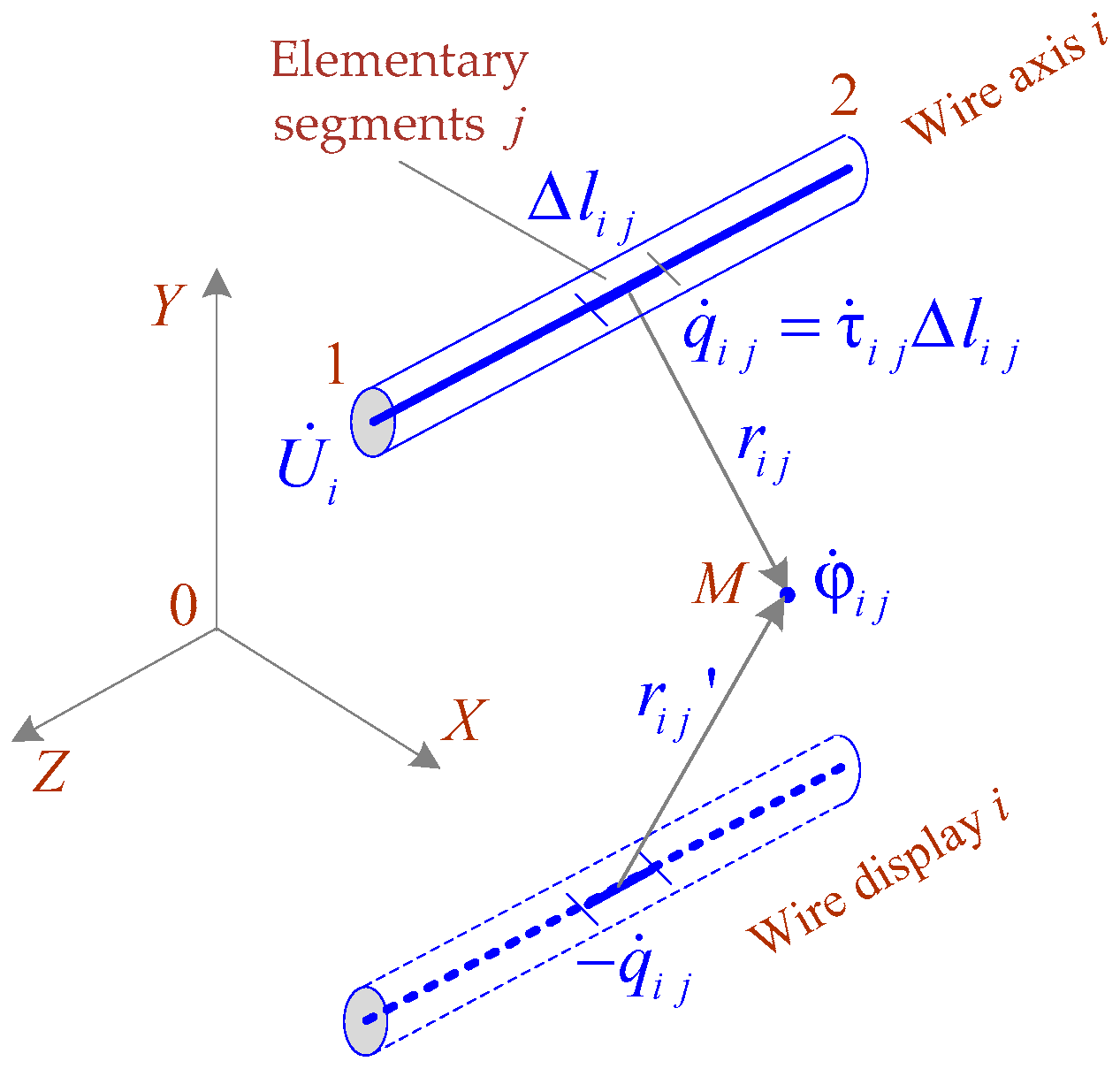
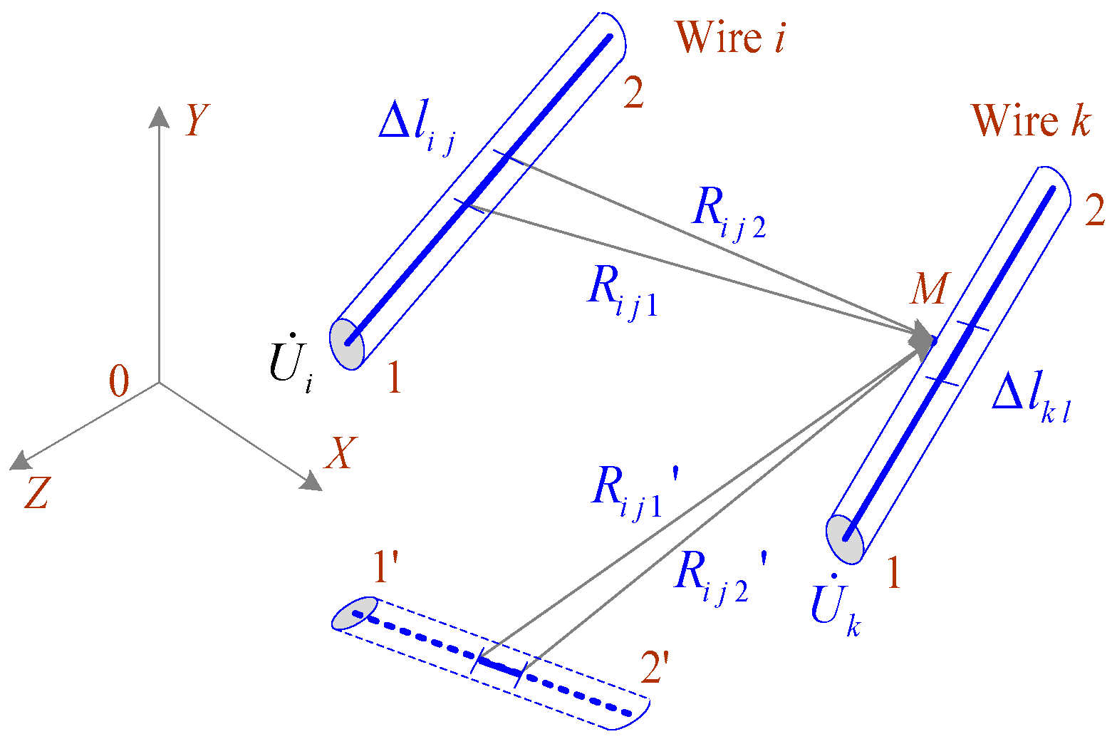
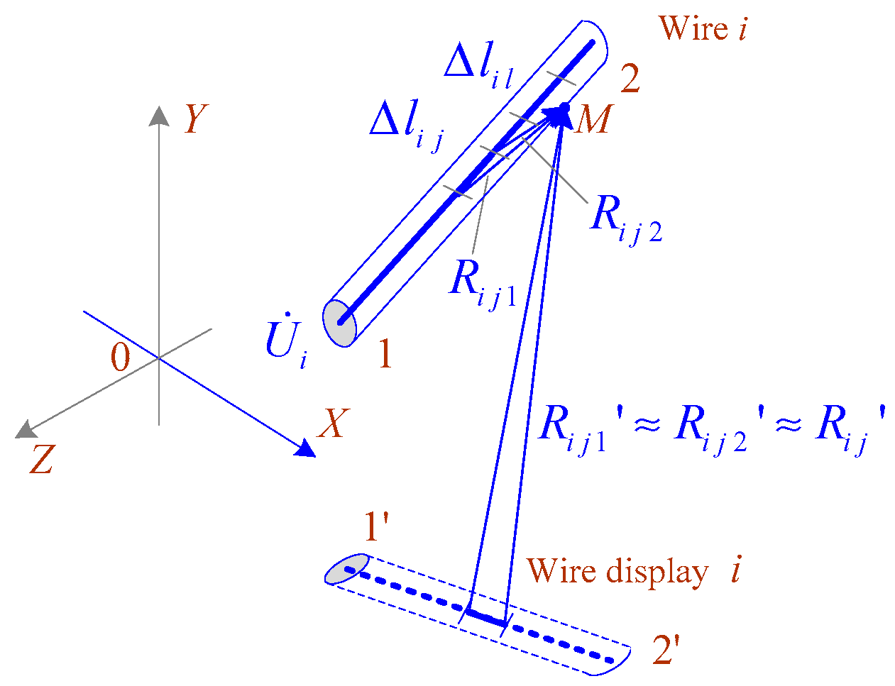
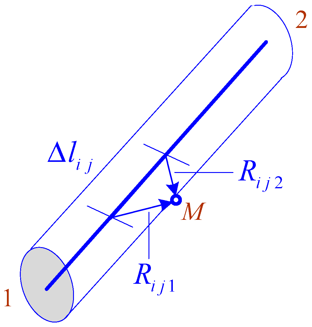
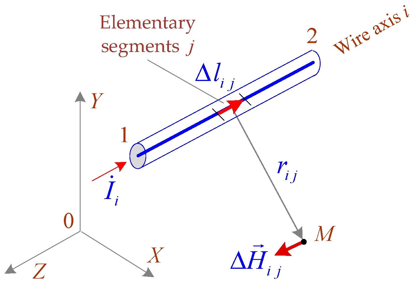
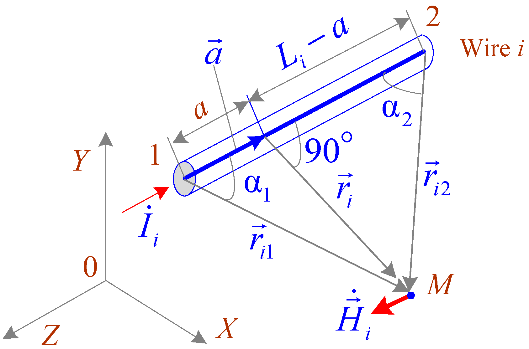
2. Modeling Technique

Computer technology for determining EMF [34] was intended to calculate the strengths of plane-parallel fields of objects whose cross-sectional dimensions are significantly smaller than their length. This approach did not allow analysis of the EMF of current-carrying parts of limited length, which include, for example, most components of substations. In addition, this method did not have the ability to take into account edge effects.

In the presence of limited length conductors, the EMF becomes three-dimensional, and the modeling becomes significantly more complicated. The method proposed in [33] to resolve this issue is based on the following basic principles:

• The current-carrying parts are represented in the form of straight segments, which are located in space according to the design of the object; some components, in particular, cables and parts of grounding systems, may be buried. To use the equations of a quasi-stationary zone, the size of the set of objects should not exceed several hundred meters.
• The analyzed network may include power lines and traction networks, transformers, loads, and sets of short conductors, which are modeled in the same way as power transmission line wires for calculation of operating parameters. The resistances of the wires are small; hence, this approach does not distort the network operating parameters. In addition, short-length grounded conductors can be used, specifically to model supports of power transmission lines and traction networks, substation portals, lightning rods, and others.
• The potentials and currents of short wires are determined by calculating the operating parameters in phase coordinates [32].
• The electric field is determined by the method of equivalent charges; the Bio-Savart formulas are used to calculate the magnetic field induction.
• Plain X0Z of the Cartesian coordinate system corresponds to the surface of the earth, the X axis is perpendicular to the railway route, and the Y axis is directed vertically upward.

The coordinate system and the short wire (SW) are shown in Figure 1. In the general case, the presence of N_w SW is assumed. Currents ${\dot{I}}_{ij}$ of normal or emergency modes can flow through them. Some grounded objects have ${\dot{I}}_{ij}=0$. Each SW i of length $L_i$ is represented as n_i elementary segments (ES) with lengths $∆l_i=L_i/n_i$ (Figure 2). For a more precise indication of the location of ES on wire i, the notation $∆l_{i j}$ can be used. The numbering of ES starts with one.

The potential created by wire i at observation point M with coordinates (x, y, z) is defined as follows [33]:

$${\dot{\mathrm{\phi }}}_i={\displaystyle \frac{1}{4{\mathrm{\pi }\mathrm{\epsilon }}_0}}{\displaystyle \underset{0}{\overset{L_i}{\int }}\left[\left(\frac{1}{r}-\frac{1}{r^{\prime }}\right){\dot{\mathrm{\tau }}}_{i}d{l}_{i j}\right]}\approx {\displaystyle \frac{1}{4{\mathrm{\pi }\mathrm{\epsilon }}_0}}{\displaystyle \sum _{j=1}^{n_i}\left(\frac{1}{r_{i j}}-\frac{1}{{r_{i j}}^{\prime }}\right){\dot{q}}_{i j}},$$

(1)

where $r_{i j}$—distance from M to the midpoint of the segment $∆l_{i j}$; ${r_{i j}}^{\prime }$—similar parameter for mirror image of ES; ${\dot{q}}_{i j}={\dot{\mathrm{\tau }}}_{i j}∆ l_{i j}$—charge of ES j of wire i; and $n_i$—number of ES.

Distances $r_{i j}$ and ${r_{i j}}^{\prime }$ are calculated using the coordinates of the beginning $x_{i1}, y_{i1}, z_{i1}$ and end $x_{i2}, y_{i2}, z_{i2}$ of the short wire

$$r_{i j}=\sqrt{{[x-x_{i1}-(j-0.5)∆x_i]}^2+{[y-y_{i1}-(j-0.5)∆y_i]}^2+{[z-z_{i1}-(j-0.5)∆z_i]}^2};$$

$${r_{i j}}^{\prime }=\sqrt{{[x-x_{i1}-(j-0.5)∆x_i]}^2+{[y+{y_{i1}}^{\prime }+(j-0.5)∆y_i]}^2+{[z-z_{i1}-(j-0.5)∆z_i]}^2};$$

where $∆x_i=(x_{i2}-x_{i1})/n_i$; $∆y_i=(y_{i2}-y_{i1})/n_i$; $∆z_i=(z_{i2}-z_{i1})/n_i$.

The potential at point M is calculated using the expression

$${\dot{\mathrm{\phi }}}_{i j}={\displaystyle \frac{{\dot{\mathrm{\tau }}}_{i j}}{4{\mathrm{\pi }\mathrm{\epsilon }}_0}}\ln \frac{\left(r_{i j 1}+r_{i j 2}+∆l_i\right)\left({r_{i j 1}}^{\prime }+{r_{i j 2}}^{\prime }-∆l_i\right)}{\left(r_{i j 1}+r_{i j 2}-∆l_i\right)\left({r_{i j 1}}^{\prime }+{r_{i j 2}}^{\prime }+∆l_i\right)},$$

(2)

where $r_{i j 1}$, $r_{i j 2}$, ${r_{i j 1}}^{\prime }$, and ${r_{i j 2}}^{\prime }$ are the distances to point M, corresponding to the beginning and end of the ES j and its reflection:

$$r_{i j 1}=\sqrt{{[x-x_{i1}-(j-1)∆x_i]}^2+{[y-y_{i1}-(j-1)∆y_i]}^2+{[z-z_{i1}-(j-1)∆z_i]}^2};$$

$$r_{i j 2}=\sqrt{{[x-x_{i1}-j ∆x_i]}^2+{[y-y_{i1}-j ∆y_i]}^2+{[z-z_{i1}-j ∆z_i]}^2};$$

$${r_{i j 1}}^{\prime }=\sqrt{{[x-x_{i1}-(j-1)∆x_i]}^2+{[y+y_{i1}+(j-1)∆y_i]}^2+{[z-z_{i1}-(j-1)∆z_i]}^2};$$

$${r_{i j 2}}^{\prime }=\sqrt{{[x-x_{i1}-j ∆x_i]}^2+{[y+y_{i1}+j ∆y_i]}^2+{[z-z_{i1}-j ∆z_i]}^2}.$$

${\dot{\mathrm{\tau }}}_{i j}$ can be determined from the solution of the following system:

$$\left\{\begin{array}{l}{\mathrm{\alpha }}_{11}{\dot{\mathrm{\tau }}}_1+\dots +{\mathrm{\alpha }}_{1,n1}{\dot{\mathrm{\tau }}}_{n1}+{\mathrm{\alpha }}_{1,n1+1}{\dot{\mathrm{\tau }}}_{n1+1}+\dots +{\mathrm{\alpha }}_{1,Ns}{\dot{\mathrm{\tau }}}_{Ns}=4{\mathrm{\pi }\mathrm{\epsilon }}_0{\dot{\mathrm{\varphi }}}_1;\\ {\mathrm{\alpha }}_{21}{\dot{\mathrm{\tau }}}_1+\dots +{\mathrm{\alpha }}_{2,n1}{\dot{\mathrm{\tau }}}_{n1}+{\mathrm{\alpha }}_{2,n1+1}{\dot{\mathrm{\tau }}}_{n1+1}+\dots +{\mathrm{\alpha }}_{2,Ns}{\dot{\mathrm{\tau }}}_{Ns}=4{\mathrm{\pi }\mathrm{\epsilon }}_0{\dot{\mathrm{\varphi }}}_1;\\ ...................................................\\ {\mathrm{\alpha }}_{k,1}{\dot{\mathrm{\tau }}}_1+\dots +{\mathrm{\alpha }}_{k,n1}{\dot{\mathrm{\tau }}}_{n1}+{\mathrm{\alpha }}_{k,n1+1}{\dot{\mathrm{\tau }}}_{n1+1}+\dots +{\mathrm{\alpha }}_{k,Ns}{\dot{\mathrm{\tau }}}_{Ns}=4{\mathrm{\pi }\mathrm{\epsilon }}_0{\dot{\mathrm{\varphi }}}_k;\\ ...................................................\\ {\mathrm{\alpha }}_{Ns,1}{\dot{\mathrm{\tau }}}_1+\dots +{\mathrm{\alpha }}_{Ns,n1}{\dot{\mathrm{\tau }}}_{n1}+{\mathrm{\alpha }}_{Ns,n1+1}{\dot{\mathrm{\tau }}}_{n1+1}+\dots +{\mathrm{\alpha }}_{Ns,Ns}{\dot{\mathrm{\tau }}}_{Ns}=4{\mathrm{\pi }\mathrm{\epsilon }}_0{\dot{\mathrm{\varphi }}}_{Ns},\end{array}\right.$$

(3)

where $N_S={\displaystyle \sum _{i=1}^{Nw}{n}_i}$.

The following expressions are used to calculate potential coefficients ${\mathrm{\alpha }}_{ij}$:

$${\mathrm{\alpha }}_{i j}=\ln {\displaystyle \frac{(R_{i j 1}+R_{i j 2}+∆l_i)({R_{i j 1}}^{\prime }+{R_{i j 2}}^{\prime }-∆l_i)}{(R_{i j 1}+R_{i j 2}-∆l_i)({R_{i j 1}}^{\prime }+{R_{i j 2}}^{\prime }+∆l_i)}},$$

(4)

in this case, ${\mathrm{\alpha }}_{i j}\ne {\mathrm{\alpha }}_{j i}$.

If ES j and l are located at different SWs with numbers i and k, then the distances are calculated as follows:

$$R_{i j 1}=\sqrt{{(x_{kl1}-x_{ij1})}^2+{(y_{kl1}-y_{ij1})}^2+{(z_{kl1}-z_{ij1})}^2};$$

$$x_{k l1}-x_{i j1}=x_{k 1}+(l-0.5)∆x_k-x_{i1}-(j-1)∆x_i;$$

$$y_{k l1}-y_{i j1}=y_{k 1}+(l-0.5)∆y_k-y_{i1}-(j-1)∆y_i;$$

$$z_{k l1}-z_{i j1}=z_{k 1}+(l-0.5)∆z_k-z_{i1}-(j-1)∆z_i;$$

$$R_{ij 2}=\sqrt{{(x_{k l2}-x_{i j2})}^2+{(y_{k l2}-y_{i j2})}^2+{(z_{k l2}-z_{i j2})}^2};$$

$$x_{k l2}-x_{i j2}=x_{k 1}+(l-0.5)∆x_k-x_{i1}-j ∆x_i;$$

$$y_{k l2}-y_{i j2}=y_{k 1}+(l-0.5) ∆y_k-y_{i1}-j ∆y_i;$$

$$z_{k l2}-z_{i j2}=z_{k 1}+(l-0.5) ∆z_k-z_{i1}-j ∆z_i;$$

$${R_{i j 1}}^{\prime }\approx {R_{i j 2}}^{\prime }\approx \sqrt{{(x_{k l1}-{x_{i j1}}^{\prime })}^2+{(y_{k l1}-{y_{i j1}}^{\prime })}^2+{(z_{k l1}-{z_{i j1}}^{\prime })}^2};$$

$$x_{k l1}-{x_{i j1}}^{\prime }=x_{k 1}+(l-0.5) ∆x_k-x_{i1}-(j-0.5) ∆x_i;$$

$$y_{k l1}-{y_{i j1}}^{\prime }=y_{k 1}+(l-0.5) ∆y_k+y_{i1}+(j-0.5) ∆y_i;$$

$$z_{k l1}-{z_{i j1}}^{\prime }=z_{k 1}+(l-0.5) ∆z_k-z_{i1}-(j-0.5) ∆z_i.$$

When the ES is located on one SW, $j\ne l$, and the ES index, near which the point M is located (Figure 3), is designated by the symbol l, then we can write

$$R_{i j 1}\approx \left|(l-j+0.5)\right| ∆l_i; R_{i j 2}\approx \left|(l-j-0.5)\right| ∆l_i.$$

(5)

In this case, the contribution of the reflection charges of the SW can be determined as follows:

$${\mathrm{\alpha }}_{i j}=\ln {\displaystyle \frac{R_{i j 1}+R_{i j 2}+∆l_i}{R_{i j 1}+R_{i j 2}-∆l_i}}-{\displaystyle \frac{∆l_i}{{R_{i j}}^{\prime }}},$$

(6)

$${R_{ij}}^{\prime }\approx \sqrt{{[(l-j)∆x_i]}^2+{[2y_{i1}+2(l-j)∆y_i]}^2+{[(l-j)∆z_i]}^2}.$$

(7)

If $j=l$ (Figure 4), then (6) is applied with the calculation of distances within the ES according to the following expression:

$$R_{i i 1}=R_{i i 2}=\sqrt{{(0.5∆l_i)}^2+{R_i}^2},$$

(8)

where $R_i$ is radius of the SW i.

Based on the found ${\dot{\mathrm{\tau }}}_{i j}$, the components of the stress at point M are calculated using the formulas ${\dot{q}}_{i j}={\dot{\mathrm{\tau }}}_{i j}∆l_i$:

$$\dot{\overrightarrow{E}}={\displaystyle \frac{1}{4{\mathrm{\pi }\mathrm{\epsilon }}_0}}{\displaystyle \sum _{i=1}^{Nw}{\displaystyle \sum _{j=1}^{n_i}{\dot{q}}_{i j}\left(\frac{{\overrightarrow{e}}_{\mathrm{r}}}{{r_{i j}}^2}-\frac{{{\overrightarrow{e}}_{\mathrm{r}}}^{\prime }}{{r_{i j}}^{\prime 2}}\right)}},$$

(9)

where

$$r_{i j}=\sqrt{{[x-x_{i 1}-(j-0.5)∆x_i]}^2+{[y-y_{i1}-(j-0.5)∆y_i]}^2+{[z-z_{i 1}-(j-0.5)∆z_i]}^2};$$

$${r_{i j}}^{\prime }=\sqrt{{[x-x_{i1}-(j-0.5)∆x_i]}^2+{[y+y_{i1}+(j-0.5)∆y_i]}^2+{[z-z_{i 1}-(j-0.5)∆z_i]}^2};$$

$${\overrightarrow{e}}_{\mathrm{r}}={\displaystyle \frac{x-x_{i1}-(j-0.5)∆x_i}{r_{i j}}}{\overrightarrow{e}}_{\mathrm{x}}+{\displaystyle \frac{y-y_{i1}-(j-0.5)∆y_i}{r_{i j}}}{\overrightarrow{e}}_{\mathrm{y}}+{\displaystyle \frac{z-z_{i1}-(j-0.5)∆z_i}{r_{i j}}}{\overrightarrow{e}}_{\mathrm{z}};$$

$${{\overrightarrow{e}}_{\mathrm{r}}}^{\prime }={\displaystyle \frac{x-x_{i1}-(j-0.5)∆x_i}{{r_{i j}}^{\prime }}}{\overrightarrow{e}}_{\mathrm{x}}+{\displaystyle \frac{y+y_{i1}+(j-0.5)∆y_i}{{r_{i j}}^{\prime }}}{\overrightarrow{e}}_{\mathrm{y}}+{\displaystyle \frac{z-z_{i1}-(j-0.5)∆z_i}{{r_{i j}}^{\prime }}}{\overrightarrow{e}}_{\mathrm{z}},$$

where ${\overrightarrow{e}}_{\mathrm{r}}$, ${{\overrightarrow{e}}_{\mathrm{r}}}^{\prime }$ are direction vectors from the middle of the ES and from its mirror image to M; ${\overrightarrow{e}}_{\mathrm{x}}$, ${\overrightarrow{e}}_{\mathrm{y}}$, ${\overrightarrow{e}}_{\mathrm{z}}$ are orts.

Calculations of the magnetic field strength of the SW system can be carried out using the Biot–Savart formulas after determining the mode

$$∆ {\dot{\overrightarrow{H}}}_{i j}={\displaystyle \frac{{\dot{I}}_i}{4\mathrm{\pi } {r_{i j}}^3}}(∆ {\overrightarrow{l}}_{i j}\times {\overrightarrow{r}}_{i j}),$$

(10)

where $∆{\overrightarrow{H}}_{i j}$ is the addition from the EW with number j of the wire i (Figure 5); ${\overrightarrow{r}}_{i j}$ is the vector from the element $∆ {\overrightarrow{l}}_{i j}$ to point M.

The vector product has the following projections onto the coordinate axes:

$$∆ {\overrightarrow{l}}_{i j}={\displaystyle \frac{1}{n_i}}\left[(x_{i2}-x_{i1}) {\overrightarrow{e}}_{\mathrm{x}}+(y_{i2}-y_{i1}) {\overrightarrow{e}}_{\mathrm{y}}+(z_{i2}-z_{i1}) {\overrightarrow{e}}_{\mathrm{z}}\right];$$

$$r_{i j}=\sqrt{{[x_i+(j-0.5)∆x_i]}^2+{[y_i+(j-0.5)∆y_i]}^2+{[z_i+(j-0.5)∆z_i]}^2};$$

$${\overrightarrow{r}}_{i j}={\displaystyle \frac{1}{r_{i j}}}(x_{i j} {\overrightarrow{e}}_{\mathrm{x}}+y_{i j} {\overrightarrow{e}}_{\mathrm{y}}+z_{i j} {\overrightarrow{e}}_{\mathrm{z}}); x_i=x_{i1}-x; y_i=y_{i1}-y; z_i=z_{i1}-z;$$

$$x_{i j}=x_i+(j-0.5)∆x_i; y_{i j}=y_i+(j-0.5)∆y_i; z_{i j}=z_i+(j-0.5)∆z_i;$$

$$∆x_i =(x_{i2}-x_{i1})/n_i; ∆y_i =(y_{i2}-y_{i1})/n_i; ∆z_i =(z_{i2}-z_{i1})/n_i;$$

$$∆{\dot{H}}_{i j X}={\displaystyle \frac{{\dot{I}}_i}{4\mathrm{\pi } n_i{r_{i j}}^3}}\left[(y_{i2}-y_{i1}) {\displaystyle \frac{z_{i j}}{r_{i j}}}-(z_{i 2}-z_{i 1}) {\displaystyle \frac{y_{i j}}{r_{i j}}}\right];$$

(11)

$$∆{\dot{H}}_{i j Y}={\displaystyle \frac{{\dot{I}}_i}{4\mathrm{\pi } n_i{r_{i j}}^3}}\left[(z_{i2}-z_{i1}) {\displaystyle \frac{x_{i j}}{r_{i j}}}-(x_{i 2}-x_{i 1}) {\displaystyle \frac{z_{i j}}{r_{i j}}}\right];$$

(12)

$$∆{\dot{H}}_{i j Z}={\displaystyle \frac{{\dot{I}}_i}{4\mathrm{\pi } n_i{r_{i j}}^3}}\left[(x_{i 2}-x_{i 1}) {\displaystyle \frac{y_{i j}}{r_{i j}}}-(y_{i 2}-y_{i 1}) {\displaystyle \frac{x_{i j}}{r_{i j}}}\right];$$

(13)

$${\dot{H}}_X={\displaystyle \sum _{i=1}^{N1}{\displaystyle \sum _{j=1}^{n_i}∆{\dot{H}}_{i j X}}}; {\dot{H}}_Y={\displaystyle \sum _{i=1}^{N1}{\displaystyle \sum _{j=1}^{n_i}∆{\dot{H}}_{i j Y}}}; {\dot{H}}_Z={\displaystyle \sum _{i=1}^{N1}{\displaystyle \sum _{j=1}^{n_i}∆{\dot{H}}_{i j Z}}}.$$

(14)

The direction $∆ {\overrightarrow{l}}_{i j}$ is determined by the location of the start points 1 and end points 2 of the ES.

The magnetic field strength of the SW can be determined using the following expression (Figure 6):

$${\dot{H}}_i={\displaystyle \frac{{\dot{I}}_i}{4\mathrm{\pi } r_i}}(\cos {\mathrm{\alpha }}_1+\cos {\mathrm{\alpha }}_2),$$

$$r_i=\sqrt{{(x-x_a)}^2+{(y-y_a)}^2+{(z-z_a)}^2}; r_{i1}=\sqrt{{(x-x_1)}^2+{(y-y_1)}^2+{(z-z_1)}^2};$$

$$r_{i 2}=\sqrt{{(x-x_2)}^2+{(y-y_2)}^2+{(z-z_2)}^2}; a=\sqrt{{(x_a-x_1)}^2+{(y_a-y_1)}^2+{(z_a-z_1)}^2}.$$

Angles ${\mathrm{\alpha }}_1$ and ${\mathrm{\alpha }}_2$ are calculated using scalar multiplications:

$$\cos {\mathrm{\alpha }}_1={\displaystyle \frac{{\overrightarrow{r}}_{12}·{\overrightarrow{r}}_{i1}}{r_{12}·r_{i1}}}; \cos {\mathrm{\alpha }}_2=-{\displaystyle \frac{{\overrightarrow{r}}_{12}·{\overrightarrow{r}}_{i2}}{r_{12}·r_{i2}}};$$

$${\overrightarrow{r}}_{12}·{\overrightarrow{r}}_{i1}=(x_2-x_1) (x-x_1)+(y_2-y_1) (y-y_1)+(z_2-z_1) (z-z_1);$$

$${\overrightarrow{r}}_{12}·{\overrightarrow{r}}_{i 2}=(x_2-x_1) (x-x_2)+(y_2-y_1) (y-y_2)+(z_2-z_1) (z-z_2).$$

The coordinates of the beginning $(x_a, y_a, z_a)$ of the perpendicular $r_i$ are determined as follows

$$\left\{\begin{array}{l}{y}_{21}(x_a-x_1)=x_{21}(y_a-y_1);\\ z_{21}(y_a-y_1)=y_{21}(z_a-z_1);\\ x_{21}(x_a-x)+y_{21}(y_a-y)+z_{21}(z_a-z)=0,\end{array}\right.$$

where $x_{21}=x_2-x_1$; $y_{21}=y_2-y_1$; $z_{21}=z_2-z_1$.

The coordinates of the division point of the SW by the perpendicular drawn from M, at $x_{21}\ne 0$, are equal to

$$y_a=y_1+{\displaystyle \frac{y_{21}}{x_{21}}}(x_a-x_1); z_a=z_1+{\displaystyle \frac{z_{21}}{y_{21}}}(y_a-y_1)=z_1+{\displaystyle \frac{z_{21}}{x_{21}}}(x_a-x_1);$$

$$x_{21}(x_a-x)+y_{21}\left[y_1+{\displaystyle \frac{y_{21}}{x_{21}}}(x_a-x_1)-y\right]+z_{21}\left[z_1+{\displaystyle \frac{z_{21}}{x_{21}}}(x_a-x_1)-z\right]=0;$$

$$x_{21}{x}_a-x_{21}x+y_{21}{y}_1+{\displaystyle \frac{{y_{21}}^2}{x_{21}}}(x_a-x_1)-y_{21}y+z_{21}{z}_1+{\displaystyle \frac{{z_{21}}^2}{x_{21}}}(x_a-x_1)-z_{21}z=0;$$

$$x_a={\displaystyle \frac{x_{21}x-y_{21}(y_1-y)-z_{21}(z_1-z)+x_1({y_{21}}^2+{z_{21}}^2)/x_{21}}{x_{21}+({y_{21}}^2+{z_{21}}^2)/x_{21}}}.$$

The following options are possible:

1. $x_{21}=0$; $y_{21}\ne 0$; $z_{21}\ne 0$.

$$x_a=x_1; y_a={\displaystyle \frac{y_{21}{z}_{21}(z-z_1)+{y_{21}}^{2}y+{z_{21}}^2{y}_1}{{y_{21}}^2+{z_{21}}^2}};z_a=z-{\displaystyle \frac{y_{21}}{z_{21}}}(y_a-y).$$

2. $x_{21}=0$; $y_{21}\ne 0$; $z_{21}=0$.

$$x_a=x_1; y_a=y;z_a=z_1.$$

3. $x_{21}=0$; $y_{21}=0$; $z_{21}\ne 0$.

$$x_a=x_1; y_a=y_1; z_a=z.$$

The direction ${\overrightarrow{\dot{H}}}_i$ is determined by vector multiplication, where

${\overrightarrow{r}}_{12}=(x_2-x_1) \overrightarrow{i}+(y_2-y_1) \overrightarrow{j}+(z_2-z_1) \overrightarrow{k}$ is the wire axis vector.

This can be written as

$$c_x={\displaystyle \frac{{({\overrightarrow{r}}_{12}\times {\overrightarrow{r}}_{i1})}_x}{\left|{\overrightarrow{r}}_{12}\times {\overrightarrow{r}}_{i1}\right|}}={\displaystyle \frac{c_{m x}}{c_m}}; c_y={\displaystyle \frac{{({\overrightarrow{r}}_{12}\times {\overrightarrow{r}}_{i1})}_y}{\left|{\overrightarrow{r}}_{12}\times {\overrightarrow{r}}_{i1}\right|}}={\displaystyle \frac{c_{my}}{c_m}}; c_z={\displaystyle \frac{{({\overrightarrow{r}}_{12}\times {\overrightarrow{r}}_{i1})}_z}{\left|{\overrightarrow{r}}_{12}\times {\overrightarrow{r}}_{i1}\right|}}={\displaystyle \frac{c_{mz}}{c_m}};$$

$$c_m=\sqrt{{c_{mx}}^2+{c_{my}}^2+{c_{mz}}^2};c_{mx}=(y_2-y_1) (z-z_1)-(z_2-z_1) (y-y_1);$$

$$c_{my}=(z_2-z_1) (x-x_1)-(x_2-x_1) (z-z_1);c_{mz}=(x_2-x_1) (y-y_1)-(y_2-y_1) (x-x_1);$$

$${\dot{H}}_{ix}={\dot{H}}_i c_x; {\dot{H}}_{iy}={\dot{H}}_i c_y; {\dot{H}}_{iz}={\dot{H}}_i c_z;$$

(15)

$${\dot{H}}_x={\displaystyle \sum _{i=1}^{N1} {\dot{H}}_{i x}}; {\dot{H}}_y={\displaystyle \sum _{i=1}^{N1}{\dot{H}}_{i y}};{\dot{H}}_z={\displaystyle \sum _{i=1}^{N1}{\dot{H}}_{i z}}.$$

(16)

After calculating the intensities using Formulas (9) and (17), we can find the projections on the coordinate axes. For example, for the electric field

$$\overrightarrow{E}(t)=E_{m x}\sin (\mathrm{\omega } t+{\mathrm{\psi }}_x){\overrightarrow{e}}_{\mathrm{x}}+E_{m y}\sin (\mathrm{\omega } t+{\mathrm{\psi }}_x) {\overrightarrow{e}}_{\mathrm{y}}+E_{m z}\sin (\mathrm{\omega } t+{\mathrm{\psi }}_x) {\overrightarrow{e}}_{\mathrm{z}},$$

or

$$E_i(t)=E_{m i}\sin (\mathrm{\omega } t+{\mathrm{\psi }}_i), i=x, y, z.$$

The square of the instantaneous value is equal to

$$E^2(t)={\displaystyle \sum _{i=1}^3{[E_{m i}\sin (\mathrm{\omega } t+{\mathrm{\psi }}_i)]}^2}={\displaystyle \frac{1}{2}}{\displaystyle \sum _{i=1}^3{E_{m i}}^2[1-\cos (2\mathrm{\omega } t+2{\mathrm{\psi }}_i)]};$$

$$E^2(t)={\displaystyle \frac{1}{2}}{\displaystyle \sum _{i=1}^3{E_{m i}}^2}+{\displaystyle \frac{1}{2}}\sin 2\mathrm{\omega } t{\displaystyle \sum _{i=1}^3{E_{m i}}^2\sin 2{\mathrm{\psi }}_i}-{\displaystyle \frac{1}{2}}\cos 2\mathrm{\omega } t{\displaystyle \sum _{i=1}^3{E_{m i}}^2\cos 2{\mathrm{\psi }}_i}.$$

The extremes $E^2(t)$ are determined by the zeros of the derivative

The formulas for calculating the electric field strengths are obtained on the basis of the equivalent charge method, and the expressions for the magnetic field are derived using the Biot–Savart approach with the summation of the complex values of the field strengths of elementary segments and the superposition of the fields of all wires.

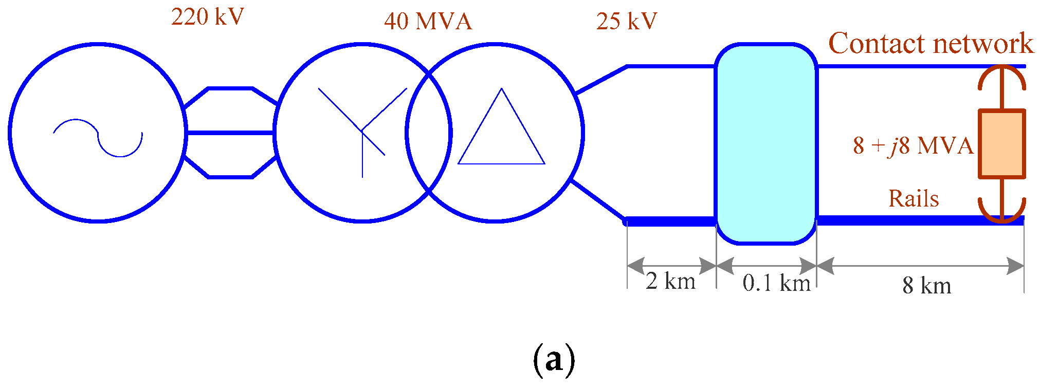
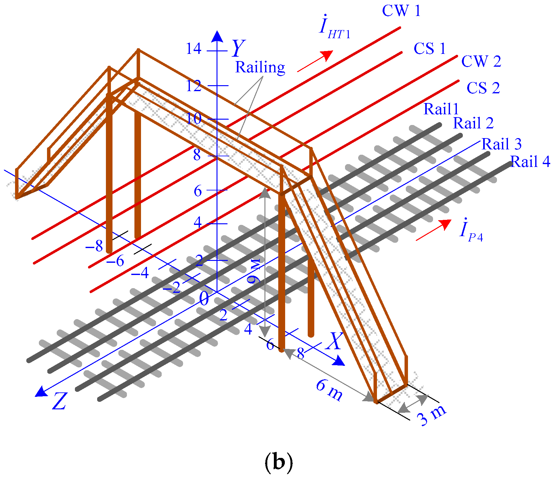
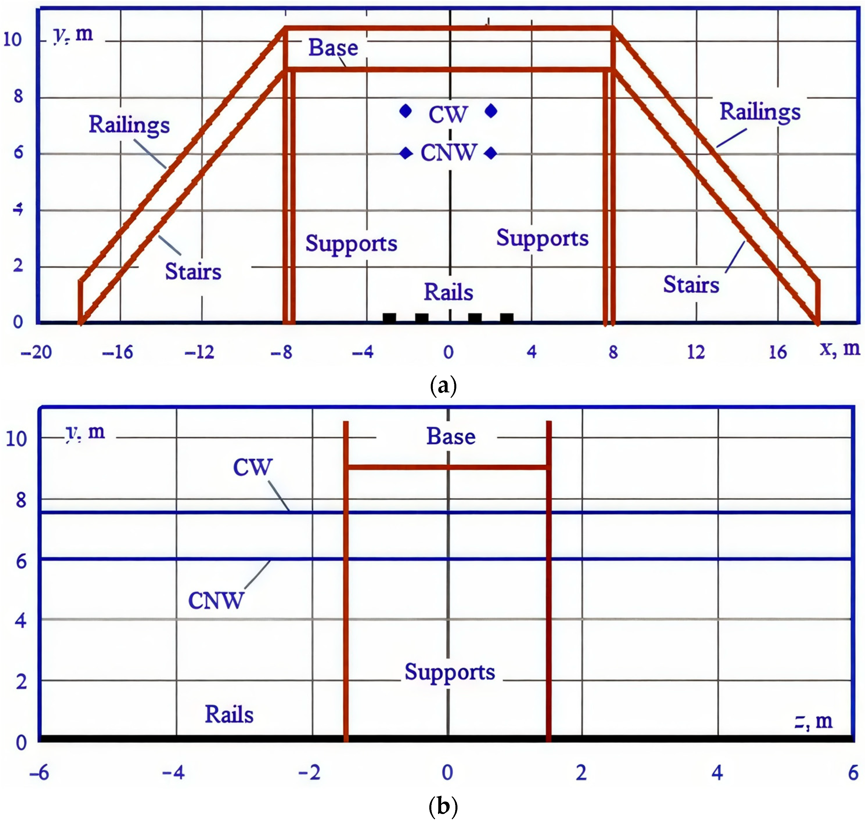
3. Model Description

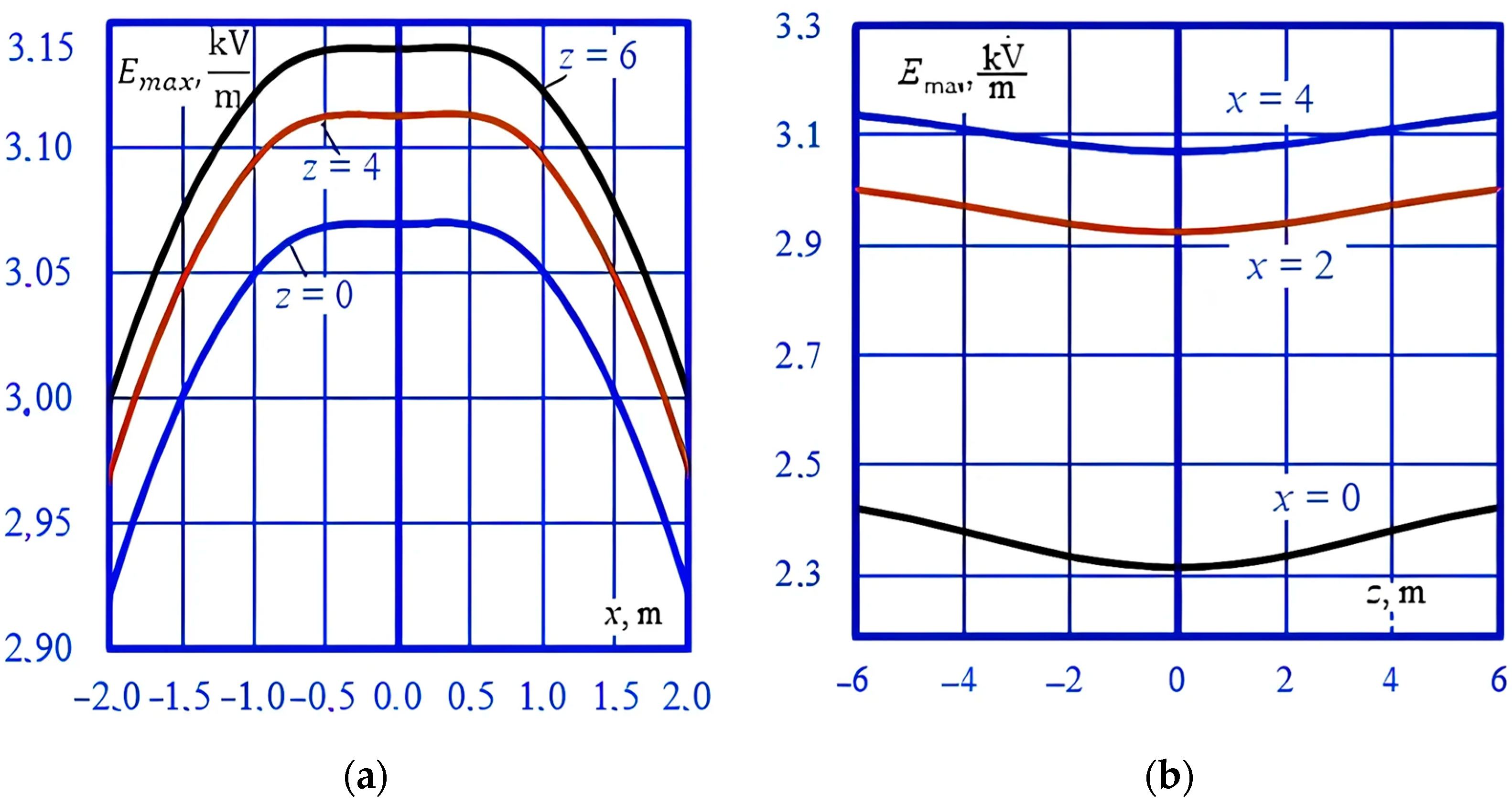
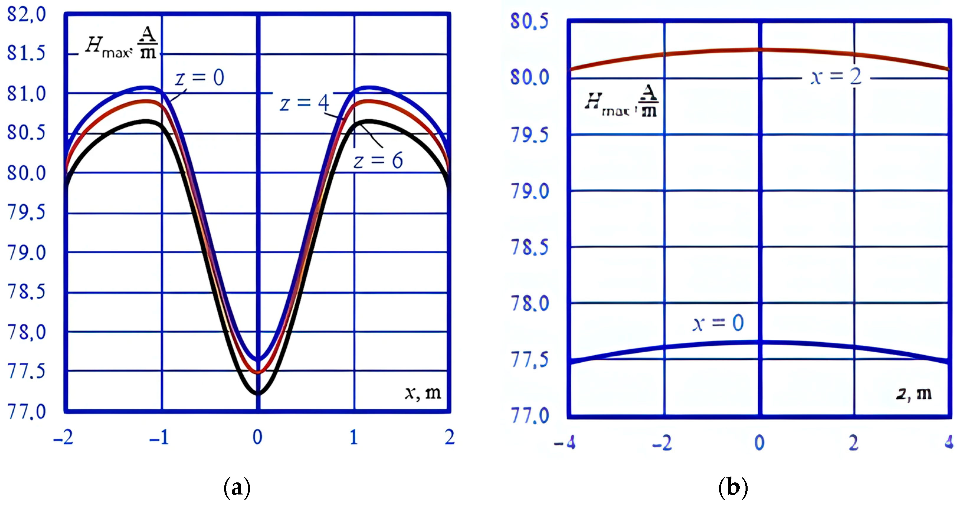
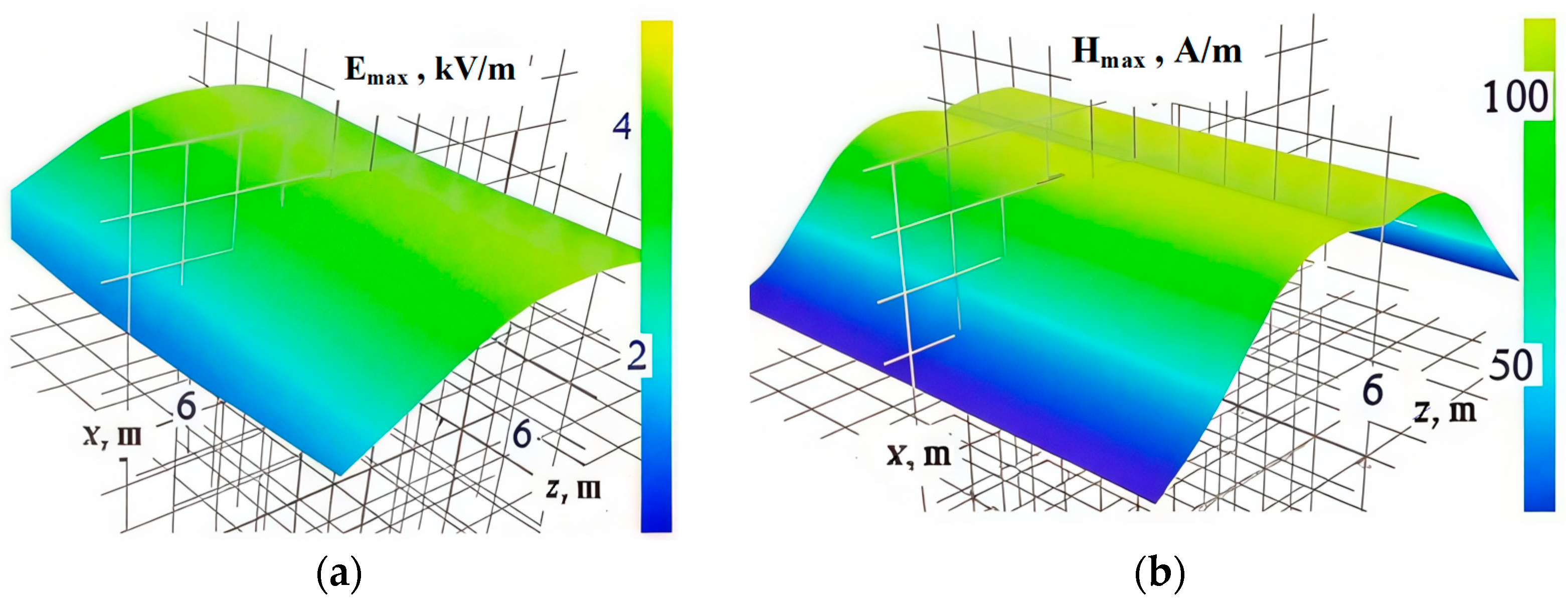
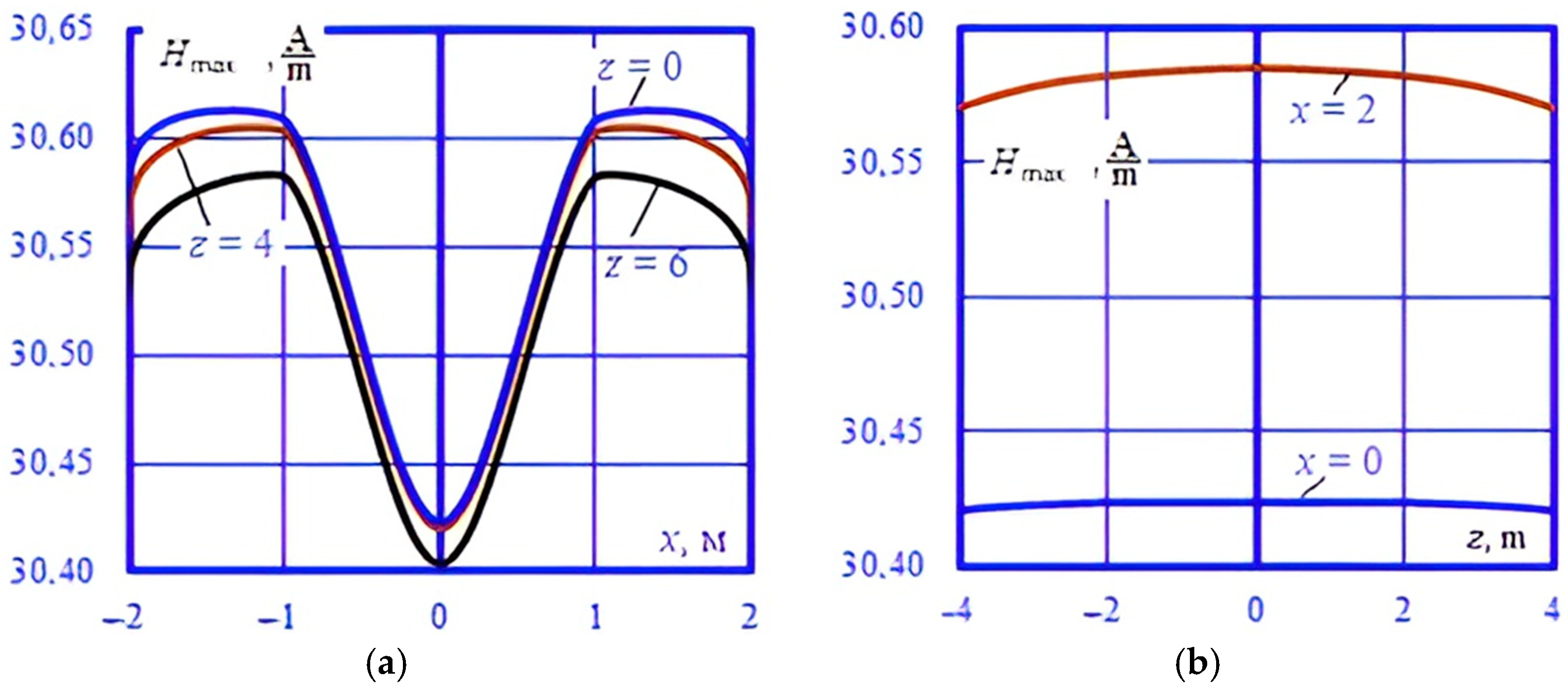
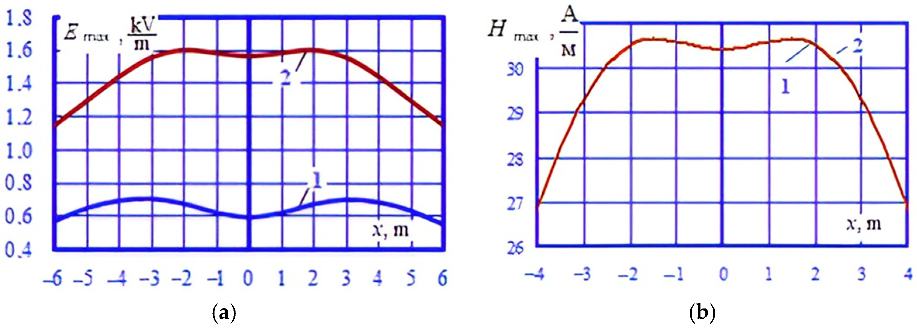
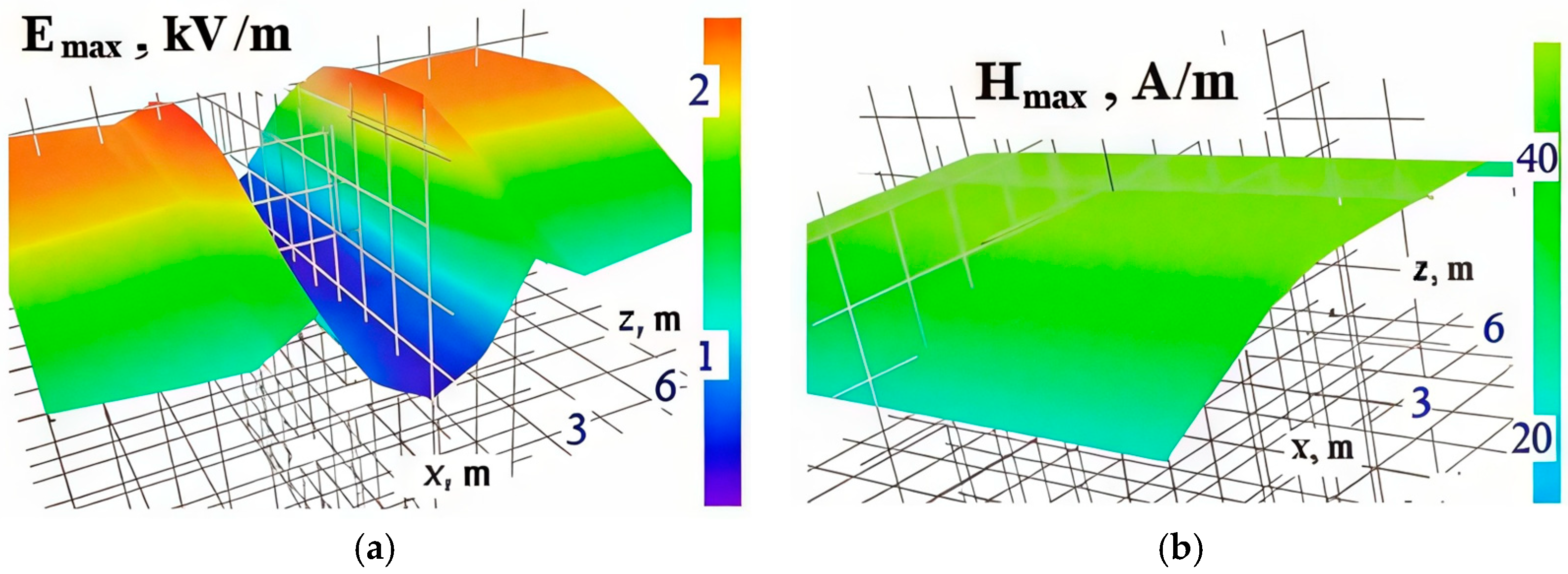
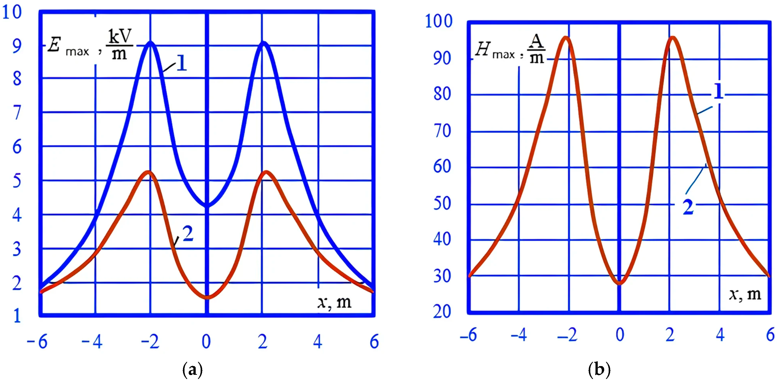
The modeled network includes a section of a double-track 25 kV AC railway with the following components: an equivalent generator of the power supply system, a traction substation with a 40 MVA transformer, a cantilever section of a 25 kV traction network 10 km long with a catenary suspension made of PBSM-95+MF-100 wires (Manufacturers of PBSM-95 are ZMI-profit LLC, and MF-100 cable is Volzhsky Kabel LLC, Russia). The model assumes an overpass three meters wide (at a distance of 2 km from the substation) with the base situated at a height of 9 m and takes into account railings. The layout of the objects is shown in Figure 7. The total current of the contact suspension of one track is 507 A.

The problems of determining EMF near an overpass are solved using the approach described in [33] and implemented in the Fazonord software of version 5.3.2.9-2023. A fragment of the calculation model diagram of the traction power supply system (TPSS), which was employed to calculate three-dimensional EMFs near the overpass, is shown in Figure 8. In order to implement the approach presented in [33], in addition to the power components described above, the models of the overpass and the short section of the traction network were formed using a set of short conductors. The length of the short section of the traction network was taken equal to 40 m. The ground conductivity was set at the level of 0.01 S/m. The details of the overpass are represented by sections of short wires, the location of which is shown in Figure 9, where different scales are assumed along the coordinate axes.

Representing the model of a traction network section with segments of short wires involves choosing its length L. The decrease in EMF strength at the edges of the model, caused by the limited length of the segments, should not affect the middle of the section; therefore, the value of L should not be too small. On the other hand, the constraints on the maximum size included in the calculation algorithm of line element ${\mathcal{l}}_0={\displaystyle \frac{L}{n}}$ force the selection of a sufficiently large number of its partitions n so that the distance s from the observation point to each segment satisfies the condition $s\ge 3{\mathcal{l}}_0$. Thus, the length of the traction network section is determined by a compromise between two conflicting requirements. In addition, obtaining EMF strengths in the middle of a short section of the traction network, which differs little from similar values of a long section, is evidence of the adequacy of the method proposed in [33].

4. Modeling Results

The optimal length of a short section of the traction network was selected by comparing the calculated EMF strengths at a height of 1.8 m for the middle of the short section and the beginning of the next two-kilometer section (nodes 38–45 according to the diagram in Figure 8a). The EMF for this section was determined in a plane-parallel formulation. In doing so, the elements modeling the overpass were removed from the diagram. As a result, the optimal length of the short section was chosen to be 40 m, which was divided into 200 line elements according to the methodology proposed in [33]. The results of EMF calculations for a point with coordinates x = 0 and z = 0 are given in

Table 1. Results of comparative EMF calculations for a height of 1.8 m.

Method	${\mathit{E}}_{\mathit{m}\mathit{a}\mathit{x}}, \frac{\mathbf{k}\mathbf{V}}{\mathbf{m}}$	${\mathit{H}}_{\mathit{m}\mathit{a}\mathit{x}}, \frac{\mathbf{A}}{\mathbf{m}}$
EMF of short wires	3.20 $\pm$ 0.04	77.67 $\pm$ 0.9
Plane-parallel EMF	3.26 $\pm$ 0.04	80.07 $\pm$ 0.9
Difference between the EMF of short wires and the plane-parallel field, %	−1.8	−3.0

.

The results of the EMF calculation for a height of 1.8 m are shown in Figure 10, Figure 11, Figure 12 and Figure 13 and Table 1.

As shown in Figure 10, Figure 11, Figure 12 and Figure 13, the amplitudes of the electric field strengths under the overpass at a height of 1.8 m decrease. On the axis of the structure (z = 0), the maximum decrease in the value of Emax reaches 20% due to the grounded structures. The relationship H_max= H_max(x) remains largely unchanged, even when considering the metal structure. Figure 14, Figure 15, Figure 16 and Figure 17 indicate similar dependences constructed for a height of 10.8 m, i.e., for a height of 1.8 m above the overpass.

As seen in Figure 14, Figure 15, Figure 16 and Figure 17, the presence of the overpass leads to a considerable reduction in the amplitudes of EMF strengths compared to its absence; at z = 0, the amplitude Emax decreases by 64% due to the shielding effect of the railings, while the curve H_max = H_max(x) remains virtually unchanged.

Figure 18 shows the results of modeling EMF at a height of 8 m, i.e., directly under the overpass. Both curves coincide for the magnetic field. This analysis is crucial because sensitive equipment, such as video surveillance cameras, may be affected by EMF when installed on the overpass.

Based on Figure 12, it can be concluded that in the presence of a grounded structure, the electric field strength at a height of 8 m increases by a maximum of 75%. The magnetic field remains unaffected by the overpass.

The described method of modeling EMF allows the following factors to be taken into account:

• The presence of rolling stock in the form of metal wagons and tanks under the overpass, which can have a noticeable effect on the distribution of electromagnetic field strengths in the space surrounding the overpass;
• Pipelines, reinforced concrete platforms, and metal fences, which also affect the nature of the distribution of EMF.

Based on the proposed method, it is possible to correctly account for the artificial structures of railways in the form of bridges with traffic above and below, galleries, and tunnels with a large number of metal structures that affect the values of field strengths. In addition to the normal mode considered in the article, the proposed method allows determining the EMF strengths in short-circuit modes of the contact suspension on the rails through the elements of the overpass structure.

5. Conclusions

The presented work is devoted to the study of the influence of conductive structures on the electromagnetic fields of the traction network.

In the presence of a metal structure, the EMF becomes three-dimensional and the modeling problem is significantly complicated. The methodology for solving it is based on the following main provisions:

• Current-carrying parts are represented as rectilinear segments that are located in space in accordance with the structure of the object; some elements, in particular grounding devices, can be located underground. To use the quasi-stationary zone equations, the dimensions of the set of objects should not exceed several hundred meters.
• The analyzed network can include power transmission lines and traction networks, transformers, loads, sets of short conductors, which are modeled in the same way as power transmission line wires for calculating the mode; due to the smallness of their resistance, this approach does not distort the network mode.
• The potentials and currents of short wires are determined by calculating the mode in phase coordinates.

The analysis of the results of modeling, performed on the basis of the Fazonord software package according to the technique described in the article, showed that the presence of a metal overpass significantly changes the nature of the distribution of EMF strengths in space, especially in the immediate vicinity of it. These changes must be taken into account when determining the influence of EMF on the operation of communication systems and electronic devices located near the railway infrastructure. Unlike the plane-parallel EMF created by the traction network in the spans between supports, the field in this situation becomes three-dimensional. The technology for determining the strengths presented in the article was based on the use of the concept of conductor segments of limited length, some of which can be located underground. To be able to apply the equations of the quasi-stationary zone, the dimensions of the set of objects formed by these conductors did not exceed several hundred meters. The technique is universal and can be used to model the EMF of almost any conductive structures. It can be used in the practice of designing and operating traction power supply systems when developing measures to improve electromagnetic safety conditions.

The described method of determining EMF is distinguished by the following features:

• Systematicity—consisting in the possibility of modeling electromagnetic fields taking into account the properties and characteristics of a complex STE and the power supply electric power system;
• Universality—ensuring the modeling of power transmission lines and traction networks of various designs;
• Adequacy to the external environment—achieved by taking into account the profile of the underlying surface, underground communications, metal structures, artificial structures of railway transport, such as galleries, bridges, and tunnels;
• Complexity—ensured by combining the calculations of the mode and the determination of EMF strengths.

References

1. Kosarev, A.B.; Kosarev, B.I. Fundamentals of Electromagnetic Safety for Power Supply Systems of Railway Transport; Intext: Moscow, Russia, 2008; 480p. [Google Scholar]
2. Suslov, K.; Kryukov, A.; Voronina, E.; Fesak, I. Modeling Power Flows and Electromagnetic Fields Induced by Compact Overhead Lines Feeding Traction Substations of Mainline Railroads. Appl. Sci. 2023, 13, 4249. [Google Scholar] [CrossRef]
3. Oancea, C.D.; Calin, F.; Golea, V. On the Electromagnetic Field in the Surrounding Area of Railway Equipment and Installations. In Proceedings of the 2019 International Conference on Electromechanical and Energy Systems (SIELMEN), Craiova, Romania, 9–11 October 2019; pp. 1–5. [Google Scholar] [CrossRef]
4. Zhang, L.; Zhu, Y.; Chen, S.; Zhang, D. Simulation and Analysis for Electromagnetic Environment of Traction Network. In Proceedings of the 2021 XXXIVth General Assembly and Scientific Symposium of the International Union of Radio Science (URSI GASS), Rome, Italy, 28 August–4 September 2021; pp. 1–4. [Google Scholar] [CrossRef]
5. Lu, N.; Zhu, F.; Yang, C.; Yang, Y.; Lu, H.; Wang, Z. The Research on Electromagnetic Emission of Traction Network With Short-Circuit Current Puls. IEEE Trans. Transp. Electrif. 2022, 8, 2029–2036. [Google Scholar] [CrossRef]
6. Zalesova, O.V. Estimation of Induced Voltage on the Dead Overhead Power Line caused by Electromagnetic Influence of the 25 kV AC Electric Railway System. In Proceedings of the 2019 International Multi-Conference on Industrial Engineering and Modern Technologies (FarEastCon), Vladivostok, Russia, 1–4 October 2019; pp. 1–4. [Google Scholar] [CrossRef]
7. Serdiuk, T.; Serdiuk, K.; Profatylov, V.; Adhena, H.H.; Thomas, D.; Greedy, S. Analysis of Electrified Systems and Electromagnetic Interference on the Railways. IEEE Lett. Electromagn. Compat. Pract. Appl. 2023, 5, 3. [Google Scholar] [CrossRef]
8. Serdiuk, T.; Feliziani, M.; Serdiuk, K. About Electromagnetic Compatibility of Track Circuits with the Traction Supply System of Railway. In Proceedings of the 2018 International Symposium on Electromagnetic Compatibility (EMC EUROPE), Amsterdam, The Netherlands, 27–30 August 2018. [Google Scholar]
9. Apollonskii, S.M.; Gorsky, A.N. Calculation of electric and magnetic field strengths produced by a direct current traction network. In Proceedings of the IEEE EUROCON 2009, St. Petersburg, Russia, 18–23 May 2009. [Google Scholar]
10. Apollonskii, S.M. Estimation of the electromagnetic environment on objects of the railway electrified on direct current. In Proceedings of the IEEE EUROCON 2009, St. Petersburg, Russia, 18–23 May 2009. [Google Scholar]
11. Martins-Britto, A.G.; Moraes, C.M.; Lopes, F.V.; Rondineau, S. Low-frequency Electromagnetic Coupling Between a Traction Line and an Underground Pipeline in a Multilayered Soil. In Proceedings of the 2020 Workshop on Communication Networks and Power Systems (WCNPS), Brasilia, Brazil, 12–13 November 2020. [Google Scholar]
12. Vieira, P.; Cota, N.; Rodrigues, A. A VLF to UHF propagation model for evaluation of high-speed railway electromagnetic emissions in outside world. In Proceedings of the 15th International Symposium on Wireless Personal Multimedia Communications, Taipei, Taiwan, 24–27 September 2012. [Google Scholar]
13. Long, Y.; Li, Y.; Liang, Y.; Cheng, X.; Zhao, Y.; Cao, X. Research on electromagnetic pollution control methods in urban rail transit tunnels. In Proceedings of the 2022 IEEE International Conference on High Voltage Engineering and Applications (ICHVE), Chongqing, China, 25–29 September 2022. [Google Scholar]
14. Bondarenko, I.; Neduzha, L. Development Genesis of Functional Safety on the Example of an Element of the Railways Infrastructure Subsystem. In Lecture Notes in Intelligent Transportation and Infrastructure; Springer: Cham, Switzerland, 2024; pp. 529–538. [Google Scholar]
15. Yanhulova, O.; Keršys, R.; Neduzha, L. Security Risk Assessment at Transport Infrastructure Facilities. In Proceedings of the Transport Means—Proceedings of the International Conference, Palanga, Lithuania, 4–6 October 2023; pp. 574–578. [Google Scholar]
16. Bondarenko, I.; Campisi, T.; Tesoriere, G.; Neduzha, L. Using Detailing Concept to Assess Railway Functional Safety. Sustainability 2023, 15, 18. [Google Scholar] [CrossRef]
17. Bondarenko, I.O.; Neduzha, L.O. The problem of a lack of material behaviour data for risk assessment. Sci. Transp. Prog. 2021, 6, 43–56. [Google Scholar] [CrossRef]
18. Bondarenko, I.; Severino, A.; Olayode, I.; Campisi, T.; Neduzha, L. Dynamic Sustainable Processes Simulation to Study Transport Object Efficiency. Infrastructures 2022, 7, 124. [Google Scholar] [CrossRef]
19. Zhou, K.; Wang, X.; Lin, X.; Sun, H.; Liu, Z. Simulation of electromagnetic field distribution and coupling effect of overhead transmission line based on MEMS technology. In Proceedings of the 2021 International Conference on Information Control, Electrical Engineering and Rail Transit (ICEERT), Lanzhou, China, 30 October–1 November 2021. [Google Scholar]
20. Delfino, F.; Procopio, R.; Rossi, M. A field-to-line coupling model for overvoltage analysis in light-rail transit DC traction power systems. IEEE Trans. Power Delivery 2005, 21, 270–277. [Google Scholar] [CrossRef]
21. Schmautzer, E.; Propst, G.; Graz, K.F. The effect of reduction conductors on the magnetic field of electrified railway systems near hospitals. In Proceedings of the Electrical Systems for Aircraft, Railway and Ship Propulsion, Bologna, Italy, 19–21 October 2010. [Google Scholar]
22. Qabazard, A.M. Survey of Electromagnetic Field Radiation Associated with Power Transmission Lines in the State of Kuwait. In Proceedings of the 2007 International Conference on Electromagnetics in Advanced Applications, Turin, Italy, 17–21 September 2007. [Google Scholar]
23. Ren, M.; Yin, F.; Fang, Y.; Chen, J.; Qin, Z. Electromagnetic Studies of AC Transmission Lines and Off-Line Personnel. In Proceedings of the 2024 4th International Conference on Energy Engineering and Power Systems (EEPS), Hangzhou, China, 9–11 August 2024. [Google Scholar]
24. Taheri, P.; Kordi, B.; Gole, A. Transient Electromagnetic Fields associated with a power transmission line above a lossy ground. In Proceedings of the 2009 13th International Symposium on Antenna Technology and Applied Electromagnetics and the Canadian Radio Science Meeting, Banff, AB, Canada, 15–18 February 2009. [Google Scholar]
25. Chen, J.-H.; Chen, K.-L. A Study of Electromagnetic Field Model for Suspended Overhead Transmission Lines. In Proceedings of the 2023 13th International Conference on Power, Energy and Electrical Engineering (CPEEE), Tokyo, Japan, 25–27 February 2023. [Google Scholar]
26. El-Refaie, E.-S.M.; Ahmed, A.-L.S.; Mohamed, S.M.; Gaber, H.M. Electromagnetic field interference between high voltage transmission lines and nearby metallic gas pipelines. In Proceedings of the 2017 Nineteenth International Middle East Power Systems Conference (MEPCON), Cairo, Egypt, 19–21 December 2017. [Google Scholar]
27. Han, W.; Yang, B.; Wang, L.; Jing, Y.; Wang, Y.; Wu, J. Study on the influence of conductor arrangement on the electromagnetic environment of DC transmission line constructed with AC transmission line in the same transmission line corridor. In Proceedings of the 2020 IEEE International Conference on High Voltage Engineering and Application (ICHVE), Beijing, China, 6–10 September 2020. [Google Scholar]
28. Wang, Y.; Wang, H.; Xue, H.; Yang, C.; Yan, T. Research on the electromagnetic environment of 110kV six-circuit transmission line on the same tower. In Proceedings of the IEEE PES Innovative Smart Grid Technologies, Tianjin, China, 21–24 May 2012. [Google Scholar]
29. Geng, D.; Li, C.; Xu, G.; Zhao, Z.; Wang, Y.; Yan, W. Development of Electromagnetic Environment of Three Phase Power Lines for Bio-Effects Evaluation. In Proceedings of the 2012 Sixth International Conference on Electromagnetic Field Problems and Applications, Dalian, China, 19–21 June 2012. [Google Scholar]
30. Tashi, Q.; Yue, S.; Duo, B.; Gao, L.; Tenzin, D.; Li, L.; Yang, F. The Measurement and Analysis of Electromagnetic Environment of DC Transmission Line in High Altitude Areas. In Proceedings of the 2021 3rd Asia Energy and Electrical Engineering Symposium (AEEES), Chengdu, China, 26–29 March 2021. [Google Scholar]
31. Yang, C.; Zhu, F.; Yang, Y.; Lu, N.; Dong, X. Modeling of catenary electromagnetic emission with electrified train passing through neutral section. Int. J. Electr. Power Energy Syst. 2022, 147, 108899. [Google Scholar] [CrossRef]
32. Yu, X.; Yang, J.; Su, Y.; Song, L.; Wei, C.; Cheng, Y.; Liu, Y. A Study on the Electromagnetic Environment and Experimental Simulation of Electrified Railroad Mobile Catenary Liu. Sustainability 2025, 17, 1518. [Google Scholar] [CrossRef]
33. Zakaryukin, V.P.; Kryukov, A.V. Modeling of electromagnetic fields created by a system of short current-carrying parts. Syst. Anal. Math. Model. 2021, 3, 145–163. [Google Scholar]
34. Zakaryukin, V.P.; Kryukov, A.V. Complex Unbalanced Conditions of Electrical Systems; Irkutsk University Publishing House: Irkutsk, Russia, 2005; 273p. [Google Scholar]
35. Suslov, K.; Kryukov, A.; Voronina, E.; Ilyushin, P. Consideration of the influence of supports in modeling the electromagnetic fields of 25 kV traction networks under emergency conditions. Glob. Energy Interconnect. 2024, 7, 528–540. [Google Scholar] [CrossRef]
36. Smirnov, A.S.; Solonina, N.N.; Suslov, K.V. Separate measurement of fundamental and high harmonic energy at consumer inlet—A way to enhancement of electricity use efficiency. In Proceedings of the 2010 International Conference on Power System Technology: Technological Innovations Making Power Grid Smarter, POWERCON2010, Zhejiang, China, 24–28 October 2010; p. 5666617. [Google Scholar]
37. Bulatov, Y.N.; Cherepanov, A.V.; Kryukov, A.V.; Suslov, K. Distributed Generation in Railroad Power Supply Systems. In Proceedings of the 2020 3rd International Colloquium on Intelligent Grid Metrology, SMAGRIMET, Cavtat, Croatia, 20–23 October 2020. [Google Scholar] [CrossRef]
Figure 1. Electric field of an elementary section of wire.
Applsci 15 06451 g001
Figure 2. Scheme of the contribution of an elementary segment   l i   j to the potential of a segment   l k   l .
Applsci 15 06451 g002
Figure 3. Elementary sections within one wire.
Applsci 15 06451 g003
Figure 4. To determine your own potential coefficient.
Applsci 15 06451 g004
Figure 5. Magnetic field of an elementary section of wire.
Applsci 15 06451 g005
Figure 6. Magnetic field of a short wire.
Applsci 15 06451 g006
Figure 7. Scheme of the simulated TPSS (a) and diagram of the relative position of the railway and the overpass (b).
Applsci 15 06451 g007aApplsci 15 06451 g007b
Figure 8. Fragments of the calculation model diagram: (a) part of the traction network model, a section with short wires is highlighted by a frame; (b) part of the overpass model.
Applsci 15 06451 g008
Figure 9. Coordinates of the location of current-carrying parts and elements of the overpass: (a) CNW—contact wires; (b) CW—catenary wires.
Applsci 15 06451 g009
Figure 10. Dependences of electric field strength amplitudes on coordinates x (a) and z (b).
Applsci 15 06451 g010
Figure 11. Dependences of magnetic field strength amplitudes on coordinates x (a) and z (b).
Applsci 15 06451 g011
Figure 12. Comparative graphs of the dependences of electric (a) and magnetic (b) field amplitudes on the x co-ordinate at z = 0: 1—with an overpass; 2—without an overpass.
Applsci 15 06451 g012
Figure 13. Three-dimensional diagrams of strength amplitudes at a height of 1.8 m for electrical (a) and magnetic (b) fields in the presence of overpass.
Applsci 15 06451 g013
Figure 14. Dependences of electric field strength amplitudes at a height of 10.8 m on coordinates x (a) and z (b).
Applsci 15 06451 g014
Figure 15. Dependences of the magnetic field strength amplitudes at a height of 10.8 m on coordinates x (a) and z (b).
Applsci 15 06451 g015
Figure 16. Comparative graphs of dependences of the electric (a) and magnetic (b) field amplitudes at a height of 10.8 m on the x coordinate at z = 0: 1—with overpass; 2—without overpass.
Applsci 15 06451 g016
Figure 17. Three-dimensional diagrams of strength amplitudes at a height of 10.8 m for electrical (a) and magnetic (b) fields in the presence of overpass.
Applsci 15 06451 g017
Figure 18. Comparative graphs of dependences of the electric (a) and magnetic (b) field amplitudes at a height of 8 m on the x coordinate at z = 0: 1—with overpass; 2—without overpass.
Applsci 15 06451 g018