Article

Quantitative Assessment of Bolt Looseness in Beam–Column Joints Using SH-Typed Guided Waves and Deep Neural Network

1
Department of Civil Engineering, Hangzhou City University, Hangzhou 310015, China
2
College of Civil Engineering and Architecture, Zhejiang University, Hangzhou 310058, China
*
Author to whom correspondence should be addressed.
Appl. Sci. 2025, 15(12), 6425; https://doi.org/10.3390/app15126425 (registering DOI)
Submission received: 12 May 2025 / Revised: 3 June 2025 / Accepted: 5 June 2025 / Published: 7 June 2025

Abstract

:
Bolt connections are the primary component of beam–column joints, which frequently become loose during their service life due to environmental factors. Assessing the tightness of bolts is essential for maintaining structural integrity and safety. Although the guided wave method has been proven effective for detecting bolt looseness, the severe dispersion properties and complex structure of beam–column joints pose difficulties for the quantitative evaluation of bolt looseness. Therefore, a deep neural network model integrating a convolutional neural network (CNN), long short-term memory (LSTM), and multi-head self-attention mechanism (MHSA) is introduced to identify the degree of looseness in multiple bolts using SH-typed guided waves. The dispersion properties of the I-shaped steel beam were analyzed using the semi-analytical finite element method, and a mode weight coefficient was presented to clarify the mode distribution under different types of external loads. Two pairs of transducers arranged on the same side of the bolt-connected region were utilized to obtain the directly incoming and end-reflected wave packets from four wave propagation paths. The received signals were converted into time–frequency spectra, and the effective components were extracted to form the input pattern for the neural network. Numerical simulations were performed on a beam–column joint with eight bolts, and the number of training samples was increased using data augmentation techniques. The results indicate that the CNN-LSTM-MHSA model can accurately estimate the bolt looseness conditions better than other methods. Noise injection testing was also conducted to investigate the effect of measurement noise.

1. Introduction

Bolts are extensively used in engineering industries owing to their simple structure, ease of installation, and reliable connection. They play a crucial role in various industries, including architectural structures, bridge engineering, and mechanical manufacturing, ensuring the integrity of structures. However, bolts frequently become loose during their service life due to the combined effects of external loads, environmental factors, and material aging. This directly impacts the loading capacity of the entire structure [1]. Therefore, developing an effective method for assessing bolt looseness is essential. The traditional manual inspection method using a torque wrench is often inaccurate and time-consuming, and it is not applicable when bolts are hidden within the structure [2]. Researchers have proposed estimating bolt looseness conditions based on variations in the dynamic properties of the structure [3], but this method has proven to be ineffective at the early damage stage. Consequently, several nondestructive testing techniques have been investigated and applied for detecting bolt looseness, including the impedance-based method, the magnetic field measurement-based method, the acoustic emission method, the machine vision method, and the guided wave method [4,5,6,7,8]. Among these methods, the ultrasonic guided wave is particularly well-suited for practical applications due to its low cost, extensive sensing range, and high efficiency [9,10,11].
Guided waves have shown great promise in identifying bolt looseness. Kitazawa et al. [12] presented a method to measure the axial force of bolts by extracting the time shifts during the tightening process using noncontact laser ultrasonic guided waves. However, these time shifts were very small within the range of bolt preload and could be affected by measurement noise. Du et al. [13] proposed detecting bolt looseness by analyzing the Lamb waves passed through the bolt joint. A power transmission coefficient was developed to relate bolt torque to wave transmission. Wang et al. [14] found that the changes in the received wave energy are much influenced by the roughness of the plates. Considering the severe dispersion properties of Lamb waves, Zhang et al. [10] presented a SH-typed guided wave-based method with the assistance of magnetostrictive transducers. In addition, Parvasi et al. [15] introduced a time reversal signal (TRS)-based method, where peak amplitudes in reconstructed signals linearly increased with bolt torque. Xu et al. [16] improved detection efficiency with a modified TRS method, using the TRS from the undamaged case as the excitation. The detection accuracy was not satisfactory for minor bolt looseness. To address this, vibration-acoustic and coda wave-based methods were also presented [17,18]. The above studies have all focused on simple joints, where two plates are connected by single or multiple bolts. However, wave propagation in beam–column joints will be more complex, and space limitations can restrict transducer installation for capturing transmitted waves. What is more, reflections from the edges and ends of the I-shaped beam complicate the separation of necessary wave packets from the received signals.
The dispersion properties of the I-shaped steel beam in the beam column joint should be analyzed to understand the wave propagation characteristics, which is crucial for choosing the proper wave mode and excitation signal. Analytical solutions for simple plates can be easily obtained by solving the motion equations of guided waves, while this approach is not feasible for waveguides with complex cross sections [19]. Numerical simulation methods based on finite element (FE) models are excessively demanding in terms of computational resources [20]. Thus, various methods have been presented to enhance computational efficiency, including the wave FE method, the scaled boundary FE method, and the semi-analytical finite element (SAFE) method [21,22,23]. The SAFE method has shown better performance and has been successfully applied to multi-wire steel cables and rails [24,25]. This method considers only the cross-sectional properties and assumes the exponential attenuation of waves in the propagation direction. Li et al. [26] utilized a SAFE model to investigate the influence of different support conditions on the dispersion relations of rails. Mariani et al. [27] extended the SAFE method to derive dispersion curves for plates with pillared metasurfaces. Generally, waveguides with arbitrary cross sections exhibit severer dispersion properties than those of plates or rods, meaning that multiple wave modes can exist simultaneously under a single excitation frequency. The main wave modes are closely related to the excitation type, but the relationship between the generated wave modes and excitation type has not been revealed.
Machine learning has emerged as a reasonable alternative for extracting features from guided wave signals [28]. Numerous advanced neural network architectures have been proposed in the field of bolt looseness detection. Yuan et al. [29] presented an improved multiscale sample entropy-based method combined with a back propagation neural network (BPNN). Damage indices under various bolt looseness conditions were obtained experimentally to construct the training dataset. Considering the difficulties in acquiring desirable training samples in real applications, Duan et al. [30] proposed testing the experimental signals using the BPNN trained with FE simulation results. Wang et al. [31] constructed a memory-augmented neural network to evaluate the bolt tension of spatial bolt–ball joints, incorporating Mel-frequency coefficients. Chen et al. [32] proposed a convolutional neural network (CNN) enhanced by a multi-head attention mechanism for bolt looseness localization, with multivariate recurrence plots derived from guided wave signals serving as inputs. Furthermore, Sui et al. [33] introduced a physics-informed CNN by involving the wave energy transmission mechanism of SH-typed guided waves into the loss function. Other neural networks, such as one-dimensional deep CNN, a long short-term memory (LSTM) network, were also developed for bolt looseness condition assessment [34,35,36]. The performance of the above neural networks depends on the quality of the training dataset, necessitating a sufficient number of training samples to accommodate the extensive training parameters of deep neural networks. However, data acquisition can be costly, so data argumentation is essential for expanding the training dataset [37,38].
From the above, it is apparent that most research has focused on simple joints, while the wave propagation mechanisms in the I-shaped beam and multiple bolt connection region of the beam–column joint are not clarified. In addition, existing neural networks do not fully take into account the information from both the time and frequency domains of input samples. Given the constraints on the limited training samples, enhancing the precision of locating loosed bolts and the estimation of looseness degree is essential. The major contributions of this research are as follows: (1) A SAFE model is constructed for the I-shaped steel beam, and a mode weight coefficient is presented to study the mode components and wave propagation under different excitation loads; (2) A CNN-LSTM-multi-head self-attention (CNN-LSTM-MHSA) model is introduced for bolt looseness condition estimation using SH-typed guided waves, with time masking and frequency masking data augmentation performed to improve detection accuracy. The performance of the proposed method is verified through FE simulations. This paper is organized as follows: In Section 2, the dispersion properties of the I-shaped steel beam are analyzed. In Section 3, The implementation process of the CNN-LSTM-MHSA method is introduced for a beam–column joint with eight bolts. In Section 4, numerical simulations are conducted, and training and testing datasets with various bolt looseness scenarios are collected. The outcomes of bolt looseness detection, along with comparisons to other methods, are presented in Section 5. Section 6 outlines the conclusions.

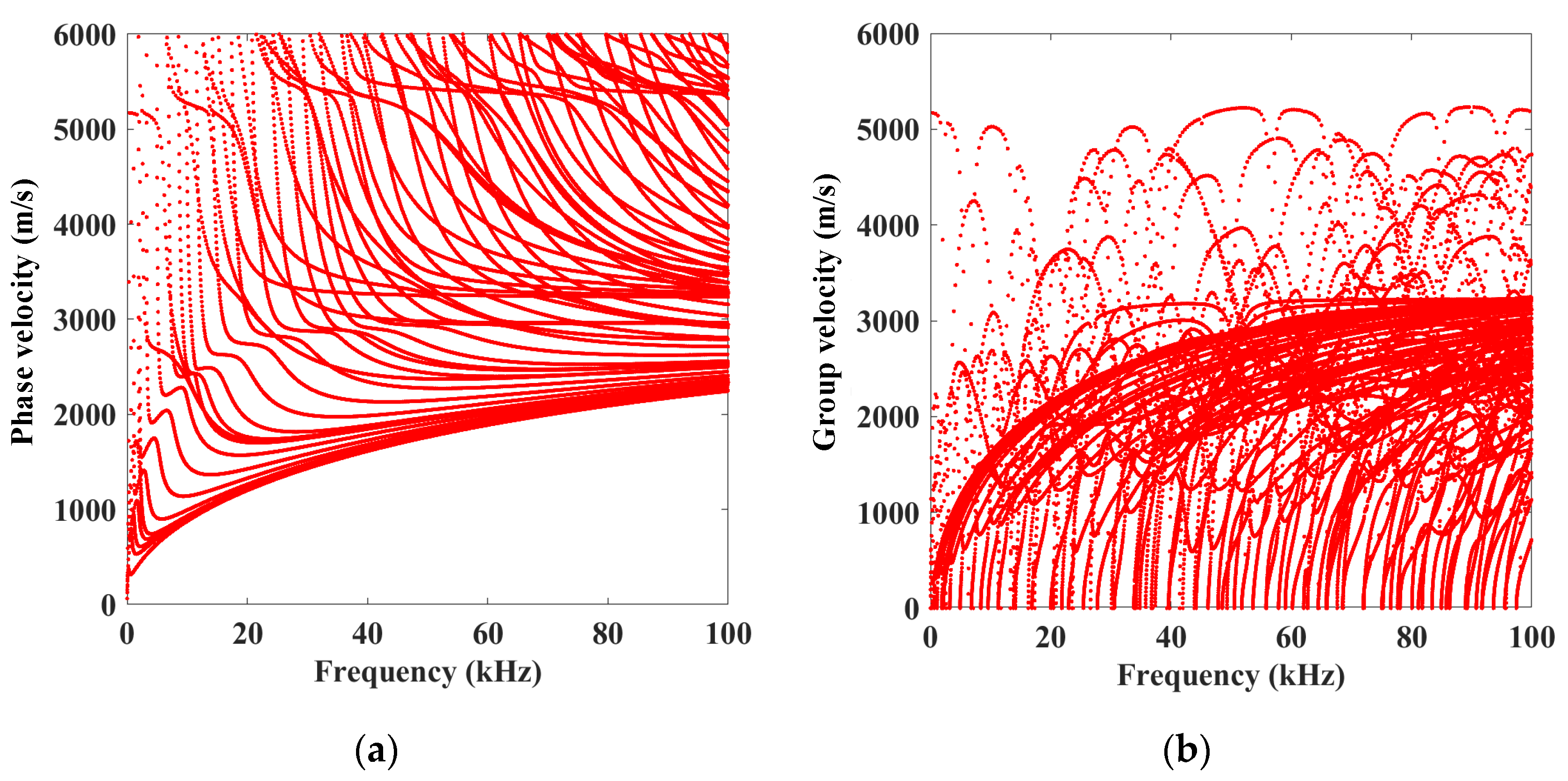
2. Dispersion Analysis of the I-Shaped Steel Beam
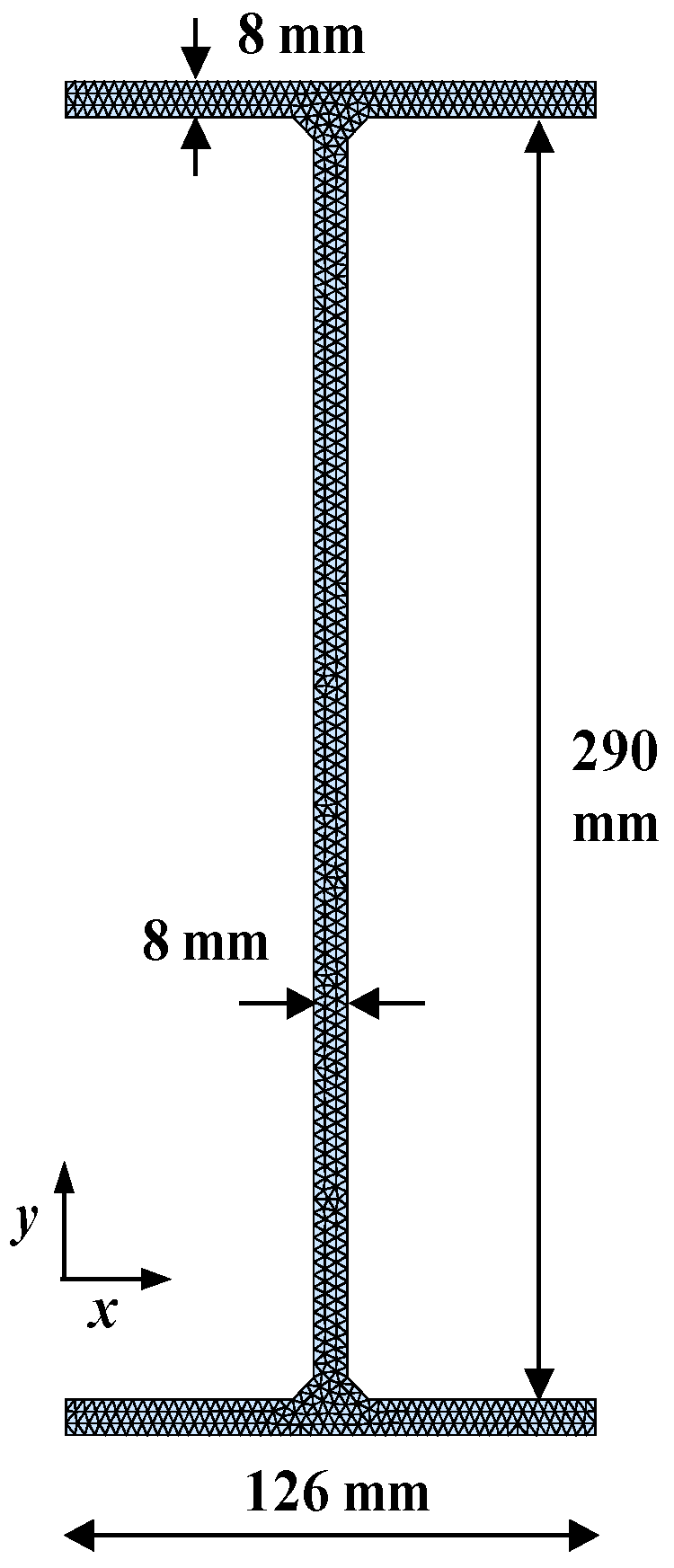
2.1. The SAFE Model

A SAFE model is constructed in the Cartesian coordinate system to calculate the dispersion curves for the I-shaped steel beam. The wave is assumed to propagate along the z axis with a harmonic exponential solution of the form e i ( k z ω t ) . k represents the wavenumber, and ω denotes the frequency. The displacement of the guided wave can be expressed as follows:
μ x ,   y ,   z ,   t = μ x x ,   y ,   z ,   t μ y x ,   y ,   z ,   t μ z x ,   y ,   z ,   t = μ x x ,   y μ y x ,   y μ z x ,   y e i ( k z ω t )
It can be observed that only the cross section requires meshing. According to the virtual work principle, the motion equation of the guided wave under the external force can be derived as
K 1 + i k K 2 + k 2 K 3 ω 2 M U = f e x
where K1, K2, and K3 are the global stiffness matrix; M is the global mass matrix; U is the global displacement matrix; and fex is the external force. To obtain the relationship between the excitation frequency (ω) and the wave number (k), Equation (2) is rewritten as follows:
A k B U ¯ = F A = 0 K 1 ω 2 M K 1 ω 2 M K ^ 2 ,   B = K 1 ω 2 M 0 0 K 3 U ¯ = U k U ,   F = 0 f e x
Given a specific frequency range, the phase velocity c p = ω / k and group velocity c g = d ω / d k can be calculated to obtain the dispersion curves. The geometrical and material parameters of the I-shaped steel beam are detailed in Table 1. Figure 1 illustrates the meshes of the cross section, which consists of 1256 triangular elements with a maximum mesh size of 2.5 mm. The phase velocity and group velocity dispersion curves of the I-shaped steel beam are shown in Figure 2, which exhibits severer dispersion than those of a plate.

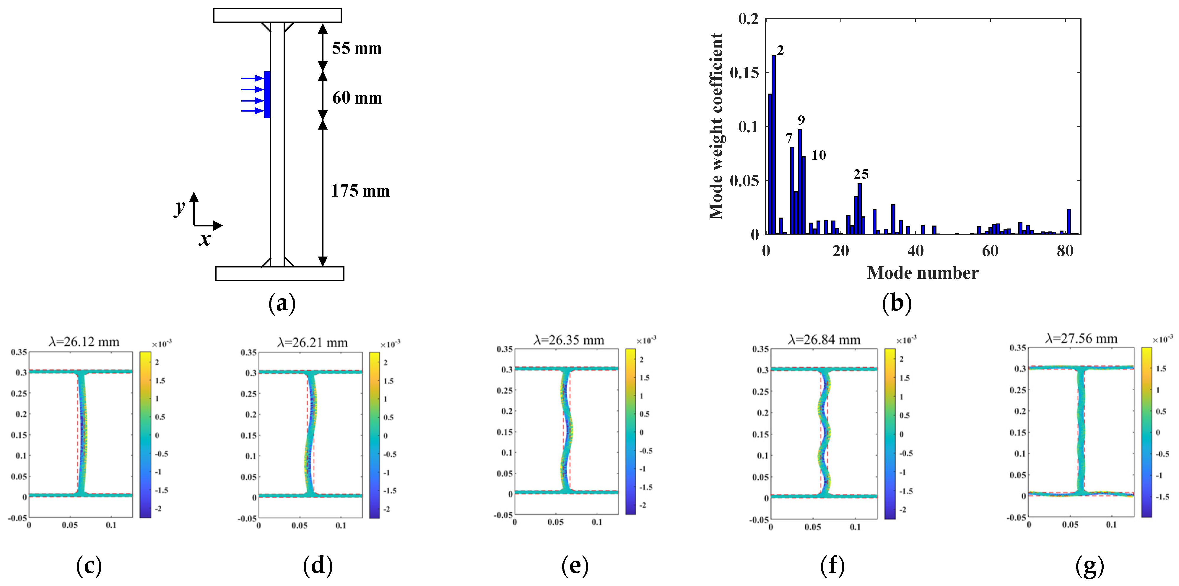
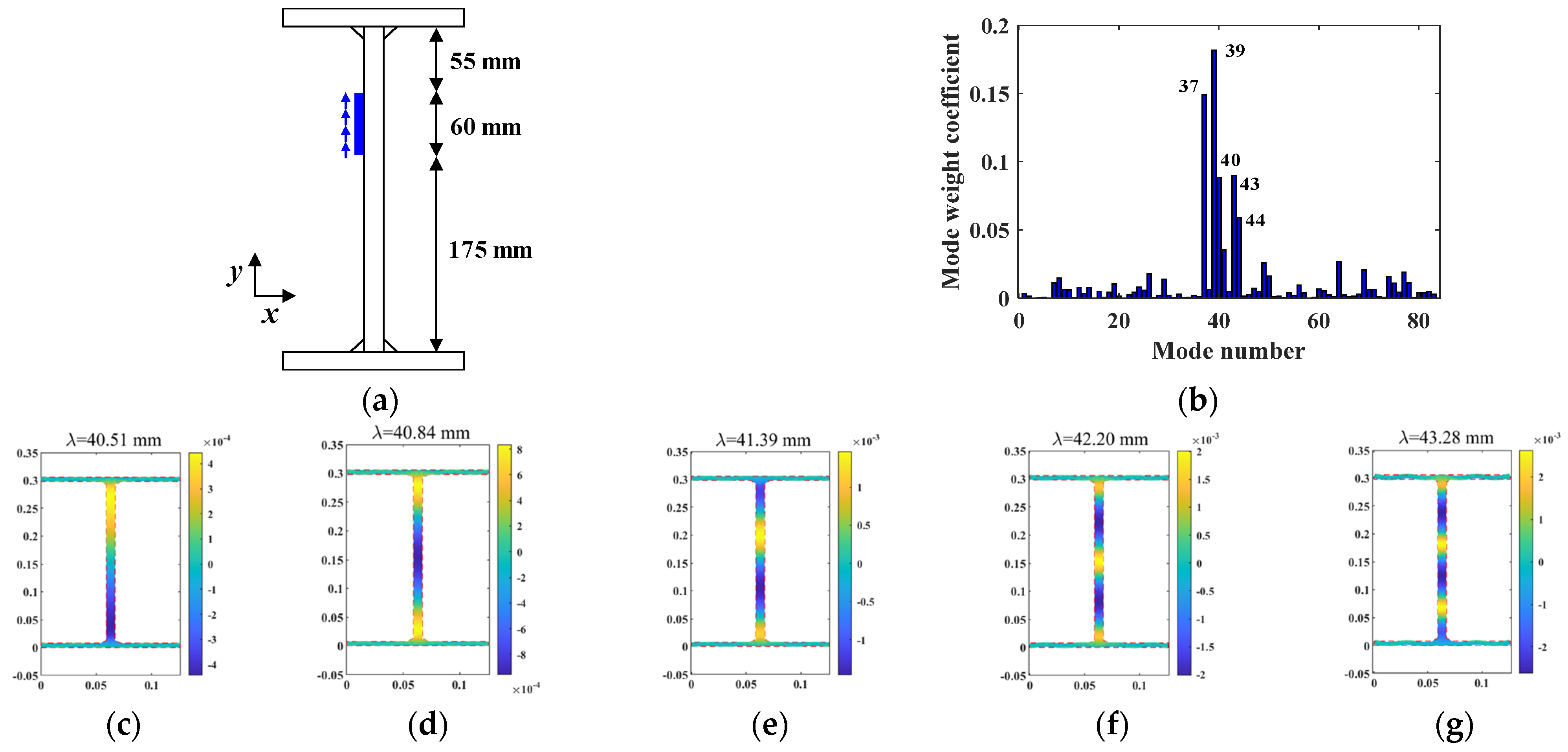
2.2. Wave Mode Analysis Under the External Load

From the dispersion curve, it can be observed that multiple modes appear at a single excitation frequency, even in the lower frequency range. The main wave modes are related to the applied external load. Supposing there are P modes at a specific excitation frequency, the mode weight coefficient (αp) for the pth mode is defined as
α p = k p Φ p f e x B p ,   B p = Φ p k p Φ p B Φ p k p Φ p T
where kp and Φ p are the wave number and mode shape of the pth mode. The location of the external force is z = zs, then the displacement U s at the position of zf in the s direction is
U s = p = 1 P α p Φ p s e i k p ( z f z s ) ( s ϵ ( x ,   y ,   z ) )
Two different loads were applied to the web in the x and y directions to simulate Lamb and SH-typed guided waves, respectively, as shown in Figure 3a and Figure 4a. The excitation frequency was determined as 80 kHz, considering the equipment and transducer conditions, and a total of 83 wave modes were identified. The distribution of αp under the two types of external loads is shown in Figure 3b and Figure 4b, with the mode shapes of the top five main modes depicted in Figure 3c–g and Figure 4c–g. Most of the wave energy is concentrated in the web for two types of external loads, although a portion of the wave energy still transfers to the flange when using the Lamb wave. The phase and group velocities of Mode 2 (the main mode under the Lamb wave) are 2097 m/s and 3142 m/s, respectively, indicating stronger dispersion, which may lead to more serious wave energy attenuation during propagation. In contrast, the phase and group velocities of Mode 39 (main mode under the SH-typed guided wave) are quite close, with values of 3267 m/s and 3191 m/s, respectively. Moreover, the present author has demonstrated that SH-typed guided waves are less affected by different surface media along the propagation path [10]. Hence, the SH-typed guided wave was adopted to detect the loosed bolts in this study.

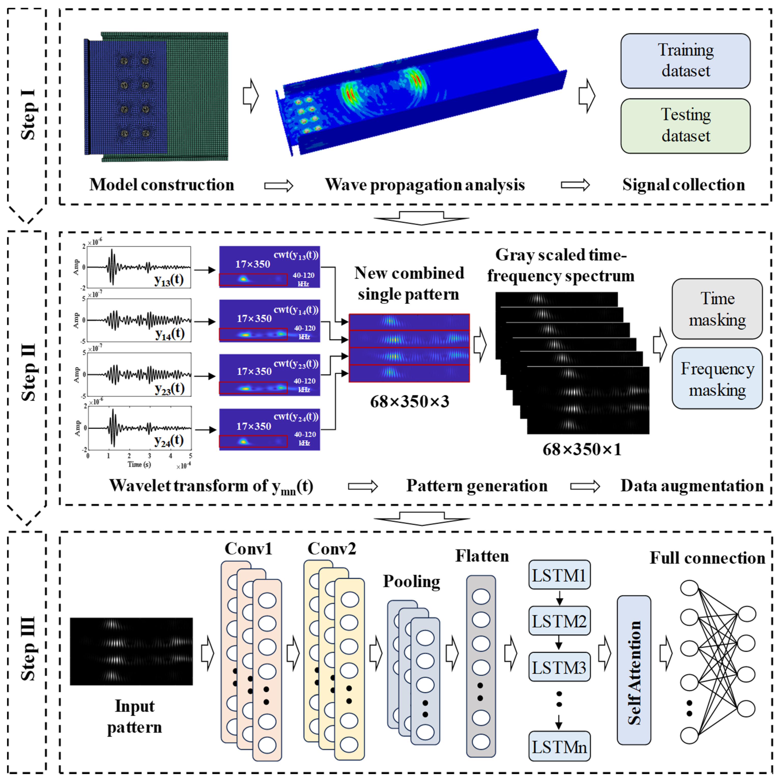
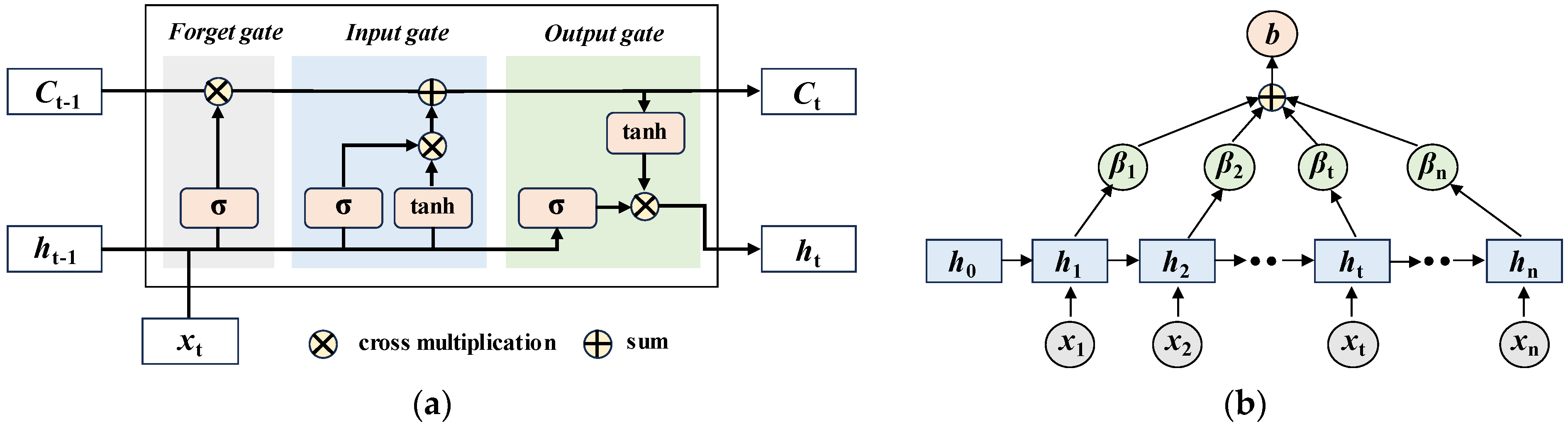
3. CNN-LSTM-MHSA Model-Based Multiple Bolt Looseness Detection

The beam–column joint used in this study is shown in Figure 5. It is composed of an I-shaped steel beam and a T-shaped steel beam. The T-shaped steel beam is attached to the column. Since this study works on detecting bolt looseness in the web of the I-shaped steel beam, the column is not simulated. Eight bolts are arranged in four rows. In this case, the limited space between the bolts and the edge of the T-shaped steel beam makes it impossible to install transducers on both sides of the bolt-connected region to receive the transmitted waves. Therefore, transducers are installed at the same side to generate and receive SH-typed guided waves. S1 and S2 work as the actuators, and S3 and S4 act as receivers. Four wave propagation paths are formed by the four transducers (S1–S3, S1–S4, S2–S3, and S2–S4). The received signal at the transducer Sn from the actuator Sm is represented as ymn(t). The generated guided wave first reaches the receiver, then passes through the bolt joint and is reflected by the end of the I-shaped steel beam. A directly incoming wave and an end-reflected wave will be captured by the receiver. The amplitude of the end-reflected wave is influenced by the contact area between the two beams, which in turn is associated with the applied bolt torque. Thus, the state of bolt connection can be judged according to the characteristic change in the received signals.
The CNN-LSTM-MHSA model is employed to locate the loosed bolt and evaluate the degree of looseness by the following steps, as illustrated in Figure 6.
Step I: A FE model of the beam–column joint is established. Numerous bolt looseness scenarios are designed to simulate different damage cases. The bolt looseness severity is adjusted by modifying the bolt tension. Subsequently, SH-typed guided wave signals are applied to the actuators to simulate the wave propagation process. For each damage case, four received signals are obtained, and the training and testing datasets are constructed under various damage cases.
Step II: Wavelet transform is applied to ymn(t) to analyze the information in the time–frequency domain. Effective regions are extracted from the time–frequency spectra of y13(t), y14(t), y23(t), and y24(t) to combine a new training pattern. The effective region should cover the directly incoming and end-reflected wave packets in the time domain and the frequency components around the central frequency of the excitation signal in the frequency domain. The new training pattern is converted to grayscale as the input to the neural network. Data augmentation techniques, including time masking and frequency masking, are then applied to the training pattern to expand the training dataset and enhance the robustness of the detection accuracy.
Step III: The CNN-LSTM-MHSA model is constructed with the combined time–frequency spectrum as the input. The CNN model consists of two conventional layers and a pooling layer, and the extracted two-dimensional features are flattened before being input to the LSTM layer. The MHSA is used to consider the inner relations between the extracted features, and fully connected layers are then conducted to map the features to the label space. In real applications, it may be challenging to detect the looseness condition of each bolt individually, so the eight bolts in the beam–column joint are segmented into four distinct subgroups by four rows. The outputs of the model are the local bolt looseness severities for the ith row (ri). ri varies from 0 (intact) to 1 (total loosed). Parameters within the neural network are updated during the training process based on the loss calculated by Equation (6) and the back propagation operation.
L o s s = 1 N j = 1 N ( 1 4 i = 1 4 ( f i j r i j ) 2 )
where N is the number of training samples, rij is the estimated local bolt looseness severity of the ith row for the jth bolt looseness case, and fij is the corresponding real value.
The traditional CNN works well for extracting spatial features from input data, while LSTM is adept at capturing long-term dependencies in time series. By combining CNN and LSTM, the model can fully process both the time and frequency information of the received guided wave signals. LSTM comprises three key components: the forget gate, the input gate, and the output gate, as shown in Figure 7a. These gates are responsible for selecting significant information from the previous time step, filtering new input information, and controlling the effective output information, respectively [39]. Since LSTM may lose important information when dealing with excessively long input sequences, CNN is utilized to reduce the dimensionality of the feature map beforehand. Figure 7b illustrates the structure of the SA mechanism, which employs probability distribution to assign higher weights to critical information, thereby enhancing model accuracy [40].

4. Numerical Example

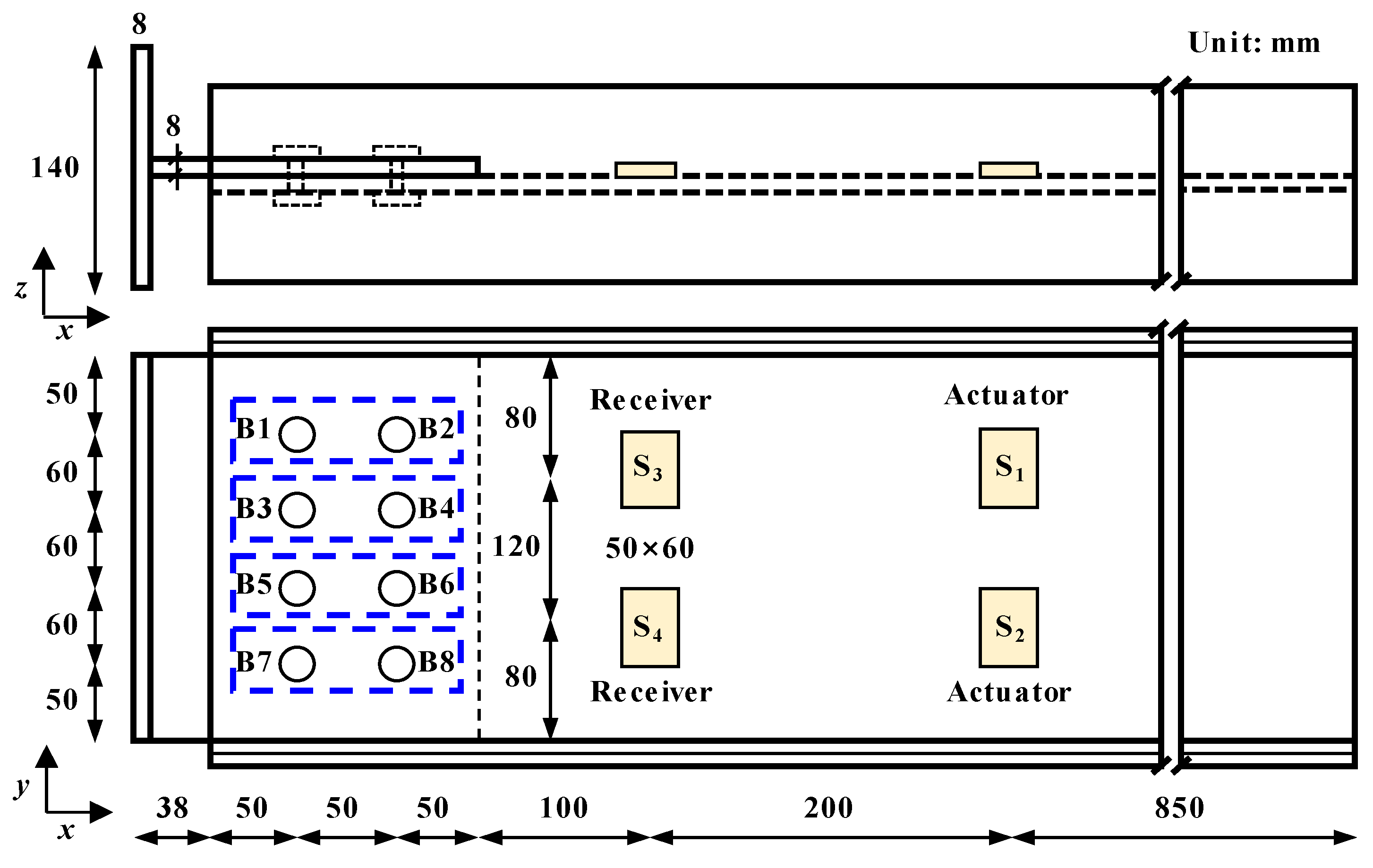
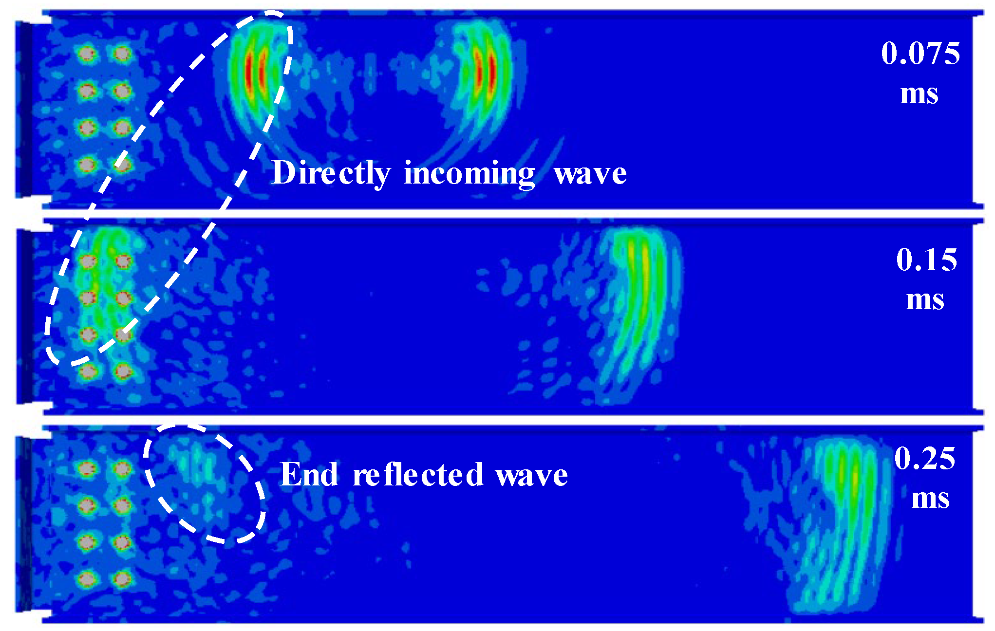
4.1. Modeling of the Beam–Column Joint

The FE model of the beam–column joint was constructed using the commercial software ABAQUS 6.14. The geometrical and material properties of the I-shaped and T-shaped steel beam are consistent with those detailed in Table 1 and Figure 5. The bolts were simulated using two bolt nuts and a bolt thread with diameter of 17 mm and 10 mm, respectively. The maximum mesh size for the beam and the bolts was set at 5 mm and 1.5 mm, with mesh refinement near the bolt of the web. The model comprises 92,160 nodes and 60,926 linear solid eight-node hexahedral elements. The contact condition between bolts and plates, as well as the contact between two plates, were modeled with hard and frictional contact in the normal and tangential directions, respectively. The friction coefficient was set to 0.3 to consider the roughness of the plates [15]. A static analysis process was initially performed to gradually add the bolt torque. The bolt torque (T) was transferred to bolt tension (F) by Equation (7). In this case, the bolt tension under the intact case was 23,000 kN, equivalent to 70% of the permissible limit.
T = K × F × d
where K is the torque quotient; d denotes the diameter of the bolt thread. Various bolt looseness conditions were simulated by changing the bolt tension. Then, an explicit dynamic analysis was conducted to model the propagation of SH-typed guided waves. The excitation signal is a three-cycle sinusoidal tone burst, with a central frequency of 80 kHz, as shown in Figure 8. SH-typed guided waves can be generated using piezoelectric transducers or magnetic effect-based transducers [41,42,43]. However, the multi-physics coupling simulations will decrease the computation efficiency. Thus, the SH-typed guided wave was generated by inducing nodal displacements at the y axis in Figure 5. A sampling frequency of 1 MHz was employed.
The distance between the actuator and the receiver in the x direction is denoted as l. The position of the receiver remains unchanged, and three different conditions with l values of 150 mm, 200 mm, and 250 mm were simulated. Figure 9 shows the received signals at the wave paths S1–S3 and S1–S4. The wave velocities for these three conditions were calculated as 3125 m/s, 3174 m/s, and 3205 m/s, respectively, which are very close to the group velocity of the main propagation mode (3191 m/s) obtained by SAFE analysis. The amplitudes of the received signals from S1–S4 were much smaller than those from S1–S3. When l equals 150 mm, the directly incoming and end-reflected wave packets are not clearly distinguishable, and the amplitude of the end-reflected wave packet starts to decrease as l is increased from 200 mm to 250 mm. Therefore, l was taken as 200 mm. The energy distribution of the SH-typed guided wave during the wave propagation process is shown in Figure 10. The SH wave reaches the left end of the I-shaped steel beam near 0.15 ms and then propagates backwards. It can be observed that the SH wave does not transmit to the flange, aligning with the wave propagation analysis results by the SAFE method.
Figure 11 illustrates the amplitude changes for four different bolt looseness scenarios, while the corresponding local bolt looseness severities are detailed in Table 2. It is assumed that the looseness severities of the two bolts are identical for each row. Cases involving different bolt looseness severities within a single row will be explored in further studies. For example, the bolt tensions for Bolt 3 to Bolt 6 were 16,100 kN in Case 1. The amplitude of the directly incoming wave remained constant across all bolt looseness cases, as it was unaffected by bolt looseness. The amplitude of the end-reflected wave packet from S1–S3 decreased as the bolt looseness severity increased, whereas the trend was reversed for the wave path S1–S4. The relative amplitude change was not quite distinct compared to those of the transmitted waves in the author’s present work [44]. So the bolt looseness severity estimation methods based on amplitude change may not be suitable in this case. The amplitudes of other wave packets situated between the directly incoming and end-reflected wave packets also exhibited changes, which could potentially carry information about bolt looseness as well. In addition, slight wave shifts were noticeable in the received signals.

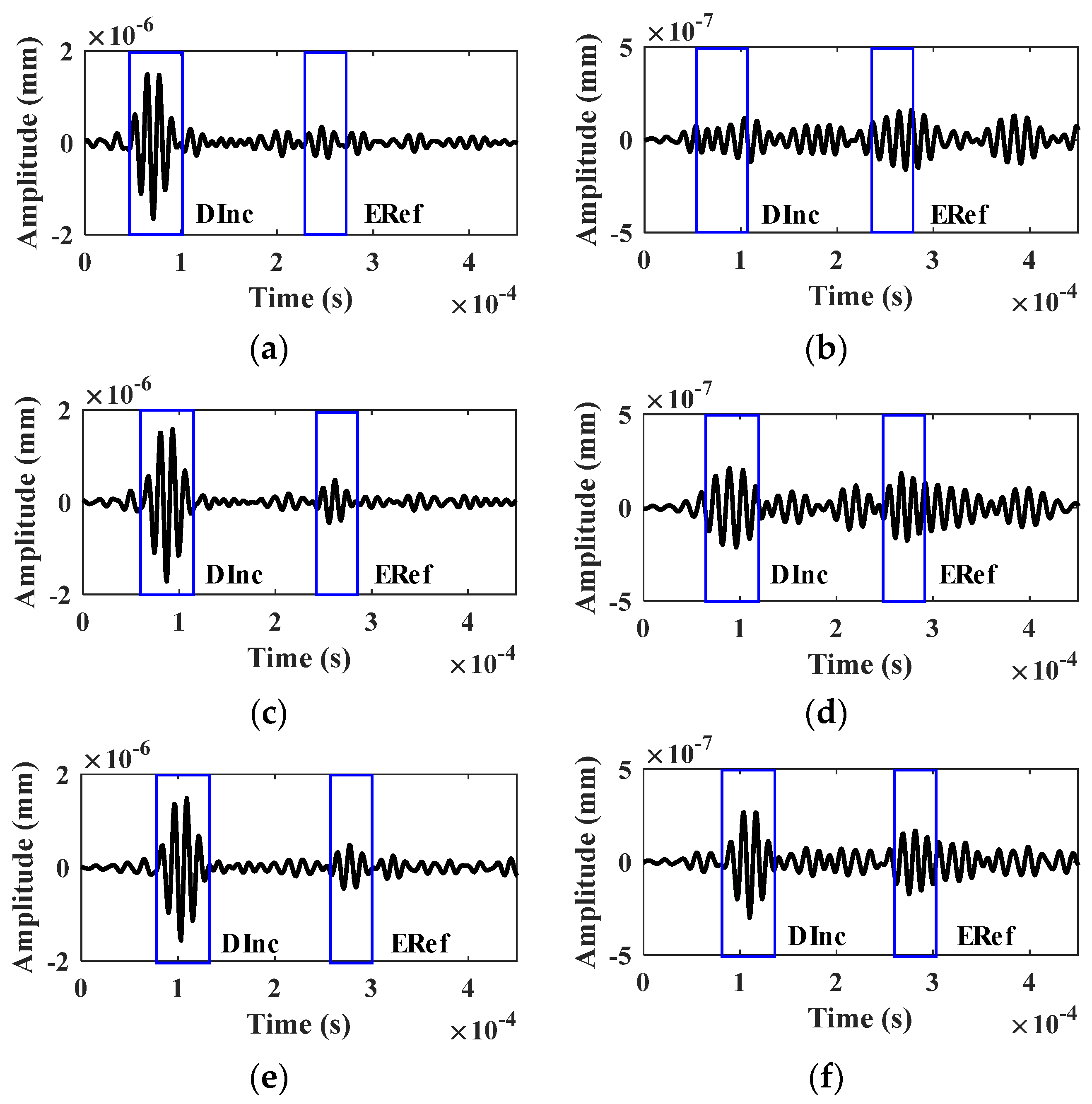
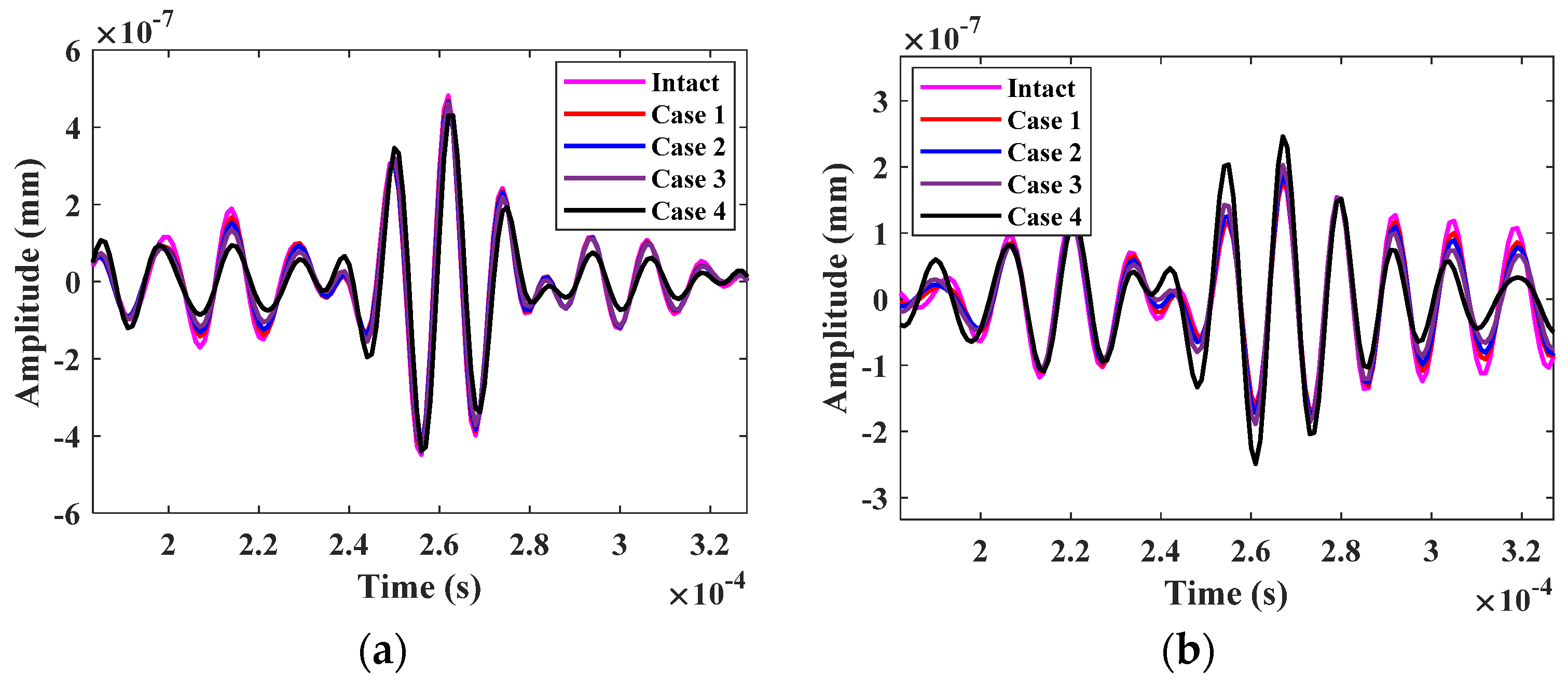
4.2. Simulation of Training and Testing Samples

The FE model was used to generate the training and testing samples. In this study, early bolt looseness conditions were considered, with the assumption that at most two out of four rows of bolts could be loosened. The local bolt looseness severity for the training samples ranged from 0 to 0.8 with an interval of 0.1, resulting in 486 ( C 4 2 × 9 × 9 ) samples. Four levels of local bolt looseness severities with fi of 0.35, 0.45, 0.55, and 0.65 were utilized for the testing samples, yielding 96 ( C 4 2 × 4 × 4 ) testing samples. An automatic sample generation program was developed by integrating ABAQUS 6.14, Python 3.9.6, and MATLAB 2023b, eliminating the need for manual GUI operations. This approach enables the collection of a large number of samples and greatly improves the computational efficiency. Details can be found in reference [44]. The received signal from each wave path underwent wavelet transform, from which the effective time–frequency region was extracted. The effective frequency range was adopted from 40 kHz to 120 kHz, considering the excitation frequency (80 kHz). The combined effective time–frequency regions from the four wave paths formed the training pattern. Figure 12 shows the combined training patterns for several bolt looseness cases, which were then converted to grayscale with dimensions of 68 × 350 × 1.

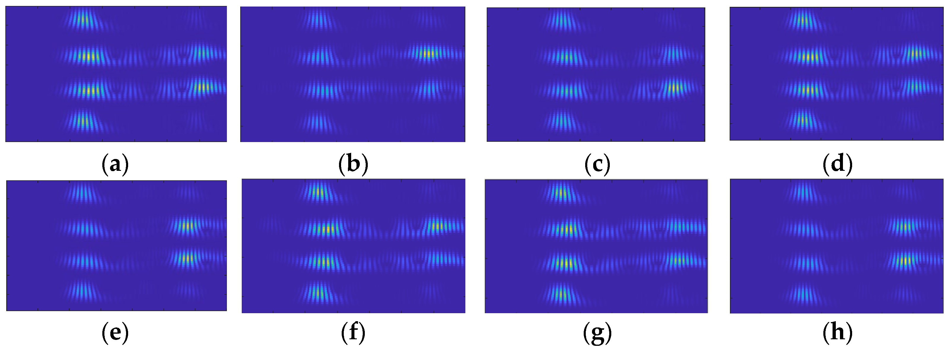
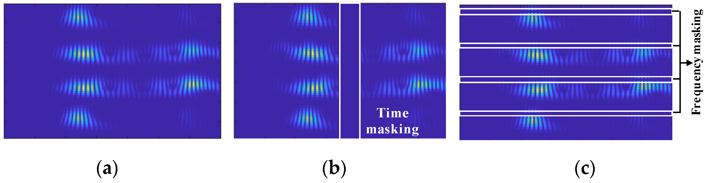
4.3. Data Augmentation

The robustness and accuracy of the deep neural network would be better if more training patterns were available for each bolt looseness case [45]. In the FE simulation, only one group of received signals was obtained for each bolt looseness case. Thus, data augmentation techniques, including time masking and frequency masking, were applied to increase the number of training patterns. Time masking was carried out on the training patterns by assigning the signal information from the four wave paths to 0 within a randomly selected time interval [ts, tf]. The maximum duration between ts and tf was 35 us, and it was ensured that [ts, tf] did not overlap with the directly incoming and end-reflected wave packets. Figure 13b shows the training pattern following the application of time masking, with the signal components within the square being masked. For frequency masking, one frequency component between 40 kHz and 120 kHz in the time–frequency spectrum from each wave propagation path was removed, excluding the range of 70 kHz to 90 kHz, which carries important information related to bolt looseness. The training pattern after frequency masking is shown in Figure 13c. The two types of data augmentation were each conducted 5 times on every training pattern, thereby increasing the total number of training patterns to 5346 (486 × 11).

5. Bolt Looseness Detection Results and Discussion

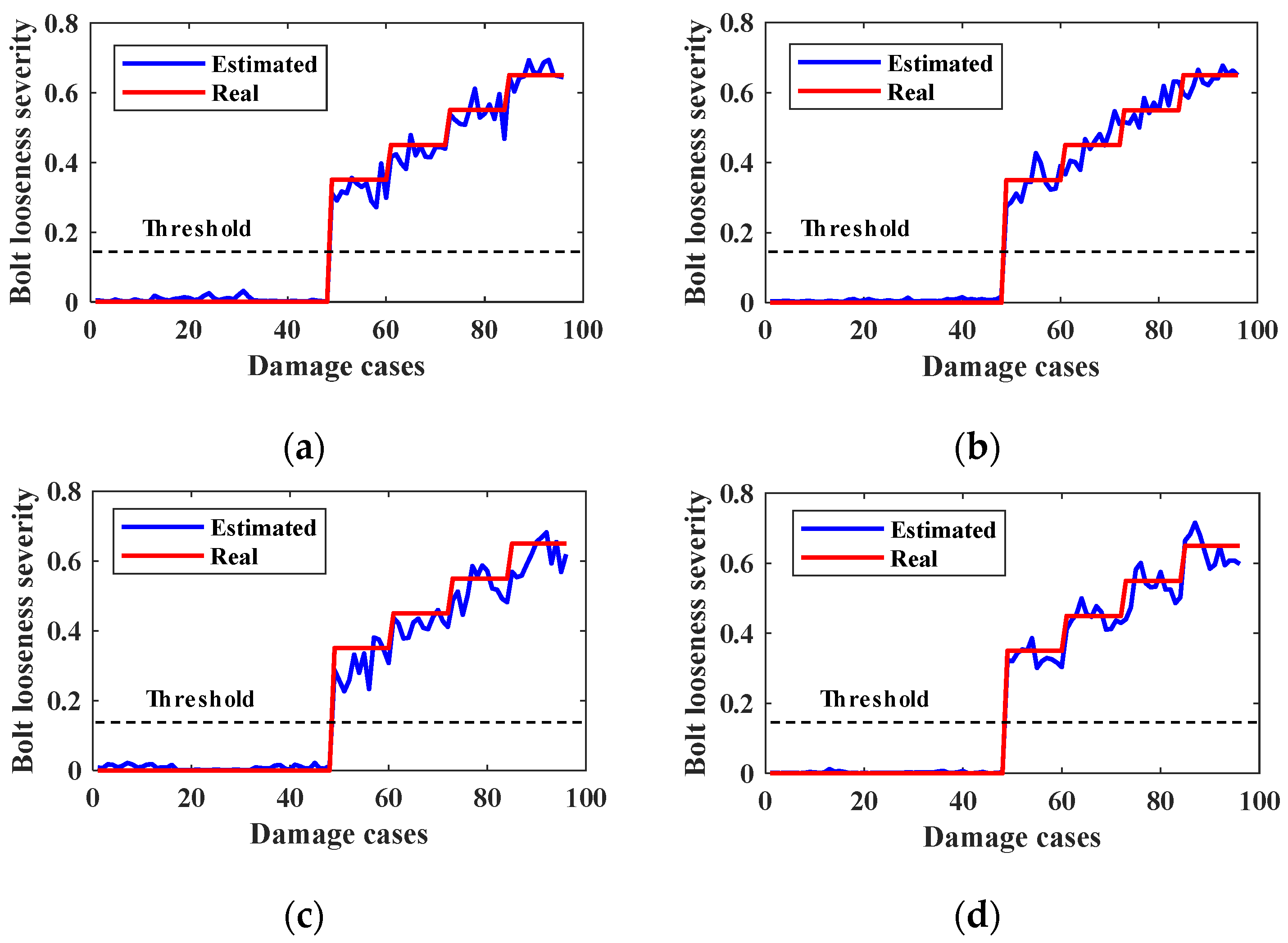
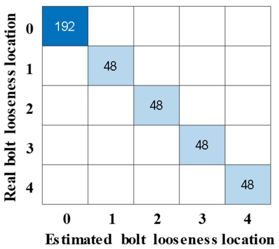
5.1. Training and Testing Results

The CNN-LSTM-MHSA network was built for estimating bolt looseness conditions based on the framework in Figure 6. The structure and detailed parameters of each layer for the neural network are listed in Table 3. A mini-batch size of 128 was used in conjunction with the Adam optimization algorithm. The training loss gradually stabilized after 30 epochs. The local bolt looseness severity estimation results for each row in the testing cases were shown in Figure 14. The estimated values coincide well with the labels, and no false, alarming, or missed detections exist. The local and overall relative error indices were defined for quantitatively accessing the bolt looseness detection accuracy as
E r r o r i l o c a l = j = 1 96 ( r i j f i j ) 2 / j = 1 96 ( 1 f i j ) 2
E r r o r o v e r a l l = j = 1 96 ( R j F j ) 2 / j = 1 96 ( 1 F j ) 2
where R j = 1 4 i = 1 4 r i j and F j = 1 4 i = 1 4 f i j are the predicted and real looseness severities of all the bolt, respectively. The calculated E r r o r i l o c a l was 3.33%, 4.0%, 5.05%, and 3.48% for four rows, with an average value of 3.96%. The E r r o r o v e r a l l was 2.09%, with the overall bolt looseness estimation result shown in Figure 15.
Figure 16 shows the bolt looseness detection results for four individual cases, indicating the excellent performance of the proposed CNN-LSTM-MHSA method. The bolt is assumed to be loosed when the estimated value exceeds 0.15. Based on this threshold, the bolt looseness localization results are categorized into four classes: TP (true positive), TN (true negative), FP (false positive), and FN (false negative). The accuracy of bolt looseness positioning was represented by the Acc value, calculated using Equation (10). Figure 17 gives the confusion matrix, and the Acc value was 100%.
A c c = T P + T N T P + F P + F N + T N

5.2. Comparison for Different Input Patterns and Other Neural Network Models

To provide a comprehensive comparison, alternative input patterns, namely time series and Fourier amplitude spectra, along with different neural network architectures, specifically CNN and CNN-LSTM, were evaluated for their effectiveness in detecting bolt looseness. For the time series input, the received signals from each wave propagation path (ymn(t)) were filtered using a bandpass filter within the range of 60 kHz to 100 kHz. Signal segments in the time duration [0, 350 us] were obtained and concatenated to create the input pattern, which has a dimension of 4 × 350. Meanwhile, the Fourier transform was applied to ymn(t), yielding Fourier amplitude spectra spanning from 0 to 194 kHz. These spectra were utilized to construct the frequency-domain training pattern, sized 4 × 200. These input patterns, derived from time series, Fourier amplitude spectra, and time–frequency spectra, were fed into CNN, CNN-LSTM, and CNN-LSTM-MHSA models to assess their accuracy in estimating bolt looseness conditions. Given the dimensions of the above two types of training patterns, the kernel sizes for two convolutional layers, and the max-pooling layer were set to 1 × 4 and 1 × 1, respectively, with other hyperparameters fine-tuned for optimal performance. The outcomes of bolt looseness localization and severity estimation are listed in Table 4. Among the models tested, the CNN-LSTM-MHSA model, when supplied with time–frequency spectrum inputs, demonstrated superior performance.
The proposed method was also compared with the wave energy-based method as in the author’s previous work [44]. The wave energy reflection coefficient ( I R E F , i j ) on the wave path Si–Sj is defined based on the wave energies from the directly incoming ( E i j i n c ) and end-reflected ( E i j r e f ) wave packets as follows:
I R E F , i j = E i j r e f / E i j i n c
The method of calculating wave energies can refer to [44]. I R E F , i j was normalized using the wave energy reflection coefficient in the undamaged case ( I R E F , i j 0 ) as
I R E F , i j n o r = I R E F , i j 0 / I R E F , i j
A BPNN was designed, taking as input the four I R E F , i j n o r values from the four wave paths, with the outputs representing the damage severities of each row (ri). There were two hidden layers with six neural nodes in each layer. Errorlocal and Erroroverall were calculated as 6.3% and 2.5%, respectively, and the Acc value was 99.20%.

5.3. Noise Injection Testing

Measurement noise significantly impacts bolt looseness detection accuracy, particularly when dealing with time series data or normalized wave energy reflection ratios. Noise injection testing was carried out to test the robustness of the proposed method by adding white noise to the received signals. For the training and testing signals, white noise levels of 10% and 20% of the signal’s RMS value were considered, corresponding to signal-to-noise ratios of 10 dB and 7 dB, respectively. Figure 18 shows the received signal at S1–S3 with 10% and 20% noise under the intact case. The bolt looseness condition estimation results for the CNN-LSTM-MHSA method under various noise levels are summarized in Table 5. For the cases with 10% and 20% of white noise in the training dataset, the bolt looseness localization accuracy decreased slightly for testing samples without noise. The bolt looseness localization accuracy remained excellent by increasing noise level in the testing samples, and the local bolt looseness severity estimation accuracy decreased in an acceptable range. In real applications, obtaining numerous training samples with varying bolt looseness scenarios can be challenging. Utilizing the CNN-LSTM-MHSA method trained with FE simulation results to test measurement data may address this issue. Incorporating different levels of noise into the training dataset to account for the noise effect and improve detection accuracy will be explored in future studies.

6. Conclusions

This study presented a CNN-LSTM-MHSA-based method for the quantitative assessment of bolt looseness in a beam–column joint connected by multiple bolts. A SAFE model was constructed to analyze the wave propagation properties of Lamb waves and SH-typed guided waves in an I-shaped steel beam. Two pairs of transducers were utilized for generating and receiving the SH waves across four distinct wave paths, and the time–frequency information was collected and combined to obtain the input pattern required for the deep neural network. Numerical simulations were conducted to verify the SAFE analysis results and collect samples with varying bolt looseness conditions. Data augmentation techniques were employed to expand the training dataset. Comparative studies and noise injection testing were carried out to evaluate the performance of the proposed method. The following conclusions have been drawn:
(1)
The proposed mode weight coefficient aids in understanding how wave modes are distributed under different external loads for the I-shaped steel beam with complex dispersion properties. This coefficient can also assist in selecting the appropriate mode and position for the excitation signal.
(2)
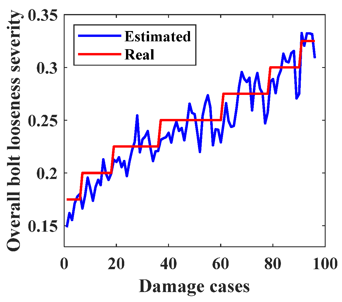
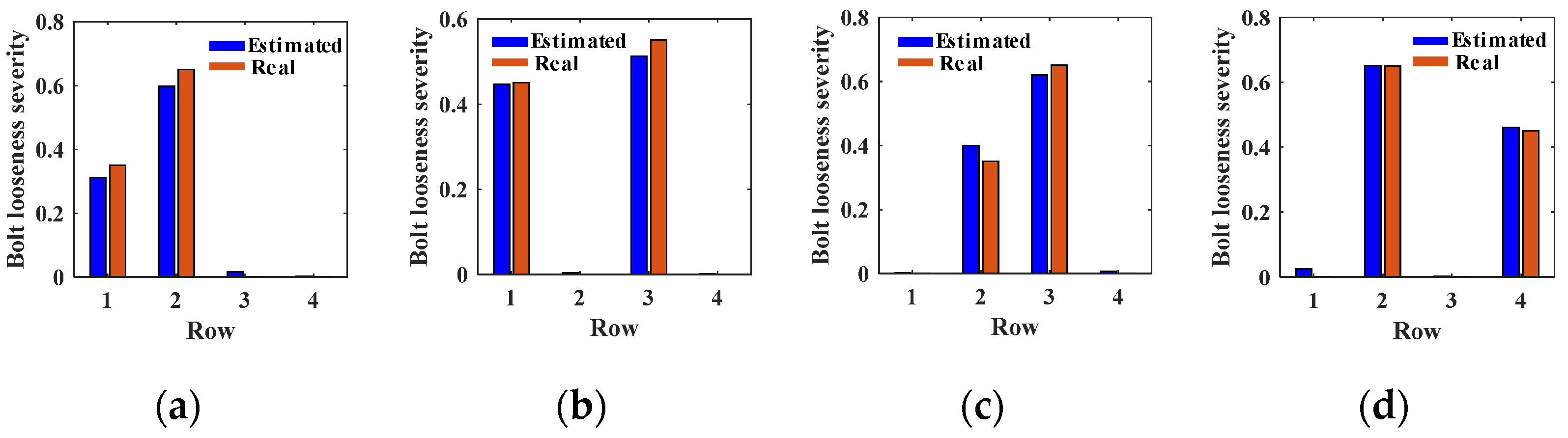
The looseness conditions of multiple bolts in the beam–column joint were easily detected using the proposed CNN-LSTM-MHSA model. The bolt looseness localization accuracy was 100%, with local and overall severity estimation errors of 3.96% and 2.09%, respectively.
(3)
The CNN-LSTM-MHSA model, which integrates the time–frequency spectrum extracted from the guided wave signals, outperformed traditional deep neural networks with inputs of time series data and Fourier amplitude spectra, as well as the wave energy reflection ratio-based method.
(4)
White noise levels of 10% and 20% were added to the training and testing samples to simulate the effects of measurement noise. The proposed method maintained good bolt looseness localization accuracy, with values exceeding 93%. The maximum errors for Errorlocal and Erroroverall were 17.24% and 7.57%, respectively.
Experimental studies and real applications will be carried out for the beam–column joint later. For laboratory tests, the bolt looseness scenarios considered in the FE simulations will be conducted on a beam–column joint with the same dimensions. The received signals will be measured by the magnetostrictive transducer and used to train the CNN-LSTM-MHSA model in order to verify the proposed method. However, it is not easy to acquire enough training samples with desirable bolt looseness conditions in real applications. Testing the experimental data using the neural network trained by the FE simulations may solve this problem. Thus, the FE model should be well modified according to the experimental data. Additionally, the influence of uncertain factors, such as temperature changes and the surface roughness of plates, on the detection accuracy will be investigated experimentally.

Author Contributions

Conceptualization, R.Z., X.S., Y.D. and Y.L.; methodology, X.S.; investigation, Y.F. and R.M.; data curation, X.S.; writing—original draft preparation, X.S.; writing—review and editing, R.Z., Y.D. and Y.L.; visualization, Y.F.; supervision, Y.D. and Y.L.; funding acquisition, R.Z., X.S. and Y.D. All authors have read and agreed to the published version of the manuscript.

Funding

This research was funded by the National Natural Science Foundation of China (Grant Nos. U24A20169, 51608478), the Zhejiang Provincial Natural Science Foundation of China (Grant No. LGG21E080004), and the Scientific Research Fund of Zhejiang Provincial Education Department (Grant No. Y202454348).

Institutional Review Board Statement

Not applicable.

Informed Consent Statement

Not applicable.

Data Availability Statement

The original contributions presented in this study are included in the article. Further inquiries can be directed to the corresponding author.

Conflicts of Interest

The authors declare no conflicts of interest.

References

  1. Nguyen, T.T.; Ta, Q.B.; Ho, D.D.; Kim, J.T.; Huynh, T.C. A method for automated bolt-loosening monitoring and assessment using impedance technique and deep learning. Dev. Built Environ. 2023, 14, 100122. [Google Scholar] [CrossRef]
  2. Chelimilla, N.; Chinthapenta, V.; Kali, N.; Korla, S. Review on recent advances in structural health monitoring paradigm for looseness detection in bolted assemblies. Struct. Health Monit. 2023, 22, 4264–4304. [Google Scholar] [CrossRef]
  3. Bonab, B.T.; Sadeghi, M.H.; Ettefagh, M.M. Bolt looseness detection in flanged pipes using parametric modeling. J. Pipeline Syst. Eng. Pract. 2024, 16, 04024067. [Google Scholar] [CrossRef]
  4. Huynh, T.C. Vision-based autonomous bolt-looseness detection method for splice connections: Design, lab-scale evaluation, and field application. Automat. Constr. 2021, 124, 103591. [Google Scholar] [CrossRef]
  5. Zhou, L.; Chen, S.X.; Ni, Y.Q.; Choy, A.W.H. EMI-GCN: A hybrid model for real-time monitoring of multiple bolt looseness using electromechanical impedance and graph convolutional networks. Smart Mater. Struct. 2021, 30, 035032. [Google Scholar] [CrossRef]
  6. Chen, D.D.; Li, W.; Dong, Z.Q.; Fu, R.L.; Yu, Q. Multi-bolt looseness monitoring using guided waves: A cross-correlation approach of the wavelet energy envelope. Smart Mater. Struct. 2024, 33, 125019. [Google Scholar] [CrossRef]
  7. Wang, X.; Yue, Q.R.; Liu, X.G. Bolted lap joint loosening monitoring and damage identification based on acoustic emission and machine learning. Mech. Syst. Signal Process. 2024, 220, 111690. [Google Scholar] [CrossRef]
  8. Mori, K.; Horibe, T.; Maejima, K. Evaluation of the axial force in an FeCo bolt using the inverse magnetostrictive effect. Measurement 2020, 165, 108131. [Google Scholar] [CrossRef]
  9. Allen, J.C.P.; Ng, C.T. Nonlinear guided-wave mixing for condition monitoring of bolted joints. Sensors 2021, 21, 5093. [Google Scholar] [CrossRef]
  10. Zhang, M.R.; Tang, Z.F.; Yun, C.B.; Sui, X.D.; Chen, J.; Duan, Y.F. Bolt looseness detection using SH guided wave and wave energy transmission. Smart Mater. Struct. 2021, 30, 105015. [Google Scholar] [CrossRef]
  11. Zhang, Y.; Liu, J.H.; Cui, X.S.; Li, D.S. Guided wave-based damage assessment on bolt in precast beam-to-column joints. J. Build. Eng. 2024, 87, 108998. [Google Scholar] [CrossRef]
  12. Kitazawa, S.; Lee, Y.; Patel, R. Noncontact measurement of bolt axial force in tightening processes using scattered laser ultrasonic waves. NDT E Int. 2023, 137, 102838. [Google Scholar] [CrossRef]
  13. Du, F.; Wu, S.W.; Sheng, R.Z.; Xu, C.; Gong, H.; Zhang, J. Investigation into the transmission of guided waves across bolt jointed plates. Appl. Acoust. 2022, 196, 108866. [Google Scholar] [CrossRef]
  14. Wang, T.; Liu, S.P.; Shao, J.H.; Li, Y.R. Health monitoring of bolted joints using the time reversal method and piezoelectric transducers. Smart Mater. Struct. 2016, 25, 025010. [Google Scholar]
  15. Parvasi, S.M.; Ho, S.C.M.; Kong, Q.; Mousavi, R.; Song, G. Real time bolt preload monitoring using piezoceramic transducers and time reversal technique-a numerical study with experimental verification. Smart Mater. Struct. 2016, 25, 085015. [Google Scholar] [CrossRef]
  16. Xu, C.; Wu, G.N.; Du, F.; Zhu, W.D.; Mahdavi, S.H. A modified time reversal method for guided wave based bolt loosening monitoring in a lap joint. J. Nondestruct. Eval. 2019, 38, 85. [Google Scholar] [CrossRef]
  17. Qiu, J.X.; Abbas, S.; Zhu, Y.P.; Abbas, Z. Integrated acoustic-vibration frequency-modulation technology to detect the contact nonlinear features of mechanical structure. Struct. Control Health Monit. 2022, 29, e3057. [Google Scholar] [CrossRef]
  18. Chen, D.D.; Zhang, N.N.; Huo, L.S.; Song, G.B. Full-range bolt preload monitoring with multi-resolution using the time shifts of the direct wave and coda waves. Struct. Health Monit. 2023, 22, 3871–3890. [Google Scholar] [CrossRef]
  19. Hayashi, T.; Tamayama, C.; Murase, M. Wave structure analysis of guided waves in a bar with an arbitrary cross-section. Ultrasonics 2006, 44, 17–24. [Google Scholar] [CrossRef]
  20. Shen, W.; Li, D.S.; Ou, J.P. Dispersion analysis of multiscale wavelet finite element for 2D elastic wave propagation. J. Eng. Mech. 2020, 146, 04020022. [Google Scholar] [CrossRef]
  21. Tu, J.Q.; Tang, Z.F.; Yun, C.B.; Wu, J.J.; Xu, X. Guided wave-based damage assessment on welded steel I-beam under ambient temperature variations. Struct. Control Health Monit. 2021, 28, e2696. [Google Scholar] [CrossRef]
  22. Daneshyar, A.; Sotoudeh, P.; Ghaemian, M. The scaled boundary finite element method for dispersive wave propagation in higher-order continua. Int. J. Numer. Methods Eng. 2023, 124, 880–927. [Google Scholar] [CrossRef]
  23. Nemer, R.; Bouchoucha, F.; Arfa, H.; Ichchou, M. Wave propagation in uncertain laminated structure through stochastic wave finite element method. Mech. Res. Commun. 2025, 143, 104350. [Google Scholar] [CrossRef]
  24. Wu, J.J.; Tang, Z.F.; Lv, F.Z.; Yang, K.J. Ultrasonic guided wave focusing in waveguides with constant irregular cross-sections. Ultrasonics 2018, 89, 1–12. [Google Scholar] [CrossRef]
  25. Tang, Z.F.; Sui, X.D.; Duan, Y.F.; Zhang, P.F.; Yun, C.B. Guided wave-based cable damage detection using wave energy transmission and reflection. Struct. Control Health Monit. 2021, 28, e2688. [Google Scholar] [CrossRef]
  26. Li, W.X.; Dwight, R.A.; Zhang, T.L. On the study of vibration of a supported railway rail using the semi-analytical finite element method. J. Sound Vib. 2015, 345, 121–145. [Google Scholar] [CrossRef]
  27. Mariani, S.; Palermo, A.; Marzani, A. An extended semi-analytical finite element method for modeling guided waves in plates with pillared metasurfaces. J. Sound Vib. 2025, 607, 119030. [Google Scholar] [CrossRef]
  28. Khurjekar, I.D.; Harley, J.B. Reliability assessment of guided wave damage localization with deep learning uncertainty quantification methods. NDT E Int. 2024, 144, 103099. [Google Scholar] [CrossRef]
  29. Yuan, R.; Lv, Y.; Kong, Q.Z.; Song, G.B. Percussion-based bolt looseness monitoring using intrinsic multiscale entropy analysis and BP neural network. Smart Mater. Struct. 2019, 28, 125001. [Google Scholar] [CrossRef]
  30. Duan, Y.F.; Sui, X.D.; Tang, Z.F.; Yun, C.B. Bolt looseness detection and localization using time reversal signal and neural network techniques. Smart Struct. Syst. 2022, 30, 397–410. [Google Scholar]
  31. Wang, F.R.; Mobiny, A.; Nguyen, H.V.; Song, G.B. If structure can exclaim: A novel robotic-assisted percussion method for spatial bolt-ball joint looseness detection. Struct. Health Monit. 2021, 20, 1597–1608. [Google Scholar] [CrossRef]
  32. Chen, Y.X.; Zhu, L.; Gao, Z.N.; Li, W.J.; Wu, J.C. Multi-bolt looseness positioning using multivariate recurrence analytic active sensing method and MHAMCNN model. Struct. Health Monit. 2025, 24, 812–829. [Google Scholar] [CrossRef]
  33. Sui, X.D.; Zhang, R.; Luo, Y.Z.; Fang, Y. Multiple bolt looseness detection using SH-typed guided waves: Integrating physical mechanism with monitoring data. Ultrasonics 2025, 150, 107601. [Google Scholar] [CrossRef] [PubMed]
  34. Wang, F.R.; Song, G.B. A novel percussion-based method for multi-bolt looseness detection using one-dimensional memory augmented convolutional long short-term memory networks. Mech. Syst. Signal Process. 2021, 161, 107955. [Google Scholar] [CrossRef]
  35. Ding, Y.; Ye, X.W.; Su, Y.H. Wind-induced fatigue life prediction of bridge hangers considering the effect of wind direction. Eng. Struct. 2025, 327, 119523. [Google Scholar] [CrossRef]
  36. Zhang, X.L.; Xia, Y.; Zhao, J.F. Intelligent identification of bolt looseness with one-dimensional deep convolutional neural networks. Signal Image Video Process. 2025, 19, 158. [Google Scholar] [CrossRef]
  37. Yu, K.; Lin, T.R.; Ma, H.; Li, X.; Li, X. A multi-stage semi-supervised learning approach for intelligent fault diagnosis of rolling bearing using data augmentation and metric learning. Mech. Syst. Signal Process. 2021, 146, 107043. [Google Scholar] [CrossRef]
  38. Hu, T.H.; Tang, T.; Lin, R.L.; Chen, M.; Han, S.F.; Wu, J. A simple data augmentation algorithm and a self-adaptive convolutional architecture for few-shot fault diagnosis under different working conditions. Measurement 2020, 156, 107539. [Google Scholar] [CrossRef]
  39. Zayat, A.; Obeed, M.; Chaaban, A. Diversion detection in small-diameter HDPE pipes using guided waves and deep learning. Sensors 2022, 22, 9586. [Google Scholar] [CrossRef]
  40. Ghazimoghadam, S.; Hosseinzadeh, S.A.A. A novel unsupervised deep learning approach for vibration-based damage diagnosis using a multi-head self-attention LSTM autoencoder. Measurement 2024, 229, 114410. [Google Scholar] [CrossRef]
  41. Seung, H.M.; Kim, H.W.; Kim, Y.Y. Development of an omni-directional shear-horizontal wave magnetostrictive patch transducer for plates. Ultrasonics 2013, 53, 1304–1308. [Google Scholar] [CrossRef] [PubMed]
  42. Alam, Z.; Sharma, A.K. Topology optimization of hard-magnetic soft laminates for wide tunable SH wave bandgaps. Compos. Struct. 2025, 366, 119157. [Google Scholar] [CrossRef]
  43. Sui, X.D.; Zhang, R.; Luo, Y.Z.; Tang, Z.F.; Wang, Z. A Lorentz force-based SH-typed electromagnetic acoustic transducer using flexible circumferential printed circuit. Ultrasonics 2024, 141, 107348. [Google Scholar] [CrossRef] [PubMed]
  44. Sui, X.D.; Duan, Y.F.; Yun, C.B.; Tang, Z.F.; Chen, J.W.; Shi, D.W.; Hu, G.M. Bolt looseness detection and localization using wave energy transmission ratios and neural network technique. J. Infrastruct. Intell. Resil. 2023, 2, 100025. [Google Scholar] [CrossRef]
  45. Du, F.; Wu, S.W.; Tian, Z.X.; Qiu, F.; Xu, C.; Su, Z.Q. An improved prototype network and data augmentation algorithm for few-shot structural health monitoring using guided waves. IEEE Sens. J. 2023, 23, 8714–8726. [Google Scholar] [CrossRef]
Figure 1. Cross section and meshes of the I-shaped steel beam.
Applsci 15 06425 g001
Figure 2. Dispersion curves of the I-shaped steel beam. (a) Phase velocity; (b) group velocity.
Applsci 15 06425 g002
Figure 3. Wave mode component analysis by applying external load in the x direction (simulation of Lamb wave). (a) External load in the x direction. (b) Distribution of αp. (c) Mode 1. (d) Mode 2. (e) Mode 7. (f) Mode 9. (g) Mode 10.
Applsci 15 06425 g003
Figure 4. Wave mode component analysis by applying external load in the y direction (simulation of SH-typed guided wave). (a) External load in the y direction. (b) Distribution of αp. (c) Mode 37. (d) Mode 39. (e) Mode 40. (f) Mode 43. (g) Mode 44.
Applsci 15 06425 g004
Figure 5. Diagram of the tested beam–column joint.
Applsci 15 06425 g005
Figure 6. Implementation flow of the proposed method.
Applsci 15 06425 g006
Figure 7. Structure of the LSTM and SA mechanism. (a) LSTM cell; (b) SA mechanism.
Applsci 15 06425 g007
Figure 8. The three-cycle tone burst excitation signal. (a) times history; (b) FFT.
Applsci 15 06425 g008
Figure 9. Received signals under different transducer configurations (DInc: directly incoming wave packet; ERef: end-reflected wave packet). (a) S1–S3 (l = 150 mm); (b) S1–S4 (l = 150 mm); (c) S1–S3 (l = 200 mm); (d) S1–S4 (l = 200 mm); (e) S1–S3 (l = 250 mm); (f) S1–S4 (l = 250 mm).
Applsci 15 06425 g009
Figure 10. Energy distribution during wave propagation (l = 200 mm).
Applsci 15 06425 g010
Figure 11. Changes in the end-reflected wave packet under different bolt looseness severities (l = 200 mm). (a) S1–S3; (b) S1–S4.
Applsci 15 06425 g011
Figure 12. The reconstructed time–frequency spectrums for some training samples. (a) {0, 0.5, 0, 0}; (b) {0, 0, 0, 0.7}; (c) {0.3, 0.4, 0, 0}; (d) {0, 0.2, 0.6, 0}; (e) {0, 0.5, 0, 0.4}; (f) {0.3, 0, 0.4, 0}; (g) {0.6, 0, 0, 0.3}; (h) {0, 0, 0.2, 0.8}.
Applsci 15 06425 g012
Figure 13. Data augmentation on the training pattern. (a) Original pattern; (b) after time masking; (c) after frequency masking.
Applsci 15 06425 g013
Figure 14. Bolt looseness severity evaluation results for each row. (a) f1j for Row 1; (b) f2j for Row 2; (c) f3j for Row 3; (d) f4j for Row 4.
Applsci 15 06425 g014
Figure 15. Overall bolt looseness severity estimation results.
Applsci 15 06425 g015
Figure 16. Quantitative detection results for individual cases. (a) {0.35,0.65,0,0}; (b) {0.45,0,0.55,0}; (c) {0,0.35,0.65,0}; (d) {0,0.65,0,0.45}.
Applsci 15 06425 g016
Figure 17. Damage localization result (0 means intact).
Applsci 15 06425 g017
Figure 18. The received signal at S1–S3 with white noise under the intact case. (a) 10%; (b) 20%.
Applsci 15 06425 g018
Table 1. The material and geometrical properties of the I-shaped steel beam.
Young’s ModulusDensityPoisson RatioWidth of FlangeHeight of WebThickness of Flange and Web
210 GPa7800 kg/m30.28126 mm290 mm8 mm
Table 2. Description of damage severity for four example cases.
Damage Cases{f} = {f1, f2, f3, f4}
Case 1{0, 0.3, 0.3, 0}
Case 2{0, 0.45, 0.45, 0}
Case 3{0, 0.6, 0.6, 0}
Case 4{0, 0.75, 0.75, 0}
Table 3. Details of the CNN-LSTM-MHSA network.
LayerActive FunctionSizeRemarks
Conv1ReLU16 × [3, 4]Padding: same
Conv2ReLU32 × [3, 4]Padding: same
Max-poolingReLU[2, 2]Padding: same
Stride: 2 × 2
Flatten---
LSTM-24Number of hidden units
MHSA-8 × 24-
Fully connected1ReLU128-
Fully connected2Sigmoid4-
Table 4. Comparison for bolt looseness detection using different input patterns and neural network models.
Neural Network and Evaluation IndexTime SeriesFourier Amplitude SpectrumTime–Frequency Spectrum
CNNAcc97.39%99.48%99.74%
Errorlocal13.40%6.84%7.53%
Erroroverall7.70%5.09%3.94%
CNN-LSTMAcc99.74%100%100%
Errorlocal7.44%5.85%4.88%
Erroroverall4.44%3.27%2.50%
CNN-LSTM-MHSAAcc100%100%100%
Errorlocal5.96%5.98%3.96%
Erroroverall3.79%2.83%2.09%
Note: Errorlocal is the average value of E r r o r i l o c a l
Table 5. Noise injection testing results of the CNN-LSTM-MHSA method.
Noise in the Testing SamplesCNN-LSTM-MHSA Trained with 10% Noise
AccErrorlocalErroroverall
No99.48%8.90%5.60%
10%97.92%12.42%6.23%
20%93.48%17.24%7.57%
Noise in the Testing SamplesCNN-LSTM-MHSA Trained with 20% Noise
AccErrorlocalErroroverall
No99.74%7.43%3.97%
10%97.40%11.43%6.03%
20%97.14%16.09%7.57%
Disclaimer/Publisher’s Note: The statements, opinions and data contained in all publications are solely those of the individual author(s) and contributor(s) and not of MDPI and/or the editor(s). MDPI and/or the editor(s) disclaim responsibility for any injury to people or property resulting from any ideas, methods, instructions or products referred to in the content.

